Article

Seafloor Classification in a Sand Wave Environment on the Dutch Continental Shelf Using Multibeam Echosounder Backscatter Data

1
Acoustics Group, Faculty of Aerospace Engineering, Delft University of Technology, 2629 HS Delft, The Netherlands
2
Department of Geomatics Engineering, Faculty of Civil Engineering and Transportation, University of Isfahan, 81746-73441 Isfahan, Iran
3
Conservation Ecology Group, Groningen Institute for Evolutionary Life Sciences, University of Groningen, P.O. Box 11103, 9700 CC Groningen, The Netherlands
4
NIOZ Royal Netherlands Institute for Sea Research, Department of Estuarine and Delta Systems, and Utrecht University, P.O. Box 140, 4400 AC Yerseke, The Netherlands
5
Department of Applied Geology and Geophysics, Deltares, 3508 AL Utrecht, The Netherlands
*
Author to whom correspondence should be addressed.
Geosciences 2019, 9(3), 142; https://doi.org/10.3390/geosciences9030142
Submission received: 8 February 2019 / Revised: 11 March 2019 / Accepted: 19 March 2019 / Published: 23 March 2019
(This article belongs to the Special Issue Geological Seafloor Mapping)

Abstract

:
High resolution maps of sandy seafloors are valuable to understand seafloor dynamics, plan engineering projects, and create detailed benthic habitat maps. This paper presents multibeam echosounder backscatter classification results of the Brown Bank area of the North Sea. We apply the Bayesian classification method in a megaripple and sand wave area with significant slopes. Prior to the classification, corrections are implemented to account for the slopes. This includes corrections on the backscatter value and its corresponding incident angle. A trade-off in classification resolutions is found. A higher geo-acoustic resolution is obtained at the price of losing spatial resolution, however, the Bayesian classification method remains robust with respect to these trade-off decisions. The classification results are compared to grab sample particle size analysis and classified video footage. In non-distinctive sedimentary environments, the acoustic classes are not attributed to only the mean grain size of the grab samples but to the full spectrum of the grain sizes. Finally, we show the Bayesian classification results can be used to characterize the sedimentary composition of megaripples. Coarser sediments were found in the troughs and on the crests, finer sediments on the stoss slopes and a mixture of sediments on the lee slopes.

1. Introduction

In recent years, increasing use has been made of multibeam echosounder (MBES) systems to characterize the seafloor by acoustic remote sensing. Use has been made of the bathymetric data derived from MBES systems (or single beam echo sounders (SBES)), correlated with grab samples to determine the variations in sediment over sand waves in the North Sea [1,2,3,4]. In addition to bathymetry data, MBES systems also provide backscatter (BS) data which can be utilized more directly to characterize seafloor sediments [5]. There are a variety of approaches in use for the classification of the seafloor using MBES backscatter data. These range from image-based segmentation approaches [6,7], classification based on backscatter angular response curves [8,9], as well as, principal component analysis of both bathymetry and backscatter data [10,11,12], among others.
We employ the Bayesian classification method, which was first developed in [13]. One of the key components of the method is that it considers the BS data per beam angle. This method can discriminate between relatively homogeneous sediments [14], can be used as a reliable tool for long-term environmental monitoring [12], and was previously applied to river beds where significant slopes needed to be accounted for [15].
The Brown Bank area of the North Sea (Figure 1a; data source: [16]) exhibits sand waves of various sizes, namely, sand banks (Figure 1b), sand waves (Figure 1c), and megaripples (Figure 1d) (see Section 2.1 for definitions). Although the main sediment is sand, there is a variation of muddy sediments mixed with gravel and shell fragments in the deep troughs and well sorted medium sand on the crest [17]. Also, infauna species diversity and abundance is much higher in the troughs than on the crest [17]. A high resolution classification map of seafloor sediments in a sand wave area provides valuable information for both marine biologists, who study the spatial variability of seabed habitats and benthic communities, and modelers of seafloor dynamics.
The goal of this paper is four-fold. We first apply the Bayesian classification method to a sand wave area where there exist significant and rapidly changing slopes in small areas. The second goal is to investigate to what extent different acoustic classes can be distinguished. A comparison with grabs is carried out to investigate what sediment properties drive the acoustic discrimination in an area with relatively homogenous sediments. The third goal is to examine the trade-off between the geo-acoustic (Geo-acoustic resolution: the scale at which different types of sediments can be resolved using a certain acoustic classification/characterization technique [14]) versus spatial resolution of classification results. The final goal is to determine the patterns of sediments on different parts of the megaripple cycle using the acoustic classification results.

2. Study Area, Materials, and Methods
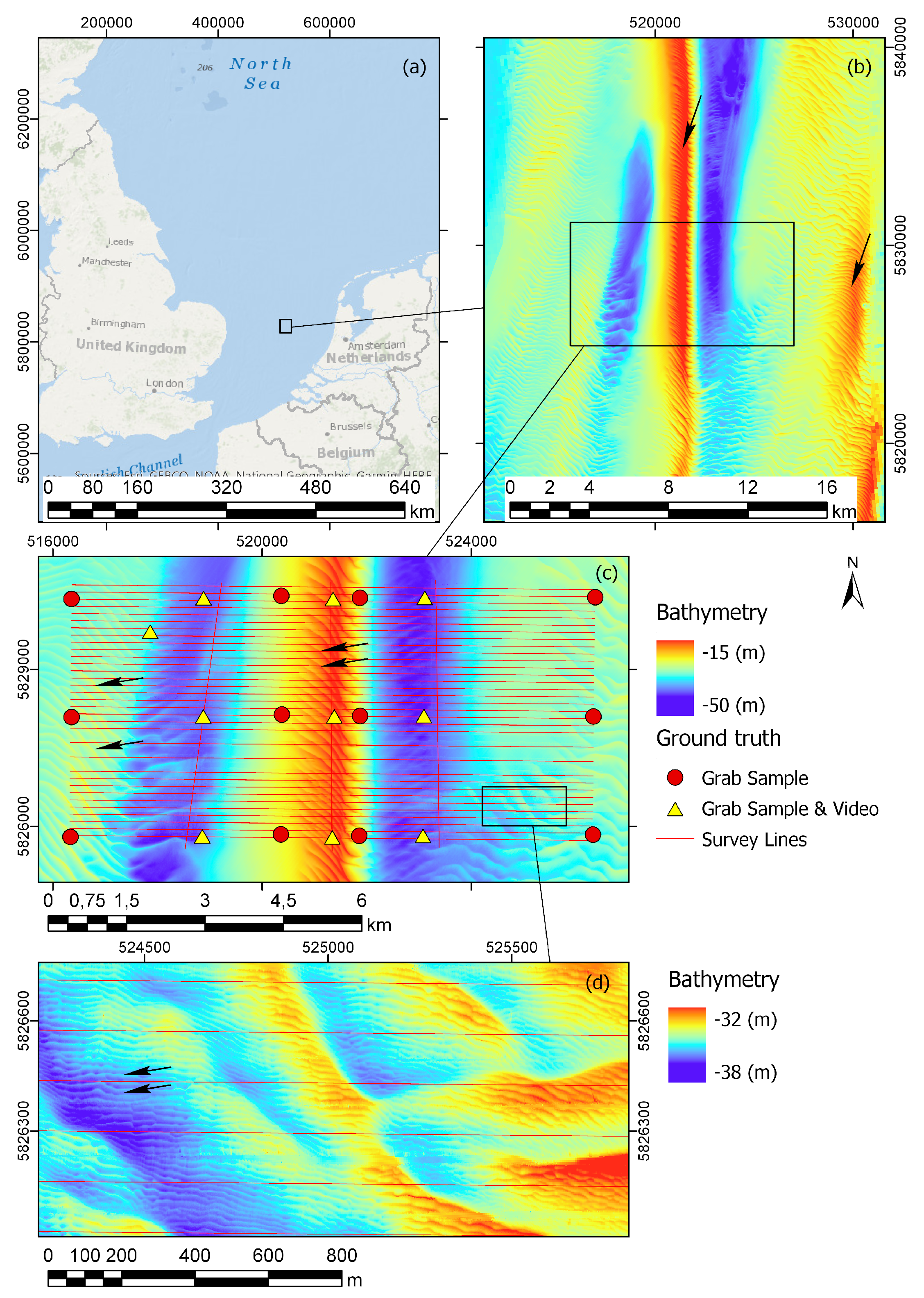
2.1. Study Area

The Brown Bank is located 85 km off the coast of the Netherlands, in the middle between the UK and the Netherlands, due west of Egmond aan Zee (52 32 59.994 N, 3 18 36.400 E; Figure 1). This area was visited in 2017 with the Royal Netherlands Institute for Sea Research (NIOZ) vessel, the Pelagia, from 27 October to 3 November (Cruise number/name: 64PE428disclose). Tidal currents in this area oscillate between a north eastern and south western flow direction with current flow rates exceeding 1 km/h. The average water current is in the north eastern direction [18]. The annual mean significant wave height is 2 m [19]. The main seabed substrate in this part of the North Sea is sand, with sand waves of various sizes clearly visible in the bathymetry. The dominant bathymetric features of the research area are sand banks (Figure 1b), which can be tens of meters high and have a length of 5–10 km [20]. In the study area there is mainly one sand bank, i.e., the most dominant one in the North Sea [20], which is called the Brown Bank. The Brown Bank runs from north to south, with a water depth on the top of the bank of ∼19 m, and a water depth in the troughs on either side being ∼45 m.
In addition to the sand banks, there are two other periodic bed forms that are defined in this paper as sand waves (Figure 1c) and megaripples (Figure 1d) [21], respectively. Sand waves occur with a wavelength of around 200 m, with the occasional wavelength as short as 100 m and others as long as 300 m. In [22] it was found that sand waves migrate at a rate of several meters per year, and that the migration speed is strongly correlated with the sand wave shape. Superimposed on the sand waves are megaripples [21], which have a wavelength of 15 m, where some wavelengths are as short as 10 m and others as long as 25 m. The megaripples move faster than the sand waves, in the scale of weeks [21,23] or even hours [24]. The troughs of the Brown Bank consist of muddy sediments mixed with gravel and shell fragments and the crests contain well sorted medium sand [17].

2.2. Multibeam Echosounder Data

2.2.1. Multibeam Echosounder Settings

The acoustic survey was performed with a hull-mounted Kongsberg EM 302 multibeam echosounder (MBES). The EM 302 has a central frequency of 30 kHz and has 2 and 1 beam opening angles in the across and along track directions respectively. Four transmit sectors were used during the survey, each using a slightly different frequency of 26.5 kHz, 30.5 kHz, 33.5 kHz, and 28.5 kHz for sectors 1 to 4. The beam coverage of the 432 beams was set to equidistant (vs. equiangular). A swath opening angle of 130 was used, with port and starboard coverage both being 65 . The pulse length was 750 μ s for the entire survey. The EM 302 has a sensitivity resolution of 0.1 dB. Bathymetry, backscatter, and water column data were recorded using Kongsberg’s native seafloor information system (SIS) software. A Seapath global positioning system (GPS) and motion reference unit (MRU) provided position and motion correction information. GPS information was fed into the MBES processing, therefore eliminating the need to perform tide corrections. The MBES data were corrected for roll, heave, and yaw.
The data from the Pelagia were cleaned using the following steps. Firstly, the data was imported into the QPS Qimera software, and a spline filter was used to flag data points that were depth outliers. Subsequently, the cleaned data from Qimera were imported into Qinsy to convert them into an ASCII tabular format. Further processing was then carried out in Matlab. Aeration artifacts were filtered out if the average backscatter over 15 adjacent pings was more than 1.5 dB lower than the average backscatter over the nearest 700 pings

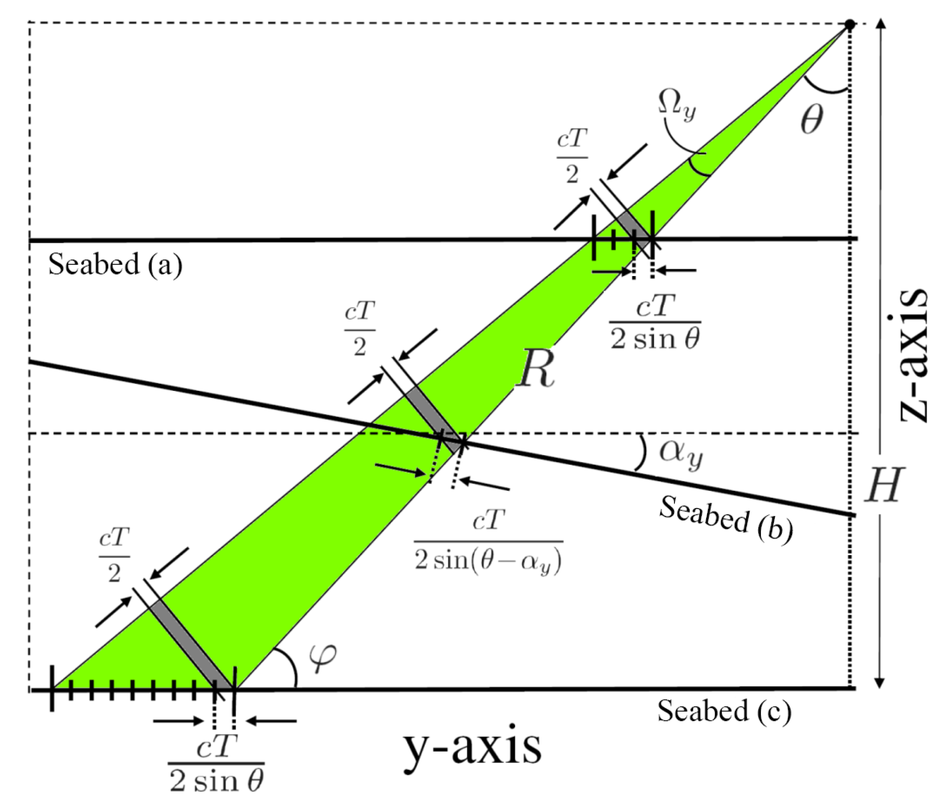
2.2.2. Backscatter Corrections for Seafloor Slopes

Because the survey area is dominated by sand waves and megaripples, with seafloor slopes as steep as 20 degrees, a slope-corrected grazing angle is needed. If not corrected, the significant slopes of the seafloor can in principle degrade the classification results. This is thus an essential pre-processing step because the Bayesian classification method uses the backscatter data at a specific grazing angle. We closely follow the pre-processing steps proposed by [15]. Figure 2 shows the across-track cross section of the signal footprint for three different environments, i.e., a shallow water, a deep water and a non-flat seafloor.
A three-step algorithm is employed to estimate and hence apply the corrections required due to the local slopes. The steps are as follows: (1) Estimating the along- and across-track seafloor slopes; (2) Correction of the true beam grazing angle; and (3) Correcting the backscatter data. These steps require the along- and across-track slopes in the time-varying coordinate system of the vessel. The details of the above steps are as follows.
Step 1 Estimation of local slopes
The least-squares method is employed to estimate the local slopes using the bathymetry data. The slopes are computed in the time-varying coordinate system of the vessel. The bathymetry data of a given MBES line was gridded to a grid size of 2 m × 2 m. Such a regular surface patch includes a few pings and beams around the central beam angle. For the discrete points within the surface patch, we then have z i = f ( x i , y i ) , i = 1 , , n , n indicating the number of bathymetry data within the surface patch. Here x i and y i refer to the along and across-track coordinates in relation to the vessel for point i. The surface patch is assumed to be a plane, with the form
f ( x , y ) = a 0 + a x x + a y y
consisting of three unknown coefficients a 0 , a x and a y . The model of observation equations is of the form z = A a , where z = [ z 1 , , z n ] is the n-vector of observations containing the bathymetry data within the 2 m × 2 m surface patch, a = [ a 0 a x a y ] is the vector of unknown parameters, and A is the n × 3 design matrix for which its i t h row is A i = [ 1 x i y i ] . Assuming the observations are independent and have identical variances, the least squares estimate of the parameters is a ^ = ( A A ) 1 . A procedure called ‘data snooping’ can also be used to test for the presence of outliers in the bathymetry data [25,26]. This will then leave out some outlying depth measurements when computing the local slopes.
Having estimated the parameters of the above surface patch f ( x , y ) , one can obtain the local slopes f x ( x , y ) = a x and f y ( x , y ) = a y where a x and a y are the ratios of the vertical to horizontal changes in the along and across-track directions respectively. Figure 3 shows one typical area in which the along and across-track slopes have been estimated. The signature of the megaripples is clearly visible from the computed slopes.
Step 2 Grazing angle correction
After estimating the local surface, the local slopes a x and a y of the plane are known (Equation (1)). The normal vector to the plane is the gradient of the surface, expressed as n = [ a x a y 1 ] . The nominal receiving-beam direction based on the flat surface in the z-y plane is provided as m = [ 0 sin θ cos θ ] , where θ is the nominal incident angle. The angle between the two vectors n and m is the true incident angle, given as
cos θ t = sin φ + a y cos φ 1 + a x 2 + a y 2
where φ = π 2 θ is the nominal grazing angle. Therefore, the nominal incident angle θ should be corrected to the true incident angle θ t . This is an essential step because the classification method uses the backscatter data at a specific angle.
Step 3 Backscatter correction
The local slopes also affect the backscatter data. This is because the received backscatter refers to a flat signal footprint A f [15]. In the presence of local slopes, the signal footprint will change and hence the corresponding backscatter values need to be corrected for the actual ensonified area A f using the along and across-track slope angles α x = arctan a x and α y = arctan a y [15] (Figure 2). The correction C of the backscatter for the actual ensonified area, expressed in decibels (dB) is given as
C = 10 log sin ( θ α y ) cos α x sin θ .
The corrected data is then supplied to the Bayesian classification method.

2.2.3. Bayesian Classification Method

This section provides an overview of the essential steps to generate the acoustic classification maps from the backscatter (BS) data. The central limit theorem expresses that the BS follows a Gaussian distribution for one sediment type, if sufficient independent measurements are considered for determining the BS values. For a given frequency and angle, the backscatter strength depends on the seabed properties. If the survey area contains m sediment types, the BS histogram of the backscatter data for a specific incident angle is then represented by a linear combination of m Gaussian distributions as
f ( y j | x ) = k = 1 m c k exp ( y j y ¯ k ) 2 2 σ y k 2
where y j is the BS value at bin ( y j , y j + Δ ) of the BS histogram, with j = 1 , , M and M being the total number of bins. The bin size Δ is set by the sensitivity resolution of the MBES. The vector x contains the unknown parameters of the Gaussian distribution: x = ( y ¯ 1 , , y ¯ m , σ y 1 , , σ y m , c 1 , , c m ) , where the triple ( y ¯ k , σ y k , and c k ) indicates the mean, standard deviation and contribution of each Gaussian distribution for k = 1 , , m . The curve fitting procedure is performed in an iterative manner for increasing m. The error in the fitting is tested by the χ 2 goodness of fit test, which is of the form
χ 2 = j = 1 M n j f ( y j | x ) 2 σ j 2
where n j denotes the number of backscatter measurements per bin j in the BS histogram. For n j a Poisson-distribution is postulated, indicating that the variance σ j 2 is equal to n j . The goodness of fit statistic has a chi-squared distribution with ν = M 3 m degrees of freedom. The goodness-of-fit criterion is then defined as the reduced chi-squared statistic, given by
χ ν 2 = χ 2 ν
which has a value close to 1 for a good fit, indicating that the difference between modelled and measured histograms fall within the uncertainties of the BS data. The value of m for which no significant improvement on the reduced chi-squared statistic is obtained, or when it has a value close to 1, can be considered to be the optimal value of m based on the backscatter data.
The final classification step uses the Bayes decision rule. The above m Gaussians introduce m hypotheses as H k , k = 1 , , m which correspond to the m seafloor sediment types. It is assumed that the hypotheses are equally likely and the Bayesian decision rule for multiple hypotheses then indicates to accept H k if max i f ( y j | H i ) = f ( y j | H k ) . Given the observation y, the hypothesis that maximizes the likelihood f ( y | H ) gets accepted. Thus, in principle, the intersections of the m Gaussians result in m non-overlapping acceptance regions A k , corresponding to m acoustic classes (ACs).

2.2.4. Two Levels of Data Averaging

To ensure that the central limit theorem is satisfied, namely the backscatter strength per angle and sediment type is Gaussian distributed, the backscatter values used should be the result of a sufficient number of independent measurements. The backscatter per beam is an average value, i.e., the result of N s measurements, with N s representing the number of signal footprints (or scatter pixels) within the beam footprint, see Figure 2. Sometimes the number of scatter pixels in a beam is small. Then the backscatter values are averaged over a certain number of neighboring beams and consecutive pings. This, though reducing the spatial resolution, ensures that each BS value is representative of a sufficient number of scatter pixels. In addition, a larger number of scatter pixels per backscatter strength value provides narrower Gaussian distributions per sediment type, i.e., increased geo-acoustic resolution. For beams away from nadir, the ensonified area A f is (much) smaller than the beam footprint. Therefore many scatter pixels fall within the footprint of the receiving beam. The number of scatter pixels N s within a beam is a function of θ and α y , and is given by
N s ( θ , α y ) = R Ω y cos ( θ α y ) c T 2 sin ( θ α y )
where Ω y is the beam aperture in the across-track direction, c is the average water sound speed, T the length of the transmitted pulse, and R = H / cos θ , where H is the water depth. Equation (7) only holds for the beams sufficiently away from nadir. For beams closer to nadir the ensonified area is limited by the beam aperture and not the projected pulse duration. Thus, the nadir beams have only one scatter pixel.
To investigate the trade-off between the spatial and geo-acoustic resolution, two levels of data averaging were performed. In the first averaging scheme, no averaging was done as long as a data point was based on 20 or more scatter pixels, which was the case for the outer beams. If a data point had less than 20 scatter pixels, it was averaged with the geographically nearest neighbors until it was representative of at least 20 scatter pixels.
For the second scheme the data of a given MBES line was gridded to a grid size of 2 m × 2 m. The average backscatter and the average depth of all the points in a grid cell are used to form a single data point for that grid cell. It was further required that a grid cell contained at least 10 data points, otherwise the data within that grid cell was discarded. The advantage of this method is that the averaging of the backscatter increases, and hence it reduces noise in the classification results. The disadvantage is that it decreases the number of data points used in the classification, and thereby decreases the spatial resolution of the classification.

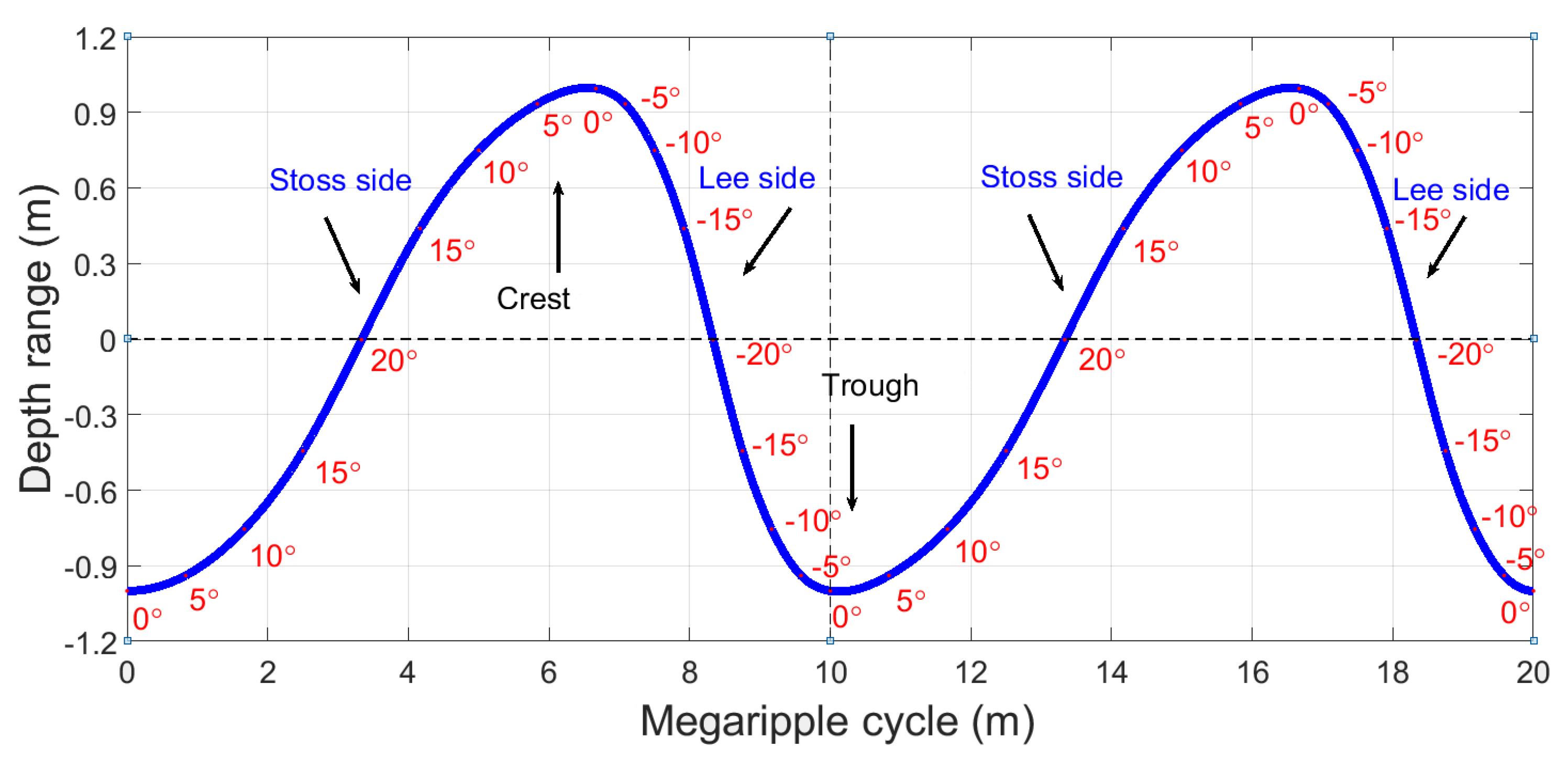
2.2.5. Megaripple Partitioning

To investigate the distribution of sediments over megaripples, thirty two areas with a size of ∼100 m × 100 m, where a clear megaripple pattern was present, were selected for further study. Using the orientation of the megaripples and the values of the absolute slopes, a direction specific slope was computed such that positive slopes would be on the stoss side (the side that receives dominant tidal current, also the less steep side) and the negative slopes would be on the lee side of the megaripple (Figure 4). The polarity of the computed slopes thus separated the area into the different sides of a megaripple. Further subareas were created by defining the crests and troughs of the megaripples. This was done by fitting a plane Z = f ( E , N ) = a 0 + a 1 E + a 2 N to the bathymetric data using the least squares method. Here E and N refer to the easting and northing coordinates of the bathymetry data in a UTM (Universal Transverse Mercator) coordinate system. The points above the fitted plane are classified to be on the crest, and those below the plane, in the trough of the megaripple. The area was then binned based on the directional slope, ranging from −20 to 20 degrees with a bin size of 5 degrees (Figure 4). The bin centers are then at −17.5, −12.5,…, 17.5 degrees. The mean and mode occurrences of acoustic classes was calculated per bin and per trough and crest area for each of the 32 selected areas and used for determining sediment patterns over megaripples.

2.3. Video Data

Videos of the seabed were collected along 150 m transects at 10 stations (Figure 1c) with a towed video camera system. This system was inspired by the one used in [27]. The aluminum frame houses a remote controlled forward-facing video camera (Kongsberg OE14-522A-0009 Colour HD Pan), a downward facing DSRL camera (NIKON D750), eight lights (Fisheye FIX NEO 1000DX SW II LED), and two sets of lasers (Z-Bolt, SCUBA-II green) with a fixed separation distance. The video camera was set to view the seabed just in front of the frame. Moreover, the frame was equipped with multiple floats, resulting in a small positive buoyancy. Two drag chains underneath the frame cause for negative buoyancy. The varying length of the part of the drag chain which touches the seabed stabilizes the frame’s height above the seabed. Three towing cables were attached to the frame at different points, which were combined after 6.5 m into one towing cable. A drop weight of 55 kg was attached to this merging point, which reduced the vertically oriented towing forces of the vessel on the frame. The video camera was connected to a computer on-board with a video data “umbilical cord”, which was held in place separate from the towing cable. Using the live stream from the video camera, the length of the towing cable was adjusted to maintain seabed view during transects. During video operations, the vessel had a speed of ∼0.1 m/s.
The collected video footage was analyzed and the superficial seabed type determined. The time of every observed change in seabed type was recorded. All recordings in which the seabed was not (clearly) visible, due to particle clouds or motion, or in which at least one of the lasers was not visible were defined as invalid. The position of the camera was estimated based on a time-match with the position of the vessel, which was saved by the vessel’s logging system every 30 s. As the distance between the camera and vessel varies, depending on the prevailing depth and current, the exact position of the camera cannot be determined. However, because the camera was deployed on the starboard side of the vessel, with as little towing cable as possible, we assume the positioning error to be >10 m but <100 m.

2.4. Grab Sample Data

Twenty two grab sample locations were selected, with twenty one of these falling on a regular grid. That includes seven vertically oriented parallel lines each with three locations; in the eastern most border of the survey area, in the troughs on both sides, on the slopes on either side, and on the crest of the Brown Bank, and in the western most border of the survey area (Figure 1). At each sampling location three replicate samples were taken resulting in a total of 66 grab samples. The grab samples were acquired with a 30 cm Box Core. Subsamples were taken for particle size analysis (PSA). Between the time that the samples were gathered until they were processed in the lab, they were stored at −20 C. Prior to PSA the samples were freeze-dried. For the particle size analysis the contents of the sample were successively sieved over 4, 2, and 1 mm sieves and the weights of these fractions were measured. The particles that were larger than 2 mm were separated to determine the gravel fraction. The grain size distribution of the portion smaller than 1 mm was determined by means of laser diffraction with a Malvern Mastersizer 2000 (Malvern Instruments, Worcestershire, UK). The sieving and laser diffraction results were combined by scaling the results from the Malvern by the mass proportion of the sample that was smaller than 1 mm. This combined dataset was then used for further analysis.
The results of the grab sample sieving process were converted into the phi grain size units by using ϕ = log 2 d , where d is the representative diameter of the grains in millimeters. Two measures are often used to describe the sediment grain size of a grab sample, that is, the median or the mean grain size. The median corresponds to the 50th percentile on the cumulative curve of which half the particles by weight are larger and half are smaller than the median. It is therefore of the form M z = ϕ 50 . The mean is the average grain-size for which several formulas are used in the literature. The most commonly used formula is that given by [28]
M z = ϕ 16 + ϕ 50 + ϕ 84 3
where ϕ 16 , ϕ 50 and ϕ 84 represent the size at the 16th, 50th, and 84th percentiles of the sample by weight. For the work presented here the mean grain size is used; but similar results are obtained using the median grain size.
In addition to the mean grain size, provided by Equation (8), statistics for sorting σ (Equation (9)), skewness s (Equation (10)), and kurtosis k (Equation (11)) of the grain size distribution were also calculated [28].
σ = ϕ 84 ϕ 16 4 + ϕ 95 ϕ 5 6.6
s = ϕ 16 + ϕ 84 2 ϕ 50 2 ( ϕ 84 ϕ 16 ) + ϕ 5 + ϕ 95 2 ϕ 50 2 ( ϕ 95 ϕ 5 )
k = ϕ 95 ϕ 5 2.44 ( ϕ 75 ϕ 25 )
These were used to create a feature matrix Y = [ M z σ s k ] . Principal component analysis of this matrix, which is of size 66 × 4 , was performed and the most informative principal components (PCs) were selected. These are then used to determine the correlation between the acoustic classification results and the full grain size spectrum of the grab samples.
Folk classification of the grab samples is also used. According to this classification method, sediments are given a descriptive label based on the proportions of Mud, Sand, and Gravel. Gravel particles are those larger than 2 mm, Sand those between 2 mm and 0.0625 mm, and Mud what is less than 0.0625 mm. A 0.01% boundary was used between a “no gravel” content and a “slightly gravelly” label.

3. Results and Discussion

3.1. Acoustic Classification Results

The classification method of Section 2.2.3 is now applied to the backscatter (BS) data that was cleaned and pre-processed according to the description in Section 2.2.2. That is, the correct grazing angles are known and the backscatter data has been corrected for the change in the ensonified area induced by the seafloor slopes.
In the first step, the number of sea bottom types, distinguishable in the acoustic data, is determined. This is achieved by increasing the number of Gaussians to well describe the histogram of the BS values at a given grazing angle. The number of seafloor types, m, was found to be 4 (Figure 5). The beam angles used to create the histograms and to perform the Gaussian fitting procedure were the 30 , 28 , and 26 grazing angles, for both the port and starboard sides. The error bars in Figure 5 give the standard deviation of the χ ν 2 statistic, 2 / ν . Because the backscatter data from the EM 302 multibeam is recorded at a resolution of 0.1 dB the number of bins M per histogram tended to be well above 100. The variable ν gets larger with larger M and therefore the standard deviations of the χ ν 2 statistic, represented by the error bars in Figure 5, become small.
Figure 6 shows the BS histograms along with their best fit for the grazing angles 30 , 28 , and 26 . The intersecting points of the corresponding probability density functions (PDFs) are used to form the acceptance regions of the four classes. The percentages of the histogram at these reference angles that fall into a specific class were then recorded and used to divide, and thereby classify, the histograms for the grazing angles from 65 to 25 .
The acoustic classification results are presented in Figure 7. The broad scale classification results fall into the following patterns. For water depths shallower than 25 m, on the crest of the Brown Bank, mainly acoustic classes 1 and 2 occur. Lower classes (1 and 2) generally correlate with smaller grain sizes [12]. In the troughs on either side of the Brown Bank, for water depths deeper than 35 m, the classes are higher, mainly classes 3 and 4. In the remainder of the area the classes tend to be a mixture of classes 2 and 3.

3.2. Ground Truth Data

In total there were 16,594 classified, and geo-referenced, seconds of valid video footage (video frames, Table 1). In all areas where video data was collected “Sand with a ripple structure” was found (Figure 8). The presence of shell fragments (Figure 8b), smaller and larger stones (or Granules and Pebbles according to the Udden-Wentworth grain size classification scheme [29]) (Figure 8c), and Sabellaria fragments (Figure 8d) varied from one area to the next. Figure 9 represents the video classification results overlaid on the acoustic classes. The class “Sand with hardly any shell fragments” was only found on the crest of the Brown Bank, see Figure 9 (upper right). The remaining 3 classes were all found in the troughs on either side of the Brown Bank.
At Station 2 (Figure 9, upper left), alternating video classes of “sand with some shell fragments” and “sand with small stones and incidental larger stones” are seen. The alternation matches with the wavelength of the megaripples in this area. The acoustic classification also alternates on this spatial scale, between class 4, as the highest class, and class 3 or 2 for the lower classes. The video data at Station 8, containing “Sand with hardly any shell fragments”, have mainly lower acoustic classes 1 and 2. At Stations 9 and 14 (lower parts of Figure 9) the video is classified as mostly “Sand with some shell fragments”. However, some frames are classified as also having either “Small stones and incidental larger stones” at Station 14, or “Sabellaria fragments and incidental larger stones” at Station 9. Their locations match with areas of higher acoustic classes (Figure 9).
To further investigate the relation between the video data and the acoustic classification results, the two datasets were geographically matched, and the occurrences of the acoustic and video classifications were counted. The mode of the acoustic class within a one-meter radius was used. If there were no acoustic classes within this radius then the video data point was discarded. The results are presented in Figure 10. In areas where the video recordings indicate “sand with no shell fragments” the occurrence of acoustic class 1 is dominant. There are no instances of acoustic class 4 in these areas. In areas where the video data indicate the presence of “sand with some shell fragments” the occurrence of acoustic classes 2 and 3 is highest at 32% and 49%. For “Sand with Sabellaria fragments and incidental larger stones” and “Sand with small stones and incidental larger stones” the distribution of acoustic class occurrences is very similar, with higher percentages for the higher acoustic classes. There were hardly instances of acoustic class 1 in these areas.
As for the grab samples, the majority have a mean grain size ranging from M z = 1.50 ϕ to M z = 1.75 ϕ . The standard deviation of the mean grain sizes from the three samples taken at each station was at the same level as the size range of all the samples i.e., σ M z = 0.25 ϕ . There was one triple of grab samples (from Station 23) with a smaller mean grain size, M z = 4.04 ± 1.18 , than the rest of the grab samples. The grab at this station was composed of very fine particles that were compacted and stuck together. For most grab samples, clumps of particles that were stuck together could be brushed lightly in order for them to be sieved. The grab samples from Station 23, however, had to be crushed through the various sieve sizes with force. After doing this, the particle size analysis (PSA) indicated small grain sizes for this grab sample.
Often, backscatter-based acoustic classes are compared to the mean grain sizes to create sediment maps [11,30,31]. Figure 11a shows the results of such a comparison. It can be seen that the acoustic classification results are not correlated with mean grain size values. This observation not only holds when the mean grain size is compared with the acoustic classes, but also when the mean grain size of a grab sample is compared to its Folk classification (Figure 11b). Thus, a grab sample with different Folk class can have the same mean grain size.
When using Folk classes, the sediments “sandy mud” (sM), “sand” (S), “slightly gravelly sand” ((g)S), and “gravelly sand” (gS) were encountered. Out of the 22 grab sample positions there is 1 location that is classified as sM. There were 5, 15, and 1 locations that were classified as S, (g)S and gS, respectively. Thus, the dominant sediment types in the surveyed area is either sand or slightly gravelly sand again indicating an almost non-distinctive sedimentary environment.
The number of matches between the Folk class and acoustic class at the grab sample locations shows a general trend of coarser sediments for higher acoustic classes (Figure 12). Sand corresponds mainly to acoustic classes 1 and 2. Slightly gravelly sand is matched dominantly with acoustic classes 2 and 3, and gravelly sand with acoustic class 3. However, the finest sediment sM correlates with acoustic class 4. This is likely due to the compactness of the sediment for this grab sample, as was described earlier. We may assume that (g)S of the grab samples corresponds to “Sand with some shell fragments” in the video data. This correspondence is also observed when comparing the grab samples and acoustic classes in Figure 12 with the video data and acoustic classes in Figure 10.

3.3. Full Spectrum of Grain Size Distribution for Classification

Based on the mean grain size of the grab samples, the survey area is very homogeneous. However, both the Folk classes of grab samples and the acoustic data indicate four sediment types. This indicates that the acoustic classes are to be attributed to the full spectrum of the grain size distribution and not just the mean grain size.
This hypothesis is now investigated by using the variables M z , σ , s , and k from Equations (8)–(11) and performing PCA on these as explained in Section 2.4. The first PC, representing 53% of the feature variabilities, is not far from being just the sign-corrected average of the above four features with the dominant contributions from σ , M z and s. This PC is thus considered to be the most informative feature and hence will be used for comparison. Figure 13 shows this PC versus the acoustic classification results. A positive correlation is observed. This verifies that the full spectrum of the grain size distribution should be used when comparing grab samples with the acoustic classes and not just the mean grain size.
From the literature, it is expected that higher backscatter values would correspond to larger grain sizes. As indicated in Figure 11 there is no correlation with higher acoustic classes (which correspond to higher backscatter values) for larger mean grain sizes, because the mean grain size does not vary much over the grab samples. To check what influence larger grains have on backscatter values, the backscatter values from the beam angles ranging from 25 to 65 degrees were averaged over a few pings around each grab sample. These averaged backscatter values were compared to the percentage of the grab sample with a grain size greater than 0.5 mm (Figure 14). This showed that larger percentages of large grain sediments correspond to higher backscatter values (the linear correlation coefficient is 0.51). This finding is in agreement with the results presented by [32] who found a positive correlation between backscatter levels and shell or gravel percentage of grab samples. It can therefore be concluded that the areas of high backscatter values (classes 3 and 4) correspond to slightly gravelly sand and lower backscatter values (classes 1 and 2) correspond to sand. Further investigation would be needed to quantify the influence of other factors affecting backscatter strength, such as surface roughness and volume scattering [33].

3.4. Geo-Acoustic Versus Spatial Resolution

The classification of sediments in the Brown Bank area brings to the forefront a dilemma of resolutions. On the one hand sediments may vary from crest to trough of some of the smallest sand waves, i.e., megaripples, which have a wavelength of a few tens of meters. It would be desirable to accurately classify sediments over these features at a high spatial resolution. On the other hand a high geo-acoustic resolution is needed to account for small changes in sediment composition from the crest to the trough of the megaripple. When applying the Bayesian classification method, the geo-acoustic resolution is increased when the data points are representative of a higher number of scatter pixels due to the standard deviation of the Gaussians being less. The theoretical standard deviation of the Gaussians is σ y = 5.57 / N s , where N s is the number of scatter pixels [13]. An approach to increasing the number of scatter pixels per data point is to average the backscatter (BS) data over several beams in the across track direction, and several pings in the along track direction as employed by [15]. Performing such an averaging procedure has the added benefit of averaging out much of the ping to ping variability of backscatter data that is not dependent on the seafloor properties. While such averaging increases the geo-acoustic resolution, it directly decreases the spatial resolution of the classification.
For determining a good trade-off, the acoustic data were preprocessed with different levels of averaging (see Section 2.2.4). Figure 15 shows the fits of a Gaussian PDF to the BS histogram at the 26 starboard grazing angle for both approaches. A few observations are highlighted:
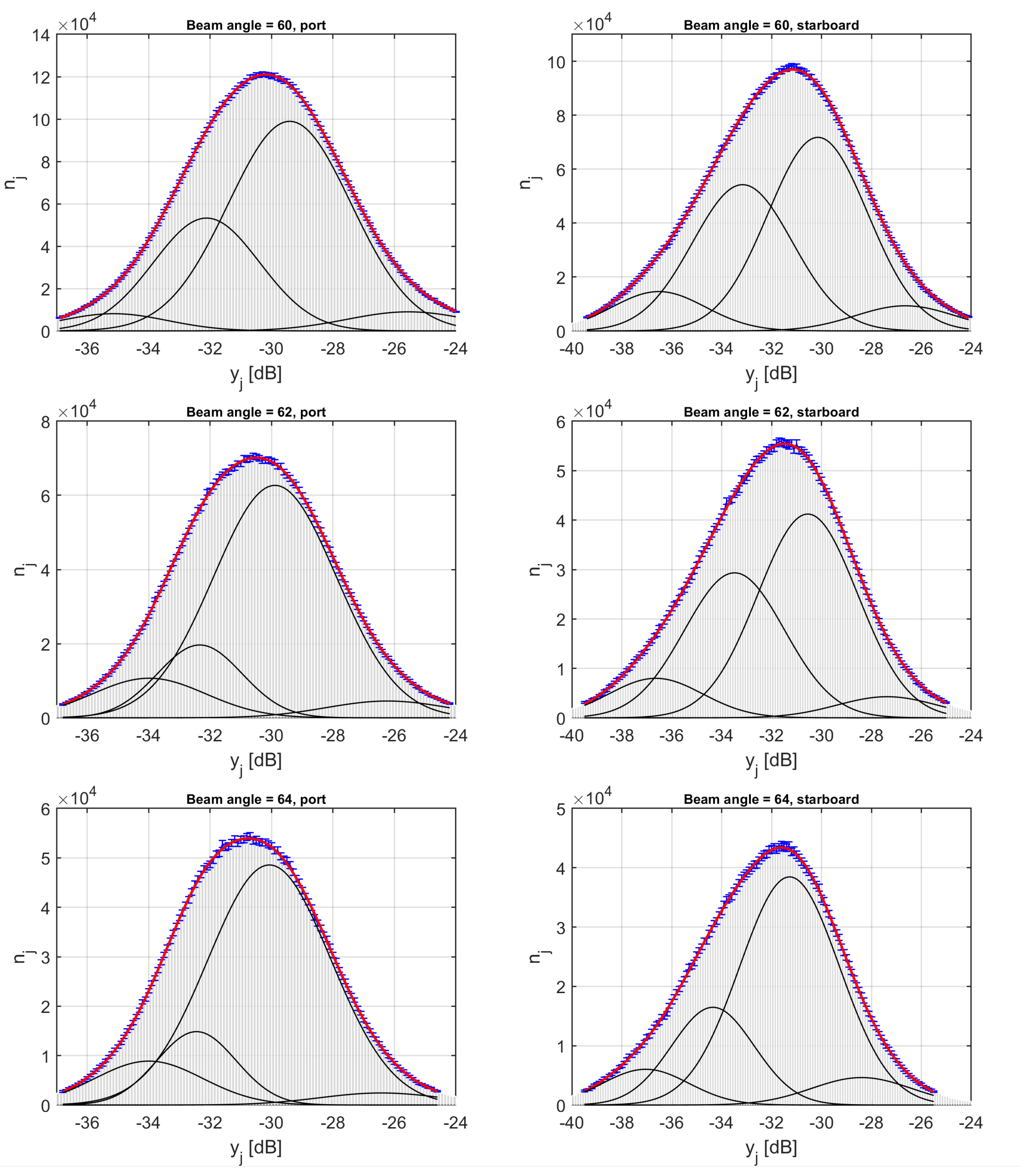
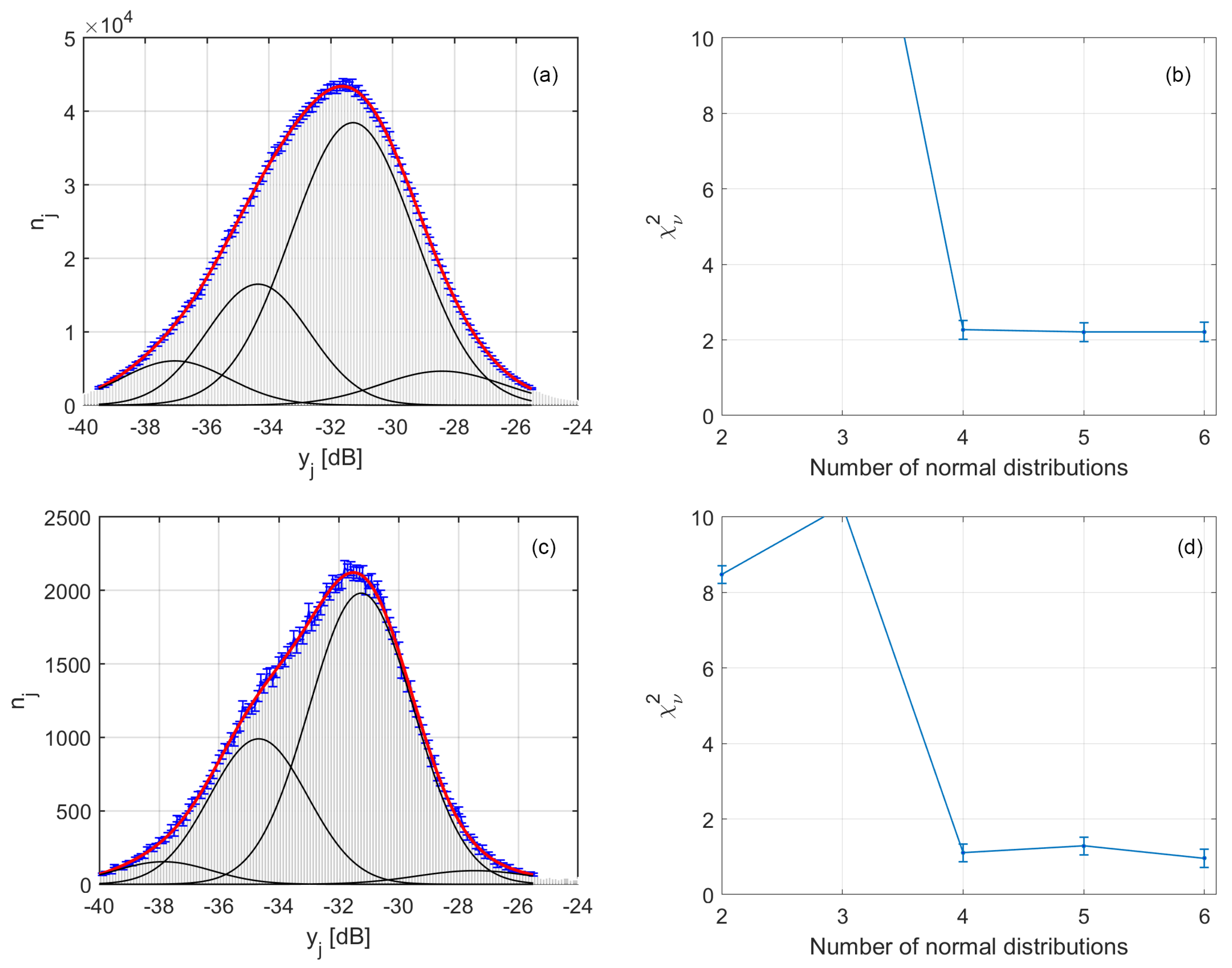
  • The above averaging procedure can in principle reduce the noise of the backscatter data. This may, however, not decrease the standard deviation proportionally to the square root of the number of scatter pixels represented. This is because this rule is valid only for independent and identically distributed data. This cannot be the case for the backscatter data averaged over a small surface patch, because the variation and uncertainty in the BS data has independent and dependent components. The independent component is known as noise, which can be averaged out. This however does not hold for the dependent component, which is intrinsic to acoustic sediment properties and its heterogeneity. The fact that the two histograms in Figure 15 look similar also verifies the above reasoning; otherwise the second data set would have a significantly narrower histogram due to the averaging procedure.
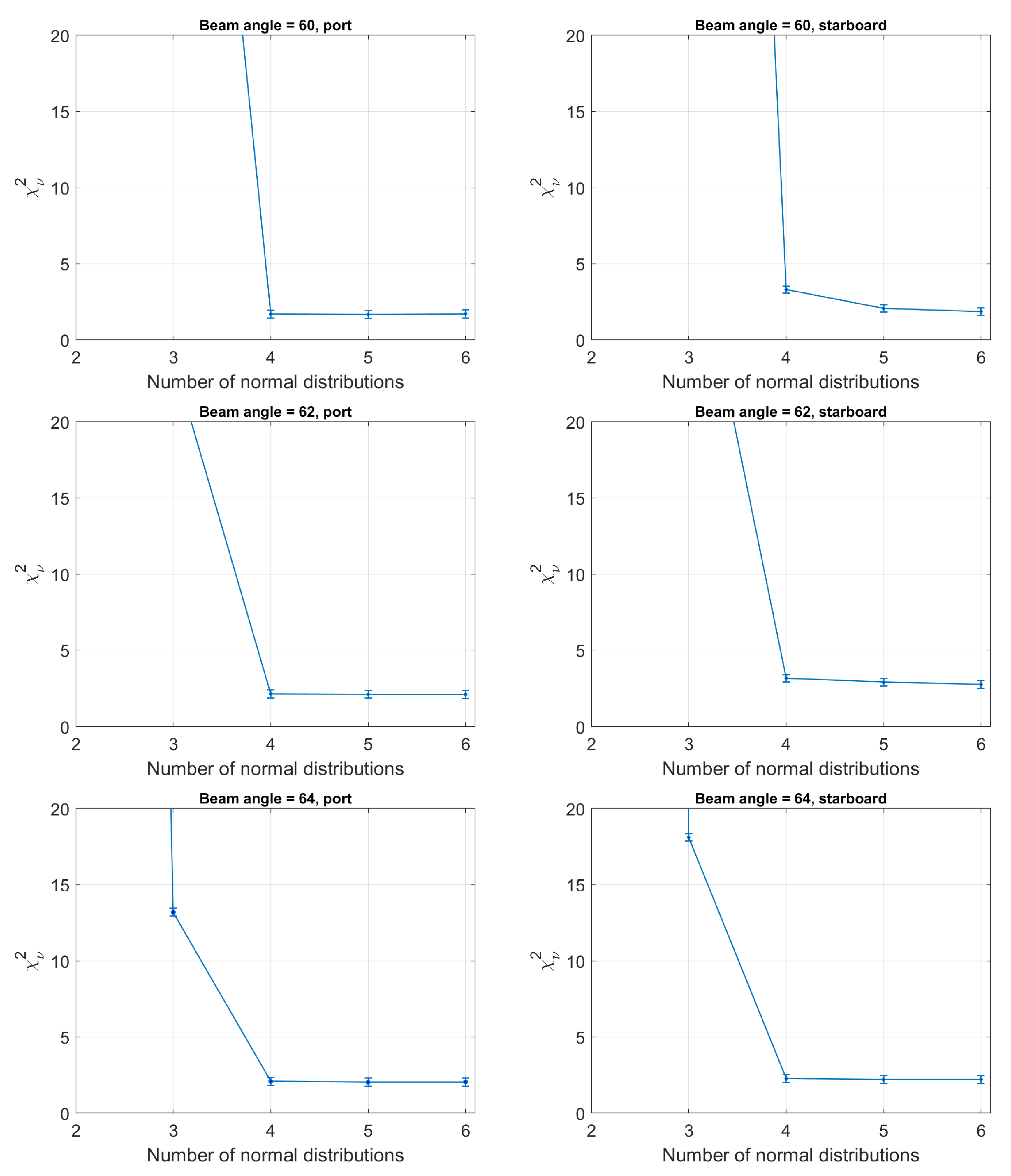
  • There is a trade-off between the spatial and geo-acoustic resolutions. While heavier averaging increases the geo-acoustic resolution of the classification, it directly decreases its spatial resolution. Narrower and relatively more separated Gaussians as well as chi-squared values closer to 1, obtained for the averaged data set (Figure 15 bottom subplots), indicate a better geo-acoustic resolution.
  • The results obtained in Figure 15 show that the means and standard deviations of the Gaussians are characteristic of the acoustic properties of the sediment types. Given that the mean grain sizes of the grab samples suggested a homogeneous seabed in this survey area, it might be thought that if the parameters of the Gaussian were given a significant range within which they could vary, only one (or a few) Gaussians would be fitted to the entire histogram. The results show that this is not the case. For both datasets, the bounds for the standard deviation were set to a range of 0.5–2 dB but for neither dataset were the lower or upper bounds used after the curve fitting was implemented. This indicates that the Bayesian classification results are not significantly affected by the averaging procedure.

3.5. Classifying Sediments Over Megaripples

Now we investigate to what extent MBES backscatter data can be used to classify the sediments over megaripples. This is of particular interest for detailed habitat mapping [34], engineering projects such as offshore wind farms or pipe laying [22], and for modelers of sand waves who study the morphology, hydrodynamics, and sand transport at the seafloor [1,24]. In the previous sections it is found that higher acoustic classes correspond to sediments with a larger proportion of coarse sediments in this study area. These terms will thus be used interchangeably in the following paragraphs.
Thirty two areas where megaripples were present were selected and partitioned as described in Section 2.2.5; see Figure 16 for two examples. Figure 17 shows the histogram of the maximum slopes computed for the above-mentioned areas. For these areas the occurrences of acoustic classes per location on the megaripples were counted. These classification results for the slope bin centers are presented in Figure 18. At the lowest point of the stoss side of the trough, i.e., bin center (BC) = 2.5 , the dominant AC is 3 (Figure 18, right). From the trough moving towards the crest, this gradually changes from higher classes to lower classes. The finest sediments (class 1) are found on the stoss side at BC = 17.5 , for both the trough and crest areas. Continuing towards the crest, the sediments are classified as either class 2 or class 3. At the highest point on the lee side of the crest, BC = 2.5 , the dominant acoustic class is again 3. This tends to become coarser when continuing down the crest towards the trough on the lee side. At BC = 17.5 , the steepest point on the lee side, on the boundary between the crest and trough areas (specified by rectangles in Figure 18), a mixture of acoustic classes, ranging from fine to coarse (class 1 to 4), is observed. This is also clearly visible in the two typical areas (out of the 32) in Figure 19. An important characteristic of this part of the megaripples, is that the coarsest sediments appear only here (see also Figure 19, left). In the remaining parts of the trough, at BC = 12.5 , 7.5 , and 2.5 , the sediments are again classified as coarse-grained.
To create a generalized acoustic class per position on the megaripple structure a weighted average of the dominant acoustic class was calculated for each slope bin, side of the megaripple, and trough or crest area. This can be considered a combining of the classification results presented in Figure 18. The result is shown in Figure 20. The alternating green and red line on the steepest part of the lee side slope indicates that the entire range of acoustic classes was found on this part of the megaripple. We hypothesize that this is a result of megaripple migration.
Megaripples migrate towards the lee side, known based on bathymetry comparisons with older data. This is also the average flow direction. We hypothesize that fine suspended sediments are deposited on the lee side of the megaripple. Then low acoustic classes are expected. At times of high tidal currents, the combination of the steep slope and a downward current causes an avalanche of the fine sediment deposition [24], leaving only the coarse sediments exposed. For that area high acoustic classes are then expected. This is why such a range of acoustic classes are encountered on the steepest leeward slopes of the megaripples.

4. Summary and Conclusions

The Bayesian classification method was applied to MBES backscatter data gathered in the Brown Bank area of the North Sea. To obtain reliable classification results, steep and rapidly changing slopes over tens of meters had to be corrected for. Acoustic classification results were then compared with video and grab sample data.
Based on the results of the sediment grain size analysis it was found that the seafloor sediments of the Brown Bank area are very homogeneous. The variance in the mean grain size over the entire area was at the level of the variance within the triplicate grab samples from individual sampling stations. However, Folk classification of grab samples, as well as, the acoustic classification results were more discriminative. A further analysis showed that for areas like the Brown Bank, the full grain size distribution should be used when classifying the grab samples and when relating this ground truth data to the acoustic classification results. This should be taken into account for any future sediment studies in homogeneous sandy environments.
For acoustic classification of sediments in relatively homogeneous environments, especially over megaripple structures, high spatial and geoacoustic resolutions are required. There is, however, a trade off in these resolutions. Therefore, depending on the aim of a classification application, either of these resolutions can be optimized for. It was found that the Bayesian classification method remains statistically sound when optimizing for the spatial resolution, as long as the number of scatter pixels used in the averaging satisfies the central limit theorem requirements. This is a pivotal result that underscores the validity of our acoustic classification results over megaripples.
The results revealed that there was a significant sorting of sediments over megaripples. Higher acoustic classes, and therefore coarser sediments, were found in the troughs and on the crests. Low acoustic classes were consistently found to be on the steepest part of the stoss side of a megaripple. On the, even steeper, lee side slope of the megaripple a mixture of all acoustic classes was found. These detailed results have a number of implications. First, for detailed habitat maps, the size of the megaripple and not that of the sand wave should define the resolution scale of the map. Next, researchers gathering ground truth data, such as grab samples and video data, should strive to geo-reference the point measured on the seafloor with an accuracy well below the wavelength of megaripples to avoid ambiguities in measurement. Finally, it confirms that the classification of backscatter data from MBES systems is a powerful method to further study and display the spatial distribution of sediments over megaripple bed forms. As such, it can provide valuable information for habitat mapping, engineering projects such as offshore wind farms or pipe laying, or to serve as field validation data for sand wave modelers.

Author Contributions

Conceptualization, L.K., A.A.-S., M.S. and D.G.S.; Data curation, L.K. and K.J.v.d.R.; Formal analysis, L.K., A.A.-S., K.J.v.d.R., M.S. and D.G.S.; Funding acquisition, D.G.S. and M.S.; Investigation, L.K., A.A.-S., K.J.v.d.R. and S.O.; Methodology, L.K., A.A.-S., K.J.v.d.R., S.O., M.S. and D.G.S.; Project administration, L.K., A.A.-S., M.S. and D.G.S.; Resources, L.K., K.J.v.d.R. and S.O.; Software, L.K. and A.A.-S.; Supervision, M.S. and D.G.S.; Validation, L.K., A.A.-S., K.J.v.d.R., S.O. and M.S.; Visualization, L.K. and A.A.-S.; Writing—original draft, L.K., A.A.-S., K.J.v.d.R. and S.O.; Writing—review & editing, L.K., A.A.-S., K.J.v.d.R., M.S. and D.G.S.

Funding

This research is part of the multidisciplinary research project DISCLOSE. DISCLOSE is a joint venture of the Delft University of Technology, the University of Groningen, the Royal Netherlands Institute for Sea Research, as well as the North Sea Foundation. DISCLOSE is funded by the Gieskes Strijbis Fonds.

Acknowledgments

The authors would like to thank Rob Witbaard for being the chief scientist during the data gathering cruise and the crew of the NIOZ vessel the Pelagia for all of their assistance during the acquisition of the data. Karline Soetaert of NIOZ is acknowledged for her role in organizing the cruise, as well as Tom Ysebaert, who also coordinated the particle size analysis of the grab samples. Peter van Breugel was key in performing the particle size analysis in the NIOZ lab. Laura Govers and Han Olff of the University of Groningen are acknowledged for their valuable comments to earlier versions of this manuscript. We also thank Leendert Dorst and Daniëlle van Kuijk of the Hydrographic Service within the Royal Netherlands Navy for making full coverage bathymetry data of the Brown Bank area available. We acknowledge the Gieskes-Strijbis Fonds for the financial support of the DISCLOSE project, within which this research took place.

Conflicts of Interest

The authors declare no conflict of interest. The funders had no role in the design of the study; in the collection, analyses, or interpretation of data; in the writing of the manuscript, or in the decision to publish the results.

Abbreviations

The following abbreviations are used in this manuscript:
MBESMultibeam echosounder
SBESSinglebeam echosounder
BSBackscatter
NIOZRoyal Netherlands Institute for Sea Research
SISSeafloor information system
GPSGlobal positioning system
MRUMotion reference unit
UTMUniversal Transverse Mercator
PDFsProbability density functions
ACAcoustic class
PSAParticle size analysis
sMSandy mud
SSand
(g)SSlightly gravely sand
gSGravely sand
PCAPrincipal component analysis
PCPrincipal component
BCBin center
DISCLOSEDIstribution, StruCture and functioning of LOwresilience benthic communities
and habitats of the Dutch North SEa
dBDecibel
mMeter
mmMillimeter
μ mMicrometer
μ sMicrosecond

References

  1. Roos, P.C.; Wemmenhove, R.; Hulscher, S.J.; Hoeijmakers, H.W.; Kruyt, N. Modeling the effect of nonuniform sediment on the dynamics of offshore tidal sandbanks. J. Geophys. Res. Earth Surf. 2007, 112, 2005JF000376. [Google Scholar] [CrossRef]
  2. Stolk, A. Variation of sedimentary structures and grainsize over sandwaves. Mar. Sandwave Dyn. 2000, 1, 23–24. [Google Scholar]
  3. Svenson, C.; Ernstsen, V.B.; Winter, C.; Bartholomä, A.; Hebbeln, D. Tide-driven sediment variations on a large compound dune in the Jade tidal inlet channel, Southeastern North Sea. J. Coast. Res. 2009, 1, 361–365. [Google Scholar]
  4. Van Lancker, V.; Jacobs, P. The dynamical behaviour of shallow-marine dunes. In Proceedings of the International Workshop on Marine Sandwave, Lille, France, 23–24 March 2000; pp. 213–220. [Google Scholar]
  5. Brown, C.J.; Smith, S.J.; Lawton, P.; Anderson, J.T. Benthic habitat mapping: A review of progress towards improved understanding of the spatial ecology of the seafloor using acoustic techniques. Estuar. Coast. Shelf Sci. 2011, 92, 502–520. [Google Scholar] [CrossRef]
  6. Marsh, I.; Brown, C. Neural network classification of multibeam backscatter and bathymetry data from Stanton Bank (Area IV). Appl. Acoust. 2009, 70, 1269–1276. [Google Scholar] [CrossRef]
  7. Ojeda, G.Y.; Gayes, P.T.; Van Dolah, R.F.; Schwab, W.C. Spatially quantitative seafloor habitat mapping: Example from the northern South Carolina inner continental shelf. Estuar. Coast. Shelf Sci. 2004, 59, 399–416. [Google Scholar] [CrossRef]
  8. Clarke, J.H.; Danforth, B.; Valentine, P. Areal seabed classification using backscatter angular response at 95 kHz. In Proceedings of the SACLANTCEN Conference on High Frequency Acoustics in Shallow Water, Lerici, Italy, 30 June–4 July 1997; pp. 243–250. [Google Scholar]
  9. Lamarche, G.; Lurton, X.; Verdier, A.L.; Augustin, J.M. Quantitative characterisation of seafloor substrate and bedforms using advanced processing of multibeam backscatter—Application to Cook Strait, New Zealand. Cont. Shelf Res. 2011, 31, S93–S109. [Google Scholar] [CrossRef]
  10. Brown, C.J.; Todd, B.J.; Kostylev, V.E.; Pickrill, R.A. Image-based classification of multibeam sonar backscatter data for objective surficial sediment mapping of Georges Bank, Canada. Cont. Shelf Res. 2011, 31, S110–S119. [Google Scholar] [CrossRef]
  11. Eleftherakis, D.; Amiri-Simkooei, A.; Snellen, M.; Simons, D.G. Improving riverbed sediment classification using backscatter and depth residual features of multi-beam echo-sounder systems. J. Acoust. Soc. Am. 2012, 131, 3710–3725. [Google Scholar] [CrossRef] [PubMed]
  12. Snellen, M.; Gaida, T.C.; Koop, L.; Alevizos, E.; Simons, D.G. Performance of Multibeam Echosounder Backscatter-Based Classification for Monitoring Sediment Distributions Using Multitemporal Large-Scale Ocean Data Sets. IEEE J. Ocean. Eng. 2019, 44, 142–155. [Google Scholar] [CrossRef] [Green Version]
  13. Simons, D.G.; Snellen, M. A Bayesian approach to seafloor classification using multi-beam echo-sounder backscatter data. Appl. Acoust. 2009, 70, 1258–1268. [Google Scholar] [CrossRef]
  14. Alevizos, E.; Snellen, M.; Simons, D.G.; Siemes, K.; Greinert, J. Acoustic discrimination of relatively homogeneous fine sediments using Bayesian classification on MBES data. Mar. Geol. 2015, 370, 31–42. [Google Scholar] [CrossRef]
  15. Amiri-Simkooei, A.; Snellen, M.; Simons, D.G. Riverbed sediment classification using multi-beam echo-sounder backscatter data. J. Acoust. Soc. Am. 2009, 126, 1724–1738. [Google Scholar] [CrossRef] [PubMed]
  16. Esri. World Topographic Map. Online Baselayer Database. 2012. Available online: http://www.arcgis.com/home/item.html?id=30e5fe3149c34df1ba922e6f5bbf808f (accessed on 20 February 2019).
  17. Van Dijk, T.A.; van Dalfsen, J.A.; Van Lancker, V.; van Overmeeren, R.A.; van Heteren, S.; Doornenbal, P.J. Benthic habitat variations over tidal ridges, North Sea, The Netherlands. In Seafloor Geomorphology as Benthic Habitat; Elsevier: Amsterdam, The Netherlands, 2012; pp. 241–249. [Google Scholar]
  18. Herman, P.; Beauchard, O.; van Duren, L. De staat van de Noordzee. Noordzeedagen. 2014. Available online: https://www.noordzeeloket.nl/publish/pages/123326/digitaal_overzicht_-_de_staat_van_de_noordzee_2015_4778.pdf (accessed on 21 February 2019).
  19. MSL SWAN Annual Mean Significant Wave Height. MetOcean Online Database. Available online: https://app.metoceanview.com/hindcast/ (accessed on 21 February 2019).
  20. Knaapen, M.A. Sandbank occurrence on the Dutch continental shelf in the North Sea. Geo-Mar. Lett. 2009, 29, 17–24. [Google Scholar] [CrossRef]
  21. Lindenbergh, R.C.; van Dijk, T.A.; Egberts, P.J. Separating bedforms of different scales in echo sounding data. In Coastal Dynamics 2005: State of the Practice; ASCE Library: Reston, VA, USA, 2006; pp. 1–14. [Google Scholar]
  22. Knaapen, M. Sandwave migration predictor based on shape information. J. Geophys. Res. Earth Surf. 2005, 110. [Google Scholar] [CrossRef] [Green Version]
  23. Nemeth, A. Modelling Offshore Sand Waves. Ph.D. Thesis, University of Twente, Enschede, The Netherlands, 2003. [Google Scholar]
  24. Idier, D.; Ehrhold, A.; Garlan, T. Morphodynamique d’une dune sous-marine du détroît du pas de Calais. Comptes Rendus Geosci. 2002, 334, 1079–1085. [Google Scholar] [CrossRef]
  25. Teunissen, P. Testing Theory: An Introduction; Delft University of Technology: Delft, The Netherlands, 2000. [Google Scholar]
  26. Teunissen, P.; Simons, D.; Tiberius, C. Probability and Observation Theory; Delft University Press: Delft, The Netherlands, 2004. [Google Scholar]
  27. Sheehan, E.V.; Stevens, T.F.; Attrill, M.J. A quantitative, non-destructive methodology for habitat characterisation and benthic monitoring at offshore renewable energy developments. PLoS ONE 2010, 5, e14461. [Google Scholar] [CrossRef] [PubMed]
  28. Folk, R.L.; Ward, W.C. Brazos River bar [Texas]; a study in the significance of grain size parameters. J. Sediment. Res. 1957, 27, 3–26. [Google Scholar] [CrossRef]
  29. Wentworth, C.K. A scale of grade and class terms for clastic sediments. J. Geol. 1922, 30, 377–392. [Google Scholar] [CrossRef]
  30. Collier, J.; Brown, C. Correlation of sidescan backscatter with grain size distribution of surficial seabed sediments. Mar. Geol. 2005, 214, 431–449. [Google Scholar] [CrossRef]
  31. Eleftherakis, D.; Snellen, M.; Amiri-Simkooei, A.; Simons, D.G.; Siemes, K. Observations regarding coarse sediment classification based on multi-beam echo-sounder’s backscatter strength and depth residuals in Dutch rivers. J. Acoust. Soc. Am. 2014, 135, 3305–3315. [Google Scholar] [CrossRef] [PubMed]
  32. Simons, D.G.; Snellen, M.; Ainslie, M.A. A multivariate correlation analysis of high-frequency bottom backscattering strength measurements with geotechnical parameters. IEEE J. Ocean. Eng. 2007, 32, 640–650. [Google Scholar] [CrossRef]
  33. Jackson, D.R.; Baird, A.M.; Crisp, J.J.; Thomson, P.A. High-frequency bottom backscatter measurements in shallow water. J. Acoust. Soc. Am. 1986, 80, 1188–1199. [Google Scholar] [CrossRef]
  34. Van Der Reijden, K.J.; Koop, L.; O’flynn, S.; Garcia, S.; Bos, O.; Van Sluis, C.; Maaholm, D.J.; Herman, P.M.; Simons, D.G.; Olff, H. Discovery of Sabellaria spinulosa reefs in an intensively fished area of the Dutch Continental Shelf, North Sea. J. Sea Res. 2019, 144, 85–94. [Google Scholar] [CrossRef]
Figure 1. (a) Location of Brown Bank area in North Sea (data source: [16]); (b) Bathymetry of Brown Bank; arrows indicate sand banks; (c) Survey area; red circles and yellow triangles are ground truthing locations, survey lines are in red, and arrows point to sand wave structures (spatial resolution 1 m × 1 m); (d) Megaripple bed forms, indicated by arrows (spatial resolution is 1 m × 1 m, all depths are given in meters (m)).
Geosciences 09 00142 g001
Figure 2. Across-track cross section (y-z) plane for the signal footprint of an oblique beam for three environments: shallow water (a), non-flat bottom (b), and deep water (c), (figure after [15]).
Geosciences 09 00142 g002
Figure 3. (a) Bathymetry data on a crest of a sand wave, (b) across track slopes α y and (c) along track slopes α x ; depths are given in meters, slopes are in degrees (d).
Geosciences 09 00142 g003
Figure 4. Schematic structure of a megaripple; wavelength is 10 m and depth variation is ∼1 m. Also indicated are crest versus trough area and stoss versus lee sides. Slopes of the megaripple are presented with a bin size of 5 degrees.
Geosciences 09 00142 g004
Figure 5. Reduced chi-square as a function of number m of Gaussians. Error bars, which were multiplied by a factor of 2 for distinction, indicate standard deviation of reduced chi-square test statistics.
Geosciences 09 00142 g005
Figure 6. Measured histograms for grazing angles 30 , 28 , and 26 for both port and starboard sides, in gray; sum of m = 4 number of Gaussians, in red (see: Equation (4)), individual Gaussians are in black. Error bars (in blue) were multiplied by a factor of 3 for distinction.
Geosciences 09 00142 g006
Figure 7. Acoustic classification map of Brown Bank obtained from backscatter data for beams between 25 and 65 . Also shown are grab Folk classes with their station numbers. Depth contours (solid black lines) are presented at 5 m intervals.
Geosciences 09 00142 g007
Figure 8. Sample video frames classified as (a) Sand with hardly any shell fragments, (b) Sand with some shell fragments, (c) Sand with small stones and incidental larger stones, and (d) Sand with Sabellaria fragments and incidental larger stones.
Geosciences 09 00142 g008
Figure 9. Video classification results at four stations. Per station, indicated location and class of video frame in colored dots and MBES classification results as background.
Geosciences 09 00142 g009
Figure 10. Percentages of occurrence of acoustic classes within one-meter radius of video data points, classified as follows: “Sand with hardly any shell fragments” (No S.F.), “Sand with some shell fragments” (Some S.F.), “Sand with Sabellaria fragments and incidental larger stones” (Sab. & L.S.), or “Sand with small stones and incidental larger stones” (S.S. & L.S.).
Geosciences 09 00142 g010
Figure 11. Averaged mean grain sizes and standard deviations versus acoustic class numbers (a) and Folk classification (b) for 21 of the grab samples with M z from 1.50 to 1.74 ϕ .
Geosciences 09 00142 g011
Figure 12. Correlation between sediment type and acoustic class at grab sample locations. Size of dots and numbers indicate number of matches between sediment types and acoustic classes.
Geosciences 09 00142 g012
Figure 13. Acoustic class numbers versus first principal component obtained from grain size statistics given by [28].
Geosciences 09 00142 g013
Figure 14. Mean backscatter value of angular response curve (excluded data around nadir) versus percentage of grab contents with grain sizes greater than 0.5 mm.
Geosciences 09 00142 g014
Figure 15. Comparison of Gaussian curve fitting to histogram of backscatter under two levels of averaging; limited averaging (top), heavier averaging (bottom); indicated in plots are Gaussian curve fitting (a,c), and chi-square test statistics (b,d). Fitting was done on grazing angle 26 degrees starboard.
Geosciences 09 00142 g015
Figure 16. Maximum slopes (in degrees), representing megaripple structures, in two typical examples in Brown Bank area.
Geosciences 09 00142 g016
Figure 17. Histogram of maximum slopes computed in 32 typical areas with megaripple structures.
Geosciences 09 00142 g017
Figure 18. Acoustic classification results of 32 typical areas with megaripple structure given for bin centers ranging from –17.5 to 17.5 degrees; crest (left), trough (right).
Geosciences 09 00142 g018
Figure 19. Acoustic classification results in two typical areas of Figure 16. Black dots indicate steep slopes of <−10 on the lee side of megaripples.
Geosciences 09 00142 g019
Figure 20. Schematic sedimentary composition of megaripple migrating to right; wavelength is 10 m and depth variation is ±1 m. Colors represent interpolated classes among class numbers 1, 2, 3, and 4; dashed green-red lines indicate all variants of sediment types (from fine to coarse).
Geosciences 09 00142 g020
Table 1. Classification of video data with numbers and percentages of total frames per class.
ClassificationNumber of Frames% of Total Frames
Sand with hardly any shell fragments449527.1%
Sand with some shell fragments865152.1%
Sand with Sabellaria fragments and incidental larger stones12577.6%
Sand with small stones and incidental larger stones219113.2%
Total16,594100%

