Abstract
This paper evaluates the effect of inclement weather conditions on the travel demand for three classes of vehicles for a primary highway in the province of Alberta, Canada. The demand variables are passenger cars, trucks, and total traffic. It is well known from previous studies that adverse weather conditions such as low temperatures and heavy snowfall cause variation in traffic flow patterns. A winter weather model, based on the dummy variable regression model, was developed to quantify the variations in traffic volume due to snowfall and temperature changes. To establish the relationships, vehicular data was collected from six weigh-in-motion (WIM) sites, and the weather data associated with the WIM sites was collected from nearby weather stations. The study revealed that the variation in truck traffic, due to inclement weather conditions, was insignificant compared to variation in passenger car traffic. This study also investigated the temporal transferability of the developed winter weather model to test if a model can be applied irrespective of the time when it was developed. In addition, an attempt was made to check if the model coefficients could be optimized differently for different classes of traffic for estimating correct traffic variations. To evaluate transferability, the performance of both dummy variable regression and naive (without dummy variables) models was investigated. The results revealed that the dummy variable regression models show better performance for passenger car traffic and total traffic and naive winter weather models give better results for truck traffic.
1. Introduction
Travel demand forecasts are essential for transportation infrastructure development. These can be obtained with demand models with a realistic theoretical base as well as applicable data. It is known that travel demand can be affected by among other factors, cost, level of service, and weather. Also, traffic volume shows spatial as well as temporal variation. Depending upon application context, temporal variation can be modeled on an hourly, daily, weekly, or yearly basis. Spatial variations are caused by different highway locations and highway types. Generally, adverse weather conditions such as heavy rain, snowfall, and very low temperatures are found to have a negative impact on transport demand [1,2]. The drop in travel demand during extreme weather conditions can be attributed to discretionary trips more than mandatory trips because the former can be rescheduled, or even canceled. Adverse weather also causes variations in travel patterns resulting in higher accident rates, lower speeds, and increased travel delays. It also causes modal shifts and changes in trip distributions.
Canada is susceptible to severe winter weather with heavy snowfall and very low temperatures. As stated earlier, traffic volumes and patterns are highly affected by these winter weather conditions, and as such understanding of the disruptions to traffic flow, due to these conditions, becomes increasingly important for travel modeling at micro and macro scales.
Transferability of the travel demand model is usually explained in a temporal and spatial context. Travel demand modeling assumes that travel behavior depends upon predictable behavioral characteristics. Hence, the concept of transferability is based upon the expectation that the travel pattern of individuals depends on their socio-economic characteristics, personal background, transportation infrastructure, and that behavioral patterns do not change over time and space. The transferability of travel demand models, temporally as well as spatially, is of significant practical interest. The primary reason for this is that developing a travel demand model is a data-intensive process and the collection of data usually requires huge investments, both in terms of money and time. Therefore, the ability to transfer a model, or the parameters of a model, developed with historical data for one at a point in time and space to predict the travel behavior at another point in time and space for future application can help in the reduction of data collection resources and effort in model development. Additionally, it will be very helpful to smaller Metropolitan Planning Organizations (MPOs) with scarce resources who could reuse the models developed in the past to estimate present and future demand. This study explores the effect of adverse weather conditions on classified traffic volume and tests the temporal transferability of winter weather models.
2. Background
Akin et al. used historical meteorology data and remote traffic microwave sensor data (i.e., speed and flow) to establish relationships between traffic flow parameters and the weather conditions for an urban highway in Istanbul. The study concluded that the average reductions in speed and traffic volume are 8–12% and 7–8% respectively due to rainfall. Light snowfall reduces the average speed by 4–5% and average traffic volume by 65–66% [3]. Hranac et al. developed weather adjustment factors as a function of precipitation type, intensity, and the level of visibility to calibrate speed and traffic volume. They reported the reductions in free flow speed and average traffic volume of up to 2–3.6% and 10–11% respectively due to light rainfall (0.01 cm/hour) and 5–16% and 12–20% respectively due to light snowfall (0.01 cm/hour). Visibility was reported to have a greater impact on traffic flow parameters in the case of snowfall as compared to rain precipitation [4]. Some of the other previous studies [1,5,6,7,8,9,10] also reported that the traffic volume and speed experience higher variations due to adverse winter weather conditions. Highway traffic volume was also directly affected by the driver behavior in terms of trip making decisions as a response to the prevalent adverse weather conditions which may have led to the delay or cancellation of the trip [6,11].
Badoe and Steuart used the household model developed using linear regression analysis in 1974 to assess the temporal transferability of the model by estimating the household-level trips that occurred in the Greater Toronto Area (GTA) in 1986. Transfer results were evaluated using the transferred R2 value, root mean square error (RMSE) values, and the transferability index. It was concluded that the transferred model gives a good prediction of total home-based trips and home-based work trips but a poor prediction of home-based non-work trips [12]. Doubleday studied the temporal transferability of a cross classification type linear regression model using age, employment, vehicle ownership, and children as the determining factors. The model transferred from 1962 to 1971 appeared to provide good predictions of home-based work trips, but forecasts for other trips were not good [13]. Ashford and Holloway while testing temporal transferability of model parameters developed for zonal and home-based linear regression cross-classification model found a significant difference in the estimated coefficients. The study concluded that transferability for long term planning horizons could not be expected to be dependable [14]. Caldwell III and Demetsky used data collected from three cities in Virginia to assess the spatial transferability of linear regression trip generation models at household and zonal level. Results indicate that the models are transferable between similar cities with similarity defined in terms of household income, auto-ownership and household structure [15]. Holguin-Veras et al. studied the transferability of freight trip generation (FTG) models, with the use of validation data as a reference, to evaluate how well the FTG rates are predicted by a transferred model. The study also assessed econometric models with pooled data from different establishments of similar characteristics to study the locational effects that could affect transferability. They developed a synthetic correction method to enhance the transferability of a model and the corrected model was found to improve transferability by improving RMSE by an average of 13% [16]. Although many practical applications of temporal transferability tests have been found, temporal transferability of winter-weather traffic models for the Canadian provincial highway network remains as a subject worthy of research attention.
In previous research, the effect of adverse weather conditions on the variation of traffic volume was studied through rigorous statistical investigation using traffic data collected both from Permanent Traffic Counters (PTCs) and WIM [17,18,19]. One of the major drawbacks of the past studies is that they relied solely on the model of total traffic without considering various types of vehicle classes. This limitation was considerably relaxed in a study conducted by Roh et al., where the impact of snowfall and temperature on three vehicle classes was modeled [20]. However, the evaluation of the temporal transferability of the developed winter-weather traffic models was not performed even in that study. Therefore, the temporal transferability of the winter weather traffic models developed for winter season attracted the attention of authors.
This study was designed to develop winter-weather traffic models for the various types of vehicles based on the provincial highway network and then to test their temporal transferability. The winter-weather model was developed using five years of WIM data. After verifying the robustness of the model using standard statistical techniques, temporal transferability was tested using extra one-year data collected from the same site. This study is expected to contribute to the literature as an appropriate example of the temporal transferability test of winter-weather traffic models developed in the provincial highway network providing various functions. The research framework and its methodological components are shown in Figure 1.
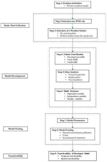
Figure 1.
A diagram of the methodology adopted at each step.
3. Study Data
Traffic and weather data were the two data sources used in this study. Alberta Transportation (AT) is a provincial agency that builds and rehabilitates the transportation infrastructure in the province of Alberta and collects traffic data from the weigh-in-motion (WIM) system. AT has been continuously collecting vehicle information data such as axle load, the speed of the vehicle, and the date and time of travel through six WIM sites installed on Alberta highway network from July 2004. Five years of the data spanning from 2005 to 2009 was used to develop the winter-weather traffic models, and an additional 2010 data set is used to test their transferability. Although AT has been continuously collecting WIM data at the same sites used for this research, the data of 2010 were the most recent data for which vehicle classification, weather, and traffic data were available to us. Therefore, the data for the year 2010 were used for assessing the temporal transferability of the weather traffic model.
Environment Canada has about 8,000 weather stations installed over the country, out of which 598 are operating in the province of Alberta, which collect climatology data daily. The weather parameters recorded by weather station includes rainfall (mm), snowfall (cm), mean temperature (°C). Environment Canada’s National Climate Data Archive was used to extract the weather data for this study. The weather data shows that snowfall and cold temperatures continue to be recorded from November to March every year, so these five months were considered as the winter season and used for modeling. As a result, a total of 510 days were selected for modeling for the five-year study period.
It is very important to designate a weather station that can adequately represent the climatic conditions of the WIM site. To pursue this, a two-step process was developed. The first step involves identifying all the weather stations around the WIM site. For this purpose, a base map with the help of a geographic information system (GIS) was developed which included all the 598 weather stations and the study WIM sites. The second step involved locating weather stations installed within a radius of 16–24 km from the WIM site. The determination of this effective distance is based on the results of previous studies [17,21,22]. These studies indicated that climatic conditions within a distance of 16–24 km from weather station could be considered homogeneous. Table 1 summarizes weather stations that are closest to the WIM site and shows the amount of missing weather data of each weather station. The Edmonton Woodbend weather station at Hwy 44 had missing weather data for 25 days and the Monarch weather station at Hwy3 had missing weather data for 100 days. The Shining Bank weather station at Hwy 16 had missing weather data for 157 days. Other weather stations associated with Leduc Hwy 2A, Leduc Hwy 2, and Red Deer Hwy 2 had no missing data. According to the recommended distance criteria and the integrity of weather data, modeling proceeded with three WIM sites which satisfied the distance standard and had no missing weather data.

Table 1.
Information on WIM Sites and their associated weather station.
4. Model Development
4.1. Vehicle Classification
The first task of the model building process began with classifying vehicles using vehicular records obtained from the study WIM sites. Vehicle classification was conducted in a three-step procedure. The first step involved segregating vehicular records into two classes: complete data records (CDRs) and incomplete data records (ICDRs) according to whether full information for classification exits or not. The second step involved developing visual basic (VB) computer code that classifies vehicles into 13 subclasses from CDRs using information about axle spacing and the number of axles based on the scheme F developed by Maine Department of Transportation under the contract by of Federal Highway Administration (FHWA) [23]. As the third step, the vehicular records in the ICDRs were distributed proportionally to the traffic volumes of each vehicle classes classified in the second step. Due to the low amount of truck traffic, and other subclasses, the 13 vehicle classes were aggregated into three vehicle classes: total traffic, passenger car traffic, and truck traffic.
4.2. Preliminary Data Analysis
Vehicle classification was followed by preliminary data analysis which was carried out by plotting scatter plots between the independent variables and the dependent variable. Figure 2 shows scatter plots between the dependent variable of observed daily volume factor and the independent variables such as expected daily volume factor (EDVF), snowfall, and temperature for the data obtained at one of the study WIM sites. Observed traffic volume factor, defined as the ratio of total daily traffic to the annual average daily traffic (AADT), is used instead of daily traffic volume to account for annual variations in traffic volume. The EDVF, used as one of the independent variables in this study, is an averaged daily traffic volume factor calculated from historical traffic volume over the five-year study period. The relationship between observed daily volume factor and the EDVF shows a strong positive linear for all three vehicle classes, as shown in Figure 2a,d,g.
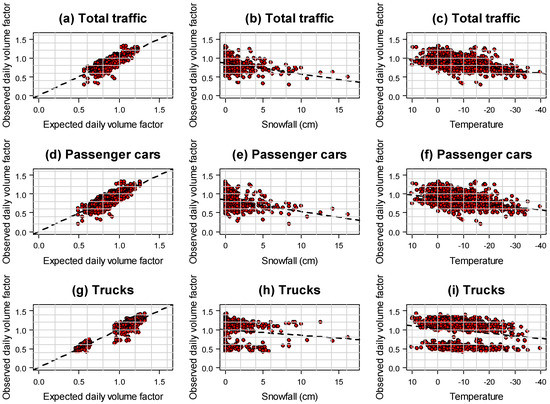
Figure 2.
Scatter plots between dependent and independent variables.
As shown in Figure 2b,e for snowfall and Figure 2c,f for temperature, heavy snowfall, and cold temperature have a negative effect on the total traffic volume and passenger traffic volume. In contrast, truck traffic was affected less by changes in snowfall and temperature, compared to total traffic volume and passenger cars, as shown in Figure 2h,i.
4.3. Traffic Pattern
This section investigates the traffic patterns of passenger car and truck traffic at the three study WIM sites. According to an initial statistic of WIM data, passenger traffic accounted for 92% of the Leduc Hwy 2A site, 84% for Red Deer Hwy 2, and 83% Leduc Hwy 2. Passenger car traffic pattern is very similar to total traffic pattern because of the high share of passenger cars in total traffic volume. The hourly and daily variations in traffic patterns of passenger cars and trucks are shown in Figure 3, Figure 4 and Figure 5 for each of the three WIM sites.
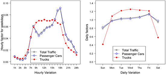
Figure 3.
Typical hourly and daily variations of traffic at Leduc Highway 2A.
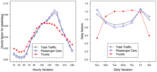
Figure 4.
Typical hourly and daily variations of traffic at Leduc Highway 2.
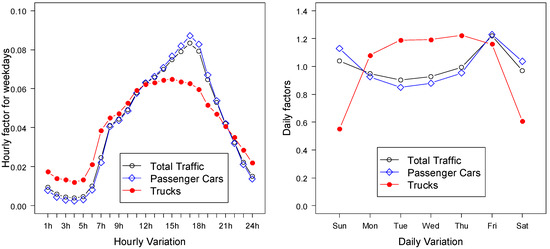
Figure 5.
Typical hourly and daily variations of traffic at Red Deer Highway 2.
Sharma et al. developed a method of classifying highways according to the trip length and purpose of the travel population [24]. The same classification system was employed to classify the highway segments on which the study WIM systems were installed. The common traffic pattern observed at two of the WIM sites, Leduc Hwy 2 (Figure 4) and Red Deer Hwy 2 (Figure 5), is that peak hour traffic in both the morning and evening is not clearly distinguishable. The reason for this is that the highways primarily carry a mix of long-haul inter-regional traffic and therefore can be classified as an inter-regional long-distance route. On the other hand, the WIM site located on Hwy 2A near Leduc (Figure 3) has observed the peak traffic volumes in the morning and evening, and the traffic volume on weekends was reduced compared to weekdays. This highway is primarily responsible for work and business trips originating within commuting areas near the City of Edmonton and can be classified as a regional commuter route.
4.4. Model Development and Testing
To analyze and study the relationship between traffic volume and the weather factors, a dummy variable regression modeling technique was employed. A dummy variable regression model was developed respectively for each of the three WIM sites for total traffic and passenger car, truck traffic volume. In the model specification, EDVF and snowfall are included as two quantitative independent variables and daily mean temperature, categorized into seven classes, is included as a qualitative independent variable. The EDVF used for model calibration was the traffic volume which is averaged over historical traffic volume. The inclusion of this variable in the model specification was responsible for the explanation of the systematic part in traffic volume changes that is repeated periodically solely by the traffic event other than the climate events such as rainfall and snowfall. The systematic part of the traffic volume change can be explained by the EDVF variable, but it cannot explain all the changes. Thus, by including low temperature and snowfall in the model specification, the model can be specified as a system which is capable of capturing the part of random changes in traffic volume due to arbitrary meteorological phenomena. The daily mean temperature used as a dummy variable is classified into seven cold categories with the same 5 °C interval ranging from the baseline category of over 0 °C to CC6 category of below −25 °C. The dummy variable regression model is constructed for all three types of vehicles for all three WIM sites following the formulation given in Equation (1).
where, indicates the observation; indicates estimated value of daily traffic volume factor for each of the three types of vehicle; , and indicate coefficients for each independent variable; = 1 if observation falls in cold category , otherwise 0, and is the error term.
The variables coefficients are estimated for total traffic, passenger car traffic and truck traffic models. Although total traffic is not a different class of vehicles, we considered developing models for it. The rationale behind such a consideration is that most of the earlier studies analyzed the effects of inclement weather conditions on total traffic without any classifications because of the lack of data availability. Permanent traffic counters record only total traffic data, unlike WIM which provides classified traffic count. It would be of benefit to see modeling results of each vehicle class including total traffic to understand how each vehicle class is affected by severe weather conditions compared to the study which considered total traffic, only.
Pearson correlation coefficient () is used to evaluate the overall goodness of fit of the dummy variable regression model. The correlation coefficient is above 99% for all the models, except for the model 3 (Table 2), which implies that the developed models fit well with the sample data. The overall significance of the dummy variable regression model is tested by F-statistics. Results from F-statistics indicate that all the models are statistically significant at the 0.001 level. The result of the T-statistic is presented using the symbol (*) which indicates the significance of the estimated coefficients by the number of it. The incremented F-statistic was used to reject the null hypothesis that the dummy variable regression modelling was not an improvement over the naive model which does not include any dummy variables. The incremental F-statistics justify the inclusion of dummy variables of cold categories at 0.05 (or less than 0.05) level for all models. The estimated coefficients along with model structures are given in the Table 2 for Leduc Hwy 2A, Table 3 for Leduc Hwy 2, and Table 4 for Red Deer Hwy 2.
Table 2.
Daily winter weather regression models with dummy variables at Leduc Hwy 2A.
Table 3.
Daily winter weather regression models with dummy variables at Leduc Hwy 2.
Table 4.
Daily winter weather regression models with dummy variables at Red Deer Hwy 2.
It was found that total traffic and passenger car were affected in statistical terms by cold and snow as observed from the modeling results in Table 2 (models 1 and 2) for Hwy 2A, in Table 3 (models 4 and 5) for Leduc Hwy 2 and in Table 4 (models 7 and 8) for Red Deer Hwy 2. However, the phenomenon is not consistently observed in truck traffic. Truck traffic on Hwy 2A were not found to be statistically affected by temperature and snow as shown in Table 2 (model 3). Interestingly, trucks traveling on Leduc Hwy 2 (model 6) and Red Deer Hwy 2 (model 9) were more vulnerable to temperature and cold than truck traffic on Hwy 2A. It is the consensus through this study that the truck traffic is not influenced by cold temperatures and snowfall as much as passenger car traffic was affected. It is also noted that the variation in truck traffic is affected differently by weather condition according to the road classification of the highway segment. Figure 6, Figure 7 and Figure 8 show scatter plots between the estimated daily traffic factors and the observed daily traffic factors used in the development of the models for the study WIM sites. The degree of accuracy of estimation between the two variables is evaluated by performing regression analysis and is represented in terms of Pearson correlation coefficient of . This value of is presented with the figures to show the overall accuracy of the developed models. Figure 9, Figure 10 and Figure 11 show the marginal variation of traffic volumes with different cold categories for all the three WIM sites. Cold has a different effect on traffic flow depending on the nature of the traffic that the highway is supporting. Overall, truck traffic is observed to be less dependent on the cold category as compared to the passenger car traffic.
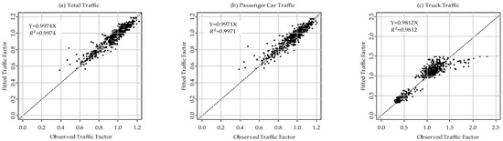
Figure 6.
Fitted dummy variable regression modeling results at Leduc Highway 2A.
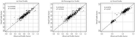
Figure 7.
Fitted dummy variable regression modeling results at Leduc Highway 2.
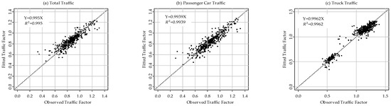
Figure 8.
Fitted dummy variable regression modeling results at Red Deer Highway 2.
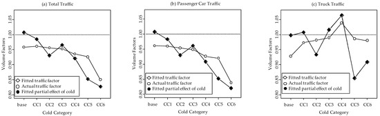
Figure 9.
The marginal effect of cold categories on traffic volume factor at Leduc 2A.
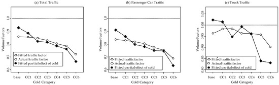
Figure 10.
The marginal effect of cold categories on traffic volume factor at Leduc Highway 2.
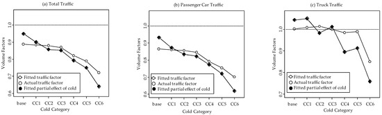
Figure 11.
The marginal effect of cold categories on traffic volume factor at Red Deer Highway 2.
5. Temporal Transferability
It will be of great utility to the transportation agencies if the models developed at one point in time zone can be used at a different time zone. This helps to reduce the effort of data collection and saves both time as well as money. This section aims to test the temporal transferability of the models developed in the previous section. That is, it tests whether a model developed in a one-time frame can be applied to another time frame irrespective of the gap between the development and application of the model. To test the temporal model transferability of the models developed using data spanning from 2005 to 2009, additional WIM data of 2010 was obtained from Alberta Transportation at the same site. To test the accuracy of estimated traffic factors from the transferred model a regression line between the observed and estimated traffic factors is developed and the value of is used as a measure of accuracy. Temporal transferability is tested for both naive winter weather model as well as the dummy variable regression model in order to develop a comparison between the two model types. Another reason to test transferability with two different model specifications is to see if cold categories were not found to be statistically significant for truck traffic and hence, to reach a decision that the estimation of truck traffic might be better with a naive model as compared to a dummy variable model. This could mean that a dummy variable model could be selected as a final model form for passenger car traffic and total traffic whereas a naive model could be selected as a final model specification for truck traffic.
Figure 12, Figure 13 and Figure 14 show the transferability test results for the dummy variable regression model and Figure 15, Figure 16 and Figure 17 show the results for naive winter weather models for the three study WIM sites. The regression line was developed for all the models and the value of is observed to be greater than 0.93 for all the models. A relatively strong value of between observed and estimated traffic factors, indicates that the dummy variable regression model can be temporally transferred between two-time frames and can be used to predict the traffic factors fairly accurately. The accuracy of prediction, , is better with a dummy variable model for total and passenger car traffic (see Figure 12a,b compared to Figure 15a,b and see Figure 13a,b compared to Figure 16a,b) while the naive model gives a slightly better prediction for truck traffic (see Figure 12c compared to Figure 15c and see Figure 14c compared to Figure 17c). In the case of Red Deer Hwy 2, a naive model provides a marginally better performance for the total and passenger car variables (see Figure 14a,b compared to Figure 17a,b). For the Leduc Hwy 2, a dummy variable model provides a little bit better performance for truck traffic (see Figure 13c compared to Figure 16c).
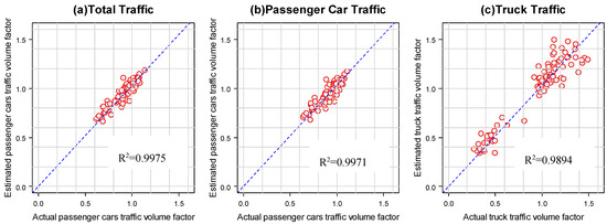
Figure 12.
The accuracy of temporal transferability for dummy variable regression model at Leduc 2A.
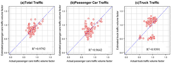
Figure 13.
The accuracy of temporal transferability for dummy variable regression model at Leduc Highway 2.
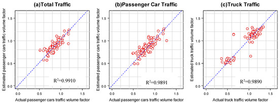
Figure 14.
The accuracy of temporal transferability for dummy variable regression model at Red Deer Highway 2.
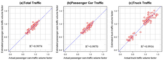
Figure 15.
The accuracy of temporal transferability for naive regression model at Leduc Highway 2A.
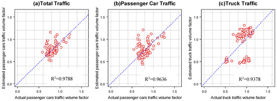
Figure 16.
The accuracy of temporal transferability for naive regression model at Leduc Highway 2.

Figure 17.
The accuracy of temporal transferability for naive regression model at Red Deer Highway 2.
6. Summary and Conclusions
This study focuses on the development of winter weather traffic models with the introduction of dummy variable regression techniques to estimate the changes in traffic volumes for three types of vehicles triggered by adverse winter weather factors such as snowfall and cold temperature. The models in this study are developed with a five-year WIM data spanning from 2005 to 2009. The data was collected at three WIM sites located on major highways in the province of Alberta, Canada. The mixed traffic stream data was classified into three vehicle classes; total traffic, passenger car, and truck traffic according to the purpose of this study. Meteorological data used in this study, daily temperature and snowfall during winter months, was obtained from Environment Canada. Temperature, used as a dummy variable in this study, was classified into seven categories (baseline, CC1~CC6).
The results from winter weather traffic models developed indicate that total traffic and passenger car traffic shows a constant decline with an increase in the amount of snowfall and a decrease in temperature. However, truck traffic is not significantly affected by temperature. It seems that snowfall has an impact on the variation in truck traffic on Leduc Hwy 2 and Red Deer Hwy 2, but it is less compared to the impact on the passenger cars. This is because of the fact that trips carried out by trucks are mostly mandatory trips and cannot be delayed or adjusted even by inclement weather conditions. In the case of passenger cars when drivers encounter an adverse driving environment, various options such as the flexibility of change of departure time, ease of change of travel route, or cancellation of travel may be considered. Conversely, truck drivers often have to travel on a planned rigorous schedule, regardless of weather conditions. This kind of business-oriented travel increases the likelihood that a truck will show a unique driving pattern even in harsh weather conditions.
Temporal transferability of the models has also been evaluated in this study by transferring the developed models to the year 2010. The level of accuracy of the transferability was tested by regression analysis between the estimated values (from the model) and the observed values (from the WIM site). Two different types of model specifications such as the dummy variable regression model and the naive model were tested for the accuracy of predictions in terms of transferability. While the dummy variable regression models showed better accuracy in predicting total traffic and passenger car traffic, naive models showed better accuracy for truck traffic predictions, but the difference was negligible. This negligible difference can be attributed to the fact that truck traffic is relatively unaffected by low temperatures and hence the cold categories (dummy variables) are statistically insignificant for truck traffic.
Author Contributions
The authors confirm contribution to the paper as follows: conceptualization: H.-J.R., S.S.; methodology: H.-J.R., S.S., P.K.S.; software: H.-J.R.; validation: P.K.S., F.A.B., S.S., B.M.; formal analysis: H.-J.R.; investigation: H.-J.R., P.K.S., F.A.B.; resources: O.R.; data curation: H.-J.R.; writing—original draft preparation: F.A.B., P.K.S., H.-J.R.; writing—review and editing: H.-J.R., P.K.S., F.A.B., A.M.K., B.M.; visualization: H.-J.R.; supervision, H.-J.R., P.K.S., S.S.; project administration: S.S., H.-J.R.
Funding
This research received no external funding.
Acknowledgments
Authors are thankful to Alberta Transportation for providing WIM data used for this research.
Conflicts of Interest
The authors declare no conflict of interest.
References
- Keay, K.; Simmonds, I. The association of rainfall and other weather variables with road traffic volume in Melbourne, Australia. Accid. Anal. Prev. 2005, 37, 109–124. [Google Scholar] [CrossRef] [PubMed]
- Sabir, M.; van Ommeren, J.; Koetse, M.J.; Rietveld, P. Impact of Weather on Daily Travel Demand; 2060163; Department of Spatial Economics, VU University of Amsterdam: Boelelaan, The Netherlands, 2010. [Google Scholar]
- Akin, D.; Sisiopiku, V.P.; Skabardonis, A. Impacts of weather on traffic flow characteristics of urban freeways in Istanbul. Procedia-Soc. Behav. Sci. 2011, 16, 89–99. [Google Scholar] [CrossRef]
- Hranac, R.; Sterzin, E.; Krechmer, D.; Rakha, H.; Farzaneh, M. Empirical Studies on Traffic Flow in-Inclement Weather; Summary Report; U.S. Department of Transportation, Federal Highway Administration: Washington Colombia, DC, USA, 2006; FHWA-WOP-07-073; p. 108.
- Maze, T.H.; Agarwal, M.; Burchett, G. Whether weather matters to traffic demand, traffic safety, and traffic operations and flow. Transp. Res. Rec. 2006, 1948, 170–176. [Google Scholar] [CrossRef]
- Kilpeläinen, M.; Summala, H. Effects of weather and weather forecasts on driver behaviour. Transp. Res. Part F Traffic Psychol. Behav. 2007, 10, 288–299. [Google Scholar] [CrossRef]
- Smith, B.L.; Byrne, K.G.; Copperman, R.B.; Hennessy, S.M.; Goodall, N.J. An investigation into the impact of rainfall on freeway traffic flow. In Proceedings of the 83rd Annual Meeting of the Transportation Research Board, Washington, DC, USA, 11–15 January 2004. [Google Scholar]
- Andrey, J.; Mills, B.; Leahy, M.; Suggett, J. Weather as a chronic hazard for road transportation in Canadian cities. Nat. Hazards 2003, 28, 319–343. [Google Scholar] [CrossRef]
- Stern, A.D.; Shah, V.; Goodwin, L.; Pisano, P. Analysis of weather impacts on traffic flow in metropolitan Washington DC. In Proceedings of the 19th International Conference on Interactive Information and Processing Systems (IIPS) for Meteorology, Oceanography, and Hydrology, Long Beach, CA, USA, 3–9 February 2003. [Google Scholar]
- Al Hassan, Y.; Barker, D.J. The impact of unseasonable or extreme weather on traffic activity within Lothian region, Scotland. J. Transp. Geogr. 1999, 7, 209–213. [Google Scholar] [CrossRef]
- Liu, C. Understanding the Impacts of Weather and Climate Change on Travel Behaviour. Ph.D. Thesis, KTH Royal Institute of Technology, Stockholm, Sweden, 2016. [Google Scholar]
- Badoe, D.A.; Steuart, G.N. Urban and travel changes in the Greater Toronto Area and the transferability of trip-generation models. Transp. Plan. Technol. 1997, 20, 267–290. [Google Scholar] [CrossRef]
- Doubleday, C. Some studies of the temporal stability of person trip generation models. Transp. Res. 1977, 11, 255–264. [Google Scholar] [CrossRef]
- Ashford, N.; Holloway, F.M. Time stability of zonal trip production models. J. Transp. Eng. 1972, 98, 79–806. [Google Scholar]
- Caldwell, L.C., III; Demetsky, M.J. Transferability of trip generation models. Transp. Res. Rec. 1980, 751, 5662. [Google Scholar]
- Holguín-Veras, J.; Sánchez-Díaz, I.; Lawson, C.; Jaller, M.; Campbell, S.; Levinson, H.; Shin, H.-S. Transferability of Freight Trip Generation Models. Transp. Res. Rec. J. Transp. Res. Board 2013, 2379, 1–8. [Google Scholar] [CrossRef]
- Datla, S.; Sharma, S. Impact of cold and snow on temporal and spatial variations of highway traffic volumes. J. Transp. Geogr. 2008, 16, 358–372. [Google Scholar] [CrossRef]
- Datla, S.; Sahu, P.; Roh, H.-J.; Sharma, S. A Comprehensive Analysis of the Association of Highway Traffic with Winter Weather Conditions. Procedia Soc. Behav. Sci. 2013, 104, 497–506. [Google Scholar] [CrossRef]
- Roh, H.J.; Sharma, S.; Sahu, P.K.; Datla, S. Analysis and modeling of highway truck traffic volume variations during severe winter weather conditions in Canada. J. Mod. Transp. 2015, 23, 228–239. [Google Scholar] [CrossRef]
- Roh, H.-J.; Sahu, P.K.; Sharma, S.; Datla, S.; Mehran, B. Statistical Investigations of Snowfall and Temperature Interaction with Passenger Car and Truck Traffic on Primary Highways in Canada. J. Cold Reg. Eng. 2016, 30, 04015006. [Google Scholar] [CrossRef]
- Datla, S.; Sharma, S. Variation of Impact of Cold Temperature and Snowfall and Their Interaction on Traffic Volume. Transp. Res. Rec. J. Transp. Res. Board 2010, 2169, 107–115. [Google Scholar] [CrossRef]
- Andrey, J.; Olley, R. The relationship between weather and road safety: past and future research directions. Climatol. Bull. 1990, 24, 123–127. [Google Scholar]
- Wyman, J.H.; Braley, G.A.; Stevens, R.I. Field Evaluation of FHWA Vehicle Classification Categories—Maine Department of Transportation. Executive Summary; Federal Highway Administration: Washington Colombia, DC, USA, 1985.
- SHARMA, S.C.; Lingras, P.J.; Hassan, M.U.; Murthy, N.A.S. Road classification according to driver population. Transp. Res. Rec. 1986, 1090, 61–69. [Google Scholar]


© 2019 by the authors. Licensee MDPI, Basel, Switzerland. This article is an open access article distributed under the terms and conditions of the Creative Commons Attribution (CC BY) license (http://creativecommons.org/licenses/by/4.0/).