Article

Simulating 10,000 Years of Erosion to Assess Nuclear Waste Repository Performance

1
Earth and Environmental Sciences, Los Alamos National Laboratory, Los Alamos, NM 87545, USA
2
Neptune and Company, Los Alamos, NM 87544, USA
*
Author to whom correspondence should be addressed.
Geosciences 2019, 9(3), 120; https://doi.org/10.3390/geosciences9030120
Submission received: 12 January 2019 / Revised: 5 March 2019 / Accepted: 5 March 2019 / Published: 8 March 2019
(This article belongs to the Special Issue Soil Hydrology and Erosion)

Abstract

:
Long-term environmental performance assessments of natural processes, including erosion, are critically important for waste repository site evaluation. However, assessing a site’s ability to continuously function is challenging due to parameter uncertainty and compounding nonlinear processes. In lieu of unavailable site data for model calibration, we present a workflow to include multiple sources of surrogate data and reduced-order models to validate parameters for a long-term erosion assessment of a low-level radioactive nuclear waste repository. We apply this new workflow to a low-level waste repository on mesas in Los Alamos National Laboratory in New Mexico. To account for parameter uncertainty, we simulate high-, moderate-, and low-erosion cases. The assessment extends to 10,000 years, which results in large erosion uncertainties, but is necessary given the nature of the interred waste. Our long-term erosion analysis shows that high-erosion scenarios produce rounded mesa tops and partially filled canyons, diverging from the moderate-erosion case that results in gullies and sharp mesa rims. Our novel model parameterization workflow and modeling exercise demonstrates the utility of long-term assessments, identifies sources of erosion forecast uncertainty, and demonstrates the utility of landscape evolution model development. We conclude with a discussion on methods to reduce assessment uncertainty and increase model confidence.

1. Introduction

Conducting a long-term performance assessment (PA) of radioactive waste storage facilities is a necessary step to ensure that facilities meet safety requirements [1], provide objective input to regulatory decision-makers [2], and assuage public perception of radioactive storage [3]. For U.S. Department of Energy (DOE) sites, Order 435.1 [1] requires that radioactive waste be managed in a manner that protects public health and safety and the environment, along with providing a PA for 1000 years for low-level nuclear waste and up to 100,000 years for high-level nuclear waste. These comprehensive assessments require a broad application of geosciences including erosion analysis. Long-term erosion can play a significant role in the PA, as erosion processes can expose buried material and transport the material offsite to potential contaminant receptors within the 1000- and 100,000-year timeframes. However, given the long-term timeframes and complexity of nonlinear erosion, careful examination of model assumptions, parameterization, and results is essential to understanding how uncertainty and model performance may affect the PA [2]. Here we present a detailed description of how an erosion model was parameterized and the assumptions used, with results for an extended analysis of a low-level nuclear waste site to better understand the strengths and weaknesses of the erosion component of a PA. This work is the culmination of a multi-decadal effort to develop a robust erosion PA by optimizing the inclusion of surrogate site and model data, which serves as an example for how other PAs involving long time scales can be implemented.
Radioactive waste at Los Alamos National Laboratory (LANL) is disposed at Material Disposal Area G (MDA G). Area G is located on LANL property on the Pajarito Plateau between the communities of Los Alamos and White Rock (Figure 1). Waste is placed in large rectangular pits, numbered 1–39, and cylindrical shafts within MDA G. DOE facilities that received waste after 26 September 1988, which includes MDA G, are required to prepare and maintain a site-specific radiological PA. These sites are also required to conduct a composite analysis (CA) that accounts for the cumulative impacts of all waste that has been and will be disposed of at the facilities; this includes other sources of radioactive material that may interact with these facilities. Erosion estimates are used within the PA for human health risk assessments that account for rates of soil loss through time across low-level nuclear waste disposal regions. These losses are used to update the thickness of the surface soil, the engineered cap, and waste layers through time, as well as the associated risk of exposure. The PA/CA is required to assess the radiological impacts of the waste over a 1000-year compliance period. This 1000-year period begins after the expected site closure date (originally 2047 but recently modified to 2035 for MDA G).
The SIBERIA landscape evolution model (LEM) [4,5,6] is in a class of erosion models that are designed to simulate the development of drainage networks and depositional features such as alluvial fans. LEMs contrast to sediment transport models, such as the Water Erosion Prediction Project (WEPP) [7], KINEROS [8], and the Hillslope Erosion Model (HEM) [9], because LEMs represent whole landscape features. LEMs further attempt to forecast how landscape features evolve at geomorphic time scales by representing the lowering of ridges, the incision or infilling of valleys and hollows, and the development of gullies and fans due to erosion, sediment transport, and material deposition [10]. These processes alter and deform the terrain to produce an evolving three-dimensional (3D) representation of the landscape. For PAs such as MDA G, SIBERIA estimates spatially variable rates of sediment transport and estimates spatial and temporal changes in the thickness of the protective cover material.
The application of LEMs is largely dependent on the time scale in question. LEMs are originally developed to represent average landscape evolution for periods of time long enough to where climate has changed many times and average landscape behavior may emerge [10,11]. This is estimated to be approximately 100,000 to 10,000,000 years. Clearly, the time scales at which LEMs are developed presents a problem for model validation [12]. Nevertheless, validation at shorter timescales (tens to hundreds of years) has shown LEMs to be robust in representing key landscape shaping processes (e.g., [13]). Therefore, some LEMs, specifically SIBERIA, have been used to simulate erosion from abandoned and operating mining sites (e.g., [14,15,16,17]) and have been used to simulate erosion for 1000 years [12]. However, questions remain regarding model performance in time periods between near-term forecasts (1000 years or less) and the extended-term 100,000-year forecast when average behavior emerges.
Previous PAs for MDA G used SIBERIA to evaluate the impacts of surface erosion on the performance of a final cover design to 1000 years [18,19], which spans the required PA compliance period [1]. However, it is acknowledged that radioactive material may interact with the surrounding environment beyond the passive institutional control period of 1000 years. In fact, simulations for groundwater transport scenarios have been conducted out to 100,000 years in order to evaluate full residence time distributions for breakthrough at the compliance point for the groundwater pathway [20]. The work reported here extends the erosion analysis to 10,000 years to gain critical insight into the potential for long-term erosion and to better understand the limitations of the long-term erosion modeling analysis. While few studies have used LEMs to assess long-term erosion for the purpose of assessing the performance of waste repository and mine reclamation sites, those that have [21,22] provide critical information on model performance and uncertainty.

2. Materials and Methods

This extended erosion analysis builds on more than 15 years of modeling work at MDA G [18,19,23]. The initial model development and parameterization to employ SIBERA to the radioactive waste repository was described in 2005 by Wilson et al. [18]. This work was then updated in 2010 by French and Crowell [19] to include unique erosive properties of underlying material as erosion encounters bedrock material. In 2013 [23], a sensitivity analysis was conducted using the parameterized SIBERIA model to investigate a range of erosive properties for three erosion scenarios—low, moderate, and high—that differ in terms of runoff volume and ground surface characteristics. These scenarios were defined, in part, using average properties of 17 hillslope profiles located within, or immediately adjacent to, the MDA G site. The sensitivity analysis only simulated 1000 years from the present, whereas we now extend that analysis out to 10,000 years. Calculations of erosion provide estimates of mass removed; however, at this time, the analysis has not been carried through to calculate exposure or dose impacts in the PA/CA site model.

2.1. Modeling Background

SIBERIA considers erosion as a function of slope and the contributing area of runoff within a landscape feature. This approach allows SIBERIA to employ the “geomorphically effective event assumption”, which assumes that, at long time scales, erosion can be represented as a steady process. Runoff is considered as a constant low-magnitude process that shapes the landscape. The 3D forecast of drainage networks and SIBERIA’s computational efficacy enable long-time-scale simulations that are necessary for long-term erosion forecasts at MDA G.

2.1.1. Governing Equations

SIBERIA simulates erosion and sediment transport over a landscape represented as a gridded digital elevation model (DEM). The erosion and sediment simulation deforms the model landscape over time. Sediment transport through each grid cell is calculated with an expression of the form:
Qs = BAmSn + DzS
where:
  • Qs = sediment flux through a grid cell (kg/m width)
  • B = a coefficient that establishes the rate of sediment transport
  • A = area that contributes to runoff (m2)
  • S = terrain slope (m/m)
  • m, n = exponents used to define how sediment yield depends on runoff contribution
  • area (A) and slope (S) for a given cell
  • Dz = diffusion coefficient (kg/m width)
The exponents m and n affect the long-term form of the landscape, while the rate at which the landscape evolves through erosion is determined by the parameter B. The value of B is related to the short-term, event-based sediment flux through a scaling relationship with mean annual peak discharge and event duration provided in Willgoose [24] and Willgoose et al. [5]. Dz is the diffusion transport coefficient and is a spatially constant Fickian diffusion term that is intended to represent the long-term average of the cumulative effects from hillslope soil creep, rain splash, and rock slide. Over time, Dz will have a strong influence on the shape of the landform; a high Dz will lead to soil movement from upslope areas, resulting in high erosion fluxes.
Willgoose et al. [25] developed a relationship between the local slope and contributing area with the form:
S = cA−α
where c is a constant and the scaling coefficient is:
α = (m − 1)/n.
This relationship defines which processes dominate local erosion, the diffusion processes of soil creep, and rain splash or advection-dominated transport in channels. As described in Willgoose et al., [25] small contributing areas, typical of the upper portions of hillslopes, are dominated by diffusion transport, whereas large contributing areas are dominated by advection-dominated erosion. Moving along a gradient of increasing contributing area, an arc in the surface slope reflects the dominant processes at play. When the contributing area and slopes are small, diffusion processes of creep dominate sediment movement. High surface slopes occur at the boundary between diffusion- and advection-dominated sediment transport, and as slopes diminish within channels an increased contributing area produces a larger flux of runoff to drive advection = dominated erosion.

2.1.2. Model Assumptions

Computational efficiency, and therefore the ability to simulate long time scales, relies on the “geomorphically effective runoff event” assumption. The assumption is that a single steady runoff rate is equivalent to a series of natural runoff events in terms of average sediment movement and geomorphic landform evolution. The geomorphically effective runoff event assumption has been justified by deriving a time-averaged sediment transport equation in which the representative discharge is equal to the mean annual peak discharge [24]. However, the resulting representative discharge is noted as approximate and the variability of runoff is lost [26]. Instead of variable runoff intensities, the representative discharge for each cell is calculated as a function of the contributing drainage area and applied constantly through time. While this assumption allows for efficient computational time and long simulated time scales, the simplified flow propagation means that the effects of differential flow depths and varied flow velocities are not represented.

2.2. Methods

2.2.1. Model Parameterization and Validation

Building the MDA G erosion modeling framework necessitates a complex workflow to provide SIBERIA with realistic model parameters. If direct data are available, SIBERIA can be parameterized directly using long-term rainfall, runoff, and sediment yield data. This is not the case for MDA G and thus surrogate sites and reduced-order models were necessary for parameter estimation. Figure 2 shows the complete workflow for the MDA G erosion modeling framework. The majority of this section focuses on Branch 1, the steps that incorporate rainfall/runoff data to parameterize B, m, and n, and provide an initial estimate for Dz, as it is the most complicated and likely the largest source of model uncertainty. Section 2.2.2 briefly discusses Branch 3, the assignment of the depth and location of bedrock layers and engineered armor in the form of placed boulders around the rim of the mesa. This is followed by a discussion of Branch 2, incorporating the central MDA G landform using a DEM.
To manage the workflow shown in Figure 2, including the stand-alone numerical codes used to parameterize SIBERIA, the entire workflow was streamlined using the Model Analysis Toolkit (MATK) Python module (http://matk.lanl.gov), which allows for all surrogate models and a SIBERIA forward run to be performed without manually transferring data. Each model run and associated parameters values are stored for reference and tracked by ensemble number. In addition, MATK allows for parallel simulations in order to assess parameter sensitivity or uncertainty.
Values for the parameters B, m and n in SIBERIA were developed using the Infiltration and Runoff Simulation (IRS) model, version 9 [27], and the HEM sediment transport model [9]. To predict runoff depth from a slope for a given storm, the IRS model is parameterized with information including soil texture class (e.g., loam and sandy loam), and canopy and ground cover. The runoff is then used as input for the HEM, which also includes percent vegetation cover and soil information to estimate sediment production along a set of terrain profiles. Finally, SIBERIA parameters B, m and n are calibrated using sediment flux output from eight simulated HEM slopes ranging from 2% to 16% slopes as a calibration target.
The timing and intensity of the precipitation falling on the disposal site plays an important role in determining the rates and patterns of erosion at MDA G. SIBERIA applies an average annual rainfall event and the geomorphically effective runoff event when simulating landscape evolution. This modeling approach requires the definition of a rainfall event and resulting runoff event which, when applied annually to the site, projects sediment yields that are assumed to be similar to those associated with a series of storms that vary in intensity and duration. Calibrating to average annual events rather than specific storm events can effectively parameterize LEM to the century-millennia time scale [13].
A storm with a 2.33-year return period is frequently taken to represent a mean annual event, since this is the corresponding recurrence period for early flood frequency modeling based on the Gumbel statistical distribution [28,29]. To constrain erosion rate uncertainty, the SIBERIA modeling conducted in 2005 and 2010 adopted rainfall events for MDA G with return periods of 2 and 5 years [16]; these return periods bracket the 2.33-year storm generated from the National Oceanic and Atmospheric Administration (NOAA) Atlas 14 [30] for the semiarid southwest. The use of these return periods was further supported by data collected over approximately 16 years from an analog rangeland site at the Santa Rita Experimental Range in Arizona [31], where 16-year average sediment yields were similar to those observed for storms having a return period between 2 and 5 years [18] (Table 1).
The NOAA Atlas 14 [30] was also used to parameterize the characteristic storm used to estimate runoff in the IRS. The characteristic storm was 6 h long with 29.5 mm total rainfall. The IRS represents a variation of rainfall intensity over the duration of the storm, with the peak set in the middle of the 6-hour period and a ratio of peak rainfall intensity to average intensity set at 17.1, meaning that for a brief period the rainfall intensity was 84 mmh-1.
The canopy and ground cover characteristics simulated in the IRS were used to distinguish between low-, moderate-, and high-erosion scenarios. They were defined, in part, using information collected from the 17 hillslope profiles shown in Figure 3. Field measurements conducted along these profiles quantified hillslope length and slope, and canopy and ground cover fractions (Table 1).
Canopy cover includes anything that may intercept a raindrop before it hits the ground surface, including branches, leaves, stems, and other obstructions. Ground cover was recorded if the soil surface was covered by rock, plant litter, plant basal stem, or other objects that shield the soil or obstruct flow along the profile. Each profile was divided into at least four segments based on changes in slope and ground cover, with each segment sampled uniformly at least 20 times.
Eleven of the 17 hillslope profiles occur outside of the MDA G site and are similar insofar as they are located in relatively undisturbed piñon-juniper woodland. Six hillslopes are inside the MDA G site. Ground cover generally consists of plant litter, gravel or small rocks, basal stems of forbs and grasses, and biological soil crust pedicles. The 17 hillslope profiles located in and around MDA G provide representative low, medium, and high vegetation cover, and include profiles that have been irrigated to reestablish vegetation following disposal disturbance.
Soil properties also play a significant role in determining erosion potential. The IRS and HEM modeling conducted to generate reference fluxes for parameterizing SIBERIA initially used sandy loam characteristics. The particle size distribution of this material is analogous to that of crushed tuff [32], which is the standard material used at MDA G for fill, daily cover of waste, and operational closure caps. The dominant soil unit mapped atop mesas of the Pajarito Plateau is the Hackroy Sandy Loam. Additionally, the engineered cover design adopted for the PA/CA includes a 6% clay admixture to increase strength and decrease infiltration while minimizing compaction [33]. An additional suite of the IRS and HEM simulations was performed using characteristics of a loam soil to include the effects of the additional clay content. HEM assigns an erodibility factor of 2.31 to a sandy loam and 1.84 to a loam [9].
Rainfall–runoff simulations were conducted with the IRS model for the 17 hillslope profiles using the rainfall event return periods and soil properties discussed above. The results of the modeling, updated in 2010, are summarized in Table 2. The lowest projected runoff is associated with the 2-year storm and a sandy loam soil, and the highest with the 5-year storm and a loam soil. The runoff projections for loam were generally greater than those estimated for sandy loam; runoff was greatest for the 5-year return period regardless of soil type.
The runoff projections as a function of canopy and ground cover developed using the IRS model are discussed in Crowell [23]. The IRS simulations show that runoff decreases when ground cover or canopy cover increases. Ground cover works to slow runoff by disrupting overland flow, and canopy cover provides additional storage for incoming precipitation. Reducing flow from increased ground and canopy cover fractions tends to promote increased infiltration.
Soon after site closure, ground cover fraction close to 100% may develop because of the initial fertilizer and soil amendments to be applied in order to establish forbs and grasses [33]. However, it is expected that over time the site will transition from grassland to woodland where canopy and ground cover fractions are expected to resemble conditions reported in Table 3.
The low-, moderate-, and high-erosion scenarios were assigned on the basis of the results shown in Table 2; the characteristics of the three scenarios are summarized as input into the IRS and HEM in Table 3. Interestingly, the SIBERIA parameterizations from this model development exercise are similar to other studies evaluating erosion from mining sites [15,16]. The low-erosion scenario was defined as one in which the final cover consists of sandy loam, supports a healthy plant community, and is subject to the less severe 2-year rainfall event. The moderate-erosion scenario assumes a cover of sandy loam, less canopy cover, and a 5-year rainfall event. The runoff predicted for this configuration slightly exceeds that estimated for a loam cover subject to a 2-year storm. The high-erosion scenario assumes poor plant cover, a loam soil characterized by increased runoff, and the more severe rainfall event. The corresponding calibrated SIBERIA parameters fitted to the eight simulated HEM slopes for the low-, moderate-, and high-erosion rates shown Table 3.
The low-, moderate-, and high-erosion scenarios were assigned on the basis of the results shown.

2.2.2. Initial Domain Landform

Following Branch 2 in the model workflow illustrated in Figure 2, a 2-m resolution DEM for MDA G that includes the engineered final cover shape is used to assign the initial landform shape and elevation (Figure 4a). Figure 4b shows the approximate thickness of non-native material (both cover and additional fill above bedrock outside the pit areas) that is expected to be present above the bedrock surface following the construction of the final cover. The estimated thickness of non-native material does not account for clean fill placed in the waste pits. The geometry of the containment structures follows the sloping elevation of the bedrock, where waste can be filled to 1 m below the lowest point along the bedrock rim of the disposal unit. Waste within the disposal unit is then filled even to the respective lowest point. The engineered cover will provide a minimum of 2–3 m cover depth over filled waste pits and shafts, while portions of the axis of the final cover may attain thicknesses of 10 m above bedrock, and additional fill is placed in the main, southeast side canyon. The final cover will be engineered to limit plant and animal intrusion into waste and to reduce the infiltration of water into the waste to minimize radionuclide transport to the regional aquifer. The reduction of infiltration will increase surface runoff, and therefore increase the erosive force to form gullies in the engineered final cover.
Using the updated version of SIBERIA (v8.33), a bedrock layer is now included in the model domain shown in the workflow steps outlined in Branch 3 (Figure 2). The top of the bedrock layer is designated by an estimated bedrock surface (Figure 4c), and its thickness is represented as an approximately 100-m layer down to an elevation of 1900 m. Waste pits are etched into the bedrock down to the pit basement (bottom) elevation for the SIBERIA calculations (Figure 4c). A ring of riprap armoring that is 0.6 m in depth and variable width, as shown in Figure 4d, is placed around the mesa to prevent excessive head cutting initiating along the mesa edge. The bedrock and armor are assigned the same reduced erodibility properties by setting B two orders of magnitude lower than is used for the final cover material.

2.2.3. Model Simulations

The SIBERIA modeling, conducted in 2005 [18], in 2008 [34], and in 2010 [19] using similar parameters and for this study, projects 1000-year erosion rates for the low-, moderate-, and high-erosion scenarios. The purpose of the current analysis is to evaluate erosion to 10,000 years at MDA G for the low-, moderate- and high-erosion scenarios using the parameters listed in Table 3.
An additional model update was used that implements the Dinfinity flow direction algorithm [6,35]. The Dinfinity algorithm calculates the steepest down-slope direction and directs sediment flow based on eight triangular facets in a 3 × 3 cell window. Sediment flow is then partitioned to a maximum of two neighboring cells based on the flow direction calculation. In contrast, the original formulation used a D8 formulation where flow is directed into only one of the eight adjacent cells. By switching to the Dinfinity algorithm, sediment flow more precisely follows the terrain, resulting in (1) increased convergent flow, which affects channel erosion, and (2) gradually changing flow runoff and sediment flux direction at a given location over time. The D8 flow algorithm leads to linear channel formation, whereas the Dinfinity formulation leads to more natural, feathered, and varied channel formation.

3. Results

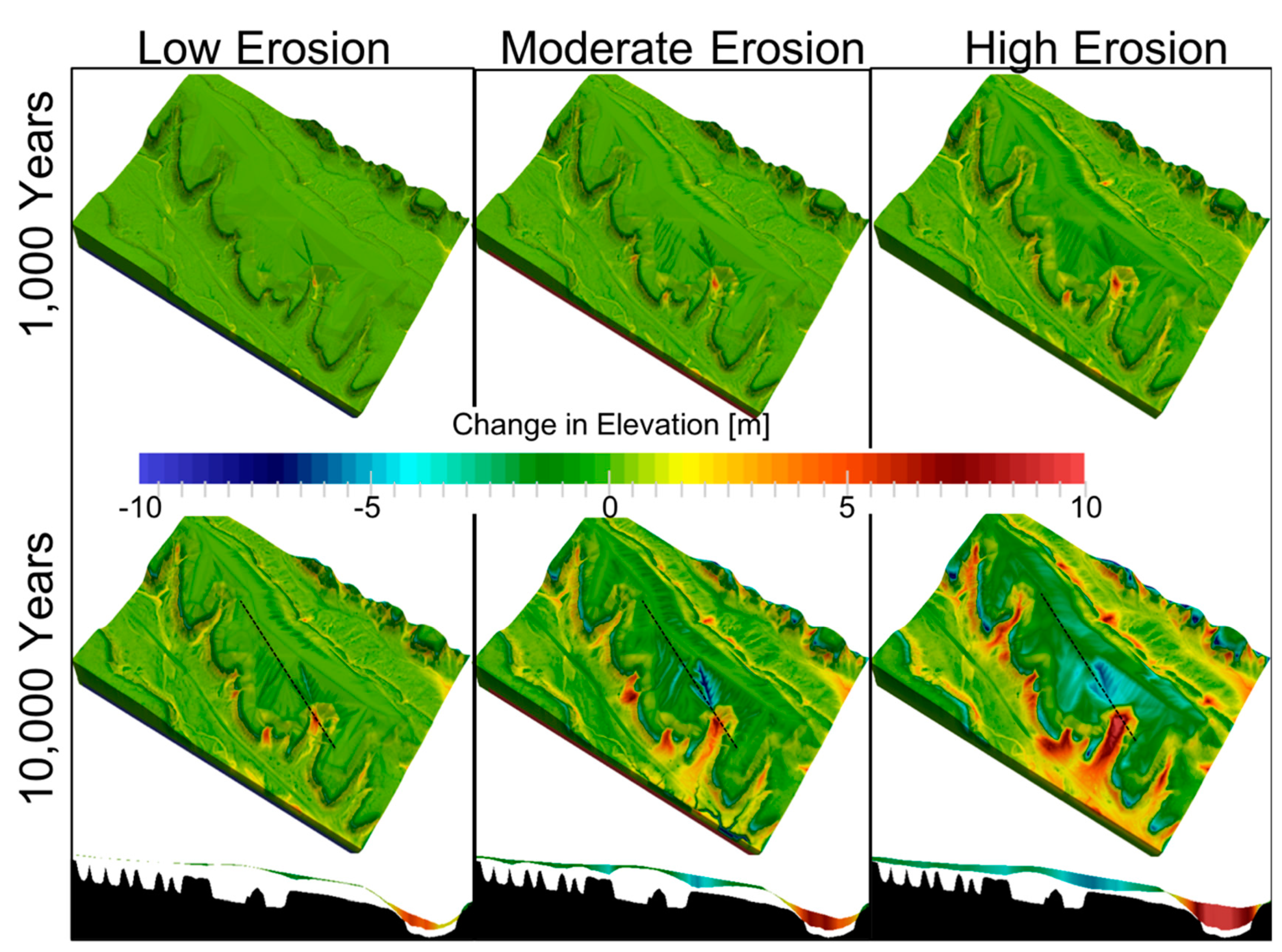
3.1. 10,000-Year Erosion Analysis

As expected, substantially more erosion is observed over the 10,000-year simulations than for the 1000-year simulations (Figure 5). Both the 10,000-year moderate- and high-erosion scenarios have localized areas with approximately 10 meters maximum loss of elevation on the mesa. Interestingly, the long-term low-, moderate-, and high-erosion scenarios express vastly different landscape evolutions. The long-term, high-erosion scenario, which uses the highest diffusion coefficient (Dz) (Table 3), results in a general smoothing of the landform and a loss of cover material by erosion over large swaths on the mesa. Non-intuitively, the moderate-erosion scenario shows the deepest gully formation, with only a moderate overall lowering of the landscape elevation. The moderate-erosion scenario also has the lowest Dz (Table 3) and thus has limited diffuse erosion across the landscape. The low Dz when combined with a moderate B parameter value (Table 3) exacerbates gully formation. The low-erosion scenario with low B and Dz (Table 3) has the lowest long-term erosion and minimal gully formation.
The changes in elevation from the original surface elevation after 10,000 years for the low- and high-erosion cases are shown in Figure 6. These figures illustrate the loss of cover and fill material from the mesa and the deposition of material into the neighboring side canyons. The low-erosion scenario indicates that only a few waste pits, located in the southern central portion of MDA G, will lose up to 1.5 m of cover material, while little (<0.5 m) to no loss occurs over much of the site after 10,000 years. One small gully between 1.5 and 2.5 m in depth is projected to bisect a single pit (Figure 6). In contrast, the high-erosion scenario shows that much of the site will lose between 1.5 and 2.5 m of cover material, with some of the southern central portion of MDA G losing between 2.5 and 5 m of the cover material (Figure 6), but virtually zero bedrock material is eroded. Additionally, the high-erosion case projects that localized areas near the large southeastern side canyon that cuts into the masa may experience greater than 5 m of cover and fill loss. However, it should also be noted that the locations with the highest erosion are either near the crest of the final cover or co-located with a large gully with planned fill, with both locations having cover material that is approximately 10 m deep.
Figure 7 shows the resultant changes in “cover thickness above bedrock” for the high- and low-erosion scenarios. As described previously, this thickness is estimated to include the non-native material above bedrock (i.e., the engineered cover and clean fill outside the pit areas) within the riprap armor. To estimate the remaining thickness, the elevation of the bedrock used in SIBERIA was subtracted from the simulated cover elevation. To estimate the original bedrock surface across pit locations, the locations were filled by interpolating the elevations around the pits using a triangulated network of known points. Because both the initial thickness of the material above bedrock (Figure 4b) and the changes in elevation due to erosion (Figure 6) are highly variable, the estimated thickness of material above bedrock remaining at 10,000 years is used to illustrate areas where losses may approach the level of the waste pits. For the low-erosion scenario (Figure 7a) and in areas with pits present, there is a minimum of 1–2 m of cover/fill above bedrock remaining after 10,000 years. For the high-erosion scenario, there are a few places where the cover/fill material is predicted to erode down to the level of the bedrock and complete loss of the overlying cover/fill material will occur. Of the few locations that erode down to bedrock in the high-erosion scenario above the pits, very little, if any, erosion occurs past the bedrock, and the surface remains above the top of waste at 10,000 years as sufficient clean fill below the estimated bedrock grade but above the waste is present. We note that these results are quite uncertain, and the thickness of material above bedrock is estimated, but the simulations provide a general sense of erosion patterns and soil loss across the site.

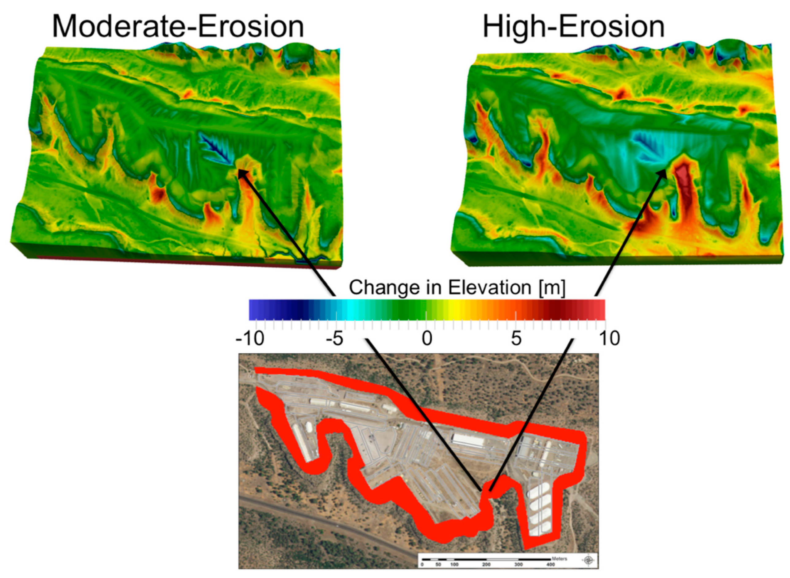
3.2. Impact of Riprap Armor

Despite the large amount of erosion for both the moderate- and high-erosion scenarios, no erosion is predicted to occur around the mesa edges (Figure 8). This indicates that the parameters used in the simulations for the riprap armor prevent erosion along the mesa edges, assuming the riprap will not degrade or fall from the mesa edge. Even though the moderate-erosion case predicts extensive gully formation in the engineered final cover, the mesa edges maintain their initial elevation, which indicates that the gullies do not result from upslope head cutting from the edges of the mesa. Rather, the gullies predicted under the moderate-erosion scenario result from the erosive properties of the cover material and the low Dz.

3.3. Canyon Deposition

Both the moderate- and high-erosion scenarios predict areas of high sediment deposition, 10 m or more after 10,000 years, in the canyon bottoms (Figure 9). The high-erosion scenario, in particular, shows extensive deposition, an indication of the large amount of sediment moved from the mesa top into the canyon bottoms. However, canyon filling is currently not the natural form observed on the Pajarito Plateau, and it is unlikely for the canyon bottoms to fill with 10 m of sediment. The moderate-erosion scenario also shows considerable deposition in the canyon bottom, although the prediction is more consistent with current geomorphology observed on the Pajarito Plateau. As part of the model validation process, simulated deposition in the canyon bottoms was evaluated against the observed geomorphology of the plateau. In cases where canyons were filled with sediment, Dz was decreased to reduce diffusive properties of sediment deposition [18]. Given that the moderate-erosion scenario has the lowest Dz (Table 3) of the three scenarios tested, it would suggest that lowering Dz may result in more realistic erosion and landform projections, but may also reduce the sediment discharge needed to calibrate SIBERIA to the observed hillslope transects (Figure 3). Alternatively, adjusting the m and n parameters to increase advection-driven transport may also reduce sediment deposition within canyon bottom channels. However, a possible source of the excessive canyon bottom deposition is the lack of simulated discrete events, such as large rainfall events, that would normally clear sediment from the canyon bottom, which are not represented within the geomophically effective assumption. Another possibility is that an adjustment of n, the slope sediment yield parameter, may be required for the canyon bottoms.

4. Discussion

The workflow presented here to incorporate multiple sources of surrogate data in the absence of site monitoring due to ongoing site activity provides a robust approach to estimating erosion for a low-level nuclear waste repository. By optimizing model development with multiple avenues for data inclusion, updates to parameter values can be incorporated as site uncertainty is reduced. This study also introduces the state-of-the-art procedures to use available resources and adjacent site knowledge where specific site data are absent. Furthermore, the benefit of documenting such procedures is demonstrated by linking between basic research in LEM development and the physical understanding of erosional processes to a specific need in the environmental management community that is applicable to many sites beyond Area G. For the purposes of engineered site evaluations, specific site characteristics are not always known a priori as specific designs change due to ongoing activities. Here, the low-, moderate-, and high-erosion scenarios used to analyze the impacts of erosion over the 1000-year compliance period are extended to a 10,000-year analysis. This analysis provides a valuable perspective of the long-term model behavior of SIBERIA and of the conceptual model design. It also allows the evaluation of the development of site characteristics beyond the 1000-year compliance period. However, results regarding the depths of erosion should be viewed as uncertain.

4.1. 10,000-Year Forecast Uncertainty

Comparing the results between the low-, moderate-, and high-erosion scenarios after 10,000 years shows significant uncertainty. Not only does the uncertainty span a wide range of total sediment movement off the mesa, but also the resulting land forms in the canyons and on the mesa top are different for each scenario. The high-erosion scenario produces rounded mesa tops and partially-filled canyon bottoms, whereas the moderate-erosion case produces incised gullies and sharp mesa rims. In contrast to both the moderate- and high-erosion cases, the low-erosion case results in relatively little erosion.
Model uncertainty introduced during model parameterization accrues over the simulation to produce significantly different erosion forecasts. Although extensive parameter validation was performed [18], there is substantial initial parameter uncertainty. Moreover, while this initial parameter uncertainty may appear small (Table 3), over the course of 10,000-year simulations, the differing parameters exhibit large ranges in possible sediment yields and landscape evolution. The initial parameter uncertainty between the low-, moderate-, and high-erosion scenarios is largely unavoidable as precise parameter values are unavailable. While SIBERIA can be parameterized directly using long-term rainfall, runoff, and sediment yield data, direct erosion measurements are not available for MDA G. This is primarily because the final cover is not in place to study how erosional forces will reshape the cover over time. Therefore, surrogate sites and a reduced-order model were used to provide estimates for parameters used in SIBERIA.
Calibrating SIBERIA to a reduced-order model may result in model inconsistencies over long time scales. The reduced-order model is incapable of resolving the 3D erosion physics necessary to characterize diffusive processes relative to advective erosional processes. The low-, moderate-, and high-erosion scenarios were determined based on the IRS and HEM models, which simulate erosion only on 1D flow paths with uniform slopes. In contrast, SIBERIA simulates erosion across a 3D landscape and represents diffusion-dominated and transport-dominated erosion and deposition processes via a relationship between m and n, which determine the area sediment yield and the slope sediment yield, respectively. In order to parameterize SIBERIA for low-, moderate-, and high-erosion scenarios, the m and n parameters were calibrated to HEM results that again cannot simulate erosional differences between diffusion-dominated and transport-dominated mechanisms. Therefore, while the m and n parameters may provide the best model fit to a short time 1D calibration, they may not remain applicable for longer 3D representations where, over longer time, more channels may form, or alternatively some channels may aggregate through diffusional process such as slope creep and sediment deposition.

4.2. Geomorphically Effective Runoff Event Assumption

As stated previously, SIBERIA relies on the “geomorphically effective runoff event” assumption, which is computationally efficient and key for simulating long time scales because it assumes average, steady-state behavior. However, the assumption may also significantly bias both the 1000- and 10,000-year erosion assessments as these time scales may not reach average climatic behavior [11], and may result in underestimations of total erosion [36]. Furthermore, the excessive canyon sediment deposition shown in Figure 9, which spans low and high gully formation characteristics, suggests that discrete events are needed to maintain the sharp canyon and mesa formation characteristic of the Pajarito Plateau. Likewise, if the model is unable to represent discrete erosion events that tend to clear canyon bottoms from sediment buildup, it is conceivable that discrete erosion events could affect the mesa tops by excluding more energetic events that might lead to, for example, enhanced gully formation.
Additional model bias may be introduced by insufficiently identifying the variability of rainfall and runoff over the simulation time period. Recently, a growing body of literature suggests that erosion and advection-driven transport rates of sediment tend to increase when discharge (runoff) variability increases (e.g., [26,37,38]). The results of the SIBERIA calculations may not properly represent the effect of runoff variability in two ways: first, by not explicitly representing runoff variability, and second, by not parameterizing SIBERIA with long-term data that capture the runoff variability seen in the U.S. southwest. Runoff and erosion data collected over a 16-year period from the Santa Rita Experimental Range analog rangeland site in Arizona [31] were used to support the choice of a 2.33-year storm return period for the simulated mean annual event by providing a bounding range of 2–5 years. It is unlikely that a 16-year analysis captures the rainfall and runoff variability encountered over a 10,000- or even a 1000-year period. Indeed, there is strong evidence for many multi-decadal droughts and wet periods in the past 400 years (e.g., [39,40]) which may surpass the 2- and 5-year return periods used by French and Crowell [19]. Furthermore, the 2.33-year storm return period generated from the NOAA Atlas 14 [30] is based on historical data of 100 years and does not account for climate change. Disturbances, such as fire, are also known to greatly affect rainfall runoff relationships [41,42,43,44] and could further introduce runoff and erosion rate variations [45,46,47]. Recently fire disturbances on the Pajarito Plateau have affected large areas causing increased erosion and runoff [48,49], presenting multiple instances of early successional landscape erosion processes [50]. Undoubtedly high severity fire disturbance similar to the Cerro Grande Fire in 2000 and the Las Conchas Fire in 2011 will affect the Pajarito Plateau within the 1000-year compliance period and 10,000-year erosion analysis. Climate change may introduce additional extreme responses from strengthened convective storm regimes [51] with fewer, but stronger, precipitation events [52] that may dominate runoff events on the Pajarito Plateau.

4.3. Steps to Improve the Long-Term Erosion Assessment

The large uncertainty demonstrated in the long-term assessment of the MDA G erosion model highlights the need to refine the model parameterization and validation. This is in spite of the already in-depth parameter validation framework to include multiple data streams. Yet, in order to create robust long-term erosion predictions, uncertainty in the model parameters must be reduced. Unfortunately, since the initial parameterization work concluded in 2005 [18], additional data to add to the original datasets (e.g., [53,54,55]) have not been collected. An effort to update this dataset could reduce parameter uncertainty.
Testing model alternatives in both the calibration process and forward model simulations could be used to improve erosion projection fidelity. Simulating erosion for 10,000 years may require the use of parameters that evolve in response to developing landforms [16]. Conversely, rather than relying on 1D surrogate models that cannot resolve diffusion and advective erosion processes as calibration targets, 2D and 3D alternatives that capture both upslope and channel processes could be explored. In addition, alternative LEMs could be evaluated such as CASCADE [56], CAESAR-Lisflood [36,57,58], and CHILD [59]. For example, CEASAR-Lisflood [36] could be used to derive sediment transport during flashy, lower-frequency, intense storms that cause large erosive events. These newer LEMs represent variable runoff over time, and in some cases spatially distributed runoff. While the new class of LEMs will be more computationally expensive, the additional computational expense is (1) not prohibitive in current LANL computational resources, and (2) likely to increase erosion forecast fidelity.

5. Conclusions

The extensive parameter validation work flow presented here provides a robust erosion assessment for ongoing PAs of a low-level radioactive waste repository. The culmination of this multidecadal effort to produce a realistic parameterization and uncertainty analysis provides a reasonable extension of the previous 1000-year erosion assessment to a 10,000-year assessment in order to evaluate long-term erosion characteristics. As expected, the 10,000-year erosion simulation shows considerably more erosion than the 1000-year compliance period analysis. However, all three (low-, moderate-, and high-erosion scenarios) 10,000-year SIBERIA simulations show that much of the MDA G site will have remaining cover, with only a few small areas that have eroded down to the original bedrock for the high-erosion scenario. It should be also noted that of the small areas that are predicted to erode down to bedrock, little if any additional erosion takes place below the bedrock grade. Furthermore, the armor ringing the mesa top is simulated to be robust and maintains a rim elevation for the simulation period that prevents excessively deep channelization into the mesa.
The three erosion scenarios simulated to 10,000 years also exposed a large range of simulation uncertainty, resulting in very different long-term landform evolution and sediment fluxes for each scenario. The high-erosion scenario produced rounded mesa tops and filled in canyons, whereas the moderate-erosion scenario produced extensive deep gully networks. This extended model analysis further serves to identify model performance and, specifically, points to how the MDA G erosion modeling framework can be improved. The model analysis identified three significant methods for improving the erosion predictions by: (1) reducing initial parameter uncertainty through ongoing surrogate site data collection, (2) exploring alternative reduced-order models for SIBERIA calibration targets that account for 2D or 3D erosion physics of diffusion versus advection erosion processes, and (3) exploring alternative LEMs that do not rely on the geomorphically effective runoff event assumption—which assumes that, over long time scales, erosion can be represented as a steady process with a constant low-magnitude runoff process that steadily shapes the landscape. The 10,000-year analysis also provides a current perspective of LEMs and the role that rainfall and runoff variability plays in landscape formation. The outlined methods for improving the erosion analyses are designed to reduce uncertainty in model and landform evolution. However, it should be noted that, in some cases, steps to reduce model uncertainty may produce estimates of erosion greater than the three cases simulated here. Nevertheless, the reduced erodibility of the bedrock and riprap armor will still likely prevent substantial excavation below bedrock grade.

Author Contributions

A.L.A. ran the simulations, developed the updated modeling workflow, performed all the model analysis, and led manuscript development. K.H.B. assisted in organizing historical data sources and incorporated model results into the ongoing performance assessment. K.C. developed the original erosion models, provided modeling and site expertise, and developed parameter validation methods. R.S.M. provided GIS imagery and analysis. P.H.S. conceptualized the study and directed the research objectives, and provided critical analysis of model results. All authors assisted with manuscript editing.

Funding

This work was supported by the National Nuclear Security Administration, a semi-autonomous agency within the U.S. Department of Energy.

Acknowledgments

We would like to acknowledge the valuable support of Sean French. This document has been reviewed for unlimited release by Los Alamos National Laboratory LA-UR-18-20203.

Conflicts of Interest

The authors declare no conflict of interest.

References

  1. U.S. Department of Energy. Department of Energy (DOE) Radioactive Waste Management, U.S. Department of Energy Order 435.1, (change 1 to document issued July 9, 1999). Available online: https://www.directives.doe.gov/directives-documents/400-series/0435.1-BOrder/@@images/file (accessed on 28 August 2001).
  2. Macfarlane, A.; Ewing, R.C. (Eds.) Uncertainty Underground: Yucca Mountain and the Nation’s High-Level Nuclear Waste; MIT Press: Cambridge, MA, USA, 2006. [Google Scholar]
  3. Slovic, P.; Flynn, J.H.; Layman, M. Perceived risk, trust, and the politics of nuclear waste. Science 1991, 254, 1603–1607. [Google Scholar] [CrossRef] [PubMed]
  4. Willgoose, G.; Riley, S. The Long Term Stability of Engineered Landforms of the Ranger Uranium Mine, Northern Territory, Australia: Application of a Catchment Evolution Model. Earth Surf. Process. Landf. 1998, 23, 237–259. [Google Scholar] [CrossRef]
  5. Willgoose, G.R.; Bras, R.L.; Rodriguez-Iturbe, I. A coupled channel network growth and hillslope evolution model, I. Theory. Water Resour. Res. 1991, 27, 1671–1684. [Google Scholar] [CrossRef]
  6. Willgoose, G. Mathematical modeling of whole landscape evolution. Annu. Rev. Earth Planet. Sci. 2005, 33, 443–459. [Google Scholar] [CrossRef]
  7. Laflen, J.; Lane, L.; Foster, G. WEPP—A New Generation of Erosion Prediction Technology. J. Soil Water Conserv. 1991, 46, 34–38. [Google Scholar]
  8. Smith, R.; Goodrich, D.; Woolhiser, D.; Unkrich, C. Chapter 20: KINEROS—A Kinematic Runoff and Erosion Model. In Computer Models of Watershed Hydrology; Singh, V., Ed.; Water Resources Publications: Highlands Ranch, CO, USA, 1995; pp. 697–732. [Google Scholar]
  9. Lane, L.; Nichols, M.; Levick, L.; Kidwell, M. A Simulation Model for Erosion and Sediment Yield at the Hillslope Scale. In Landscape Erosion and Evolution Modeling; Harmon, R., Doe, W., III, Eds.; Kluwer Academic: New York, NY, USA; Plenum Publishers: New York, NY, USA, 2001; Chapter 8; pp. 201–237. [Google Scholar]
  10. Coulthard, T.J. Landscape evolution models: A software review. Hydrol. Process. 2001, 15, 165–173. [Google Scholar] [CrossRef]
  11. Chen, A.; Darbon, J.; Morel, J.M. Landscape evolution models: A review of their fundamental equations. Geomorphology 2014, 219, 68–86. [Google Scholar] [CrossRef]
  12. Hancock, G.R.; Lowry, J.B.C.; Coulthard, T.J. Catchment reconstruction—Erosional stability at millennial time scales using landscape evolution models. Geomorphology 2015, 231, 15–27. [Google Scholar] [CrossRef]
  13. Baartman, J.E.; Temme, A.J.; Veldkamp, T.; Jetten, V.G.; Schoorl, J.M. Exploring the role of rainfall variability and extreme events in long-term landscape development. Catena 2013, 109, 25–38. [Google Scholar] [CrossRef]
  14. Hancock, G.R.; Evans, K.G.; Willgoose, G.R.; Moliere, D.R.; Saynor, M.J.; Loch, R.J. Medium-term erosion simulation of an abandoned mine site using the SIBERIA landscape evolution model. Soil Res. 2000, 38, 249–264. [Google Scholar] [CrossRef]
  15. Evans, K.G.; Saynor, M.J.; Willgoose, G.R.; Riley, S.J. Post-mining landform evolution modelling: 1. Derivation of sediment transport model and rainfall–runoff model parameters. Earth Surf. Process. Landf. J. Br. Geomorphol. Res. Group 2000, 25, 743–763. [Google Scholar] [CrossRef]
  16. Moliere, D.R.; Evans, K.G.; Willgoose, G.R. Temporal Trends in Erosion and Hydrology for a Post-Mining Landform at Ranger Mine; Environmental Research Institute of the Supervising Scientist: Darwin, Australia, 2002; p. 31.
  17. Evans, K.G.; Willgoose, G.R. Post-mining landform evolution modelling: 2. Effects of vegetation and surface ripping. Earth Surf. Process. Landf. J. Br. Geomorphol. Res. Group 2000, 25, 803–823. [Google Scholar] [CrossRef]
  18. Wilson, C.J.; Crowell, K.J.; Lane, L.J. Surface Erosion Modeling for the Repository Waste Cover at Los Alamos National Laboratory Technical Area 54, Material Disposal Area G; Los Alamos National Laboratory Report LA-UR-05-7771; Los Alamos National Laboratory: Los Alamos, NM, USA, 2005.
  19. French, S.; Crowell, K.J. Updated Surface Erosion Modeling for Repository Waste Cover at Los Alamos National Laboratory Technical Area 54, Area G; Los Alamos National Laboratory Report LA-UR-10-06442; Los Alamos National Laboratory: Los Alamos, NM, USA, 2010.
  20. Stauffer, P.H.; Chu, S.; Miller, T.A.; Strobridge, D.; Cole, G.; Birdsell, K.H.; Robinson, B.A.; Gable, C.W.; Broxton, D.E.; Springer, E.P.; et al. Groundwater Pathway Model for the Los Alamos National Laboratory, Technical Area 54, Area G; Revision 1, LA-UR-13-24014; Los Alamos National Laboratory: Los Alamos, NM, USA, 2013.
  21. Hancock, G.R.; Coulthard, T.J.; Lowry, J.B.C. Predicting uncertainty in sediment transport and landscape evolution–the influence of initial surface conditions. Comput. Geosci. 2016, 90, 117–130. [Google Scholar] [CrossRef]
  22. Hancock, G.R.; Lowry, J.B.C.; Saynor, M. Surface Armour and Erosion–Impacts on Long-term Landscape Evolution. Land Degrad. Dev. 2017, 28, 2121–2136. [Google Scholar] [CrossRef]
  23. Crowell, K.J. Sensitivity of Surface Erosion Modeling for Los Alamos National Laboratory Technical Area 54, Area G; Los Alamos National Laboratory Report LA-UR-13-24013; Los Alamos National Laboratory: Los Alamos, NM, USA, 2013.
  24. Willgoose, G.R. A Physically Based Channel Network and Catchment Evolution Model. Ph.D. Thesis, Massachusetts Institute of Technology, Cambridge, MA, USA, 1989. [Google Scholar]
  25. Willgoose, G.R.; Bras, R.L.; Rodriguez-Iturbe, I. A physical explanation of an observed link area-slope relationship. Water Resour. Res. 1991, 27, 1697–1702. [Google Scholar] [CrossRef]
  26. Tucker, G.E.; Hancock, G.R. Modelling landscape evolution. Earth Surf. Process. Landf. 2010, 35, 28–50. [Google Scholar] [CrossRef]
  27. Stone, J.J.; Lane, L.J.; Shirley, E.D. Infiltration and Runoff Simulation on a Plane. Trans. Am. Soc. Agric. Eng. 1992, 35, 161–170. [Google Scholar] [CrossRef]
  28. Dalrymple, T. Flood Frequency Analyses, Manual of Hydrology: Part 3. Flood-Flow Techniques; USGS Water Supply Paper 1543-A; U.S. Government Publishing Office: Washington, DC, USA, 1960; 86p.
  29. Sveinsson, O.G.; Boes, D.C.; Salas, J.D. Population index flood method for regional frequency analysis. Water Resour. Res. 2001, 37, 2733–2748. [Google Scholar] [CrossRef] [Green Version]
  30. Bonnin, G.M.; Martin, D.; Lin, B.; Parzybok, T.; Yekta, M.; Riley, D. NOAA Atlas 14: Precipitation-Frequency Atlas of the United States; Volume 1 Version 4.0: Semiarid Southwest (Arizona, Southeast California, Nevada, New Mexico, Utah); National Weather Service: Silver Spring, MD, USA, 2006; 261p.
  31. Lane, L.J. The Role of Large Storms in Determining Mean Annual Sediment Yield. Proc. Am. Soc. Min. Reclam. 2007, 403–412. [Google Scholar] [CrossRef]
  32. Springer, E.P. Statistical Exploration of Matrix Hydrologic Properties for the Bandelier Tuff, Los Alamos, New Mexico; Los Alamos National Laboratory Report LA-UR-04-2830; Los Alamos National Laboratory: Los Alamos, NM, USA, 2004.
  33. Day, M.S.; Anderson, C.K.; Pedersen, C.D. Conceptual Design of the Earthen Cover for at Los Alamos National Laboratory Technical Area 54, Material Disposal Area G; URS Corporation Report to LANL, Los Alamos National Laboratory Report LA-UR-05-7394; Los Alamos National Laboratory: Los Alamos, NM, USA, 2005.
  34. Los Alamos National Laboratory (LANL). Performance Assessment and Composite Analysis for Los Alamos National Laboratory Technical Area 54, Area G; Revision 4, Los Alamos National Laboratory Report LA-UR-08-6764; Los Alamos National Laboratory: Los Alamos, NM, USA, 2008.
  35. Tarboton, D.G. A new method for the determination of flow directions and upslope areas in grid digital elevation models. Water Resour. Res. 1997, 33, 309–319. [Google Scholar] [CrossRef] [Green Version]
  36. Coulthard, T.J.; Neal, J.C.; Bates, P.D.; Ramirez, J.; Almeida, G.A.; Hancock, G.R. Integrating the LISFLOOD-FP 2D hydrodynamic model with the CAESAR model: Implications for modelling landscape evolution. Earth Surf. Process. Landf. 2013, 38, 1897–1906. [Google Scholar] [CrossRef]
  37. Molnar, P.; Anderson, R.S.; Kier, G.; Rose, J. Relationships among probability distributions of stream discharges in floods, climate, bed load transport, and river incision. J. Geophys. Res. 2006, 111, F02001. [Google Scholar] [CrossRef]
  38. Lague, D.; Hovius, N.; Davy, P. Discharge, discharge variability, and the bedrock channel profile. J. Geophys. Res. 2005, 110. [Google Scholar] [CrossRef]
  39. Swetnam, T.W.; Betancourt, J.L. Mesoscale disturbance and ecological response to decadal climatic variability in the American Southwest. J. Clim. 1998, 11, 3128–3147. [Google Scholar] [CrossRef]
  40. Sheppard, P.R.; Comrie, A.C.; Packin, G.D.; Angersbach, K.; Hughes, M.K. The climate of the US Southwest. Clim. Res. 2002, 21, 219–238. [Google Scholar] [CrossRef] [Green Version]
  41. Moody, J.A.; Martin, D.A. Post-fire, rainfall intensity–peak discharge relations for three mountainous watersheds in the western USA. Hydrol. Process. 2001, 15, 2981–2993. [Google Scholar] [CrossRef]
  42. Moody, J.A.; Shakesby, R.A.; Robichaud, P.R.; Cannon, S.H.; Martin, D.A. Current research issues related to post-wildfire runoff and erosion processes. Earth-Sci. Rev. 2013, 122, 10–37. [Google Scholar] [CrossRef]
  43. Moody, J.A.; Ebel, B.A. Infiltration and runoff generation processes in fire-affected soils. Hydrol. Process. 2014, 28, 3432–3453. [Google Scholar] [CrossRef]
  44. Atchley, A.L.; Kinoshita, A.M.; Lopez, S.R.; Trader, L.; Middleton, R. Simulating surface and subsurface water balance changes due to burn severity. Vadose Zone J. 2018, 17. [Google Scholar] [CrossRef]
  45. Cannon, S.H. Debris-flow generation from recently burned watersheds. Environ. Eng. Geosci. 2001, 7, 321–341. [Google Scholar] [CrossRef]
  46. Cawson, J.; Sheridan, G.; Smith, H.; Lane, P. Effects of fire severity and burn patchiness on hillslope-scale surface runoff, erosion and hydrologic connectivity in a prescribed burn. For. Ecol. Manag. 2013, 310, 219–233. [Google Scholar] [CrossRef]
  47. Hyde, K.D.; Wilcox, A.C.; Jencso, K.; Woods, S. Effects of vegetation disturbance by fire on channel initiation thresholds. Geomorphology 2014, 214, 84–96. [Google Scholar] [CrossRef]
  48. Cannon, S.H.; Reneau, S.L. Conditions for generation of fire-related debris flows, Capulin Canyon, New Mexico. Earth Surf. Process. Landf. 2000, 25, 1103–1121. [Google Scholar] [CrossRef]
  49. Moody, J.A.; Martin, D.A.; Haire, S.L.; Kinner, D.A. Linking runoff response to burn severity after a wildfire. Hydrol. Process. 2008, 22, 2063–2074. [Google Scholar] [CrossRef]
  50. Maurer, T.; Gerke, H.H. Processes and modeling of initial soil and landscape development: A review. Vadose Zone J. 2016, 15. [Google Scholar] [CrossRef]
  51. Del Genio, A.D.; Yao, M.S.; Jonas, J. Will moist convection be stronger in a warmer climate? Geophys. Res. Lett. 2007, 34. [Google Scholar] [CrossRef]
  52. Trenberth, K.E.; Dai, A.; Rasmussen, R.M.; Parsons, D.B. The changing character of precipitation. Bull. Am. Meteorol. Soc. 2003, 84, 1205–1217. [Google Scholar] [CrossRef]
  53. Lane, L.; Wilson, C.J.; Springer, E.P. Field Data and Analysis of Event Based Surface Erosion: Initial Calibration of the 1000 Year Erosion Model For TA54, Materials Disposal Area (MDA) G; Los Alamos National Laboratory Report LA-UR-02-6257; Los Alamos National Laboratory: Los Alamos, NM, USA, 2002.
  54. Reid, K.D.; Wilcox, B.P.; Breshears, D.D.; MacDonald, L. Runoff and erosion in a Piñon–Juniper woodland influence of vegetation patches. Soil Sci. Soc. Am. J. 1999, 63, 1869–1879. [Google Scholar] [CrossRef]
  55. Nyhan, J.W.; Schofield, T.G.; Starmer, R.H. A water balance study of four landfill cover designs varying in slope for semiarid regions. J. Environ. Qual. 1997, 26, 1385–1392. [Google Scholar] [CrossRef]
  56. Braun, J.; Sambridge, M. Modelling landscape evolution on geological time scales: A new method based on irregular spatial discretization. Basin Res. 1997, 9, 27–52. [Google Scholar] [CrossRef]
  57. Coulthard, T.J.; Kirkby, M.J.; Macklin, M.G. Modelling geomorphic response to environmental change in an upland catchment. Hydrol. Process. 2000, 14, 2031–2045. [Google Scholar] [CrossRef]
  58. Coulthard, T.J.; Lewin, J.; Macklin, M.G. Modelling differential catchment response to environmental change. Geomorphology 2005, 69, 222–241. [Google Scholar] [CrossRef] [Green Version]
  59. Tucker, G.E.; Bras, R.L. A stochastic approach to modeling the role of rainfall variability in drainage basin evolution. Water Resour. Res. 2000, 36, 1953–1964. [Google Scholar] [CrossRef]
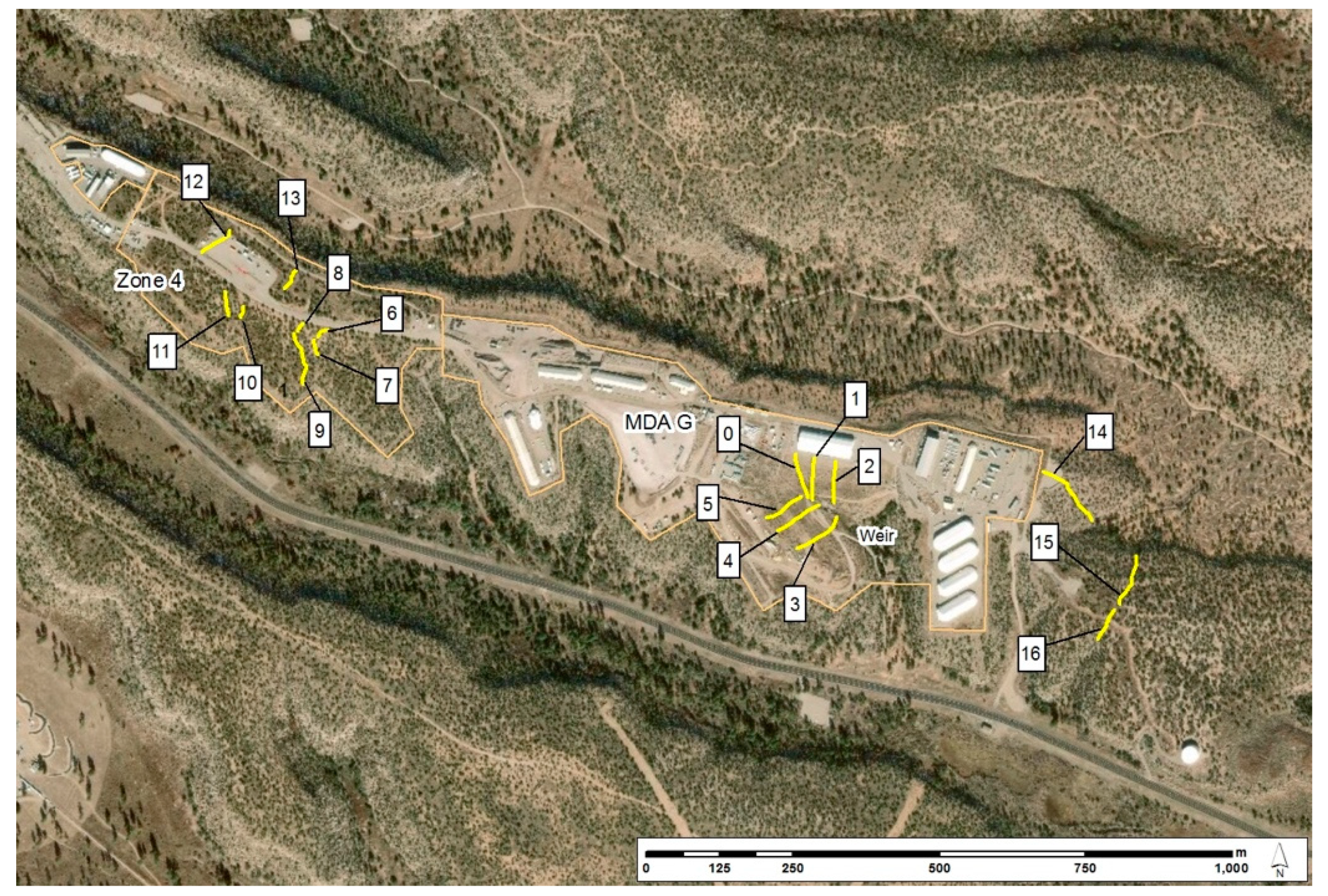
 [Green Version]
Figure 1. Location of Material Disposal Area (MDA) G with respect to the laboratory and surrounding communities.
Geosciences 09 00120 g001
Figure 2. MDA G erosion model framework.
Geosciences 09 00120 g002
Figure 3. Locations of hillslope profiles.
Geosciences 09 00120 g003
Figure 4. Initial domain shape and elevation (m) of the MDA G final cover and surrounding topography (a). Initial (after closure) estimated thickness (m) of non-native material above bedrock (b). The thickness accounts for the engineered cover and fill outside of pits but within the riprap armor. Clean fill within pits is not included in the estimated thickness. Bedrock elevation with waste pits etched in, used for SIBERIA calculations (c). Riprap armor (red) placed around the MDA G waste repository site (d).
Geosciences 09 00120 g004
Figure 5. Change in elevation (m) maps for low-, moderate-, and high-erosion cases. The top row shows results for the 1000-year compliance period. The bottom row shows results at 10,000 years, 9000 years beyond the compliance period. Below the 10,000-year planar view are cross-sectional views along the dotted black transect. Change in elevation via erosion or sedimentation overlays the bedrock with the storage pits etched in.
Geosciences 09 00120 g005
Figure 6. Change in surface elevation (m) after 10,000 years of erosion with pit locations shown for the low-erosion (a) and high-erosion (b) cases.
Geosciences 09 00120 g006
Figure 7. Thickness of engineered cover and fill material remaining above bedrock after the 10,000-year simulation period, clipped by the riprap armor layer around the mesa top for the (a) low-erosion and (b) high-erosion scenarios.
Geosciences 09 00120 g007
Figure 8. Placement of riprap armor is shown in the bottom figure; changes in surface elevation (m) for the moderate- and high-erosion scenarios are shown in the top two figures. The model predicts a ring of unchanged elevation where the riprap is present around the mesa edge.
Geosciences 09 00120 g008
Figure 9. Locations of high sediment deposition.
Geosciences 09 00120 g009
Table 1. Hillslope profile characteristics.
Profile No.Profile NameTotal Slope Length (m)SegmentsAverage Cover (%)
NumberAverage Slope (%) aCanopyGround
0Area G-1781011.26123
1Area G-274511.96424
2Area G-372613.06322
3Area G-491.5108.22033
4Area G-585.51010.02446
5Area G-672.41110.62641
6EX-1N30.545.0827
7EX-1S2744.12.97.9
8EX-2N18.349.11544
9EX-3S113.5155.52640
10EX-4S2246.21232
11EX-5S43.556.46.917
12EX-6N66.566.23261
13EX-7N40710.52757
14East-1E1381012.22972
15East-2N94.5911.02969
16East-2S7477.41854
a Segment slopes were weighted by the horizontal length of each segment to calculate the average profile slope; horizontal lengths were calculated using the slope angle and segment length.
Table 2. Runoff projections for the hillslope profiles.
ProfileAverage Cover (%)Estimated Runoff from 6-h Storm (mm/storm)
2-year Return Period5-year Return Period
NoNameCanopyGroundSandy LoamLoamSandy LoamLoam
0Area G-161231.154.810.2
1Area G-264240.84.74.39.7
2Area G-36322154.610
3Area G-420333.47.68.314
4Area G-524462.26.46.812.3
5Area G-626412.46.6712.6
6EX-1N82759.310.115.7
7EX-1S2.97.96.711.112.817.5
8EX-2N154437.27.913.5
9EX-3S26402.46.77.112.7
10EX-4S12324.38.59.214.9
11EX-5S6.9175.810.111.416.5
12EX-6N32610.824.74.39.7
13EX-7N27571.45.45.410.8
14East-1E29720.464.23.69.1
15East-2N29690.584.43.89.3
16East-2S18542.26.46.712.2
Mean27392.66.7712.4
Standard Deviation19191.92.12.72.6
Table 3. Characteristics of erosion scenarios implemented in the Infiltration and Runoff Simulation (IRS) and Hillslope Erosion Model (HEM), and the corresponding calibrated SIBERIA input parameters for the low-, moderate-, and high-erosion scenarios.
Model ParametersLowModerateHigh
Hillslope Erosion Parameters for IRS and HEM
Soil TextureSandy LoamSandy LoamLoam
Canopy Cover/Ground Cover (%)70/7030/7030/30
Landscape-Forming Return Interval (year)255
Excess Runoff (mm)2.671.2
SIBERIA Model Parameters
B = Grid Cell Runoff-driven Erosion (-)9.4 × 10−64.2 × 10−56.8 × 10⁻⁴
m = Area Sediment Yield Parameter (-)1.61.61.3
n = Slope Sediment Yield Parameter (-)0.860.870.86
Dz = Diffusion Coefficient (kg/m)0.0030.00250.005

