1. Introduction
The prediction of archaeological sites using predictive modeling is an important tool that facilitates planning for cultural resource management and the creation and testing of models of human locational behavior [
1] (p. 1). These models are classified as either inductive or deductive [
2] (p. 225). “Inductive” in this context refers to the use of a model that is based on the relationship between known archaeological sites and other attributes, as determined by machine learning methods, to predict locations of equal suitability. However, this widespread approach (as used in [
3,
4,
5,
6]) only describes first-order effects and is based on the premise that the sites are representative of the actual distribution. This is especially problematic for locations with sparse findings [
7] (p. 17). In the less frequently used deductive approach, archaeological and anthropological knowledge is modeled in order to compare the locations predicted by this model with the known find spots [
2] (p. 225). The authors in [
8] (p. 70) described such an approach with their “Cognitive predictive model”. Several examples of techniques for this approach, including the application of fuzzy logic, were provided by [
9] (p. 69). In the archaeological context, this method is used, on the one hand, for landscape reconstruction (as used by [
10,
11]) and, on the other hand, for modeling settlement preferences (as used by [
12,
13,
14]). Nevertheless, many of these approaches do not specifically address second-order spatial effects, that is, the interaction of locations with each other, as examined in [
15]. These effects are more likely to be considered in the description and analysis of existing finds [
16] (p. 314) rather than in predictive modeling.
This paper aims to evaluate whether hypotheses about spatial behavior in the Final Palaeolithic period can be spatially mapped by utilizing heuristic modeling tools and whether they can be used as a basis for distributions that represent first- and second-order effects of activity traces.
3. Materials and Methods
3.1. Archaeological Data and Hypotheses
Data on prehistoric activity from different epochs are available for the study area. In this study, we focused on the human reoccupation that occurred during the Late Weichselian. This Final Palaeolithic material is mainly distinguished by characteristic lithic artifacts attributed to the classic Hamburgian, Havelte Group, Federmesser-Groups, Brommean, and Ahrensburgian. The material of the Hamburgian and Havelte Group reflects the first recolonization of northern Germany by hunter–gatherers after the last glacial maximum, and it dates approximately to the period of the early amelioration of the Weichselian Lateglacial (cf. Greenland Interstadial 1e/d; ca. 12,690–11,970 years cal. BCE) [
20]. These pioneer populations were mainly hunting reindeer in an open tundra landscape with some shrubs and first trees in river floodplains [
21,
22]. In total, the material from the Hamburgian was found in 20 find spots, of which 7 could be further attributed to the classic Hamburgian, and 6 could be ascribed to the Havelte Group. The material of the Federmesser-Groups, as well as the Brommean, is associated with light forest environments during the second part of the Weichselian Lateglacial (cf. Greenland Interstadial 1c–a; c. 11,970–10,770 years cal. BCE) [
22,
23]. The preferred prey animals in this period were elks that roamed in the widespread lake and pond landscapes of this period [
23,
24]. In 81 locations, material from these elk-hunting communities was found. Material of only the Federmesser-Groups was found at 27 of these sites, and indicators of only the Brommean came from 44 find spots. The Ahrensburgian material dates mostly to the Younger Dryas (cf. Greenland Stadial 1; 10,770–9,670 years cal. BCE) [
25], during which a park tundra landscape spread, and reindeer became the main prey animal for hunter–gatherers [
22,
26]. A total of 37 sites were attributed to this archaeological group. Since the total number of sites from each period is rather small, and we assume that the hunting economy had an impact on the settlement system [
27,
28], we combined the Federmesser-Groups and Brommean elk-hunting groups into one set and the clearly chronologically distinct reindeer hunters of the Hamburgian and the Ahrensburgian to another set. Although these groups had to face different obstacles and, therefore, developed different mobility strategies, our hypotheses are so generalized at this stage that they apply similarly to groups in similar habitats.
The artifacts used for comparison were recovered as single finds, small and large collections, and systematic surveys or excavations that had been reported to the Archaeological State Office Schleswig-Holstein. These reports formed the archaeological atlas from which the data of the sites were retrieved. Testing the distribution of sites against the activities of collectors indicates that there is no direct correlation detectable but well known areas such as the Ahrensburg tunnel valley attract more activity in general. Furthermore, depending on the circumstances (e.g., time of collection, knowledge of the collector/excavator’s previous work), some flint concentrations were considered as a single site, whereas, in other cases, several concentrations were attributed to the same site. If these originated from different archaeological periods, then they were differentiated. However, this practice can result in an accumulation of data points in some areas, whereas other areas in which just as much material was concentrated are assigned only one data point. Therefore, single finds have been removed before the modelling process and finds of the same time with a distance of less than 1000 m between each other were combined to counteract this problem. A further weighting of differently large numbers of finds did not take place.
The preferred spaces of elk hunters and reindeer hunters were reflected by forming the hypotheses on the basis of finds and assumptions, which are used for spatial modeling. For reindeer hunters, it is assumed that the accessibility of flintstone was important and that their settlement follows reindeer migration routes and, therefore, lies predominantly in water-rich valleys [
29]. For elk hunters, on the other hand, the hypothesis is that they settled on low, dry, and sandy ridges in the vicinity of waters and, similar to the reindeer hunters, close to local flint occurrences [
30,
31].
3.2. Geomorphometric Data
Hypothesis-driven prediction requires data sets that allow for a spatially explicit representation of these hypotheses. A digital elevation model with a cell size of 25 × 25 m [
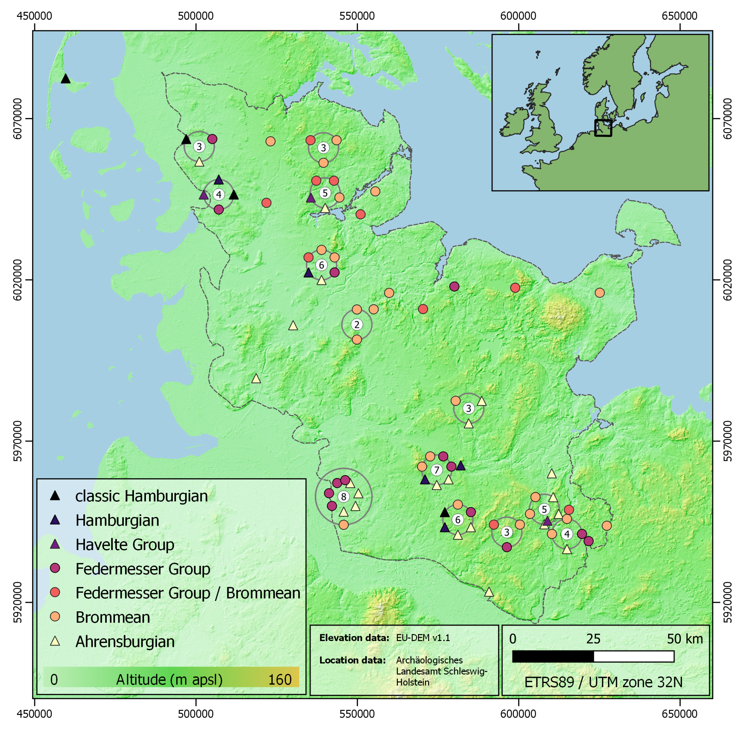
32] served as the base of the modeling process, and it covers the entire study area of Schleswig-Holstein (
Figure 1). Only the natural unit of the marsh was removed from the elevation model using the major natural units according to Meynen and Schmithüsen [
33]. This decision was made because the marshes developed after the period relevant to this paper, and applying the model approach to the elevation model of these areas and the parameters derived from it would otherwise be problematic. We are also aware that the other units were altered by post-depositional processes (e.g., plow zone destruction, outwash, and deposition by colluvia or coversands), but, in total, these areas were not affected as comprehensively as the marshes. The amount of data that would be necessary to reconstruct the palaeolandscape on a state-wide scale for the approximately three different Final Palaeolithic periods cannot be reliably reviewed and processed with the available means. Hence, we are aware that using modern elevation models adds additional biases of preservation conditions and the accessibility of the archaeological material. The reduced elevation model was used to calculate the geomorphometry of the study area. This includes parameters that were generated using GRASS GIS [
34]:
Topographic index represents the gravitational forces that move water—which tends to gather at any point in the catchment—downslope [
35]. The index is used to detect potentially wet areas using today’s relief.
Geomorphons constitute a nominal parameter that shows different landforms, such as ridges and valleys [
36].
Additional parameters were also generated to determine the position in the relief using SAGA GIS [
37]:
Positive openness is a metric parameter that indicates the degree of openness of the area surrounding a location. Low values represent higher elevations in the surrounding area. High values indicate the lack of higher elevations around the location [
38].
Negative openness is similar to positive openness but is focused on the lowest points. A low score of negative openness means that the lowest points in the area surrounding a location are lower than those in the location, while a high score indicates that the lowest points are higher than those in the location [
38].
Furthermore, the Geological General Map of the Federal Republic of Germany [
39] was used to express the dependence on the raw material flint, and the Soil Map of Germany [
40] was used to identify water bodies and moorlands as potential palaeo-water bodies.
3.3. Fuzzification
The first step in the modeling process (Complete R-Code in the
Supplementary Materials) was the conversion of the hypotheses into spatially explicit grids. The hypotheses were expressed using the heuristic modeling tool FuzzyLandscapes [
41] and the geomorphometric grids mentioned above. The fuzzification is based on the theory of [
42]. According to the theory, a linguistic hypothesis, such as
Flint was available nearby, is expressed by assigning a function to a metric variable that assigns a membership degree between 0 and 1 to each value of the metric variable. The metric variable in this case is the distance to moraine areas (calculated by the function
r.grow.distance [
34] using the Geological General Map [
39]) because these areas are considered to be secondary deposits for flint [
43] (p. 85). As
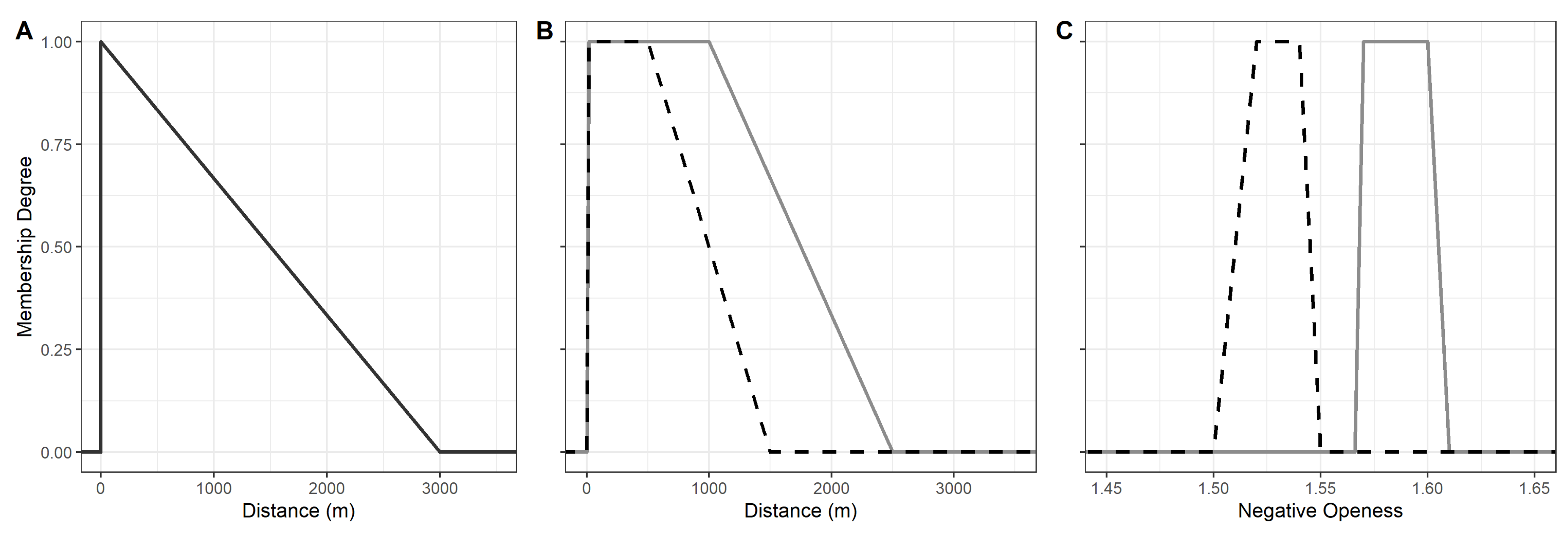
Figure 2A shows, a function assigns a membership degree between 0 and 1 to each distance. This function was applied to the raster data set using the FuzzyLandscape package [
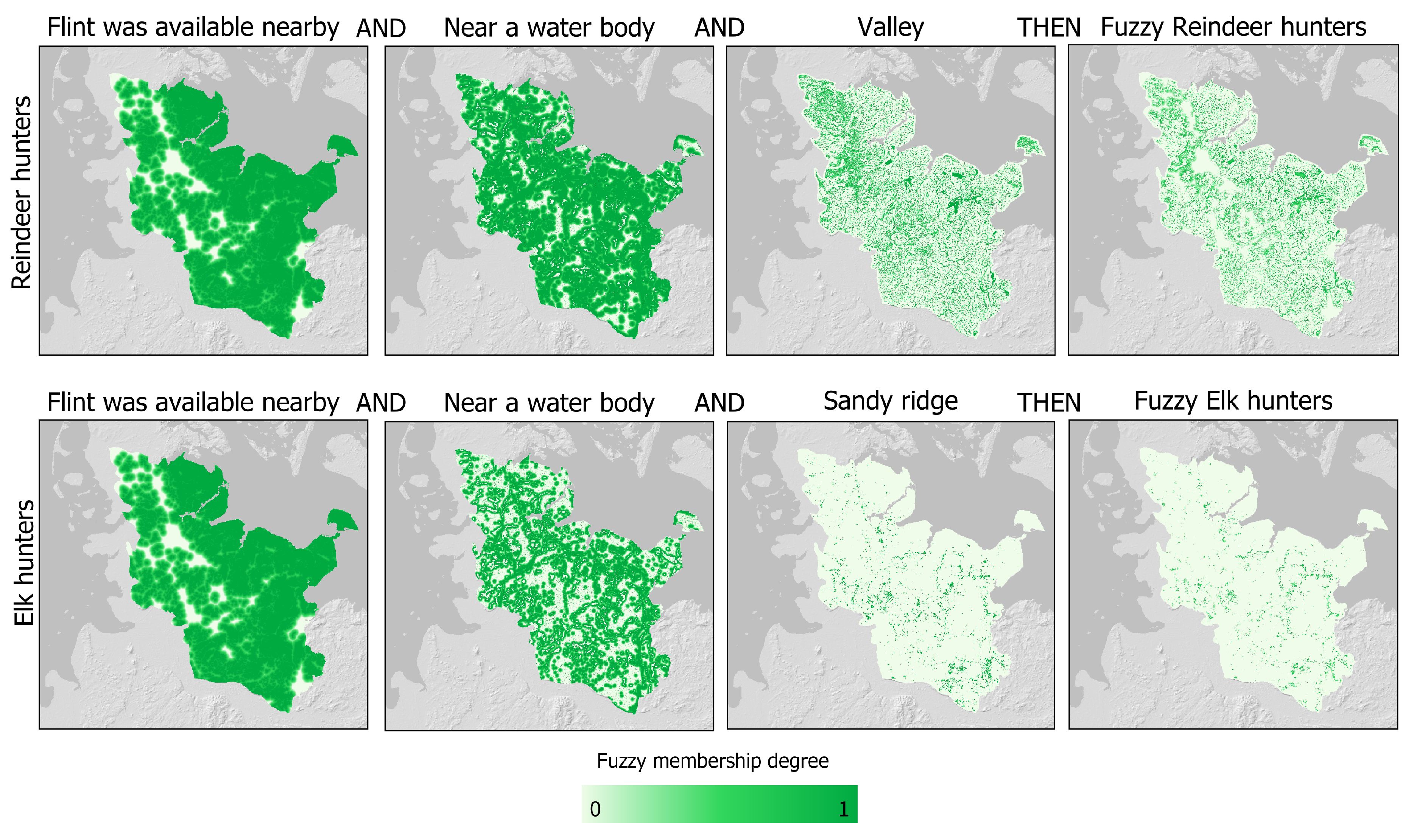
41]. Accordingly, each raster cell was assigned a value corresponding to the membership degree of the fuzzy set (
Figure 3, left). In addition to the linear functions (
Figure 2), the FuzzyLandscapes package [
41] also provides nonlinear fuzzifications. The linear functions—as the simplest approach—were chosen because there are no further hypotheses about the attractiveness of the resources, which could be implemented in a more complex nonlinear function.
Since flint is elementary to the hypotheses stated above for both elk hunters and reindeer hunters, the fuzzy set was used for both groups. Furthermore, the bases of the fuzzy set
Near a water body are the same data sets. These are the topographic index, the distance to moorlands, and the distance to today’s water bodies. However, since reindeer hunters in the dominant open tundra had fewer obstacles than elk hunters in light forests, farther distances were considered acceptable to apply to the reindeer hunters, which is reflected in the fuzzification of the data sets (
Figure 2B).
These fuzzified data sets were then combined to create the fuzzy set
Near a water body (
Figure 3). Following [
42], for each cell, the membership degree was obtained, which had the highest value of the three combined grids: this is linguistically expressed as “
The cell is close to a mire OR
the cell is close to a recent water body”. This is referred to as “union” in set theory [
44] (p. 340). The resulting data set
Near a water body is connected to the
Flint available nearby fuzzy set by an intersection [
44] (p. 341), which means that the minimum value is assumed for each raster cell. This is expressed as AND in linguistic terms.
The fuzzy set
enclosed was derived from the calculated negative openness [
38] and unioned with the set
low openness, which was derived from the calculated positive openness, and the crisp (in this case, binary) valley factor (the function
r.geomorphon [
34]) in order to reflect the preferred occupancy of valleys by reindeer hunters. Since the hypothesis states that elk hunters preferred sandy ridges, negative openness was also used for this group; however, the function is defined in such a way that it determines a ridge and not a valley (
Figure 2C). The positive openness was not used because a ridge can be located in a large valley as well as a plain. Instead, the Pleistocene fluvial sand areas, which were derived from the Soil Map of Germany [
40], were introduced as crisp variables and intersected with the ridge fuzzy set. The previous steps resulted in two raster data sets that contained the membership degree for the hypothesis of the distribution of reindeer hunters and elk hunters (
Figure 3, right).
3.4. Point Distribution
The second step was the simulated placement of potential settlement traces—with consideration given to higher preferences—in areas with high suitability (e.g., with a high fuzzy membership degree). Two different approaches to determining the distribution were applied. The first approach is a random Poisson distribution applied by the function
rpoispp, as described by [
45]. The intensity of the Poisson process is thereby represented by the membership degrees of the fuzzy set raster. The location of the points is solely dependent on the probabilities defined by the input grids. However, the points do not influence each other. Therefore, according to [
46] (p. 259), the first approach represents only first-order properties. The second approach uses the same random Poisson distribution, but, in addition, creates random clusters around the Poisson points using the function
rPoissonCluster [
45]. For this function, four locations within a radius of 2000 m were selected by using empirical comparisons with the data of the Archaeological State Office Schleswig-Holstein. In doing so, spatial dependence was integrated into the simulated spatial point process. Therefore, the potential settlement traces are represented by not only first- but also second-order properties [
46] (p. 259).
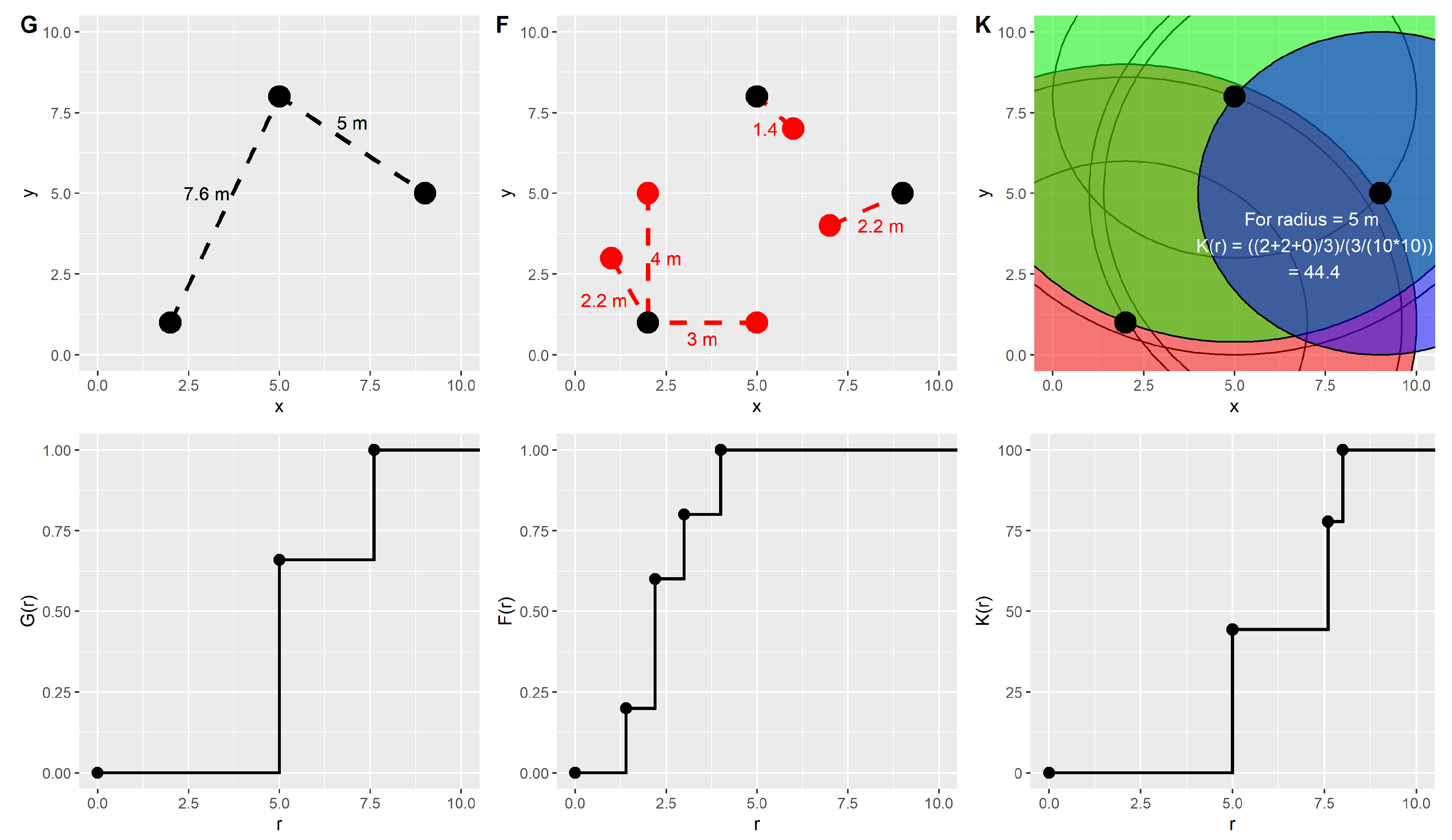
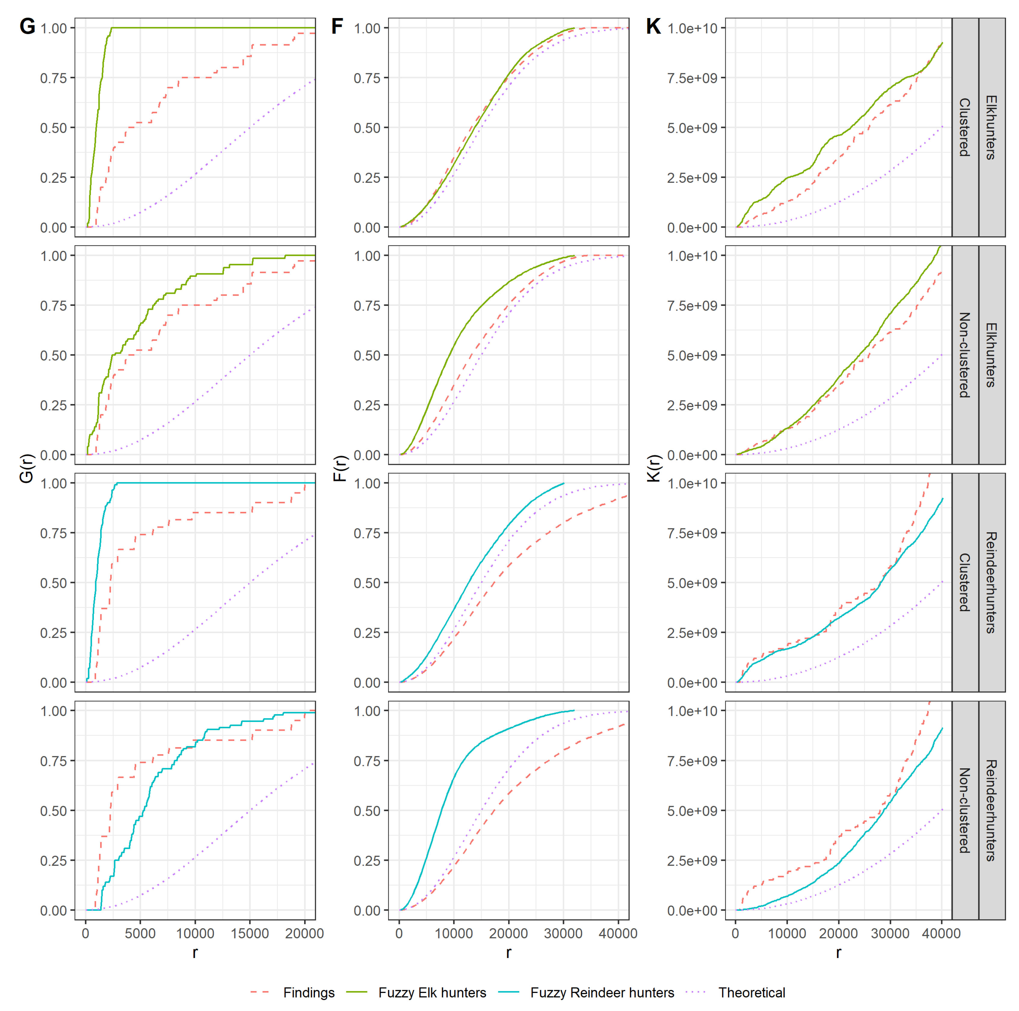
Three functions—G, F, and K—were used to compare the simulated points based on the hypotheses with the actual find spots regarding effects of the first and second order [
15] (p. 9). First, the nearest-neighbor distance distribution function (
G(
r), following [
45] (p. 262)), was used. The method is illustrated in the left part of
Figure 4. For each examined point, the distance (
r) to the nearest neighbouring point is calculated (top left). As described by [
45] (p. 285), the proportion of points with a shortest distance to the nearest neighbor smaller than
r (
G(
r)) is then juxtaposed with the respective
r (bottom left). In the example at a distance (
r) of 5 m, two of three points are connected to their nearest neighbour resulting in an
G(
r) of 0.67. In addition, the empty-space function (
F(
r), following [
45] (p. 262)), was applied to the observed and modeled point patterns. This function is similar to the
G(
r) function, but, instead of the cumulative distances of known points, the distances from randomly generated reference locations to the nearest data points are observed. This is illustrated in the example (
Figure 4 centre) by randomly distributed locations (red) of which the distance to the nearest observed neighbour (black) is calculated. The third tool that was applied to the point distributions is Ripley’s K function (
K(
r)) [
47], a common tool used for spatial descriptive statistics. As illustrated in
Figure 4 (right), the empirical K-function calculates the average number of data points lying within a radius
r of the data points [
45] (p. 204). Unlike the F- and G-function, the K-value is standardized by dividing the number of points by the intensity; that is, the total number of points is divided by the area extended by the locations of all points [
48] (p. 64), which results in much larger values (
Figure 4).
Each of the three functions illuminates different aspects of spatial relationships. With the G(r) function, the focus is only on the nearest neighbour of the locations. If each point has only one close neighbour, this is represented by a steeply rising curve. The more locations are further away from the closest neighbour, the flatter the resulting curve will be. The F(r) function, on the other hand, shows the general tendency towards cluster formation. If many points are clustered, the randomly distributed reference locations map the larger free areas by further distances. A larger r is required until a larger proportion of the reference points have their nearest neighbour, which leads to a flatter curve. The steepest increase of the F(r) function is reached with a regular point distribution because, in this case, every randomly distributed point has a very close neighbour. Since the K(r) function, in contrast to the other functions mentioned above, represents not only the nearest but all neighbours, it is particularly suitable for mapping the size of the clusters and the distance between them. The first rise of the curve to the first flattening shows the average distance (r) of nearby points surrounded by empty space. Every next increase indicates the distance to the next clusters.
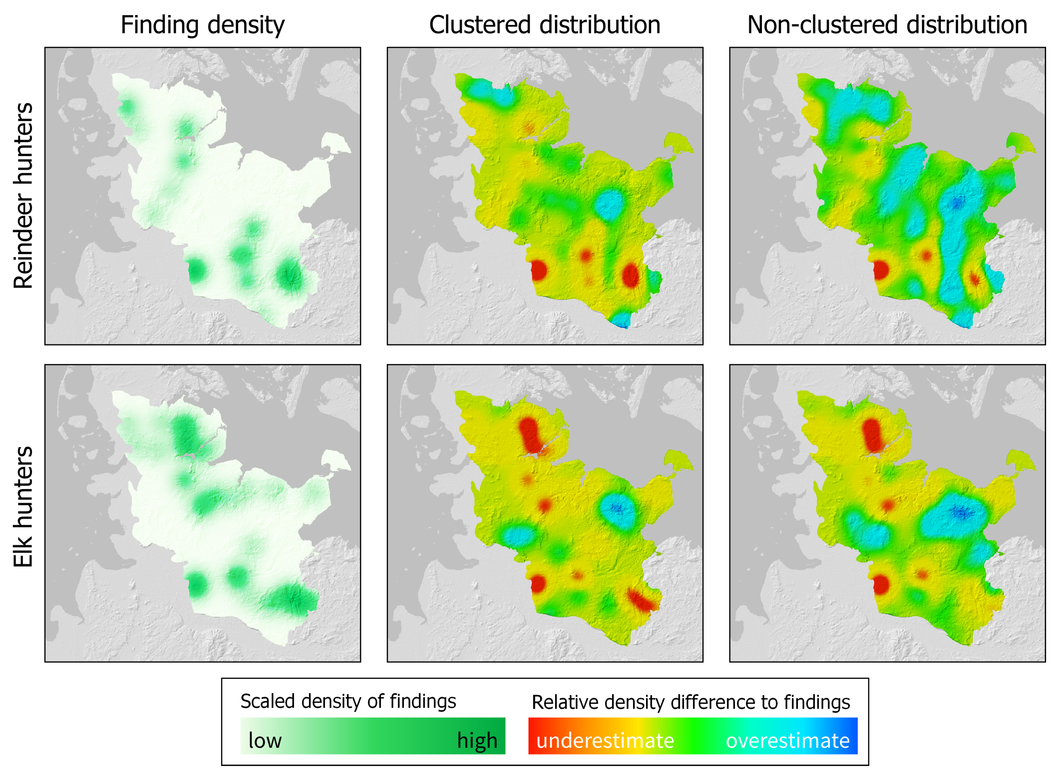
In addition to the functions representing the relative locations of the modeled points and the find spots, a kernel density estimation is applied to the point patterns (function
density.ppp of the spatstat library). An isotropic Gaussian density function was selected with a bandwidth of 6134 m for this kernel estimation. Thereby, the bandwidth resulted from the application of the function
bw.ppl, which itself uses a likelihood cross-validation method to select a smoothing bandwidth for the kernel estimation [
45] (p. 171). The resulting grids were normalized by the value ranges and subtracted from the normalized density of the find data.
4. Results
Figure 5 shows the results, separated by elk hunters and reindeer hunters, of applying the F-, G-, and K-functions to the random and clustered point distributions and the actual find spots. They also contain a dotted
Theoretical line that represents a completely random point pattern. As mentioned above, the empty-space function
F(
r) displays the probability of detecting a point within the radius
r of an arbitrary reference location [
45] (p. 262). For the elk hunters, this function does not distinguish between the actual locations and a completely random point pattern. The points distributed in clusters according to the fuzzified hypotheses also reflect this. For reindeer hunters, the line of actual sites falls short of the theoretical distribution, indicating a clustered point pattern [
45] (p. 266). As with the non-clustered distributed points of the elk hunters, the spreads of the points according to the fuzzified hypotheses for reindeer hunters indicate a regular point distribution.
The nearest-neighbor distance distribution function (
G(
r)) reveals clustered distributions for all hypothesis-based distributions and the find spots [
45] (p. 267). As expected, the clustered points show much stronger signs of clustering because several points were distributed at each location selected on the basis of the fuzzy grids. For the actual finds, the individual points are farther from the nearest neighbor; this is not possible with the clustered distributed points. The non-clustered distributed points for the elk hunters approach the distribution of the actual finds, while, for the reindeer hunters, especially in the area up to about 7000 m, the clustering of the actual finds is much stronger. The interpretation of the variations in
K(
r) is the inverse of that in the
F(
r)-function [
45] (p. 266). Instead of showing the size of the empty areas, the extent of the increasing radii is shown. The figures show that the data found and modeled deviate considerably from the theoretical random Poisson distribution.
Figure 5 (K) also reflects the results indicated in the previous plots. For the elk hunters, the clustered distributed points overestimate the actual clustering of the finds, while the non-clustered distributed points have a higher correspondence to the distribution of the actual finds. The clustered distribution of the reindeer hunters, on the other hand, is more likely to reflect the actual find situation than the non-clustered distributed points, especially for short distances. Comparing the results of the
G(
r),
F(
r) and
K(
r) functions, it is noticeable that, for elk hunters, the
G(
r) and
K(
r) functions indicate clustering, while the
F(
r) function indicates a random or regular pattern. This seemingly contradiction suggests that there are many small clusters of elk hunters which are relatively randomly distributed throughout the whole area. Thus, the
G(
r) and
K(
r) functions emanating from the sites show clusters while the
F(
r) functions emanating from the empty space show randomness and a tendency to regular arrangement.
In addition to the relative positions of the points to each other, the absolute position in space is also important (left of
Figure 6). The densities of the actual finds differ between the elk hunters and reindeer hunters. Especially in the northern part of the study area, the find densities for elk hunters are higher than those for reindeer hunters. In the locations of the elk hunters, both the clustered distribution and the non-clustered distribution are observed to have considerably lower point densities at the actual sites. The non-clustered distribution is closer to the actual point density only in the southeast. However, although the positive deviations resulting from both methods tend to be higher in the areas with lower find densities, they are smaller in the clustered distribution and thus better correspond to the find situation. This trend toward greater overestimation in the areas of low find density by the non-clustered distribution is even more evident among reindeer hunters (as indicated by the large blue areas in
Figure 6).
5. Discussion
In this study, we investigated whether hypotheses about spatial behavior can be spatially explicitly mapped with heuristic modeling tools and whether these can be used as a basis for distributions for first-order and second-order effects. Both points must be affirmed. With the functionality of the FuzzyLandscapes [
41] package, it is possible to map spatially explicit hypothesis-based areas that are in high and low agreement with these hypotheses. A comparison of the results achieved in this study with those reported by other authors remains difficult. We deliberately decided against using a machine learning method, such as Genetic Algorithm for Rule Set Production (GARP), as used by [
49], or multiple linear regression, as applied by [
13], to determine the relationship between the variables available on a large scale and the settlements in order to incorporate the knowledge generated in this way into the hypotheses. This procedure poses the risk of merely predicting locations at which sampling is preferred. This risk always exists if the finds do not represent the population of the settlement traces, which is the case for archaeological examinations of an area with the size of the study area.
In our case study—the elk hunters and reindeer hunters—the approach presented here clearly demonstrates that, for the reindeer hunters, a mapping approach that only includes spatial effects of the first order cannot completely reflect the characteristics of archaeological settlement traces. The clear difference between clustered and non-clustered distributed points is especially apparent with Ripley’s K-function (
Figure 5), which is used to describe second-order spatial processes. It should be noted that this second order effect does not necessarily reflect a contemporaneity of points. Ultimately, the locations of humans with the same location requirements, such as the reindeer hunters, but, from different phases—i.e., the Hamburgian and the Havelte Group as well as the Ahrensburgian (which themselves represent large periods of time)—were compared. Rather, second order effects here represent the spatial memory of groups of equal demands, which is expressed by the repeated use of the same or a nearby location. Accordingly, we do not assume an influence of the find spots on each other but rather an influence of the memory of temporal occupation (represented by finds) on find spots. Meanwhile, we do not assume that the available resources alone determined the choice of location, which would be the definition of a first order effect. Rather, good conditions were also present in the northeast as illustrated by the non-clustered distribution (
Figure 6, top right), but these good conditions were either not used by the reindeer hunters or not preserved (top left). Thereby, the find spots of the elk hunters (
Figure 1) in these areas show that the lack of reindeer hunter finds was not caused by a lack of archaeological sampling. In the case of elk hunters, though, there is a greater similarity between the non-clustered points and the finds. However, an examination of the differences in point density (
Figure 6) shows that neither the clustered nor the non-clustered points fully capture the high point densities of the actual finds, especially in the north of the study area. This indicates that the hypotheses do not reflect the circumstances that led to the settlement in the north.
For elk hunters, the combination of sandy subsoil and the proximity to flint occurrences results in low membership degrees in this area. In the areas of lower find density in the east, the clustered points have a more suitable point density, which leads to the conclusion that consideration of second-order effects enhances the spatial prediction. It should also be noted that a high point density or a cluster of points do not necessarily represent settlements from the same phase. A high point density is also an expression of spatial memory by cultures that behave similarly because they share similar circumstances. Elk hunters in this context are not a uniform culture; they represent two different archaeological units for which similar hypothesis-based spatial demands are assumed (
Figure 2). Reindeer hunters have a stronger clustering than elk hunters, which can also be illustrated by the comparison with the simulation (
Figure 5). When examining the reindeer hunters, the Ripley’s K-plot of the actual finds shows a cluster size of about 2–3 km. The recurring settlements varied around this radius. In addition, an increase of about 17 km shows the cluster separation—the distance between the clusters. This indicates that reindeer hunters often returned to the same places, but, because of the open tundra landscape, the exact location could be varied more easily than the locations selected by elk hunters in the light forest landscape, in which the cluster size and separation are not visible.
Figure 3 supports this assumption by showing that the areas suitable for elk hunters are more thinly distributed than the areas that we suggested as suitable for reindeer hunters.
The different correspondences between our hypotheses and the actual sites of elk hunters and reindeer hunters—and hence their verifiable settlement behavior—were mainly because the (large mammal) hunting economies could lead to different considerations. One possible explanation for this might be greater uniformity of the landscape during the colder periods and a great diversity during the warmer Allerød period. However, according to the results of an ongoing Ph.D. project on the vegetation development during the Late Weichselian [
50] the allocation of the study area to a northern and southern as well as a western and eastern environmental sector began quite early in the Lateglacial and would have affected the environments of all analyzed periods. However, if we compare our findings with the explanations given for the early colonization of North America [
28], we could assume (with all due respect to the scarcity of our record) that the elk hunters and the reindeer hunters depended on large mammal hunting and local resource microstructures to different degrees. Since the settlement behavior of the reindeer hunters seems to be better reflected, these mobile groups could have been mainly dependent on their hunting economy, allowing them to disregard the local resource microstructure and to return to good hunting spots of their predictable prey. In contrast, the settlements of the elk hunters appear not as well reflected by these hypotheses, suggesting a greater dependence on the local distribution of resources and greater independence of large, less predictable mammal hunting (cf. [
28]). For our approach, this would mean that, in particular, to understand and predict the behavior of elk hunters, we would need to reconstruct their environments in greater detail, take different prey ethology into account and consider the influence of other resources on their settlement strategies.
Future work could look at the ability to successfully downscale this approach. This would result in more detailed fuzzy grids and thus more detailed representations of the hypotheses, as well as greater certainty as to whether settlement traces in an area were not present or just no longer locatable. After all, in the area of fuzzification, there are currently still limits to the approach. The elevation model and the other data sets on which it is based represent current conditions. For example, if we assume that today’s mires were Palaeolithic water bodies, a more detailed consideration of a smaller area, perhaps even a reconstruction of the elevation model, could lead to more realistic simulations. Furthermore, because marsh areas arose only after the considered time, their rough extinction could be reconsidered with a reconstructed elevation model, possibly also including the landscapes of the North Sea Basin that are submerged today but were accessible during the Late Weichselian (cf. [
51]). In addition, the behavior that is shown in
Figure 5 (G) could be modified during cluster formation so that, in addition to the distribution of the points that follow a Poisson distribution, the number of points per cluster is randomized. Of course, it would also be interesting to determine whether the underestimated areas of the elk hunters in the north could be mapped more accurately by adjusting the hypotheses, adding more information (such as soil or vegetation development), or both (cf. [
52]). In future studies, besides the further adaptation of the hypotheses for the elk hunters in northern Germany, the application of this approach in other areas and for other cultures would be beneficial.
