Article

Insights into the Short-Term Tidal Variability of Multibeam Backscatter from Field Experiments on Different Seafloor Types

1
Royal Belgian Institute of Natural Sciences, Operational Directorate of Nature, Gulledelle 100, B, 1200 Brussels, Belgium
2
Department of Geology, Renard Centre of Marine Geology, Ghent University, Krijgslaan 281 s.8, B-9000 Gent, Belgium
3
Federal Public Service Economies, Continental Shelf Service, Boulevard du Roi Albert II, 16, 1000 Brussels, Belgium
4
Ifremer, Underwater Acoustics Laboratory, IMN/NSE/AS, CS 10070, 29280 Plouzané, France
*
Author to whom correspondence should be addressed.
Geosciences 2019, 9(1), 34; https://doi.org/10.3390/geosciences9010034
Submission received: 4 December 2018 / Revised: 24 December 2018 / Accepted: 2 January 2019 / Published: 10 January 2019
(This article belongs to the Special Issue Geological Seafloor Mapping)

Abstract

:
Three experiments were conducted in the Belgian part of the North Sea to investigate short-term variation in seafloor backscatter strength (BS) obtained with multibeam echosounders (MBES). Measurements were acquired on predominantly gravelly (offshore) and sandy and muddy (nearshore) areas. Kongsberg EM3002 and EM2040 dual MBES were used to carry out repeated 300-kHz backscatter measurements over tidal cycles (~13 h). Measurements were analysed in complement to an array of ground-truth variables on sediment and current nature and dynamics. Seafloor and water-column sampling was used, as well as benthic landers equipped with different oceanographic sensors. Both angular response (AR) and mosaicked BS were derived. Results point at the high stability of the seafloor BS in the gravelly area (<0.5 dB variability at 45° incidence) and significant variability in the sandy and muddy areas with envelopes of variability >2 dB and 4 dB at 45° respectively. The high-frequency backscatter sensitivity and short-term variability are interpreted and discussed in the light of the available ground-truth data for the three experiments. The envelopes of variability differed considerably between areas and were driven either by external sources (not related to the seafloor sediment), or by intrinsic seafloor properties (typically for dynamic nearshore areas) or by a combination of both. More specifically, within the gravelly areas with a clear water mass, seafloor BS measurements where unambiguous and related directly to the water-sediment interface. Within the sandy nearshore area, the BS was shown to be strongly affected by roughness polarization processes, particularly due to along- and cross-shore current dynamics, which were responsible for the geometric reorganization of the morpho-sedimentary features. In the muddy nearshore area, the BS fluctuation was jointly driven by high-concentrated mud suspension dynamics, together with surficial substrate changes, as well as by water turbidity, increasing the transmission losses. Altogether, this shows that end-users and surveyors need to consider the complexity of the environment since its dynamics may have severe repercussions on the interpretation of BS maps and change-detection applications. Furthermore, the experimental observations revealed the sensitivity of high-frequency BS values to an array of specific configurations of the natural water-sediment interface which are of interest for monitoring applications elsewhere. This encourages the routine acquisition of different and concurrent environmental data together with MBES survey data. In view of promising advances in MBES absolute calibration allowing more straightforward data comparison, further investigations of the drivers of BS variability and sensitivity are required.

1. Introduction

The North Sea is amongst the most highly impacted areas of the marine biome [1]. This is particularly the case for its Belgian part, where a multitude of anthropogenic activities, including intense routed navigation, dredging and disposal of dredged material, marine aggregate extraction, bottom trawling by commercial fisheries and extensive infrastructural, engineering and management developments (e.g., telecommunication cables, pipelines, wind energy and beach nourishment), take place over a limited spatial extent of ~3600 km2 along a ~65 km coastline [2]. In this regard, knowledge of the seafloor composition and of its spatio-temporal evolution is of great relevance to monitor human impacts on benthic habitats (of which substrate type is a fundamental abiotic component and surrogate for biota [3]). At the European level, the monitoring is mandated by the European Marine Strategy Framework Directive to achieve Good Environmental Status (GES) of marine waters by 2020 (see [4] and references therein). Twelve GES descriptors were put forward for which each EU Member State defined indicators with associated monitoring programmes. For the Belgian part of the North Sea (BPNS), one of them relates to changes in the extent of seabed habitats for which multibeam echosounding (MBES) was selected for the monitoring [5].
The use of MBES systems to acoustically characterize the seafloor has developed at a fast pace over the past three decades [6,7]. Co-registration of depth (signal travel-time) and reflectivity (backscattered intensity of the echo signals, hereafter BS) measured over a large range of angles (swathe) and at very high resolution is possible using this technology. MBES BS depends on many factors, including ([8]): (1) sediment type and its geotechnical characteristics dictating the seawater-seafloor impedance contrast (e.g., porosity, roughness, grain size and sediment inner homogeneity), (2) the sonar operating frequency, and (3) the signal angle of incidence. Due to the various sound-scattering properties of different seafloor substrates, BS can be used as a proxy aiding in the determination of bottom type at the water-sediment interface (e.g., [9,10]) and possibly the inference of some of its physical characteristics [11,12]. Mapping this interface over vast areas allows extending information from local observations (in situ ground-truth measurements) or transect-based information, that need interpolation/extrapolation [13], to the spatial continuum of the seafloor. This is valuable as an input to Marine Spatial Planning and Ecosystem Based Management and aids in the creation of efficient analytical, managerial and decision-making tools [14,15,16,17].
Backscatter data obtained from MBES surveys are usually considered at two processing levels: angular response (AR—signal processing) and mosaicked images (image-analysis). The AR describes the backscattering strength variation with angle of incidence and is retained as an intrinsic property of the seafloor directly relating to physical quantities of interest [18]. This “raw” format of backscatter is a promising seabed classification feature with a high potential for sediment discrimination, as reported in a range of studies ([19,20] and references therein). The AR forms a shape (“the AR curve”) which reflects the dominant acoustic phenomena occurring along the angular domains: high-intensity specular reflection around the nadir and lower-level scattering at oblique angles, strongly decreasing at shallow grazing angles. Where absolute calibration of the BS is achievable, the BS AR is to be considered as an objective measurement for which different methods exist ([21] and references therein). The mosaic backscatter is a further derivative of the backscatter data, where BS levels are presented, usually in a georeferenced frame, in the form of a grayscale image with the angular dependence removed via statistical compensation. As such, the complete scene seems to be observed from the same incidence angle which is generally obtained by normalizing the data and referencing it to a conventional angle or a limited range of angles. Typically, this is around 45° where the angular dependence is weakest and where the sediment response dominates [12]. Both BS data forms (AR and mosaicked images) have been used to predict seafloor type, on their own, or in combination with other MBES data types [20,22]. The main differences between these two formats are the spatial resolution and the type of information they contain. The BS AR is obtained by averaging a set of consecutive pings and processing them over the swath extent or over areas of interest, resulting in a resolution approximating that of the area selected. The BS mosaic resolution is considerably finer, given that it can be gridded as a function of the bathymetric resolution. Here, identification of small-scale features (down to decimetric orders of magnitude for high-frequency MBES operated in shallow waters) is feasible and is particularly valuable to ecological modelling requiring detailed discrimination of substrate distribution, down to the spatial-unit level of single patches [23,24,25]. However, due to its inherent compensation of angle dependency, the mosaicking process leads to a loss of quantitative/physical information, making immediate ground truthing critical for effective relation to seabed properties. On the other hand, the AR can be interpreted via modelling of the response and fitting of parameters (see [26] and references therein) which directly relate to the physical nature of the underlying substrate. Inversion of the AR into sedimentologically relevant information is a principle known for long which is currently hindered by a lack of high-frequency geoacoustic models dedicated to solving the “inversion problem” and should be perceived as an advancing application within the realm of acoustical oceanography. However, it remains promising considering the rapid advances in MBES system absolute [21,27,28] and relative calibration [29] and in stability and repeatability controls [30], together promoting the comparability of data in space and time. This would also allow compiling acoustic inventories that are calibrated against substrate types (and of associated features and combinations) to be used more globally. Alternatively, ground-truthing developments allow an increasingly detailed characterization of the acoustic observations and thus the potential development of models otherwise constrained by the need for a priori knowledge. In the long term, the scientific community would largely benefit from the development of detailed high-frequency geoacoustic models offering the advantage of directly exploiting the remotely sensed data, thus reducing labour-intensive and often expensive ground-truthing operations. Methods exploiting the AR demonstrated the utility of inverting radiometrically calibrated and geometrically corrected backscatter data into relevant sedimentological parameters [22]. However, the latter were related to well-sorted and homogeneous sediments only, evidencing the need to enhance the understanding of the relations between naturally complex sediment configurations and the retrieved acoustic signatures and to ground truth the acoustics to avoid misleading interpretation (regardless the type of BS product and approach used).
Environmental monitoring, based on the acquisition of MBES time series [31,32], requires investigating and understanding the repeatability and variability of the data. Besides the instrumental constraints (aimed at ensuring the consistency of measured data from different campaigns and/or sensors), multiple sources of environmental factors must be considered for their impact on the consistency and accuracy of backscatter data measurement. This is particularly the case in nearshore/coastal and continental shelf zones where seafloor and water-column variability may be high at diverse scales in space and time. Therefore, it is important to evaluate whether changes in the average backscatter level between different surveys reflects actual changes in sediment properties or in the conditions of the water medium [33] and of other dynamic parameters. A similar concern was already identified in terrestrial remote-sensing applications [34,35]. In this regard, it is critical that the survey-design phase of any such investigation considers all possible sources of variation which may contribute to unwanted fluctuations of the backscatter strength. This is needed to confidently quantify seafloor type and change based on the acoustic returns.
Depending on the MBES survey environment, a range of factors can be responsible for unwanted signal fluctuations in the acoustic measurements. First, the azimuthal dependence is driven by the orientation of small-scale bed forms relative to the navigation heading (hence the acoustic line of sight; see [10,36,37,38,39]), as well as by seafloor mobility under the effect of hydrodynamic forcing driving the roughness polarization. Second, the dissipative nature of the water medium leads to absorption of acoustic energy during the signal propagation; this depends on the seafloor-target range, frequency and physico-chemical properties, such as temperature and salinity driving the viscous-thermal status [40,41,42]. The concentration and particle size and shape of suspended particulate matter (SPM) also contribute to the total two-way transmission loss of the acoustic signal; it can be significant in nearshore and shelf environments (particularly over relatively long distances, i.e., typically beyond 100 m—see [43]). Finally, biological activity, occurring in the water column (e.g., the Deep Scattering Layer—see [44]) or at the benthic level (referring to epibenthic and infaunal activity—see [37,45]), as well as near-bed advection of submerged aquatic vegetation ([17]) can affect MBES measurements. Additionally, there is a need to better understand the effects of the intrinsic dynamicity of given substrates and how near-bed (also referred to as boundary and/or water-sediment interface and benthic zone) sediment transport affects the seafloor sonar detection. Ideally, all of these variables are accounted for when comparing datasets in space and time.
This study presents a set of observations originating from three experimental datasets acquired to understand and quantify the external and seafloor-intrinsic sources of variance that may lead, while surveying, to biases in the seafloor backscatter acquired by high-frequency (300 kHz) multibeam sonar systems. Repeated measurements (multi-pass MBES surveys) using EM3002D and EM2040D echosounders are interpreted based on seafloor and water-column data acquired by grab sampling, optical observations and a multi-sensor benthic lander, in combination with a drop-down frame. Altogether, these data are used to assess the sensitivity of the BS and how its short-term variability can affect the detection of actual changes in the seabed.

2. Materials and Methods

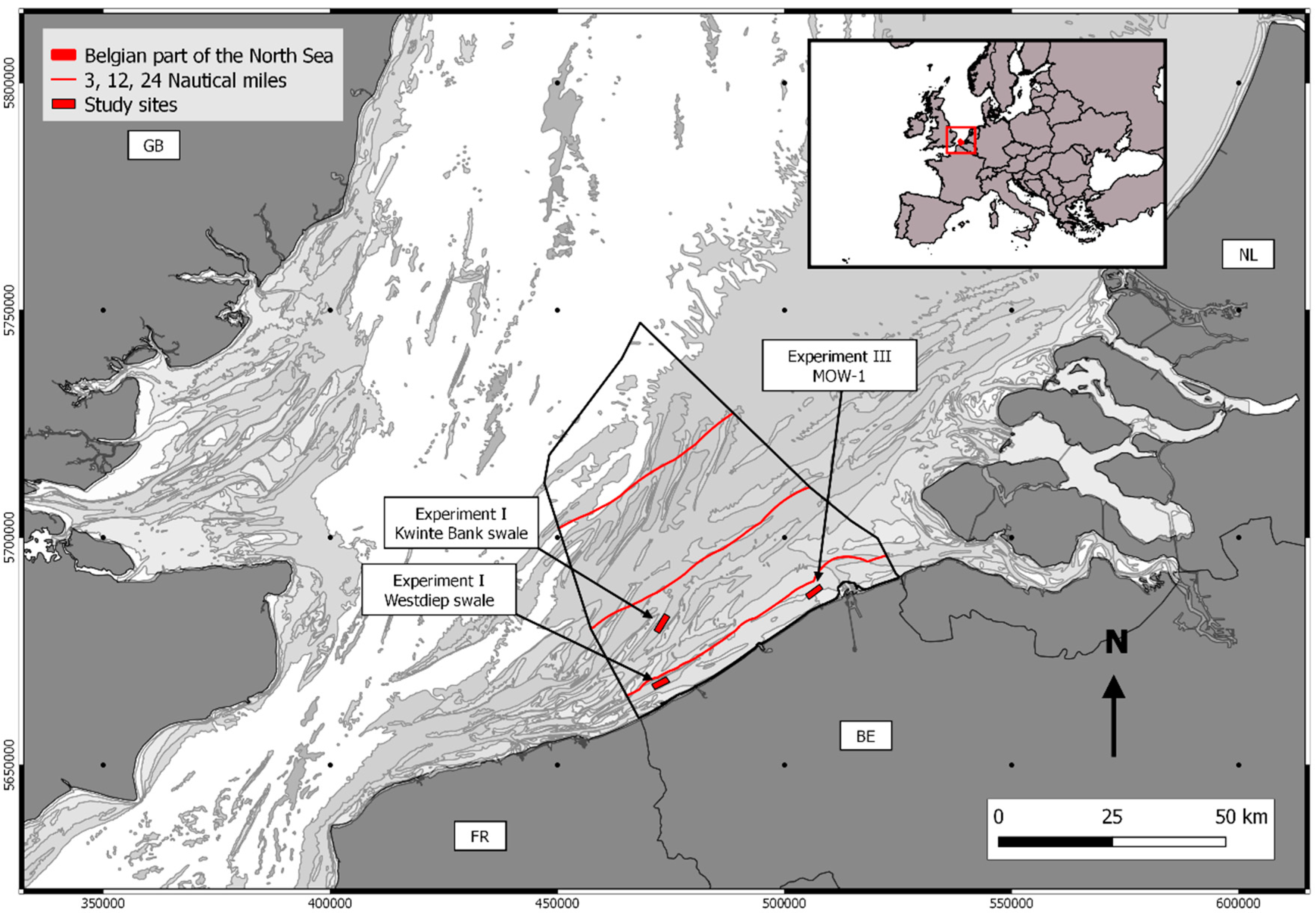
2.1. Description of MBES and Survey Areas

Multibeam data were collected using Kongsberg EM3002D and EM2040D echosounders, respectively installed on RV A962 Belgica (http://odnature.naturalsciences.be/belgica) and RV Simon Stevin (http://www.vliz.be/en/rv-simon-stevin). Table 1 reports the parameters used to operate the echosounders during the experiments.
Three surveys were conducted during spring-tide regime: in February 2015, March 2016 and November 2017, respectively on the Kwinte swale, Westdiep swale and MOW 1 areas, featuring distinct seafloor substrates. Locations are displayed in Figure 1 and general environmental conditions are given in Table 2. Within the areas, study sites were selected with homogeneous acoustic signatures, based on previous surveys and ancillary data.

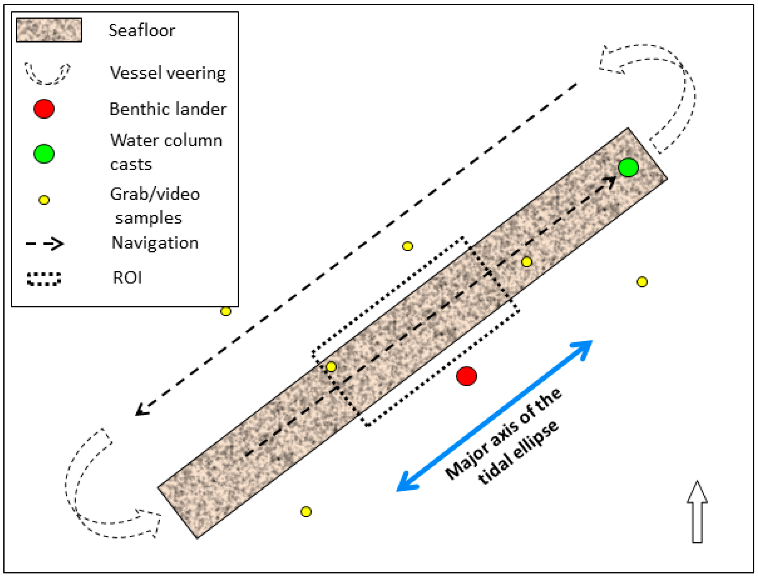
2.2. Survey Methodology and Data Processing

The surveying principle designed to capture short-term backscatter variability over the same seafloor patch is presented in Figure 2. It consists of a series of repetitive MBES measurements performed over the duration of a tidal cycle (~13 h). The same reference survey-line (~2 km) was followed using the same heading and crossing the centre of a region of interest (ROI—approximately 500 × 200 m for the first two experiments and 200 × 50 m in the third one). While deviations from the planned track line could happen for several reasons, this did not occur significantly during the experiments, and the homogeneity of the selected ROIs ensures the spatio-temporal consistency of the data across all insonified angles. Runtime acquisition parameters used in the Kongsberg Seafloor Information System software suite [53] were kept rigorously unchanged throughout the duration of each experiment, avoiding introducing extra sources of variance in the data.
Each experiment consists in the acquisition of a short-term backscatter and bathymetry time series according to the described strategy. To interpret the acoustic data, different strategies were put forward to quantify environmental variables during the experiments; these are listed hereafter for each experiment.

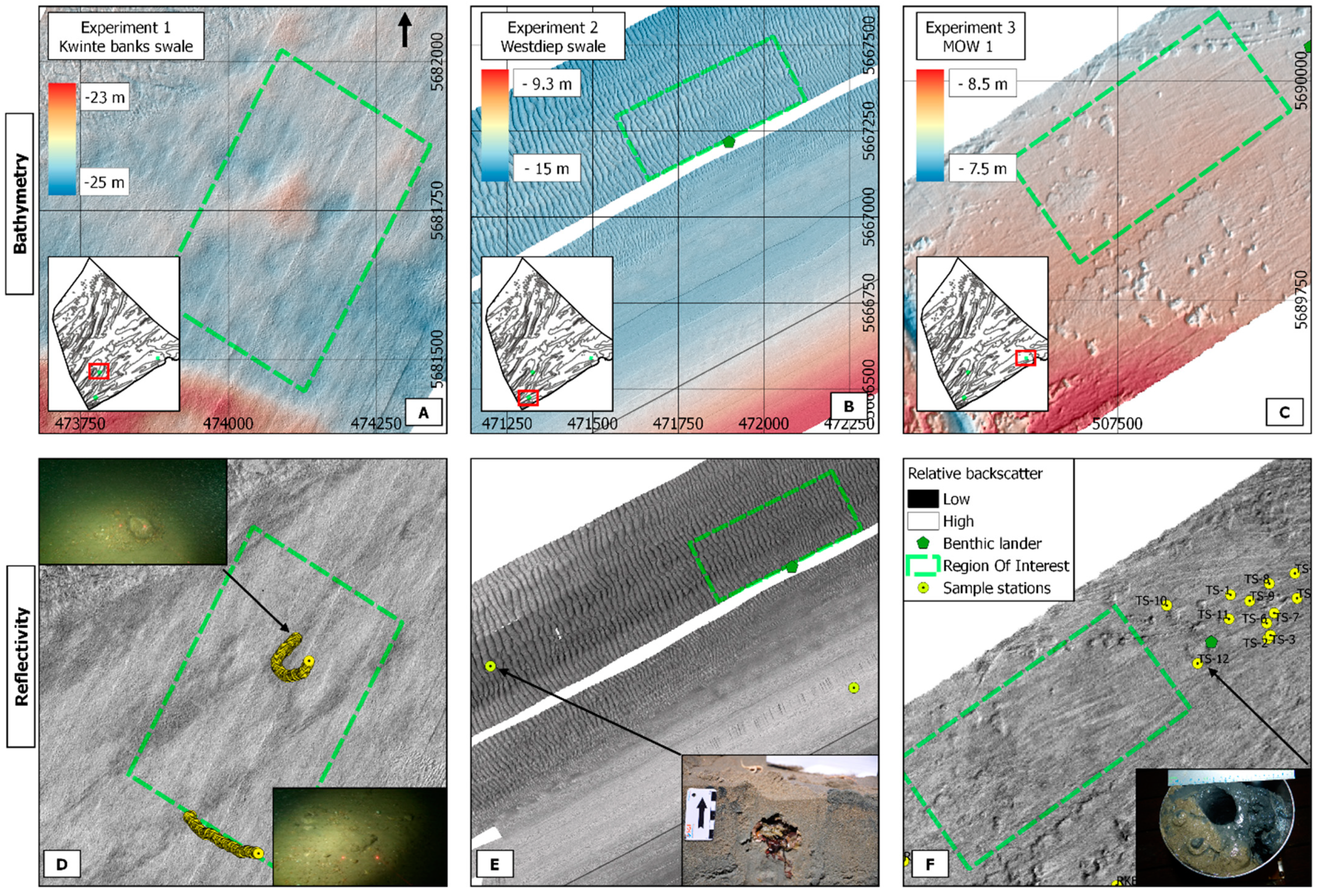
2.2.1. Experiment 1—Kwinte Swale Area

The first experiment alternated MBES measurements with vertical profiling of oceanographic variables using a drop-down frame over a 13-h tidal cycle. The area was selected because of its high stability in MBES-measured BS, based on previous investigations. Meanwhile, this site was proposed as a natural reference area to control the BS stability prior to any surveying operation in the Belgian Part of the North Sea (BPNS) [30]. The oceanographic data relating to this experiment are discussed in [33,54]. They show negligible effects of water-column processes and of near-bed sediment transport on the backscatter measurements. Here, only the MBES data are discussed.

2.2.2. Experiment 2—Westdiep Swale Area

The second experiment was extended with the deployment of a benthic lander equipped with oceanographic sensors (Figure 3; Table 3) from which variables relating to the lower ~2.4 m above seabed (mab) were derived. The lander was moored at ~120 m distance from the nadir of the MBES track line. This was the minimum distance allowed to keep a safe navigation buffer from the instrument’s signalling buoy. Given the similar morpho-sedimentary characteristics over the survey area, the information sampled by the lander was considered as representative of the processes occurring within the MBES ROI.
Measurements of suspended particulate matter concentration (SPMc) were derived using optical and acoustic backscattering sensors (OBS and ABS). Field calibrations of the OBS were carried out during previous RV Belgica cruises following the methodology described in [55]. Despite the calibration locations being different, derived SPMc are sufficiently representative of water-column processes occurring at 2.35 mab in the current study area. The multi-frequency ABS was equally used to determine SPMc, as well as median grain size (D50), in a 1-m profile above the bed and per bins of 1 cm. This sensor was chosen due to its suitability to measure in sandy environments. Calibration is provided by the manufacturer (implicit calibration methods; see [56]), and is based on the use of glass spheres being representative of quartz/siliciclastic particles present in this study area. Along with MBES and benthic lander data, an SBE 19+ SeaCAT Profiler CTD, equipped with a 5L Niskin bottle, was regularly down-casted at the end of the MBES transect to obtain measurements of SPMc, salinity, depth and temperature in the water column up until ~3 mab. This was performed approximately every hour. From each water sample, three sub-samples were filtered on board using pre-weighed filters (Whatman GF/C type). In turn, they were subsequently washed with 50 mL of Milli-Q water to remove salt, dried and weighted to derive SPMc. MBES and all benthic lander data were referenced to a uniform timestamp (the mean time of acquisition within the defined ROI) to enable later inter-comparison.
Additionally, a set of reconnaissance Van Veen grab samples (n = 7, replicate = 3) were acquired in the surroundings of the experiment site and were analysed for grain size by means of a Malvern Master-sizer 3000 (www.malvern.com). Before the analysis, organic matter and calcium carbonate (CaCO3) were removed using H2O2 (35%) and HCl (10%), respectively. To describe sediment types, the Folk and Ward [57] nomenclature is used throughout the rest of the document.

2.2.3. Experiment 3—Zeebrugge, MOW 1 Pile Area

The third experiment was carried out in the proximity of a fixed monitoring station (MOW 1—http://departement-mow.vlaanderen.be) where a benthic lander is deployed regularly by the Royal Belgian Institute of Natural Sciences as part of a long-term sediment dynamics monitoring programme [48]. The benthic lander allowed obtaining SPMc from a set of turbidity meters installed at 0.3, 1 and 2.4 mab. The OBS signals were related to mass concentration after calibration using mass-filtered water samples, taken during a 13-h tide cycle.
Furthermore, during this experiment, a time series of Reineck box cores was also collected to quantify changes in surficial sediment composition over the duration of the experiment. Overall, 12 samples were collected (approximately one every hour). They were taken from a relatively homogeneous seafloor patch and within a buffer zone with a radius of ~100 m. Particle sizes were analysed, and their nature was described as specified in the previous section. To obtain data relating to the immediate seabed surface of the samples, a 1-cm slicing was carried out on-board; the first three centimetres were kept for analysis.
Additionally, two full-coverage surveys (covering approximately 350 m × 1.5 km) were acquired over this study site on 21 and 24 November 2017 (experiment taking place before the second survey on the 24th November). Similarly to the acquisition of the time-series datasets, surveys were conducted by maintaining fixed runtime parameters and following the same set of navigation lines. Furthermore, both surveys were carried out during the same tide-window: around peak ebb flow. Following a routine to objectively find the statistical number of classes in the datasets (i.e., Within Group Sum of Squared Distances plot), maps were classified using the unsupervised k-means clustering algorithm [58] and assessed for changes by means of simple algebraic change detection (i.e., image differencing). This was carried out to appraise the short-term spatial sediment dynamics of the study area.
Considering the muddy and soft nature of the water-sediment interface of this study site and the chance to have ephemeral deposition of unconsolidated sediments [49], the Kongsberg Quality Factor (QF) was computed within the ROI to assist in the interpretation of the BS temporal/tidal oscillation. The QF is a metric relating to the relative bathymetry uncertainty and is expressed by the ratio between the scaled standard deviation of the range detection divided by the detected range [59]: the smaller the QF values, the smaller the uncertainty, implying a more accurate bottom detection. In this instance, the QF can be interpreted as a proxy of changes in the water-sediment interface, and thus for variability/sensitivity of the BS. Values of SPMc and QF are later related to the MBES BS time series by means of correlation and regression analysis.

2.3. MBES Processing

Different BS products were derived from the Kongsberg datagrams by using different software tools. All BS data were taken within the selected ROIs. Similarly to the acquisition phase, a rigorous standardized processing procedure was maintained to avoid variability induced by changes in software parameters [30]. Using the QPS FMGT© module [60], time series of 1-m horizontal resolution mosaicked backscatter were produced. The default FMGT Geocoder compensation algorithm compensates the data over the angular interval from 30° to 60°. Secondly, using the SonarScope© software suite [61], time series of AR curves were derived from the Beam intensity datagrams. The seafloor angular backscatter strength is computed from the following sonar equation liking the transmitted and received signal levels with the transmission losses and the backscattering process:
EL (R, ϴ) = SL + DTR (ϴ) − 2TL (R) + 10 log A (R, ϴ) + BS (ϴ),
where EL is the Echo Level (referenced to 1 µPa) measured at the receiver as a function of the sonar-to-target range R and the angle of incidence ϴ of the signal onto the seafloor, SL is the Source Level (in dB re 1 µPa @ 1 m), 2TL is the two-way Transmission Loss accounting for both geometrical spherical spreading (i.e., 40 log R) and absorption (2αwR—see [40,41]), A is the instantaneously insonified area, delimited by the MBES beam aperture and/or signal duration, and BS is the Backscatter Strength of the seafloor target at the observation angle ϴ. The data reduction scheme relating to the AR data-type is reported in Table 4 and, despite being relative, is considered to be the best estimate of the raw BS angular response [28,30]. Figure 4 shows the differences between AR prior and after removing the Kongsberg built-in Lambertian and specular adaptive corrections (the latter is removed a priori in the SonarScope® processing workflow). Time series of bathymetry for each experiment were also derived using QPS QIMERA© [62]. Tidal corrections using data from the closest tide-gauges were applied for the EM3002D datasets whereas a higher accuracy RTK (Real Time Kinematic) correction was applied to the EM2040D data.
The bathymetric time series were needed to assess morphological changes from 2D-depth profiles and 3D visualisation (for example between ebb and flood tidal phases). The vertical accuracy (at a 95% confidence level from descriptive statistics of the conducted measurements) of the EM3002D is ±4 cm, similarly to the value reported in [63] and compliant with the accuracy obtained by the Continental Shelf Service of Belgium conducting periodically repeated measurements over a lock situated in the harbour of Zeebrugge and where the absolute depth is known. The vertical accuracy for the EM2040D data is yet not determined. Its IHO confidence interval ([64]) is around ±15 cm, which is too large to account for decimetric vertical changes. A 1-m pixel horizontal resolution was chosen as a good balance between the size of the insonified area at nadir and that insonified at shallow grazing angles.

2.4. Transmission Losses
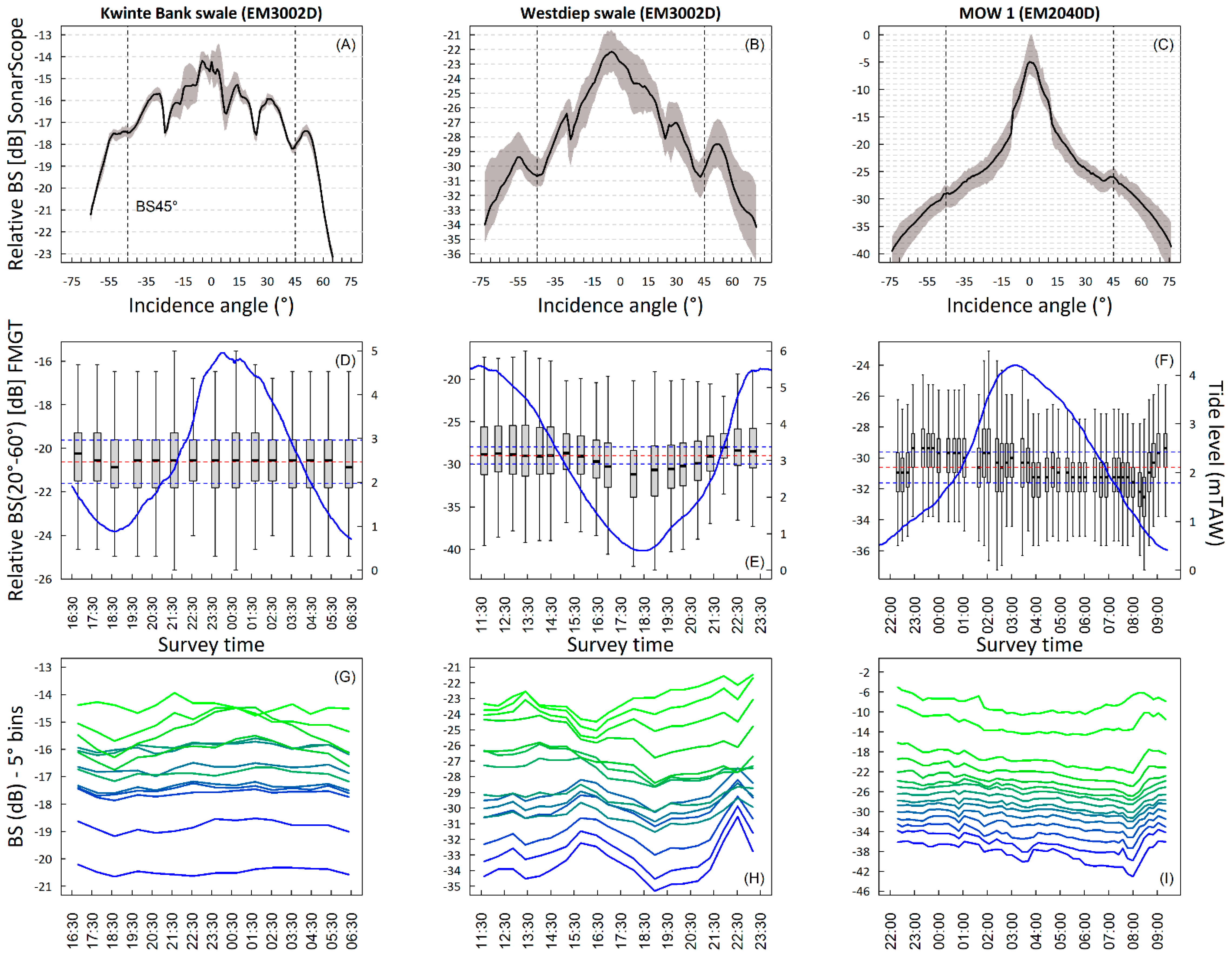
Different mechanisms beyond the inherent geometrical (spherical) spreading of the sound wave control the attenuation during the propagation in seawater and can be responsible for unwanted signal fluctuations and degradation of the signal-to-noise ratio [12]. Retrieval of the correct target backscatter strength must account on the dissipative nature of the seawater medium absorbing part of the acoustic energy via chemical reactions, viscosity and scattering [12]. Overall, attenuation losses (i.e., accounted by empirically derived absorption coefficients within the 2TL term of the sonar equation) result from the contributions of: (1) absorption in clear seawater (αw) sensu [40,41] and (2) viscous absorption (αv, [65]) and (3) scattering due to the presence of suspended particulate matter (αs, [43,66]).
The uncertainty introduced by the attenuation of sound (in dB/km) in seawater only was estimated for each experiment for nadir (0°), oblique (45°) and fall-off angular regions (70°). For the second experiment, the absorption model by [40,41] was applied to the set of water-column profiles (n = 10) obtained by the CTD frame down-casts; for the two other experiments, only surface values of absorption coefficient were considered.
Using the modelling approach in [43,66], sound absorption due to presence of suspended sediment (that due to combined viscosity and scattering) was estimated for the second and third experiments based on the available data (the routine was implemented in MATLAB©). For the second experiment, this uncertainty was estimated for the 1-m profile above the seafloor using the vertically averaged ABS-derived SPMc and median particle size (D50) for the duration of the experiment.
Additionally, uncertainty was estimated along the quasi-continuous sediment profile (~15 m depth) that was reconstructed combining observations from the various sensors (i.e., filtrations from the Niskin samples and the benthic lander mounted OBS and ABS sensors). The profile was reconstructed, and assumptions were made to represent a worst-case scenario, thereby selecting the data from the moments of maximal volume concentration. As such, the profile relates to 0.05 g/L from surface to 3 mab, 0.1 g/L from 3 to 0.5 mab and 0.3 g/L from 0.5 to seafloor. To appraise the effect of particle size, the D50 of the lower part of the profile was altered from 100 to 400 µm (reflecting the sand particles potentially resuspended in the near-bed of this area during spring tide). Despite a lack of data necessary to carry out a similar analysis in the third experiment, the available OBS-derived SPMc time series were coupled to the MBES BS by means of correlation analysis and further descriptive plots to observe relationships. Nonetheless, similarly to the second experiment, the effect over the full water depth was estimated by reconstructing a quasi-continuous sediment profile based on values of volume concentration from the OBS chain and using a fixed D50 of 63 µm (representative of suspended mud particles, characterising the turbidity of this area). Peak concentration values where selected here too, leading to a reconstructed profile of 0.2 g/L from surface to 2.5 mab, 1 g/L from 2.5 to 0.5 mab and 2 g/L for the lowest 0.5 mab. The effect of particle size was investigated here too, changing the D50 of the lowest part of the profile from 63 to 125 µm (approximating to the fine sand observed in the grab samples). For both cases, the transmission losses due to this factor are presented for nadir (0°), oblique (45°) and fall-off angular regions (70°) and for the described profile arrangements (overall 4 for the second experiment and 2 for the third one).

3. Results

3.1. Results Display

This section presents the results of the three experiments. First, the spatial context is provided through gridded backscatter and bathymetry data products. Next, a synthesis is given on the short-term variability in the backscatter time series. Interpretation of the results is helped by the ground-truth data collected for experiments II and III: for the second experiment, the benthic lander data were summarized and used to produce a set of correlations between backscatter and variables; for the third experiment, interpretation of the BS spatio-temporal behaviour is supported by a Reineck-box core time series, the SPMc obtained by the OBS chain (n = 3, at: 0.3, 1 and 2.4 mab) on the benthic lander, the bathymetric uncertainty metrics and the full-coverage surveys acquired. For each experiment, results relating to the transmission losses are presented in a separate section.

3.1.1. Offshore Gravelly Area—Kwinte Swale

Figure 5A,D shows details of the bathymetry and the backscatter, respectively, for the Kwinte swale area. Sampling stations are also shown in this image (yellow circles). The sediment of this area is medium sand with gravel and bioclastic detritus and the seafloor presents a hummocky/hillocky terrain typical of predominantly gravelly and shelly substrates of gullies (thalwegs) found in between the sandbanks of the BPNS. These substrate features were observable from the video imagery to be homogeneously distributed (with sporadic occurrence of boulders). The backscatter image for this area (Figure 5D) is moderately uniform and presents a relatively high reflectivity throughout. The patterns observable relate to the tidal-ellipse orientation (SW-NE) that follows the main axis of the gully within which the site is situated [67].
The results of repeated MBES data acquisition in this area are shown in Figure 6 (first column). The AR and boxplot time-series plots (Figure 6A,D) denote the high stability of the sediment backscatter in the area over the duration of the tidal cycle. No trend is detectable. The interquartile range is about 2 dB, indicating a high homogeneity. The consistency of the time series (Figure 6A,G) indicates that the short-term backscatter variability remains <0.5 dB across all incidence angles, except for the specular angular region (0°–18°) where the backscatter variability reaches up to ~2 dB. This behaviour is likely explained by a dependence related to the oscillations of micro-ripples (polarization under hydrodynamic forcing) which are beyond the imaging capability of the MBES spatial resolution. Figure 6J illustrates this behaviour as the AR curves at peak ebb and flood diverge more importantly in the specular angular region but converge above 25°. Interestingly, since the variability in the specular region is limited to an angle around 18°, it does not affect the mosaic production in FMGT Geocoder engine, which compensates the data based on an angular interval ranging from 30° to 60°. Small depth differences (Figure 6M) remain within the vertical accuracy of the soundings, with only slight differences in profile indentation: this is likely indicative of a polarization (and/or geometrical reorganization) of the micro-roughness under the effect of bottom currents.

3.1.2. Nearshore Sandy Area—Westdiep Swale

Bathymetry and backscatter maps for this area are presented in Figure 5B,E, respectively. The backscatter is relatively homogeneous, although a detailed inspection of the ROI indicates slight variations in backscatter values (~3 dB) between troughs and crests of the mega ripples. This may be indicative of variations in sediment type (granulometric differences) leading to finer fractions in the troughs and coarser ones on the crests and slopes. Figure 8 shows the inverse trend between depth and reflectivity profiles within this ROI. The mega ripples are flood-dominated and are oriented perpendicular to the coastline. In terms of substrate and morphology, this study area can be divided into two distinct sub-areas: the northernmost part (within which the ROI is situated), composed of well- to moderately sorted fine to medium sand and characterized by flood-dominated mega ripples (λ = ~20 m, H = ~0.8 m—see Figure 6N) and the southern part (moving coastward), where ripples become progressively smaller (λ = ~13 m, H = ~0.3 m) evolving into a very flat (<1°) area, mostly composed of well-sorted medium to coarse sand. While some biological content was present in the northernmost grab samples, considerable amounts of benthic biota were present in the remaining samples. Benthic flatfish, bivalves (Macoma baltica, Linnaeus 1758) and abundant (>10 per sample) echinoderms (Echinocardium cordatum, Pennant 1777) and brittle stars (Ophiura sp) were predominant. High bioturbation characterizes this area which may lead to important modifications of the water-sediment interface over short temporal scales.
The 13-h time series for this site is presented in Figure 6 (second column). In contrast to the very stable Kwinte swale study site, the AR time series for the Westdiep (Figure 6B,H) present very high variability throughout all angles, reaching >3 dB for the entire angular sector (BS0–73°) and >2 dB in the oblique sector (BS30–50°; Figure 6H). The trend observed in BS (Figure 6E) partly follows the oscillation of the tidal level with a significant and progressive (starting from T8, ~15:00) decrease in mean BS during the ebbing phase of the cycle. During both flood events values remain stable and fluctuate within a ±1 dB range. While the backscatter dependence due to survey azimuth was counteracted by the mono-directional survey strategy, a strong dependence to morphology is observable in this study area and is confirmed by 3D visualization of the mega ripples (Figure 7 and Figure 8). A pattern of ripple-cap inversion between flood and ebb tide flows is observed (Figure 6N), leading to build-up of finer material on the stoss side of the ripples (note the red dashed line in Figure 7, right). This is visible in Figure 6N where the ebb-phase profile shows an accretion (denoted by the white space between the vertical accuracy envelopes) of ~6 cm.
For this experiment, several physical processes were captured by the oceanographic sensors mounted on the benthic lander (Figure 9). They provide ground-truth information to understand the dynamics during the experiment and possibly to explain the observed patterns in the MBES-BS data. Non-parametric correlation coefficients obtained by the Spearman ρ rank method are presented in Table 5. While correlation may not directly imply causation, it might be indicative of the processes that drive the variability of the MBES BS at the study site in association to the hydrodynamic forcing. First, significant correlations between the mean MBES-BS, tidal level (ρ = −0.56, p < 0.05) and the current speed (ρ = 0.59, p = < 0.01) were found, suggesting that hydrodynamic-related processes played a role in the MBES-BS signal fluctuation. Significant correlations with SPMc at ~2.4 mab (from OBS and LISST sensors; ρ = −0.66, p ≤ 0.01 and ρ = 0.84, p ≤ 0.0001 respectively) were also detected. SPMc was however insufficient to explain the presence of a significant (i.e., >1 dB) absorption event and these correlations are likely indicative of a similarly fluctuating behaviour of the variables. Continuing, the vertical current velocity (in the z axis measured at 0.2 mab) and the alongshore current vector were also significantly correlated with the mean MBES BS with ρ = 0.75, p = < 0.001 and ρ = 0.58, p = < 0.01, respectively. This could be explained by the influence of the alongshore hydrodynamic forcing (the cross-shore correlation was weak and not significant) on the sand transport at the boundary layer, modifying the geometry of the bedforms and thus the resulting mean backscatter. Seabed altimetry (measured by the ADV sensor at 0.2 mab) correlated with ρ = 0.54, p = < 0.05.
The tide-level trend over the duration of the experiment is reported in Figure 9A, along with its corresponding current velocity. In this area, the amplitude of the spring tidal range is around 5.42 m with both ebb- and flood-peak tidal phases having velocities greater than 0.4 m/s, which can resuspend material [68]. Van Lancker [47] estimated the median particle size able to be resuspended and transported by subtidal alongshore flood and ebb currents in this area being respectively 420 µm (medium sand) and 177 µm (fine sand) under the spring tidal regime. The NE-directed alongshore current vector (Figure 9B) is the dominant component of the flow in this study and is the main driver of sediment mobility and geometrical reorganization of the micro-roughness. This is illustrated by the tidal ellipse (Figure 9C), which presents a SW-NE elongated shape. The vertically averaged ABS SPMc (for the 1 mab profile; Figure 9D) is in close agreement with the tidal level where highest concentrations are observable during both flood tide events (Figure 9A) reaching peak current velocities of up to 0.6 m/s in the alongshore direction (Figure 9B). Potential of deposition/erosion events during the experiment may be assessed by the combined observation of the D50 vectors (from LISST and ABS—Figure 9F,G respectively), seabed altimetry (Figure 9H), and the alongshore current (Figure 9B). During the first slack water window (around 16:00), larger median grain sizes in the suspended sediment are detected reaching ~160 µm and 220 µm, respectively, for ABS and LISST sensors (Figure 9F,G). In the following ebb phase (~19:00), under a significantly weaker alongshore ebb current velocity of about 0.2 m/s, the suspended finer matter may aggregate, sink and settle to the bottom, remaining trapped until the next flood phase (particularly considering the flood-dominated orientation of the study area and the steep lee side of the mega ripples), leading to a ~2 cm difference in seabed altimetry (Figure 9H) and a slight increase in turbidity during the ebb tide (note the OBS SPMc peak around 19:00 in Figure 9E). While this study site is situated beyond the far-field of the turbidity maximum zone, pre- and in-survey meteorological conditions induced a rather turbid ebb flow compared to the flood-incoming water masses (observations based on time series of satellite derived total suspended matter: not shown here). This may possibly introduce fine matter residue into the sandy system [48]. Nevertheless, Figure 9I indicates that throughout the experiment, the water column at ~3 mab (and presumably above this level and up to the surface) was very clear with maximal SPMc of ~0.05 g/L.

3.1.3. Nearshore Muddy Area—Zeebrugge, MOW 1

Bathymetry and backscatter maps for this area are presented in Figure 5C,E, respectively. The substrate type here is muddy sand with the sand part being <200 µm (fine sand). The bathymetry is very flat with <30 cm depth difference within the ROI (Figure 6O). Both in the backscatter and bathymetry images there is evidence of bottom trawling, resulting in regularly spaced striped depressions all over the area. In the immediate proximity of these trawl marks, erosional features appear as relatively small (5 to 15 m in diameter and ~30 cm in depth) concentric/elliptical scours, corresponding to patches of substrate being eroded and washed from the bed likely as a direct consequence of fishing gears’ passage enhanced by local hydrodynamic forcing.
The 13-h backscatter time series for this area is presented in Figure 6 (third row). Similarly to the Westdiep site (2nd experiment), the average backscatter fluctuates significantly beyond the ±1 dB sensitivity threshold and a trend consistent to the tidal oscillation is observable (Figure 6F). This study area reaches the highest level of variability: the envelope of variation exceeds 4 dB at 45° and respectively 5 and 7 dB in the specular and fall-off regions (Figure 6C,I). Higher BS averages occur around the end of the first ebb (~23:00–00:00) and around peak time of the second ebb phase (09:00—interestingly this occurs in concurrence to the higher percentages of sand fraction in the Reineck samples shown in Figure 10A and the strongest ebb current >0.5 m/s). Lower BS averages occur noticeably during the second ebb tide phase, at around slack water time (~08:00).
The interquartile range of the backscatter is about 2 dB (Figure 6F). Comparing angular responses from peak ebb and flood tidal moments (Figure 6L), no azimuthal dependence is detected (no changes in shape) confirming the absence of organized roughness in this flat area (see the 2D profiles in Figure 6O). Despite the shape of the curve remaining unaltered between ebb and flood, differences >2 dB are observable across the full angular range (i.e., a general decrease in reflectivity; Figure 6L), suggesting the transition of this seafloor patch to different states during different phases of the tidal cycle. A set of ground-truth data is presented in Figure 10 to help interpreting the MBES-BS time series. Figure 10A shows the fine sand (≤ 200 µm) and mud (≤ 63 µm) fractions from the first centimetre of the time series of sliced Reineck box core samples (12 samples, 1 approx. every hour). The tide level (blue line) is superimposed together with the corresponding current velocity (black line—from an ADP sensor). During the two ebb-tide phases, prior to slack water, the sand fraction in the samples is globally more important than during the flood tide where, in concurrence to a decrease in current velocity, samples are dominated by mud (up to ~75% content).
Figure 10B shows the bi-temporal image differencing change detection between maps of 21 and 24 November 2017 (pre- and post-experiment) summarized into 3 categories of persistence and from-to transitions between mud and sand fractions. While persistence is the dominant component of the change, the sand-to-mud change is observable at the central part of the study area where it forms an elongated pattern (where the bathymetry presents a slight channeling depression compared to the surrounding). The mud-to-sand pattern appears as more randomly distributed, forming patch-like features.
In Figure 10C, SPMc from the OBS chain, and the mean MBES BS and QF of the ROI are displayed. Again, the MBES BS acquires a most absorbing character when the SPMc reaches its maximum (around 08:00; ~2.8 g/L at 0.3 mab, 1.3 g/L at 1 mab and ~1 g/L at 2.4 mab) and reversely. The relationship between the mean MBES BS and the near-bed SPMc can be captured by a least-square linear regression (R2 = 0.47, p < 0.01) that is significant, as well as by the Spearman correlation coefficients (Table 6). Visualization of these data (Figure 10C) indicates that the least accurate sonar bottom detections (red line) occurred concurrent to the highest SPMc (particularly at 0.3 mab), resulting in the lowest BS averages. Oppositely, during the flood phase of the tide (~T13 to T18—01:00–03:00) the accuracy of the bottom detection increases with decreasing SPMc. This suggests the presence of a dynamic high-concentrated mud suspension (HCMS). Once settled, this could increase the volume of the water-sediment interface (forming a “fluffy” layer which increases the burial volume of the seafloor surface) to which the registration of bottom detection and echo intensity are sensitive to. As such, under this configuration, the active seafloor target considered in bottom detection will change from an extended surface (i.e., the relatively “clean” seafloor surface), to a volume cell (i.e., a “slice” or a truncated prism) populated by point-scatterers, which may raise or attenuate the BS level [12]. The behaviour of this HCMS layer appears as the dominant driver of variability of the MBES-BS time series of this area, leading to short-term and progressive changes in scattering mechanisms (i.e., from a relatively “clean” surface with >50% of sand to a relatively “chaotic” mixed sediment interface topped by a ~30 cm deposition of fluffy material).

3.2. Transmission Losses

In this section, transmission losses during the experiments are evaluated. The variability of the seawater absorption coefficient [40,41] was computed based on surface temperature and salinity from SBE 21 SeaCAT Thermosalinograph values stored in ODAS (On Board Data Acquisition System; R/V Belgica) and from SBE 21 SeaCAT Thermosalinograph and SBE 38 Sea-Bird Digital Oceanographic Thermometer values stored in MIDAS (Marine Information and Data Acquisition System; R/V Simon Stevin) systems. The echo level uncertainty (in dB) was estimated for the average depths of the study sites and for different slant ranges corresponding to nadir (0°), oblique (45°) and grazing (70°) angles (see Table 7). The uncertainty magnitudes resulted as negligible (N) for beams at nadir and small to negligible (S-N) for beams at 45° and 70° (according to the nomenclature proposed in [69]).
For the second experiment (Westdiep area), a set of CTD down-casts allowed investigating in more detail the absorption variability over the water-column profile. Figure 11A–D shows the vertical variability of temperature, salinity, sounds speed and αw for one CTD down-cast: the variability of these measures is within the instrumental error of the sensors, indicating the high homogeneity of the water column. Figure 11E shows the mean values of the vertically averaged absorption coefficients for each of the 10 CTD casts, individually displayed in Figure 11F. In this environmental setting, the stability of the vertical profiles justifies the use of surface values to correct for absorption during data acquisition.
For this second experiment, the SPMc and median grain size (D50) obtained from the ABS sensor (Figure 11G–H) allowed estimation of the transmission losses due to SPMc. Figure 11G reports the vertically averaged SPMc, and Figure 11H shows the dB loss for the 1-m profile. For this experiment and for such sound travel paths, fully negligible (N) influences of SPMc on the mean BS level are observed.
Nonetheless, to better appraise the uncertainty potentially introduced by this environmental factor, vertical sediment profiles (approximating to the full travel path of the acoustic signal and defined in a conservative way maximizing the SPM impact) were reconstructed for the second and third experiments as specified in the “Materials and Methods” section. As in Table 7, Table 8 reports the estimated transmission losses for nadir (0°), oblique (45°) and fall-off slant ranges (70°).
Transmission losses due to suspended sediment remain small for both experiments and for the depths, concentrations and particle sizes assessed. Noticeably, for the second experiment in the sandy and clear-water area (Westdiep swale), losses due to seawater only and those due to suspended sediment show similar magnitudes and increasing the D50 in the lower part of the water-column causes little changes. Oppositely, for the third experiment in the maximal turbidity zone, the echo level attenuation increases significantly reaching up to ~0.5 and 1 dB at oblique and fall-off slant ranges respectively, showing slight increases with increasing particle size.

4. Discussion

Mapping for monitoring requires repeated measurements of the same seafloor areas over short-, medium- and long-term time scales (i.e., diel to decadal time scales). Three field experiments were conducted in the BPNS under spring tide regime to investigate the short-term effect of environmental sources of variance on the acoustic signature of predominantly gravelly (Kwinte swale), sandy (Westdiep swale) and muddy areas (Zeebrugge, MOW 1). These field studies were also aimed at appreciating the sensitivity of the MBES-measured BS to relatively subtle variations in the nature of the water-sediment interfaces at stake. The backscatter time series were analysed, and the signatures and trends were related to seabed physical properties measured in situ, using several approaches. The potential sources of short-term (half-diel) variability that were investigated relate to: roughness polarization and morphological changes, water-column processes (transmission losses due to seawater and suspended sediment), and surficial substrate changes.

4.1. Short-Term Backscatter Tidal Dependence

The MBES-measured BS variability and its causes differed considerably between the three investigated areas. Overall, the effect of water-column absorption variability (i.e., due to seawater only), was ubiquitously negligible to small; this was expected, given the shallow depths surveyed and the good instrumental control of the local seawater characteristics. The effect of suspended sediment on the transmission losses can be expected to cause little uncertainties in the sandy and gravelly areas outside the turbidity maximum zone in Belgian waters; it could, however, become moderate to prohibitive in deeper areas or in case of dense plumes of sediments in the water column related to human activities (dredging, trawling). In general, considering jointly the seasonal and spatial variations of SPMc in the BPNS [70], a maximal water depth of ~50 m over the region, and the preliminary observations from this investigation, it may be surmised that for the gravelly and sandy clear-water areas (offshore and in the SW nearshore areas), the effect of suspended sediment will always be small, since the highest volume concentrations are to be expected in the lowest layer of the water column, thus involving too short a sound travel path to significantly affect the echo level. Previous investigations on the effect of near-bed SPM on BS for the first study area can be found in [33,54] and actually reported negligible effects. On the contrary, in the nearshore zone with soft-material sediments and maximal turbidity, significantly higher volume concentrations can be met even in the upper part of the water column, evidencing the importance of this SPM-caused attenuation even at very-shallow depths (10 m). Besides these environmental factors, the envelopes of variability were mainly driven by short-term successional changes of the underlying morphology and of the water-sediment interface physical status, thereby relating to actual changes in the targeted seafloor.

4.1.1. Experiment 1—Offshore Gravel Area

Overall, the results pointed at the high stability (<0.5 dB excluding nadir beams in the angular range 0–18°) of the Kwinte gravel area. This was expected, given the known bathymetric and sedimentological spatio-temporal stability of this area [30]. This good stability is explained by year-round, well-stratified and clear water masses [71] and possibly by an overall stochastic re-organization of the substrate (i.e., geometric micro-changes of the sand and bioclastic material) configuration under the effect of currents which limits significant alterations of the interface backscatter. The backscatter AR was here a particularly useful measurement, not only to gain a physical understanding of the backscattering characteristics of the substrate type (the AR curves show three distinct shapes characteristic of each substrate type; see Figure 6A–C), but also to detect the presence of a weak azimuthal-like dependence thanks to the BS values measured in the steep-angle range (see [39]). This would have been impossible using solely backscatter mosaics, which by nature lack the angular component (as the change detection carried out in [72,73]). This shows that a compensation of mosaicked backscatter imagery using an angular interval in the range 30°–60° (as in e.g., FMGT standard processing) would omit the azimuthal dependence (which in this gravelly/hillocky terrain extended only up until 18°) while assessing changes of interest (i.e., sediment type at oblique angles) within such seafloor types.

4.1.2. Experiment 2—Nearshore Sandy Area

The sandy area in the nearshore Westdiep swale showed significant variability (>2 dB at 45° and >3 dB over the full angular range) for the time assessed. Water-column processes here also had negligible impact. Here, most BS variability was best explained by azimuthal dependence, similarly to studies in other sandy/siliciclastic areas [28,39]. Ripple features are predominant in such areas [74] and, under the effect of both flood and ebb currents, a geometric reorganization of the morphology at various scales may occur. Wave-induced cross-shore currents, creating micro-ripples, may further contribute to MBES-BS variability; when these ripples are perpendicular to the sonar across-track acoustic line of sight, MBES-measured BS may be altered significantly (e.g., [37,38]). Besides the azimuthal dependence normally limited to steep angles [39], significant variability was also observed at angles beyond 40° (i.e., >2 dB at 45°), suggesting that some degree of sedimentary changes for the period assessed did occur. Similarly as in [75], ground-truth observations were indicative of changes at the interface that likely resulted from cyclicity in deposition/erosion events. The contribution of biological activity (i.e., bioturbation) was not quantified here but is also expected to increase the BS variability. Considerable amounts of biota were observed surrounding this study site, which aligns with previous studies [76,77]. Feeding and burrowing behaviour of certain benthic species can lead to drastic modifications of the sediment in terms of its geotechnical composition (e.g., permeability, porosity, compactness and roughness; [78]) and can therefore have large effects on the backscatter level by altering the average water-sediment impedance contrast. Furthermore, presence of individual species per se can act as surface scatterers: e.g., [16,79] related part of the high-reflectivity facies in their acoustic maps to the widespread presence of respectively the tubicolous polychaete L. conchilega and the brittle star A. filiformis modifying the micro-roughness as a function of their feeding behaviour (rising of tentacles in the water-column/boundary layer). Recently, laboratory tank-based experiments showed that in sandy sediments the effect of microphytobenthos photosynthetic activity can also introduce a variability of the backscattering properties of the inhabited marine sediment by as much as ~2.5 dB at 250 kHz and over a diel cycle [45]. This experiment demonstrates the necessity of jointly analysing mosaicked and AR BS to avoid misinterpretations of the observed changes, particularly in sandy/siliciclastic areas such as on this Westdiep area. It is worth noting that this polarization effect may raise specific (and usually underestimated) challenges when merging surveys acquired in different orientations and it will have to be considered in the compilation of existing backscatter maps.

4.1.3. Experiment 3—Nearshore Muddy Area

The MBES-BS dataset acquired near the Zeebrugge MOW 1 Pile area was by far the most variable, with a mean variability >4 dB at 45° and beyond for the remaining angular range. The variability was fully unrelated to the azimuthal dependence since the study area ground-truthing showed a levelled and relatively homogeneous terrain, lacking organized morphology. Our interpretation is rather that the variability related to a combination of the intrinsic dynamic nature of the boundary condition (creating a “fuzzy” boundary layer), to granulometric changes at the water-sediment interface (implying fluctuating fractions of sand and mud) and to a highly turbid water column. This very dynamic muddy/sandy substrate site is particularly complex from an acoustic perspective, since the sediment structure exhibits high vertical heterogeneity (i.e., an intricate layering of intercalated sediment matrix of sand and mud on anoxic mud, topped by depositions of up to 30 cm of fluffy material at specific tidal moments). This likely resulted in volumic contributions (i.e., subsurface sediment scattering) opposite to the other two experimental sites, where the impedance contrast of the water-sediment interface was significantly higher due to the presence of coarser substrates (i.e., gravel, shells and sandy-quartz sediments), and hence dominated the backscattering process. Significant acoustic penetration into the soft sandy sediments is expected to be about 2–3 cm at 300 kHz [80], increasing with softer, muddy and unconsolidated sediment as shown in this third experiment. The vertical complexity of the upper sediment layer in this area changes under the influence of the local hydrodynamic forcing that may modify at least the first 3 cm of the interface (observed from analysis of the Reineck box-core data; not shown here), as well as being subject to HCMS dynamics, that can add up to ~30 cm of fluffy material to the seafloor interface [49]. As such, different water-sediment interface configurations progressively occur during different phases of the tide and thus the echo contributions coming either from the upper layer (interface) or from the buried interface (subsurface) will together affect the bottom detection, yielding to shifts in the AR and mosaic values retrieved during the various instances. The accuracy of the bottom detection upon which depth registration relies obviously depends on how “clean” an interface is. To test this observation, the mean Kongsberg Quality Factor (QF) was processed within the ROI to complement the interpretation of the MBES-BS trend. Significant and interrelated associations were found between registered MBES BS, QF and SPMc at 0.3 mab, confirming the MBES-BS sensitivity to the boundary dynamics of this study site, as identified in [48,49]. Lastly, it should be noted that the presence of trawl marks in the ROI (see Figure 5C) may represent a further explanatory candidate of the backscatter variability. These morphological depressions would be prone to accumulation of fine material (e.g., particularly around slack tide), thereby changing the constituency of the sediment interface and influencing the BS response. The same is valid for the erosional elliptic depressions which cooccur with the trawl marks.

4.2. Recommendations on Future Experiments on MBES-BS Variability

When tidal dynamicity and/or environment seasonality are expected to cause seafloor BS variability, field studies are recommended to evaluate the significance. While the instrumentation and set-up used in the present investigation proved highly valuable for targeting this aim, some improvements could be made. Hereafter, good practice is reiterated, and shortcomings flagged. Future solutions could come in from new instrumentation and/or methodological approaches. In any case, it is critical that the surveys are conducted under favourable hydro-meteorological conditions. Table 9 shows the motion sensor-related variables during the data logging. These are used as a form of quality control on the datasets.
Noticeably, an average difference of 12° in the heading range during the first experiment could explain the slight azimuthal-like dependence observed. A similar heading average range in the third experiment has no effect in terms of azimuth given the very flat (level) seafloor. At all times during the surveys, the wave height was always lower than 1 m. Overall, the mono-directional survey strategy applied here was optimal in preventing (or at least minimizing) the effect of survey azimuth relative to the navigation heading [39]. Deviations from the planned track-line did occur for a range of reasons, but were kept minimal during the experiments. Experience showed that shorter track lines (about 1-km long) were needed to get high-density datasets enhancing the comparability and detectability of trends in the MBES BS and environmental data (n = 44 instances during the 3rd experiment, compared to n = 15 and 19 for the 1st and 2nd experiments, respectively). The use of a benthic lander device proved promising, combining various sensors on a single frame, thus retrieving multiple and relevant oceanographic data at once. However, several limitations were identified. First, there was a difference in retrieval location between the oceanographic data and the MBES data. The time bias between the measurements could in part be overcome by coupling the various data types by a unified mean time stamp (mean surveying time within the ROIs). However, the validity of this approach depends on the data acquisition periodicity by each sensor, which dictates the representativeness of the averages produced for certain tidal moments. For example, the ABS sensor used in the second experiment recorded data in bursts of 30 min, thereby possibly insufficiently capturing the sand transport behaviour at shorter time scale and possibly missing key moments of the tidal cycle (e.g., peak current velocities). Increasing and homogenising (across sensors) the frequency of registration would improve this limitation. For most optimal experiments, it is recommended to anchor the vessel on four points (i.e., port, starboard, bow and stern). This would allow collection of the various data types closer in space, as well as increase the frequency of seabed and water-column sampling by grabs and down-cast frames, thereby improving cost-time effectiveness of the experiment and data inter-comparability.
For the calculation of sound absorption due to suspended sediment in the water column, the modelling reported in [40,65] was simplified due to the limited data availability, and strong assumptions were made when vertically averaging or homogenizing the profiles. For more adequate modelling and correction of this phenomenon (e.g., in deeper clear waters where small turbidity changes may already significantly alter the BS), future experiments should collect more detailed information on concentration, particle size and vertical distribution (i.e., Rouse distribution (e.g., [81])). Uncertainty estimates due to this factor obtained by the reconstruction of full vertical sediment profiles showed that, within nearshore areas, transmission losses can vary significantly and have noticeable impact on the interpretation of multi-pass acoustic surveys. An interesting point to consider here is the rapid evolution of capabilities in water-column backscatter (WCB) data collection by modern MBES systems. Similarly to acoustic Doppler current profilers data, WCB can be calibrated against water samples to create spatially explicit profiles of SPMc and particle size, providing detailed information from near the sea-surface, down to the sonar bottom detection [82]. This raises the possibility to use more representative data and robustly implement sound-loss corrections in dynamic and deeper survey areas. Additionally, this would also be cost-effective and more complete compared to the deployment of benthic landers and associated instruments which are time consuming, labour intensive and ultimately impede the retrieval of data for the full water column.
The sonar measurements were interpreted in complement to an array of oceanographic measurements (where applicable) relating to local seafloor and water-column processes. They could be quantified by means of different equipment. Besides deploying multi-sensor benthic landers, downcast of the CTD frame allowed characterizing the water-column profile in detail, thus deriving better estimates of absorption coefficients than solely using sea-surface data. Substrate sampling gears such as the Reineck box-core, retrieving relatively undisturbed samples, proved useful to quantify short-term changes of the substrate composition, and core slicing allowed appreciating the fine-scale layering; such an instrument should be used more systematically in muddy/soft sediment areas to fully evaluate the relations between acoustic response and sub-bottom complexity. Regarding the collection of SPMc measurements, different instruments were used. Chains of OBS mounted on a benthic lander proved very useful to understand the differences between SPMc at the boundary layer (i.e., 0.3 mab) and the upper-water column (i.e., ~2.5 mab). However, they do not provide estimates of the particle size, for which a LISST and/or ABS system should be used. In any case, it is recommended that further studies are dedicated to understand the differences between optically and acoustically derived estimates and that their sensitivity to varying particle sizes and concentrations are addressed (as in [83]) so that adequacy of the instruments to different environments can be better understood.

4.3. Implications for Repeated Backscatter Mapping Using MBES

The short-term backscatter variability is only one aspect to consider when using MBES for repeated BS mapping. For the ultimate goal of merging datasets in space and time from different systems and vessels (e.g., cross-border datasets), careful consideration of multibeam system accuracy and stability, conditioning data repeatability and scaling, are required [84]. This starts with standardizing operational procedures, in terms of acquisition and processing, ideally inspired from community-driven experiences (e.g., the GeoHab backscatter working group [11]). Accuracy of an MBES system is largely dependent on the calibration process, requiring manufacturer-based operations (i.e., providing users with measurements/calibration tests results) and/or dedicated facilities and instrumentation to carry out in situ calibration (otherwise unfeasible for hull-mounted systems—see [21,29] for detailed considerations regarding calibration). Data repeatability refers to controlling the spatio-temporal consistency of the acoustic data in terms of instrumental and environment-caused drifts. Beyond direct metrological checks using dedicated equipment, instrumental drift can be controlled by repeated surveys over naturally stable areas (e.g., [29,30]) and/or fixed platforms, and regular dry-dock maintenance operations verifying the sensor status (as it is the case for the sonar systems used in this investigation). The focus of this paper was rather on the environmental drift, which refers here to evaluating the variability introduced by factors that do not directly relate to seafloor substrate type, but to water-column or near-bed sediment transport processes, as well as to target-geometry insonification related issues (i.e., azimuthal dependence, micro-scale roughness polarization). Such knowledge is important both for “snapshot in time” and for repeated mapping applications since improving the links between environmental variables and acoustic responses can improve the modelling and replication of field observations in space and time and enhance the interpretability of acoustic measurements.
It is paramount to understand the consequences of short-term environmental variability upon the interpretation of longer-term MBES-BS time series. This requires dedicated and specifically designed field experiments (e.g., this study, or the SAX experiments in [85], and those advocated in [32]).
As shown in this study, tidal periodicity and seasonality call for careful consideration, especially in shallow areas with soft-material seabeds and high sedimentary dynamics. Indeed, successive surveys of the same area may provide different information at various time scales (from day to year). In this regard, it is important that the tidal dependence is analysed per MBES-BS time series. Spotting outliers (i.e., abrupt changes in sediment response) will be relatively straightforward in the clear water and stationary areas (such as the Kwinte swale in the first experiment where tidal dependencies were low), since the magnitude of the short-term variance remains within the envelope of sensor sensitivity (i.e., the manufacturer-set ±1 dB for EM3002 and EM2040 Kongsberg systems [86]). On the contrary, the intrinsic “noisiness” (i.e., periodical variability) of the nearshore areas results in a potentially masking/blurring effect, introducing uncertainties due to the status of the water column (i.e., turbidity) or to the “mobility” of the water-sediment interface. Within such areas, the stability threshold must be defined contextually in accordance to the underlying sedimentary environment, and a transition in seafloor status can only be detected from a trend analysis on a sufficient number of serial surveys. Direction and consistency of the trend, regardless of the noise envelope, can be a valuable proxy of change and bypass conflicting results from surveys acquired at different tidal and/or seasonal moments. Interpretation of serial backscatter surveys in such environments should largely benefit both from time series of driving variables (collected via the deployment of benthic landers as in [49,70]) and from regional predictive oceanographic models providing local conditions usable for designing monitoring surveys accordingly.
In the third experiment, the observations showed that regardless of the variability or ‘noise’ on the AR curves (except for that exerted by the roughness polarization in the second experiment), the main shape of the angular behaviour, indicative of a sediment type, remained the same. While part of this variability was related to transmission losses due to suspended sediment, the observed shifts in backscatter values (a decrease in reflectivity across the full angular range between flood and ebb tide moments) was related to HCMS dynamics, which changed the water-sediment interface, evidencing the BS sensitivity to short-term and relatively subtle granulometric and volume heterogeneity changes known to occur in this area [49]. The sensitivity of the angular response to such differences in sediment composition (within the same main sediment class) was observed in several investigations. For example, in [28], the high sensitivity of AR is particularly clear: AR curves are used as the basis of classification of a large MBES dataset, resulting in an evident within-cluster variability of up to 10 dB at 45°. Further insights can be found in data presented in [87], in which different AR curves are related to varying degrees of percentage cover of coarse clastic material (i.e., shell and gravel scatterers). This suggests that from well-controlled backscatter measurements with sufficient ground truth data allowing detailed interpretation, the derived BS AR curves can capture instantaneous and temporal physical changes in substrate composition. Critical is then to decipher whether the change was naturally or anthropogenically driven, requiring knowledge of the magnitudes of short-term and seasonal variability. A priori knowledge of the magnitude of natural variability would largely assist such interpretations.

5. Conclusions and Future Directions

This research focused on the reliability/utility of BS field measurements by ship-borne MBES for the monitoring of the seafloor interface. More specifically, the aim was to study short-term BS fluctuations specifically associated with tidally induced half-diel variations of the environment. Three experiments were conducted during which BS was acquired together with environmental variables. Results showed that the latter are important factors in explaining variations in the shape and values of the BS-AR curves and the associated imagery, with various impact levels depending on the local sedimentary configuration. Consequently, it is recommended that, beyond further investigations of the different sources of MBES data variability, detailed environmental variables are systematically collected together with settings of MBES and associated devices, as well as application of best practice in survey designing. For users and surveyors operating within tidally dominated environments (both for mapping and monitoring purposes), such experiments raise several points of interest. Assuming a stable sonar system with no instrumental drift and a rigorously standardised acquisition and processing routine, the following observations were made: (1) in relatively stable and gravelly offshore areas, characterized by clear seawater, the variability due to external sources is limited and the BS measurement confidently relates to the water-sediment interface. (2) In nearshore sandy areas, roughness polarization may occur at various scales (depending on the hydrodynamic forcing) and a joint investigation of BS mosaics and BS-AR data products are needed to confidently discern between these geometrical effects and actual sediment changes. (3) In nearshore muddy and turbid areas, the influence of suspended sediment is prone to be significant and needs to be corrected for, requiring careful sampling and quantitative estimation of water-column processes. In the absence of sampling, interpretation of MBES BS requires a minima knowledge of the variability of environmental processes, from available time-series data and /or high-resolution sediment transport and current models.

Author Contributions

Conceptualisation, G.M.-G., M.R., X.L. and V.V.L.; Formal analysis, G.M.-G., M.R., M.B., N.T. and F.F.; Investigation, G.M.-G., M.R., K.D., X.L., V.V.L., N.T. and F.F.; Methodology, G.M.-G., M.R., K.D., X.L., M.B., N.T. and V.V.L.; Project administration, V.V.L., M.R. and X.L.; Writing—Original Draft, G.M.-G.; Writing—Review and Editing, G.M.-G., N.T., M.R., X.L. and V.V.L.

Funding

This paper is a contribution to the project INDI67 (BELSPO, contract BR/143/A2/INDI67) under which Giacomo Montereale Gavazzi’s PhD is funded. Ship time RV Belgica was provided by BELSPO and RBINS–OD Nature and RV Simon Stevin by Flanders Marine Institute.

Acknowledgments

We thank the crews, commander and captain of RV Belgica and RV Simon Stevin respectively for their help during the data collection phase of this investigation.

Conflicts of Interest

The authors declare no conflict of interest.

Data Availability

Raw multibeam echosounder and associated datasets from the various sensors employed in the investigation are stored at the Royal Belgian Institute of Natural Sciences and are available upon request.

References

  1. Halpern, B.S.; Walbridge, S.; Selkoe, K.A.; Kappel, C.V.; Micheli, F.; D’Agrosa, C.; Bruno, J.F.; Casey, K.S.; Ebert, C.; Fox, H.E.; et al. A Global Map of Human Impact on Marine Ecosystems. Science 2008, 319, 948–952. [Google Scholar] [CrossRef] [PubMed]
  2. Douvere, F.; Maes, F.; Vanhulle, A.; Schrijvers, J. The role of marine spatial planning in sea use management: The Belgian case. Mar. Policy 2007, 31, 182–191. [Google Scholar] [CrossRef] [Green Version]
  3. McArthur, M.A.; Brooke, B.P.; Przeslawski, R.; Ryan, D.A.; Lucieer, V.L.; Nichol, S.; McCallum, A.W.; Mellin, C.; Cresswell, I.D.; Radke, L.C. On the use of abiotic surrogates to describe marine benthic biodiversity. Estuar. Coast. Shelf Sci. 2010, 88, 21–32. [Google Scholar] [CrossRef]
  4. Rice, J.; Arvanitidis, C.; Borja, A.; Frid, C.; Hiddink, J.G.; Krause, J.; Lorance, P.; Ragnarsson, S.Á.; Sköld, M.; Trabucco, B.; et al. Indicators for Sea-floor Integrity under the European Marine Strategy Framework Directive. Ecol. Indic. 2012, 12, 174–184. [Google Scholar] [CrossRef]
  5. Belgian State. Determination of Good Environmental Status & establishment of Environmental Targets for the Belgian marine waters, Marine Strategy Framework Directive—Art 9 & 10. Available online: https://www.health.belgium.be/sites/default/files/uploads/fields/fpshealth_theme_file/19087665/Goede%20milieutoestand-MSFD%20EN.pdf (accessed on 1 November 2018).
  6. De Moustier, C.; Matsumoto, H. Seafloor acoustic remote sensing with multibeam echo-sounders and bathymetric sidescan sonar systems. Mar. Geophys. Res. 1993, 15, 27–42. [Google Scholar] [CrossRef] [Green Version]
  7. Brown, C.J.; Blondel, P. Developments in the application of multibeam sonar backscatter for seafloor habitat mapping. Appl. Acoust. 2009, 70, 1242–1247. [Google Scholar] [CrossRef]
  8. Urick, R.J. Principles of Underwater Sound for Engineers, 3rd ed.; Tata McGraw-Hill Education: New York, NY, USA, 1967. [Google Scholar]
  9. Hughes Clarke, J.E.; Mayer, L.A.; Wells, D.E. Shallow-water imaging multibeam sonars: A new tool for investigating seafloor processes in the coastal zone and on the continental shelf. Mar. Geophys. Res. 1996, 18, 607–629. [Google Scholar] [CrossRef]
  10. Ferrini, V.L.; Flood, R.D. The effects of fine-scale surface roughness and grain size on 300 kHz multibeam backscatter intensity in sandy marine sedimentary environments. Mar. Geol. 2006, 228, 153–172. [Google Scholar] [CrossRef]
  11. Lamarche, G.; Lurton, X. Recommendations for improved and coherent acquisition and processing of backscatter data from seafloor-mapping sonars. Mar. Geophys. Res. 2018, 39, 5–22. [Google Scholar] [CrossRef]
  12. Lurton, X. An Introduction to Underwater Acoustics: Principles and Applications; Springer: Berlin/Heidelberg, Germany, 2002; p. 680. ISBN 978-3-540-78480-7. [Google Scholar]
  13. Strong, J.A.; Elliott, M. The value of remote sensing techniques in supporting effective extrapolation across multiple marine spatial scales. Mar. Pollut. Bull. 2017, 116, 405–419. [Google Scholar] [CrossRef]
  14. Brown, C.J.; Sameoto, J.A.; Smith, S.J. Multiple methods, maps, and management applications: Purpose made seafloor maps in support of ocean management. J. Sea Res. 2012, 72, 1–13. [Google Scholar] [CrossRef]
  15. Buhl-Mortensen, L.; Buhl-Mortensen, P.; Dolan, M.F.J.; Holte, B. The MAREANO programme—A full coverage mapping of the Norwegian off-shore benthic environment and fauna. Mar. Biol. Res. 2015, 11, 4–17. [Google Scholar] [CrossRef]
  16. Holler, P.; Markert, E.; Bartholomä, A.; Capperucci, R.; Hass, H.C.; Kröncke, I.; Mielck, F.; Reimers, H.C. Tools to evaluate seafloor integrity: Comparison of multi-device acoustic seafloor classifications for benthic macrofauna-driven patterns in the German Bight, Southern North Sea. Geo-Mar. Lett. 2017, 37, 93–109. [Google Scholar] [CrossRef]
  17. Madricardo, F.; Foglini, F.; Kruss, A.; Ferrarin, C.; Pizzeghello, N.M.; Murri, C.; Rossi, M.; Bajo, M.; Bellafiore, D.; Campiani, E.; et al. High resolution multibeam and hydrodynamic datasets of tidal channels and inlets of the Venice Lagoon. Sci. Data 2017, 4, 170121. [Google Scholar] [CrossRef] [PubMed]
  18. Jackson, D.R.; Baird, A.M.; Crisp, J.J.; Thomson, P.A.G. High-frequency bottom backscatter measurements in shallow water. J. Acoust. Soc. Am. 1986, 80, 1188–1199. [Google Scholar] [CrossRef]
  19. Hughes Clarke, J.E.; Danforth, B.W.; Valentine, P. Areal Seabed Classification using Backscatter Angular Response at 95 kHz. In Proceedings of the Conference of High Frequency Acoustics in Shallow Water, NATO SACLANT Undersea Research Centre, Lerici, Italy, 30 June–4 July 1997. [Google Scholar]
  20. Che Hasan, R.; Ierodiaconou, D.; Laurenson, L.; Schimel, A. Integrating Multibeam Backscatter Angular Response, Mosaic and Bathymetry Data for Benthic Habitat Mapping. PLoS ONE 2014, 9, e97339. [Google Scholar] [CrossRef] [PubMed]
  21. Eleftherakis, D.; Berger, L.; Le Bouffant, N.; Pacault, A.; Augustin, J.-M.; Lurton, X. Backscatter calibration of high-frequency multibeam echosounder using a reference single-beam system, on natural seafloor. Mar. Geophys. Res. 2018, 39, 55–73. [Google Scholar] [CrossRef]
  22. Fonseca, L.; Mayer, L. Remote estimation of surficial seafloor properties through the application Angular Range Analysis to multibeam sonar data. Mar. Geophys. Res. 2007, 28, 119–126. [Google Scholar] [CrossRef]
  23. Galparsoro, I.; Borja, Á.; Bald, J.; Liria, P.; Chust, G. Predicting suitable habitat for the European lobster (Homarus gammarus), on the Basque continental shelf (Bay of Biscay), using Ecological-Niche Factor Analysis. Ecol. Model. 2009, 220, 556–567. [Google Scholar] [CrossRef]
  24. Wedding, L.; Lepczyk, C.; Pittman, S.; Friedlander, A.; Jorgensen, S. Quantifying seascape structure: Extending terrestrial spatial pattern metrics to the marine realm. Mar. Ecol. Prog. Ser. 2011, 427, 219–232. [Google Scholar] [CrossRef]
  25. Ierodiaconou, D.; Schimel, A.C.G.; Kennedy, D.; Monk, J.; Gaylard, G.; Young, M.; Diesing, M.; Rattray, A. Combining pixel and object based image analysis of ultra-high resolution multibeam bathymetry and backscatter for habitat mapping in shallow marine waters. Mar. Geophys. Res. 2018, 39, 271–288. [Google Scholar] [CrossRef]
  26. Lamarche, G.; Lurton, X.; Verdier, A.-L.; Augustin, J.-M. Quantitative characterisation of seafloor substrate and bedforms using advanced processing of multibeam backscatter—Application to Cook Strait, New Zealand. Cont. Shelf Res. 2011, 31, S93–S109. [Google Scholar] [CrossRef]
  27. Ladroit, Y.; Lamarche, G.; Pallentin, A. Seafloor multibeam backscatter calibration experiment: Comparing 45°-tilted 38-kHz split-beam echosounder and 30-kHz multibeam data. Mar. Geophys. Res. 2018, 39, 41–53. [Google Scholar] [CrossRef]
  28. Fezzani, R.; Berger, L. Analysis of calibrated seafloor backscatter for habitat classification methodology and case study of 158 spots in the Bay of Biscay and Celtic Sea. Mar. Geophys. Res. 2018, 39, 169–181. [Google Scholar] [CrossRef]
  29. Weber, T.C.; Rice, G.; Smith, M. Toward a standard line for use in multibeam echo sounder calibration. Mar. Geophys. Res. 2018, 39, 75–87. [Google Scholar] [CrossRef]
  30. Roche, M.; Degrendele, K.; Vrignaud, C.; Loyer, S.; Le Bas, T.; Augustin, J.-M.; Lurton, X. Control of the repeatability of high frequency multibeam echosounder backscatter by using natural reference areas. Mar. Geophys. Res. 2018, 39, 89–104. [Google Scholar] [CrossRef]
  31. Roche, M.; Degrendele, K.; Vandenreyken, H.; Schotte, P. Multi Time and Space scale Monitoring of the Sand Extraction and Its Impact on the Seabed by Coupling EMS Data and MBES Measurements. 33. Belgian Marine Sand: A Scarce Resource? Belgian FPS Economy—Study day 9. June 2017. Available online: http://economie.fgov.be/fr/binaries/Articles-study-day-2017_tcm326-283850.pdf (accessed on 1 November 2018).
  32. Lucieer, V.; Roche, M.; Degrendele, K.; Malik, M.; Dolan, M.; Lamarche, G. User expectations for multibeam echo sounders backscatter strength data-looking back into the future. Mar. Geophys. Res. 2018, 39, 23–40. [Google Scholar] [CrossRef]
  33. Roche, M.; Baeye, M.; Bisschop, J.D.; Degrendele, K.; Papili, S.; Lopera, O.; Lancker, V.V. Backscatter stability and influence of water column conditions: Estimation by multibeam echosounder and repeated oceanographic measurements, Belgian part of the North Sea. Inst. Acoust. 2015, 37, 8. [Google Scholar]
  34. Singh, A. Review Article Digital change detection techniques using remotely-sensed data. Int. J. Remote Sens. 1989, 10, 989–1003. [Google Scholar] [CrossRef] [Green Version]
  35. Floricioiu, D.; Rott, H. Seasonal and short-term variability of multifrequency, polarimetric radar backscatter of Alpine terrain from SIR-C/X-SAR and AIRSAR data. IEEE Trans. Geosci. Remote Sens. 2001, 39, 2634–2648. [Google Scholar] [CrossRef]
  36. Boehme, H.; Chotiros, N.P.; Rolleigh, L.D.; Pitt, S.P.; Garcia, A.L.; Goldsberry, T.G.; Lamb, R.A. Acoustic backscattering at low grazing angles from the ocean bottom. I. Bottom backscattering strength. J. Acoust. Soc. Am. 1984, 75, S30. [Google Scholar] [CrossRef]
  37. Briggs, K.B.; Williams, K.L.; Richardson, M.D.; Jackson, D.R. Effects of Changing Roughness on Acoustic Scattering: (1) Natural Changes. Proc. Inst. Acoust. 2001, 23, 375–382. [Google Scholar]
  38. Richardson, M.D.; Briggs, K.B.; Williams, K.L.; Lyons, A.P.; Jackson, D.R. Effects of Changing Roughness on Acoustic Scattering: (2) Anthropogenic Changes. 2001. Available online: http://www.apl.washington.edu/programs/SAX99/IOSpapers/Richardson.pdf (accessed on 4 December 2018).
  39. Lurton, X.; Eleftherakis, D.; Augustin, J.-M. Analysis of seafloor backscatter strength dependence on the survey azimuth using multibeam echosounder data. Mar. Geophys. Res. 2018, 39, 183–203. [Google Scholar] [CrossRef]
  40. Francois, R.E.; Garrison, G.R. Sound absorption based on ocean measurements: Part I: Pure water and magnesium sulfate contributions. J. Acoust. Soc. Am. 1982, 72, 896–907. [Google Scholar] [CrossRef]
  41. Francois, R.E.; Garrison, G.R. Sound absorption based on ocean measurements. Part II: Boric acid contribution and equation for total absorption. J. Acoust. Soc. Am. 1982, 72, 1879–1890. [Google Scholar] [CrossRef]
  42. De Campos Carvalho, R.; de Oliveira Junior, A.M.; Clarke, J.E.H. Proper environmental reduction for attenuation in multi-sector sonars. In Proceedings of the 2013 IEEE/OES Acoustics in Underwater Geosciences Symposium, Rio de Janeiro, Brazil, 24–26 July 2013; pp. 1–6. [Google Scholar]
  43. Richards, S.D.; Heathershaw, A.D.; Thorne, P.D. The effect of suspended particulate matter on sound attenuation in seawater. J. Acoust. Soc. Am. 1996, 100, 1447–1450. [Google Scholar] [CrossRef]
  44. Holliday, D.V.; Pieper, R.E. Volume scattering strengths and zooplankton distributions at acoustic frequencies between 0.5 and 3 MHz. J. Acoust. Soc. Am. 1980, 67, 135–146. [Google Scholar] [CrossRef]
  45. Gorska, N.; Kowalska-Duda, E.; Pniewski, F.; Latała, A. On diel variability of marine sediment backscattering properties caused by microphytobenthos photosynthesis: Impact of environmental factors. J. Mar. Syst. 2018, 182, 1–11. [Google Scholar] [CrossRef]
  46. Bellec, V.K.; Lancker, V.V.; Degrendele, K.; Roche, M. Geo-environmental Characterization of the Kwinte Bank. J. Coast. Res. 2010, 63–76. [Google Scholar]
  47. Van Lancker, V. Sediment and Morphodynamics of a Siliciclastic near Coastal Area, in Relation to Hydrodynamical and Meteorological Conditions: Belgian Continental Shelf. Ph.D. Thesis, Gent University, Gent, Belgium, 24 June 1999. [Google Scholar]
  48. Fettweis, M.; Baeye, M. Seasonal variation in concentration, size, and settling velocity of muddy marine flocs in the benthic boundary layer: Seasonality of SPM concentration. J. Geophys. Res. Oceans 2015, 120, 5648–5667. [Google Scholar] [CrossRef]
  49. Baeye, M.; Fettweis, M.; Legrand, S.; Dupont, Y.; Van Lancker, V. Mine burial in the seabed of high-turbidity area—Findings of a first experiment. Cont. Shelf Res. 2012, 43, 107–119. [Google Scholar] [CrossRef]
  50. Lanckneus, J.; Van Lancker, V.; Moerkerke, G.; Van Den Eynde, D.; Fettweis, M.; De Batist, M.; Jacobs, P. Investigation of the Natural Sand Transport on the Belgian Continental Shelf (BUDGET); Federal Office for Scientific, Technical and Cultural Affairs (OSTC): Brussel, Belgium, 2001; pp. 104–187. Available online: http://www.vliz.be/imisdocs/publications/ocrd/262275.pdf (accessed on 1 November 2018).
  51. Van Lancker, V.; De Batist, M.; Fettweis, M.; Pichot, G.; Monbaliu, J. Management, Research and Budgeting of Aggregates in Shelf Seas Related to End-Users (MAREBASSE); Belgian Scientific Policy Office: Brussel, Belgium, 2007; p. 66. Available online: http://www.vliz.be/imisdocs/publications/139287.pdf (accessed on 5 October 2018).
  52. Davies, C.E.; Moss, D.; Hill, M.O. EUNIS Habitat Classification Revised. European Environment Agency European Topic Centre on Nature Protection and Biodiversity, October 2004. Available online: https://www.eea.europa.eu/data-and-maps/data/eunis-habitat-classification (accessed on 1 November 2018).
  53. Kongsberg Maritime. Seafloor Information System Reference Manual—429004/A, 5th ed.; Kongsberg Maritime: Kongsberg, Norway, April 2018; Available online: https://www.km.kongsberg.com/ks/web/nokbg0397.nsf/AllWeb/A269870356C3A572C1256E19004ECFA9/$file/164878ac_SIS_Product_specification.pdf (accessed on 1 November 2018).
  54. De Bisschop, J. Influence of Water Column Properties on Multibeam Backscatter. Master’s Thesis, Gent University, Gent, Belgium, September 2016. [Google Scholar]
  55. Fettweis, M.; Baeye, M.; Lee, B.J.; Chen, P.; Yu, J.C.S. Hydro-meteorological influences and multimodal suspended particle size distributions in the Belgian nearshore area (southern North Sea). Geo-Mar. Lett. 2012, 32, 123–137. [Google Scholar] [CrossRef]
  56. Thorne, P.D.; Hanes, D.M. A review of acoustic measurement of small-scale sediment processes. Cont. Shelf Res. 2002, 22, 603–632. [Google Scholar] [CrossRef] [Green Version]
  57. Blott, S.J.; Pye, K. GRADISTAT: A grain size distribution and statistics package for the analysis of unconsolidated sediments. Earth Surf. Process. Landf. 2001, 26, 1237–1248. [Google Scholar] [CrossRef]
  58. Hartigan, J.A.; Wong, M.A. Algorithm AS 136: A K-Means Clustering Algorithm. Appl. Stat. 1979, 28, 100. [Google Scholar] [CrossRef]
  59. Kongsberg Maritime. EM Series Multibeam Echo Sounders Datagram Formats—850-160692/W; Kongsberg Maritime: Kongsberg, Norway, January 2018; Available online: https://www.km.kongsberg.com/ks/web/nokbg0397.nsf/AllWeb/253E4C58DB98DDA4C1256D790048373B/$file/160692_em_datagram_formats.pdf (accessed on 9 September 2018).
  60. QPS. Available online: http://www.qps.nl/display/main/home (accessed on 12 October 2018).
  61. SonarScope—Ifremer Fleet. Available online: http://flotte.ifremer.fr/fleet/Presentation-of-the-fleet/On-board-software/SonarScope (accessed on 12 October 2018).
  62. Qimera. Available online: http://www.qps.nl/display/qimera/Home;jsessionid=DC46DBAC82D50C8F37EAFDF66AD21338 (accessed on 2 November 2018).
  63. Ernstsen, V.B.; Noormets, R.; Hebbeln, D.; Bartholomä, A.; Flemming, B.W. Precision of high-resolution multibeam echo sounding coupled with high-accuracy positioning in a shallow water coastal environment. Geo-Mar. Lett. 2006, 26, 141–149. [Google Scholar] [CrossRef]
  64. International Hydrographic Organisation. Available online: https://www.iho.int/iho_pubs/standard/S-44_5E.pdf (accessed on 2 November 2018).
  65. Urick, R.J. The Absorption of Sound in Suspensions of Irregular Particles. J. Acoust. Soc. Am. 1948, 20, 283–289. [Google Scholar] [CrossRef]
  66. Hoitink, A.J.F.; Hoekstra, P. Observations of suspended sediment from ADCP and OBS measurements in a mud-dominated environment. Coast. Eng. 2005, 52, 103–118. [Google Scholar] [CrossRef]
  67. Van den Eynde, D.; Giardino, A.; Portilla, J.; Fettweis, M.; Francken, F.; Monbaliu, J. Modelling the effects of sand extraction, on sediment transport due to tides, on the Kwinte Bank. J. Coast. Res. 2010, 51, 101–116. [Google Scholar]
  68. Soulsby, R. Dynamics of Marine Sands: A Manual for Practical Applications, 1st ed.; Thomas Telford Publications: London, UK, 1997. [Google Scholar]
  69. Malik, M.; Lurton, X.; Mayer, L. A framework to quantify uncertainties of seafloor backscatter from swath mapping echosounders. Mar. Geophys. Res. 2018, 39, 151–168. [Google Scholar] [CrossRef]
  70. Fettweis, M.; Lee, B. Spatial and Seasonal Variation of Biomineral Suspended Particulate Matter Properties in High-Turbid Nearshore and Low-Turbid Offshore Zones. Water 2017, 9, 694. [Google Scholar] [CrossRef]
  71. Van Leeuwen, S.; Tett, P.; Mills, D.; van der Molen, J. Stratified and nonstratified areas in the North Sea: Long-term variability and biological and policy implications: North sea stratification regimes. J. Geophys. Res. Oceans 2015, 120, 4670–4686. [Google Scholar] [CrossRef]
  72. Rattray, A.; Ierodiaconou, D.; Monk, J.; Versace, V.; Laurenson, L. Detecting patterns of change in benthic habitats by acoustic remote sensing. Mar. Ecol. Prog. Ser. 2013, 477, 1–13. [Google Scholar] [CrossRef] [Green Version]
  73. Montereale-Gavazzi, G.; Roche, M.; Lurton, X.; Degrendele, K.; Terseleer, N.; Van Lancker, V. Seafloor change detection using multibeam echosounder backscatter: Case study on the Belgian part of the North Sea. Mar. Geophys. Res. 2018, 39, 229–247. [Google Scholar] [CrossRef]
  74. Masselink, G.; Austin, M.J.; O’Hare, T.J.; Russell, P.E. Geometry and dynamics of wave ripples in the nearshore zone of a coarse sandy beach. J. Geophys. Res. 2007, 112. [Google Scholar] [CrossRef] [Green Version]
  75. Ernstsen, V.B.; Noormets, R.; Winter, C.; Hebbeln, D.; Bartholomä, A.; Flemming, B.W.; Bartholdy, J. Quantification of dune dynamics during a tidal cycle in an inlet channel of the Danish Wadden Sea. Geo-Mar. Lett. 2006, 26, 151–163. [Google Scholar] [CrossRef]
  76. Van Hoey, G.; Degraer, S.; Vincx, M. Macrobenthic community structure of soft-bottom sediments at the Belgian Continental Shelf. Estuar. Coast. Shelf Sci. 2004, 59, 599–613. [Google Scholar] [CrossRef] [Green Version]
  77. Degraer, S.; Verfaillie, E.; Willems, W.; Adriaens, E.; Vincx, M.; Van Lancker, V. Habitat suitability modelling as a mapping tool for macrobenthic communities: An example from the Belgian part of the North Sea. Cont. Shelf Res. 2008, 28, 369–379. [Google Scholar] [CrossRef] [Green Version]
  78. Rowden, A.A.; Jago, C.F.; Jones, S.E. Influence of benthic macrofauna on the geotechnical and geophysical properties of surficial sediment, North Sea. Cont. Shelf Res. 1998, 18, 1347–1363. [Google Scholar] [CrossRef]
  79. Degraer, S.; Moerkerke, G.; Rabaut, M.; Van Hoey, G.; Du Four, I.; Vincx, M.; Henriet, J.-P.; Van Lancker, V. Very-high resolution side-scan sonar mapping of biogenic reefs of the tube-worm Lanice conchilega. Remote Sens. Environ. 2008, 112, 3323–3328. [Google Scholar] [CrossRef]
  80. Huff, L. Acoustic Remote Sensing as a Tool for Habitat Mapping in Alaska Waters. In Marine Habitat Mapping Technology for Alaska; Reynolds, J., Greene, H., Eds.; Alaska Sea Grant, University of Alaska Fairbanks: Fairbanks, AK, USA, 2008; pp. 29–46. [Google Scholar]
  81. Zyserman, J.A.; Fredsøe, J. Data Analysis of Bed Concentration of Suspended Sediment. J. Hydraul. Eng. 1994, 120, 1021–1042. [Google Scholar] [CrossRef]
  82. Simmons, S.M.; Parsons, D.R.; Best, J.L.; Orfeo, O.; Lane, S.N.; Kostaschuk, R.; Hardy, R.J.; West, G.; Malzone, C.; Marcus, J.; et al. Monitoring Suspended Sediment Dynamics Using MBES. J. Hydraul. Eng. 2010, 136, 45–49. [Google Scholar] [CrossRef]
  83. Hawley, N. A Comparison of Suspended Sediment Concentrations Measured by Acoustic and Optical Sensors. J. Gt. Lakes Res. 2004, 30, 301–309. [Google Scholar] [CrossRef]
  84. Anderson, J.T.; Van Holliday, D.; Kloser, R.; Reid, D.G.; Simard, Y. Acoustic seabed classification: Current practice and future directions. ICES J. Mar. Sci. 2008, 65, 1004–1011. [Google Scholar] [CrossRef]
  85. Williams, K.L.; Jackson, D.R.; Tang, D.; Briggs, K.B.; Thorsos, E.I. Acoustic Backscattering from a Sand and a Sand/Mud Environment: Experiments and Data/Model Comparisons. IEEE J. Ocean. Eng. 2009, 34, 388–398. [Google Scholar] [CrossRef]
  86. Hammerstad, E. EM technical note: Backscattering and seabed image reflectivity. Horten Nor. Kongsberg Marit. AS 2000, 1–5. Available online: https://www.km.kongsberg.com/ks/web/nokbg0397.nsf/AllWeb/C2AE0703809C1FA5C1257B580044DD83/$file/EM_technical_note_web_BackscatteringSeabedImageReflectivity.pdf (accessed on 12 October 2018).
  87. Daniell, J.; Siwabessy, J.; Nichol, S.; Brooke, B. Insights into environmental drivers of acoustic angular response using a self-organising map and hierarchical clustering. Geo-Mar. Lett. 2015, 35, 387–403. [Google Scholar] [CrossRef]
Figure 1. Location of selected study sites within the Belgian part of the North Sea: (1) Kwinte swale area (central coordinate: N 51° 17.2717, E 002° 37.7035), (2) Westdiep swale area (N 51° 09.1230, E 002° 34.6806), (3) Zeebrugge, MOW 1 pile area (N 51° 21.6697, E 003° 06.5798). The inset shows the location of the Belgian part of the North Sea within the European geographical zone. Data are projected in World Geodetic System 84 (WGS 84) in Universal Transverse Mercator Zone 31 N (UTM—31N). This coordinate system is used throughout the rest of the document.
Geosciences 09 00034 g001
Figure 2. Schematic representation (not to scale) of the surveying principle designed to capture the short-term backscatter variability over a homogeneous region of interest (ROI). See main text for explanations.
Geosciences 09 00034 g002
Figure 3. (A) Benthic lander equipped with a set of oceanographic sensors (see Table 1 for details about the instrumentation) deployed during the second experiment in the Westdiep study site. A similar lander was deployed for the third experiment. A chain of OBS+ sensors at 0.3, 1 and 2.4 m above bottom (mab) was present during the third experiment. In this image: (A) Benthic lander frame, (B) laser in situ transmissometer, (C) optical backscatter sensor, (D) acoustic backscatter sensor, (E) acoustic doppler velocimeter; and on-board winch-operated instruments, (F) Van Veen grab, (G) Reineck boxcore, (H) CTD frame, equipped with a OBS+ and a Niskin bottle.
Geosciences 09 00034 g003
Figure 4. Illustration of the difference between angular response curves provided by the Kongsberg manufacturer after correction in SonarScope© to remove the specular correction (dashed line, applied by default in SonarScope© processing routine) and the Lambertian correction (solid line, backscatter status 1 in SonarScope©). The solid line is the type of angular response data used in the present investigation and is believed to be the best estimate of the raw intrinsic seafloor backscatter response. The type of BS data output particularly suits the study of variability (i.e., relying on an artefact- and bias-free dataset) since the built-in specular-adaptive and Lambertian corrections are computed on a ping-to-ping basis, hence possibly introducing biases due to the local seafloor configuration.
Geosciences 09 00034 g004
Figure 5. Details of the bathymetry (AC) and reflectivity maps (DF) for each study area. For experiments II (BE) and III (CF), the location of the benthic lander, equipped with various oceanographic sensors, is denoted by a dark-green pentagon. Ground-truth stations are denoted by yellow circles, whereas the ROIs are denoted by green dashed-line polygons. Photographic details of the substrate types are also shown: for the Kwinte swale area images (D), the laser points are 9 cm apart (Courtesy of A. Norro, Royal Belgian Institute of Natural Sciences). Severe modification of the seabed by bottom trawling gears is noticeable at the MOW 1 study site (C,F): patterns of substrate erosion (elliptical depressions of ~10 to 30 cm in depth and up to 15 m in diameter) occur in the immediate proximity of the trawl marks.
Geosciences 09 00034 g005
Figure 6. Synthesis of the backscatter time series acquired for each experiment. The first plot (AC) is the envelope of variability (grey shading) around the average AR (black line) of the full AR BS time series, extracted from the defined ROIs. It describes the variability of backscatter intensity per angle of incidence over the duration of the experiments. The envelope is computed from n = 15, 19 and 47 MBES passes respectively for the 1st, 2nd and 3rd experiment. The processing scheme code for the AR BS dataset is “A4 B1, C2 D1 E5 F3 G2 H3 I0 J0 H2” using the nomenclature proposed in [11]. The second plot (DF) is the same time series (though derived from the BS mosaics produced in FMGT; BS30-60° @ 300 kHz) but visualized as boxplots of relative BS (values across the full incidence angle) against the time of acquisition (mean surveying time within the ROI). The overall mean over the full time series, together with the ±1 dB Kongsberg sensitivity threshold [66], are respectively shown as red and blue dashed lines. The tidal level is superimposed to assess a prospective BS trend in respect to the tidal oscillation and its phases. In the boxplots, lower and upper box boundaries are the 25th and 75th percentile respectively, the black central bar the median, whiskers denote the full extent of the data (i.e., min/max). The processing scheme code for the mosaicked BS dataset is “A4 B0 C0 D0 E5 F0” using the nomenclature proposed in [11]. The third plot (G,H) is the time evolution of the relative BS for areas insonified within a same envelope of incidence angle at a 5° resolution. This provides a more detailed depiction of the variability as a function of the incidence angle, to observe if smaller angular sectors would be less affected by the processes driving the variability. In (G,H), the blue to green palette represents angular intervals from the fall-off to the specular region in steps of 5°, leading to approximately 15 sub-sectors per experiment. The fourth plot (JL) displays the AR curves at the peak flood and ebb tidal phases (the legend mentions the corresponding survey time) during the experiments and is used to establish the presence of roughness-polarization dependence (as proposed in [27,36]). The fifth plot (MO) displays bathymetric profiles extracted at nadir within the ROIs at the same peak flood and ebb tidal moments as the previous plot (JL). For the Kwinte swale and Westdiep experiments, using the EM3002D echosounder, the ±4 cm vertical accuracy interval is displayed as a grey/transparent envelope.
Geosciences 09 00034 g006aGeosciences 09 00034 g006b
Figure 7. 3D models of a mega ripple found within the ROI of the Westdiep experiment (central ripple in Figure 6N; same peak flood and ebb times as in Figure 6K). Vertical exaggeration = 6×. To verify the consistency of this pattern over the entire study area, profiles were extracted from the full transect; different sub-areas of the entire transect and at different angles i.e., nadir, oblique and fall-off angular regions of the swathe (not shown).
Geosciences 09 00034 g007
Figure 8. 2D profiles of bathymetry and backscatter extracted from 1-m horizontal resolution raster data within the ROI (Experiment II, Westdiep swale). Dotted line is depth, whereas the solid grey line is backscatter. Note the quasi-continuous reverse trend in the two profiles. A ~3 dB difference between troughs (lower BS ~ −33 dB) and crests (higher BS ~ −30 dB) suggesting the presence of different granulometries characterizing the ripples.
Geosciences 09 00034 g008
Figure 9. Synthesis of the benthic lander dataset of the Westdiep area (second experiment). (A) Tidal level with current speed. Slack water indicated by the horizontal dashed line. The trend of the current speed is achieved by fitting of a cubic smoothing spline function: (B) Current speed in along- and cross-shore directions; (C) Tidal ellipse for the duration of the experiment; (D) Vertically averaged SPMc for the 1 mab, as detected by the ABS sensor; (E) Same as (D), but detected by an OBS installed at 2.35 mab; (F) Median particle diameter (D50) detected by the LISST at 2.35 m; trend obtained as in (A); (G) Vertically averaged D50 as in (D); (H) Seabed altimetry from an ADV sensor at 0.2 mab; (I) SPM ~3 mab, obtained from the water filtrations of the CTD-installed Niskin bottle.
Geosciences 09 00034 g009
Figure 10. (A—top left quadrant) Variation in particle size of the first centimetre of the Reineck box-cores time series (n = 12, collected approximately every hour—the above x axis indicates their real position in respect to the tidal cycle), together with the tidal level and the current velocity (respectively blue and black lines, right axis); (B) Bi-temporal image differencing (algebraic) change detection between maps of 21st and 24th November 2017 (pre- and post-experiment) summarized into 3 categories of persistence and from-to transitions. Green: Mud to Sand transition; Orange: Persistence; and Grey: Sand to mud. Black rectangle: the ROI; (C) SPMc derived from the OBS sensors chain (continuous lines, left axis), mean MBES BS from the ROI (dashed blue line, right axis) and mean Kongsberg QF (continuous red line).
Geosciences 09 00034 g010
Figure 11. Temperature (A), salinity (B), sound speed (C), and absorption coefficient (at 300 kHz) due to seawater (D) over depth for one CTD downcast (~15 m). Vertically averaged (E) and full profiles (F) of αw coefficients. (G) Averaged SPMc (g/L) for the 1 m profile above seabed as obtained by the ABS sensor installed on the benthic lander. (H) Absorption due to suspended sediment (αs) for the 1-m profile above seabed computed as a function of vertically averaged SPMc in G and vertically averaged grain size (shown in Figure 7G).
Geosciences 09 00034 g011
Table 1. MBES specifications and main settings, and associated ancillary sensors.
Parameter/EchosounderKongsberg Maritime EM3002DKongsberg Maritime EM2040D
Number of soundings per ping508800
Central frequency300 kHz300 kHz
Pulse length150 µs108 µs
MBES ModeNormalNormal
Rx Beam spacingHigh density equidistantHigh density equidistant
Tx × Rx Beam width1.5° × 1.5°1° × 1°
Positioning SystemMGB Tech with Septentrio AsteRx2eH RTK heading receiverMGB Tech with Septentrio AsteRx2eL RTK receiver
Motion SensorSeatex MRU 5XBlue Octans
Sound Velocity ProbeValeport mini SVS and SVPValeport mini SVS and SVP
Table 2. Environmental characteristics of the three experimental areas, each having distinct seafloor substrate properties. MLLWS: Mean Lowest Low Water at Spring tide.
AreaDepth and Sediment Dynamics *Habitat Type (EUNIS Level 3 **)Details on Environmental Setting
Kwinte swaleDepth (MLLWS): 25 m
Water mass type: clear seawater
Magnitude of sediment transport during Spring tide: <0.5 tonnes m−1d−1
Offshore circalittoral gravelly hummocky/hillocky terrain (relatively well sorted medium sand with gravel)In [30,46]
Westdiep swaleDepth (MLLWS): 15 m
Water mass type: clear seawater
Magnitude of sediment transport during Spring tide: 0.5–1 tonnes m−1d−1
Circalittoral sandy/siliciclastic terrain (well sorted fine to medium sand)In [47]
Zeebrugge, MOW1 pileDepth (MLLWS): 10 m
Water mass: Turbidity maximum zone
Magnitude of sediment transport during Spring tide: >1 tonnes m−1d−1
Circalittoral muddy sediments[48,49]
* From [50,51]. ** European Nature Information System level III categories—see [52].
Table 3. Summary of the oceanographic sensors installed on the benthic lander used to quantify the driving processes of variability in the MBES backscatter measurements.
SensorMeasurements/VariablesDistance of Measurement from SeabedTemporal/Spatial ResolutionFurther Instrument SpecificationsCalibration
ADV Ocean velocimetry @ 5 mHzCurrent in x,y,z; Direction; Altimetry; Temperature; Salinity; Velocity0.2 mabBursts of 15 min.www.sontek.comNA
2 × 2 cm measuring cell
ABS Acoustic Backscatter Sensor @ 0.5, 1, 2, 4 MHzSPMc; particle size1 mabBursts of 30 min.www.aquatecgroup.comManufacturer calibration (implicit method)
1 cm bins over 1 m profile
Sequoia Scientific LISST 100-X (type-C)Particle size and distribution; transmission; volume concentration2.4 mabBursts of 1 min.www.sequoiasci.comNA
OBS+SPMc2.35 mabBursts of 15 min.www.campbellsci.com/d-a-instrumentsPrevious campaign calibration using in situ water samples (gravimetric analysis)
SBE 19+ SeaCAT Profiler CTD—OBS+ and 5L Niskin bottleTemperature, Salinity, hydrostatic pressure; SPMc (from water filtrations of Niskin bottles)~2/3 mab~Every 1 hwww.campbellsci.com/d-a-instruments and www.seabird.comOBS NTU * vs SPMc Calibration = R2 0.56 @ 3 ~ mab
* NTU: Nepheloid turbidity units.
Table 4. Backscatter processing steps after [30] for the AR time-series dataset (SonarScope© processing).
1.Correction for sound absorption based on surface seawater properties (from the RV Belgica On-board Data Acquisition System—https://odnature.naturalsciences.be/belgica/en/odas)
2.Correction of the instantaneous insonified area using the real incidence angle as from the tide-corrected terrain model of the study site: the bathymetric surfaces are used to correctly allocate the backscatter snippet traces from single pings to their true seabed position.
3.Removal of all angle-dependent corrections introduced by the manufacturer
(e.g., the Lambert and specular corrections in Kongsberg Maritime MBES data).
4.Per ROI:
Computation of AR curves.
Table 5. Correlation matrix obtained by the Spearman rank method (lower triangle shown). Significance levels of the correlations are denoted by asterisks: Legend of the significance in the bottom row of the table. Values in italic = > 0.7.
Variable/Spearman rhoMean MBES BS
Tide level−0.56 *
Curr. speed0.59 **
ABS D50 (1 mab)0.24
ABS SPM (1 mab)−0.38
OBS SPM (2.4 mab)−0.66 **
LISST Trans. (2.4 mab)0.84 ****
ADV curr. (Z)0.75 ***
ADV curr. cross-shore−0.2
ADV curr. alongshore0.58 **
ADV altimetry0.54 *
* Significance: p < 0.0001 ‘****’; p < 0.001 ‘***’, p < 0.01 ‘**’, p < 0.05 ‘*’.
Table 6. Correlation matrix obtained by the Spearman rank method (lower triangle shown). Significance levels of the correlations are denoted by asterisks: Legend of the significance in the bottom row of the table.
Variable/Spearman RhoMean MBES BS
Mean Kongsberg QF−0.61 ****
OBS SPMc 0.3 mab−0.69 ****
OBS SPMc 1 mab−0.40 **
OBS SPMc 2.4 mab−0.35 *
* Significance: p < 0.0001 ‘****’; p < 0.001 ‘***’, p < 0.01 ‘**’, p < 0.05 ‘*’.
Table 7. Table reporting the estimated uncertainty introduced by the seawater absorption coefficient (sensu [40,41]) for each experiment and for nadir (0°), oblique (45°) and grazing (70°) angles. This uncertainty estimate was accounted for during acquisition.
ExperimentOverall αW Error (dB/km)Depth (m)0° (dB)45° (dB)70° (dB)Uncertainty Score *
Kwinte swale2 30 0.11 0.17 0.35 S
Westdiep swale2 20 0.08 0.11 0.23 N-S
Zeebrugge MOW 1 1 10 0.02 0.0280.05 N
* N = Negligible (0.01–0.1 dB), S = Small (0.1–1 dB), M = Moderate (1–3 dB), H = High (3–6 dB), P = Prohibitive (>6 dB). Uncertainty score nomenclature after [68].
Table 8. Table reporting the estimated uncertainty introduced by the suspended sediment absorption coefficient (αs sensu [43,65]) for the 2nd and 3rd experiments and for nadir (0°), oblique (45°) and grazing (70°) angles. Out of the four and two profiles for the 2nd and 3rd experiments respectively, only the worse-case scenarios are shown.
ExperimentDepth (m)0° (dB)45° (dB)70° (dB)D50 Upper/Lower (µm)Uncertainty Score
Westdiep swale150.130.180.38 100/100S
Zeebrugge MOW 1100.350.48163/125S
Table 9. Motion sensor derived variables used as a form of quality control on the datasets. The sea state (using the World Meteorological Organization scale) is also reported Figures in degrees (°).
Mean Roll + RangeMean Pitch + RangeMean Heave + RangeMean Heading + RangeSea State *
Exp. 10.6–0.50.3–0.240.006–0.03204–122–0.1 to 0.5 m (Smooth wavelets)
Exp. 20.8–1.162.9–0.120.3–0.0667.4–42 to 3–0.1 to 1.25 m (Slight)
Exp.33.2–0.651.2–0.220.007–0.0860.6–12.31 to 2–0 to 0.5 m (Calm to Smooth wavelets)
* World Meteorological Organization code and information of the wave height and appearance.

