Assessing Submarine Slope Stability through Deterministic and Probabilistic Approaches: A Case Study on the West-Central Scotia Slope

Abstract

A simplified geostatistical approach was adopted to assess the effect of spatial variability of soil properties on slope stability analysis in order to understand continental margin geologic processes and potential geohazards for an area of the central Scotian Slope, offshore Nova Scotia, Canada. The analyses are conducted on piston core samples, thus are restricted to ~12 m sub-seabed; however, the approach provides insight into the general effects of spatial and temporal variability. Data processing using geostatistics and assessment of spatial correlation are used to characterize the current dataset. A deterministic assessment was performed for both non-spatially averaged and spatially averaged core sections. The results indicate that the estimated factor of safety increased by about 30% when spatially averaged values were used. A probabilistic model is introduced to assess reliability of the slope. The approach makes use of estimates of both the mean and variance of input random variables (e.g., S_u and γ_b). The model uses an exact probabilistic formulation for the total stress stability analysis and a Taylor series approximation for the effective stress stability analysis. In both cases, the mean and variance of the factor of safety are computed, leading to estimates of failure probability. The results suggest that the deterministic analysis is conservative with respect to slope reliability, although they do not lead to an estimate of the probability of failure. While these results indicate sediment instability is largely unlikely under static conditions, the reality is that many examples of submarine slope failure are observed in the geologic record. These results suggest that cyclic loading (earthquakes) or pre-conditioning factors (elevation of pore pressures) are critical for slope instability on the Scotian Slope.

1. Introduction

Sediment mass movements that resulted from diverse trigger mechanisms have long been known to occur on continental margins of different slopes [1,2]. The ability to determine potential for failure as part of geohazard mapping has become more significant with the development of deep-water oil and gas resources on continental slopes. The Scotian Slope (Figure 1), proximal to a historic catastrophic submarine landslide in the Laurentian Fan area [3,4,5], provides many examples of shallow (<50 m sub-bottom) slumps and debris flows (Figure 2) (e.g., [6]). Slope instabilities occur just below the shelf break at depths of 400 to 500 m and extend to water depths of >4000 m [6].

Larger failures may include >860 km³ of sediment and extend for hundreds of km from the source area [7,8]. The cause of mass failure is not always well understood [9]. Major debris-flow and mass wasting deposits on the continental slope are known throughout the Cenozoic [4,6]. It is therefore difficult to propose that their origin is always closely linked to any one causative factor. There is evidence, however, of a significant proportion of sediment failures that approximately correlate to glacial advances (25–12 ka, ~75 ka, ~130 ka). This correlation suggests that a potential loading situation may likely have caused failure [4]. Although the western Atlantic is a passive margin, earthquakes have occurred within the historical record (e.g., 1929 Grand Bank earthquake [10]), implicating a linkage too with ground accelerations. Other possible origins of sediment mass failure specific to the Scotian Slope include lateral spreading failure (creep) along geotechnically weak horizons under a static effective overburden stress [6], retrogressive failures because of base-of-slope oversteepening [11], loading due to high sedimentation rates [12], reduced effective stress through elevation of pore pressures by dissociation of gas hydrate [13,14] or ground water flow [15], and even bolide impact [7].

As the Scotian Slope is an active hydrocarbon exploration frontier, there is a need for comprehensive geohazard assessment for situating seabed facilities, including well heads and pipelines. This assessment requires geotechnical characterization of surficial sediments (upper 100 m). It is known, however, that all natural soils are highly variable in lateral and vertical dimensions. This fact makes it difficult to produce a quantitative assessment that is meaningful in both spatial (horizontal) and temporal (vertical) dimensions. It is the objective of this study, therefore, to adopt a geostatistical approach to assess the effect of spatial variability of soil properties on slope stability analysis. The near surface geological and geotechnical properties of the Scotian Slope have been studied for a number of decades [18,19,20] and therefore has a wealth of data from which to conduct and interpret this statistical analysis. While this analysis is limited to shallow sub-seabed conditions (≲12 m) due to the availability of samples and technological limitations, it is felt that the approach provides insight to spatial and temporal stability assessment in general. Additionally, static slope stability is principally a concern for shallow conditions as consolidation effects are not yet a significant factor.

Failure of a slope has the potential to cause extensive damage and loss of life, therefore assessment of slope stability has been the subject of considerable investigation for many years now. Deterministic limit equilibrium analyses of slope failures generally involve circular slip surfaces (following the classic work of [21] and [22]). However, for offshore slopes, such as the Scotian Slope, the length of the slide is, for practical purposes, nearly infinite with respect to the thickness of the slide, so are commonly modeled as infinite slopes [1]. The infinite slope model assumes that the slope is long, and wide, relative to the vertical depth of the potential failure surface [23], so that edge conditions can be ignored. Prior to failure of the slope, while in equilibrium, the downslope supporting force equals or exceeds the upslope driving force and so in the deterministic case, only the local shear resistance at the base of the slope slide needs to be compared to the local driving weight of the soil to assess stability. If the driving weight exceeds the shear resistance at one location, then it is assumed that this will be true at all locations in the deterministic case and the slope will fail regionally.

When the soil properties (please note that the words soil and sediment are used interchangeably in the text) are spatially variable, the assessment of the factor of safety of the slope (or its failure probability) is more complicated. In the case of an infinite slope, it becomes a matter of finding the surface within the slope where the sum of the driving forces (load) minus the average shear resistance along the surface is a minimum. So far as the authors are aware, this general probabilistic infinite slope problem has not yet been solved, although approximate solutions involving 3D random finite element models (RFEM) over finite domains have been undertaken [24,25]. However, because these models are over a finite domain, they cannot properly represent an infinite slope. Simplifications of the infinite slope problem, in which the slope is assumed to have an infinite correlation length in the direction of the slope, have been tackled [26], but no study, of which the authors are aware, has yet investigated an infinite slope where soil varies in both the horizontal and vertical directions. This problem likely can only be solved using Monte Carlo simulation of a fully 3-D infinite slope. In this paper, a semi-infinite model is assumed, in which edge conditions are ignored and the failure surface is assumed to be planar (as in typical infinite slope models), but the area of the slope failure is assumed to be finite. The area of the slope failure is needed to estimate the variance of the shear strength averaged over that area. Note that if the failure area is assumed infinite, then averaging reduces the variance to zero, and the problem becomes deterministic again. Since it is known that the true slope failure will be of finite extent, this finite area assumption represents a reasonably conservative approximation to the true spatially variable problem.

The semi-infinite slope model is calibrated using core data taken in the vertical direction to establish the mean, variance, and vertical correlation length of soil properties. The mean values are used in the deterministic slope stability analysis, while the probabilistic slope stability analysis makes use of the mean, variance, and correlation structure. Since the core data only allows the direct estimation of the vertical correlation length, the horizontal correlation length is estimated from the literature and both correlation lengths are used to estimate the variance of the resistance against failure of the infinite slope.

2. Geologic Setting

Offshore Nova Scotia is part of the Mesozoic rifted margin of the central North Atlantic Ocean, with thick Jurassic and Cretaceous strata overlying Triassic salt [27]. The upper few hundred meters of the sedimentary sequence underlying the Scotian Slope consists of a thick progradational Tertiary succession, overlain both conformably and unconformably by Quaternary sediments [28,29]. There was rapid sedimentation on the Laurentian Fan and Scotian Slope with the onset of terrestrial glaciation in the early Pleistocene. Widespread gully cutting took place in the early Pleistocene, but the overall style of sedimentation continued to be prodeltaic [29].

The first shelf-crossing glaciation event occurred about 0.5 Ma, and since that time the continental slope has been dominated by proglacial sediment deposition [12,30], with little sediment accumulation during periods of elevated sea level. Ice sheets extended close to the shelf edge at the last glacial maximum (18 ka) and had retreated to the present shoreline by about 12 ka [30,31,32]. The Holocene (past 10,000 years) is a period of sea level transgression and slow (<1 cm·year⁻¹) hemipelagic deposition. Regression periods during the late and middle Pleistocene, where relative sea levels may have been 110 to 120 m below present [30,31], are believed to be periods of more active sediment deposition [6,32].

The study area is located on the western central Scotian Slope (43°00′ to 42°18′ N latitude, 62°30′ to 60°30′ W longitude; Figure 2) in water depths from 500 to 2500 m (Figure 1 and Figure 2). The area is bounded on the west by the Mohican Channel and on the east by the Verrill Canyon. The shelf break lies 400–500 m below sea level (mbsl). The slope is initially steep (~4°) and becomes more gradual with depth (Figure 2B) (see Mosher et al. [33] for a detailed analysis on the slope morphology). The morphologies of the central Scotia Slope are smooth relative to its eastern portion that is heavily incised by canyons (Figure 2). The seabed is cut by shallow, downslope-trending gullies that begin at about 500 mbsl.

3. Methods

3.1. Sediment Coring and Physical Properties

There have been a number of expeditions on the Scotian Shelf and Slope to collect geotechnical data and recover samples for laboratory analysis [11,19,20]. The scope of work for this paper pertains to data from 51 cores collected from 1988 to 2004 on the Scotian Slope in water depths from 532 to 2490 mbsl (Figure 2A).

Cores were collected from the seabed using the Long Corer Facility (LCF). The device collects a 110 mm diameter, 7 to 15 m-long sediment core. Both piston and trigger weight cores were processed at the GSC-Atlantic core-processing laboratory. While there may be concerns about the geotechnical condition of retrieving soil samples by such techniques [34], there are few other options for acquiring samples in deep water or for conducting in situ tests without a drill vessel. For the sake of this study, therefore, the samples are considered to be representative of the in situ conditions. Each core was initially processed in the Multi Sensor Track core logger (MST) [35]. The MST measures bulk density by gamma ray attenuation, magnetic susceptibility, and compressional wave velocity at 1 cm intervals. The core was then split with one half designated as an archive and one half as a working half. The archive half was digitally photographed and visually described.

In addition to the MST data, discrete constant volume samples were extracted for index property measurements at 75 cm intervals and measurements of mini-vane peak undrained shear strength were taken at 10 cm intervals. These data provided vital ground truth to the remotely-sensed MST data. Atterberg limits were determined at various down-core depths depending on lithology and water content measurements. The density, water content, Atterberg limits, shear strength, color, and lithology were combined into geotechnical profiles (Figure 3).

Multi-stage isotropic consolidated undrained (CIU) triaxial tests [36] were performed on six undisturbed marine sediment samples. The triaxial system used was a GDS computer-controlled hydraulic triaxial testing system consisting of a 38/50 mm Bishop and Wesley triaxial cell, 3 2 MPa pressure and volume controllers, a 5 kN submersible load cell, a pore pressure transducer, a linear displacement transducer, and a differential pressure transducer. The samples were back-pressured to 240 kPa to ensure 100% saturation. A B check was conducted to measure the degree of saturation. A minimum B value of 0.95 was assumed to indicate 100% saturation. Each sample was isotropically consolidated to three different confining pressures. The samples were then sheared at a rate of 0.04 mm/min after each consolidation stage. The axial loading stages were stopped when the stress-strain curve began to level off. This generally occurred at 3 to 4% axial strain. The triaxial test results are summarized in

Table 1. Summary of isotopically consolidated undrained CIU multi-stage triaxial tests (φ’ is the effective friction angle and c’ is the effective cohesion). The piston core locations for the triaxial samples are highlighted in red in Figure 2A.

Station	Depth (m)	Bulk Density (g/cm3)	φ’ (°)	c’ (kPa)
88010_022	8.80	1.89	27.4	6.4
2000_036_028	3.11	1.91	26.0	7.0
2000_036_029	8.00	1.79	27.8	6.7
2004_030_008	0.25	1.74	28.9	3.3
2004_030_008	0.50	1.78	31.1	1.6
2004_030_008	7.10	1.89	32.5	2.3

.

3.2. Data Processing

The geotechnical data used in this assessment are bulk density and mini-vane peak undrained shear strength, obtained from the 51 cores, along with the six friction angle and soil cohesion measurements from triaxial testing described above. Descriptive statistics are given in

Table 2. Statistics obtained from all 51 cores.

	Bulk Density (g/cm3)	Undrained Shear Strength (kPa)
Minimum	1.89	27.4
Maximum	1.91	26.0
Mean	1.79	27.8
Standard Deviation	1.74	28.9
Coefficient of Varition (%)	1.78	31.1

. Plot profiles for bulk density (γ_b) and undrained shear strength (S_u) indicate that after about 1 m in depth, the measured shear strength has a slight positive mean trend and constant variance with depth, while the measured bulk density is nearly constant in both mean and variance with depth. Drained strength parameters for internal friction and apparent cohesion (Table 2) do not appear to be particularly affected by depth.

The trend in undrained shear strength is likely to be a function of the stress domain of the lithostratigraphic units (i.e., pre-consolidation pressure), but there was insufficient data to segregate soil units in the vertical direction. All shear strength data were measured in samples taken in the vertical direction, therefore, their value can be expressed as a function of depth by an equation of the form, S_u(z) = a + bz + ε(z), where b = slope of the mean of S_u, a = mean of S_u at the ground surface (z = 0), and ε(z) = random error. The random error term captures uncertainty due to sampling and measurement errors, and natural soil variability. If the trend (a + bz) is an unbiased estimate of the mean undrained shear strength at depth z, then the random error ε(z) will have zero mean.

3.3. Probabilistic Soil Model

For all 51 cores, the undrained shear strength, S_u, was estimated as a function of depth (at 10 cm intervals) and the results plotted in Figure 4. A straight line regression of the average trend, ${\widehat{S}}_u$, was estimated from a regression of the aggregate dataset with intercept and slope, $\overline{a}$ and $\overline{b}$.

$${\widehat{S}}_u=\overline{a}+{\overline{b}}_z$$

(1)

The average trend in the undrained shear strength with depth is shown in Figure 4 along with measured S_u values. For the data shown in Figure 4, the average trend with depth is estimated to be

$${\widehat{S}}_u=6.30+0.93z$$

(2)

where z is measured in meters below the seabed surface (down core). This equation indicates a residual undrained shear strength for the site of 6.30 kPa with a 0.93 kPa/m strength gain with increasing depth.

The average trend, ${\widehat{S}}_u$, was removed from all core data to produce a “detrended” data set for each core. The detrended data at depth z_j = (j − 1)Δz, where Δz is the depth increment between observations, along the i’th core will be referred to as T_ij, where

$$T_{ij}=S_{ui}\left(z_j\right)-\left(\overline{a}+\overline{b}{z}_j\right)$$

(3)

in which S_ui(z_j) is the undrained shear strength measured in the i’th core at depth z_j.

The globally estimated mean, ${\widehat{u}}_T$ and variance, ${\widehat{\sigma }}_T^2$ of the detrended undrained shear strength were calculated as follows

$${\widehat{u}}_T=\frac{1}{n}{\displaystyle \sum }_{i=1}^{n_c}{\displaystyle \sum }_{j=1}^{n_i}{T}_{ij}$$

(4)

$${\widehat{\sigma }}_T^2=\frac{1}{\left(n-1\right)}{\displaystyle \sum }_{i=1}^{n_c}{\displaystyle \sum }_{j=1}^{n_i}\left(T_{ij}-{\widehat{u}}_T\right)$$

(5)

where n_i is the number of observations in the i’th core, n_c is the number of cores and n is the total number of observations over all cores. Thus, ${\widehat{u}}_T$ is the global average T value for the site. Since T is the detrended shear strength data, ${\widehat{u}}_T=0$ for the site by definition. Using Equation (5), the global variance at the Scotian Slope site was found to be 34.6, corresponding to a standard deviation of 5.88.

Submarine slope failures are characteristically planar and therefore a function of driving force and resistance over a region. All potential driving forces considered are regional and assumed to act uniformly over the estimated failure plane. However, characterization of soil resistance can be based on either local point estimates or average resistance over an area. Since the shear strength of the failure plane involves the average shear strength over the plane, it makes sense to use average properties to characterize the slope strength. To this end, statistical analysis is performed on the cores to quantify the degree of spatial correlation and to estimate an appropriate averaging interval.

The statistical analysis performed produces estimates of mean, variance, and correlation between parameters. As mentioned, because slope stability is dependent on resistance to failure over a planar area, the average shear resistance over an area will be more representative of stability than point estimates. A difficulty in assessing the safety of a slope based on a series of point observation (i.e., S_ui(z_j)), is that the point observations are more variable and the use of extreme low strength values will yield overly conservative estimates of slope instability. In other words, the strength of the slope involves an average of S_ui(z_j), values over the failure surface, and not just the minimum value observed in the sample.

In order to estimate the variance of an average, we need to know the persistence of spatial correlation. Random field theory suggests that points which are close together will have highly correlated properties, while points which are far apart will be relatively independent. The decay of correlation with separation distance is commonly expressed using a correlation function characterized by a correlation length. This correlation length, θ, is roughly the distance beyond which point estimates are negligibly correlated. At separation distances much less than the correlation length, properties will be highly correlated. Therefore, local averages over very short distances, relative to the correlation length, will be essentially the same as a single point observation within that averaging domain. Spatial correlation is estimated for undrained shear strength using the detrended data set, T, and two methods of assessing spatial correlations are considered; variance reduction and variogram modelling.

3.3.1. Estimation of φ Using Variance Function

Local averaging theory predicts the reduction in variance of local averages from their non-averaged point values. One approach to the estimation of the correlation length, θ, is to fit a variance reduction function to the observed sample variance function [37].

Consider the local average, in the vertical direction, of the detrended observations over some depth ΔH, defined as follows;

$$T_{\Delta H}=\frac{1}{\Delta H}{{\displaystyle \int }}_{\Delta H}T\left(z\right)dz$$

(6)

Since T(z) is random, $T_{\Delta H}$ is also random. If the mean of T(z) is zero, which it will be since its trend has been removed, then the mean of $T_{\Delta H}$ is also zero. Its variance is reduced from the variance of T according to the following relationship;

$${\sigma }_{\Delta H}^2={\mathsf{\Gamma }}^2\left(\Delta H\right){\sigma }_T^2$$

(7)

where ${\mathsf{\Gamma }}^2\left(\Delta H\right)$ is the variance reduction function which expresses the fraction by which the point variance, ${\sigma }_T^2$, has been reduced by local averaging.

The variance function lies between 0 and 1. It will equal 1 if the correlation length is infinite, which would imply that all values over the depth ΔH are completely correlated, and thus all equal since T(z) is stationary. If the correlation length is zero, implying that all points over the depth ΔH are independent, then the average of this infinite number of independent values has zero variance, so that in this case ${\mathsf{\Gamma }}^2\left(\Delta H\right)=0$. A very simple approximation to the variance reduction function [38], which is at least correct in its limiting forms, Equation (8) is

$${\mathsf{\Gamma }}^2\left(\Delta H\right)=\{\begin{array}{ll}1.0,& if \Delta H<\theta \\ \frac{\theta }{\Delta H},& if \Delta H\ge \theta \end{array}$$

(8)

If the above equation applies to the site, at least approximately, an estimate of the correlation length, θ, is achieved by estimating the variances of local averages from the data, dividing these variances by ${\sigma }_T^2$, and then fitting Equation (8) to those estimates. The fit in this study was performed by trial and error. A reasonable estimate for the correlation length corresponding to the match between the sample local average variances and Equation (8) was about 0.7 m $(\widehat{\theta }=0.7 \mathrm{m})$. The authors note, however, that the shape of the sample local average variance function is quite different from the simple expression given by Equation (8), even though the selected correlation length did mean that the functions agreed at one point. More research is needed to find a better match in the shapes of the variance functions. The mismatch between Equation (8) and the sample variance function motivates the following alternative approach to estimating the correlation length.

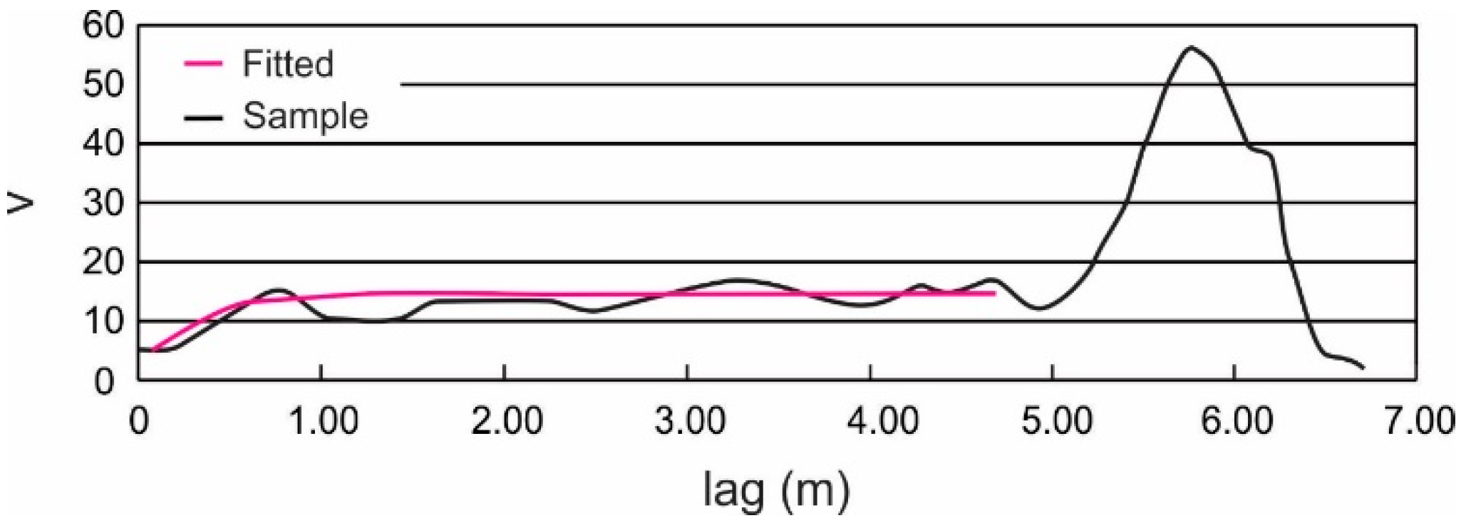
3.3.2. Estimation of θ Using the Semi-Variogram

The semi-variogram is an unbiased estimator of the variance of the differences, 0.5E[(T_ij+k − T_ij)²] [39]. It is superior to direct estimates of correlation because it does not depend on the estimated mean and is unbiased. For the i’th sample core, the sample semi-variogram is defined by;

$$\widehat{V_i}\left({\tau }_k\right)=\frac{1}{2\left(n_i-k\right)}{{\displaystyle \sum }}_{j=1}^{n_{i-k}}{\left(T_{i,j+k}-T_{ij}\right)}^2, k=0,1,\dots \dots ,n_i-1$$

(9)

In the following statistical analysis, a Markov correlation function will be assumed, having the form

$$\rho \left(\tau \right)=e^{\frac{-2\left|\tau \right|}{\theta }}$$

(10)

where τ is the separation distance between the points in question. When τ < θ, the points will be strongly correlated, and over short distances, soil properties will be more-or-less constant.

Equation (9) is a function of ${\tau }_k$, the vertical distance between T_i,j+k and T_ij where ${\tau }_k=k\Delta z$ and Δz represents the depth sampling interval. Figure 5 illustrates the sample variogram computed for a single core. The correlation function, Equation (10), is related to the semi-variogram through the relationship

$$\widehat{V_i}\left(\tau \right)={\sigma }_{T_i}^2\left(1-\rho \left(\tau \right)\right)$$

(11)

which can be used to develop a regression to determine the best fit correlation length. Specifically, the best fit correlation length for the i’th core is that value of θ_i which minimizes the following sum of squared errors,

$$e_i={\displaystyle \sum }_{k=1}^{0.7n_i}{\left\{{\widehat{V}}_i\left({\tau }_k\right)-{\widehat{\sigma }}_{T_i}^2\left(1-e^{\frac{-2\left|{\tau }_k\right|}{{\theta }_i}}\right)\right\}}^2$$

(12)

where ${\widehat{\sigma }}_{Ti}$ is the estimated standard deviation of the ith core where

$${\widehat{\sigma }}_{T_i}^2=\frac{1}{\left(n_i-1\right)}{\displaystyle \sum }_{n_i}^{j=1}{\left(T_{ij}-{\widehat{u}}_T\right)}^2$$

(13)

In Equation (12), the range over which the squared errors were computed was limited to 70% of the overall depth of the i’th core (n_i). This restriction is because the standard error of the estimator ${\widehat{V}}_i\left({\tau }_k\right)$ becomes too large when the lag exceeds about 70% of the overall depth. The error growth can be seen in Figure 5 towards the right end of the plot. Figure 5 also illustrates the fitted semi-variogram using the “best fit” correlation length obtained by minimizing Equation (12).

Based on the data from each core section, an estimated average global correlation length, $\widehat{\theta }$, was calculated according to;

$$\widehat{\theta }=\frac{1}{n_c}{\displaystyle \sum }{\theta }_i$$

(14)

where n_c is the total number of cores available in the study area. At the Scotian Slope, the average correlation length was found to be 0.95 m using the semi-variogram method. This value is in reasonably close agreement with correlation length of 0.7 found using the variance reduction method.

3.3.3. Choice of Averaging Domain

The above analyses suggest that the vertical correlation length is somewhere in the range of 0.7 to 0.95 m. The interest now is in determining the size of the averaging domain so that the variance can be properly estimated. Slope failure involves the shearing failure of the soil along a surface at some depth below the seabed. Due to lateral heterogeneities in soil properties, the failure surface will pass through weaker and stronger regions. Thus, the overall strength as “seen” by the slope is some sort of average of the soil strength over the failure domain. That is, slope failure is neither governed by the weakest extremes, nor by the strongest but by an average. The question, then, is how should this average be determined? Ideally, the area of the slope failure surface would be known, and local averaging over this area can be carried out using the correlation length in the direction of this surface and the variance function (see Equation (8)). Unfortunately, neither the area of typical undersea slope failures nor the correlation length in the direction of typical failure surfaces (which are close to horizontal) are known.

The previous subsection estimated the vertical correlation length of the Scotian Slope. It is generally believed that the correlation length in the direction of soil layering is greater than the vertical (assumed to be across soil layers) correlation length, due to the persistence of strength properties along the layers. Phoon [40] summarizes published results and suggests that the horizontal correlation length in clay ranges from about 10 to 20 times the vertical correlation length, with an average ratio of 13.3. If it is assumed that the vertical correlation length is 0.95 m, as estimated by the semi-variogram method above, then the horizontal correlation length (assumed isotropic in the plane) would be 13.3 × 0.95 = 12.6 ≅ 13 m, and this will be assumed to be a reasonable estimate of the horizontal correlation length at the site.

The next question is: What area is typically involved in an undersea slope failure? The statistics of the soil properties used to estimate the slope failure probability are determined by averaging over the slope failure area. Unfortunately, the typical extent of undersea slope failures is not well known, and what has been reported are extremely variable [1,5,6,7,11]. What this means is that the required averaging dimensions for probabilistic slope stability calculations are currently unknown.

In this study, a reasonably conservative approach is adopted. Since smaller averaging regions lead to higher variability, and thus higher failure probabilities, it is conservative to consider a failure region which is the smallest failed slope area which nevertheless poses a significant threat to any undersea operation. Purely on the basis of engineering judgement, the authors estimate this minimum failure region to have linear dimension of about 10 m.

Finally, the way the local averaging of the data is to be done must be decided. The collected data are one-dimensional samples, and so it will be conservatively assumed that the average over the failure surface can be approximated by averaging along a line along that surface. Since local averaging over 10 m with a horizontal correlation length of about 13 m leads to the same variance as averaging over 0.7 m with correlation length 0.95 m (as estimated above), we will represent the statistics of the soil properties using local averages of our vertical data over a vertical length of 0.7 m. Therefore, for a sampling interval of 0.10 m, seven (7) consecutive undrained shear strength measurements will be averaged to represent the soil properties in the “averaged” case over a 10 m failure region.

4. Slope Stability Analysis

4.1. Deterministic Slope Stability Analysis

Deterministic slope stability analyses typical employ limit equilibrium methods [21,22]. The simplest of the limit equilibrium methods is the infinite slope method, which uses force equilibrium theory to evaluate both the resisting and driving forces on an assumed sliding surface. As mentioned above, a semi-infinite slope condition is assumed where the end and side restraining conditions of the sliding mass are ignored, the failure surface is assumed planar and parallel to the slope, and only the failure surface itself is assumed to have finite area for the purposes of estimating the variance of its shear resistance. The Factor of Safety (FS) along a potential failure plane is thus the ratio of the shear strength of the soil and the driving force within the failure plane.

The FS is generally determined using either Total Stress Stability Analysis (TSSA) or Effective Stress Stability Analysis (ESSA). For TSSA, the available shear strength is equated to the undrained shear strength mobilized at the instant when failure occurs and before any significant dissipation of shearing induced porewater pressures takes place. For ESSA, the available shear strength is the drained shear strength mobilized at large strains and over time spans sufficient to allow dissipation of porewater pressures, discussed in Section 4.1.2. Both approaches are discussed next.

4.1.1. Deterministic Total Stress Stability Analysis (TSSA)

A TSSA is performed assuming an undrained in-situ condition. The FS is defined by

$$FS=\frac{2S_u}{{\gamma }_{b}z\sin \left(2\beta \right)}$$

(15)

where S_u is the undrained shear strength of the soil, β is the slope inclination, ${\gamma }_b$ is the buoyant unit weight of the soil above the potential failure plane, and z is the vertical depth from the seabed surface to the potential failure plane.

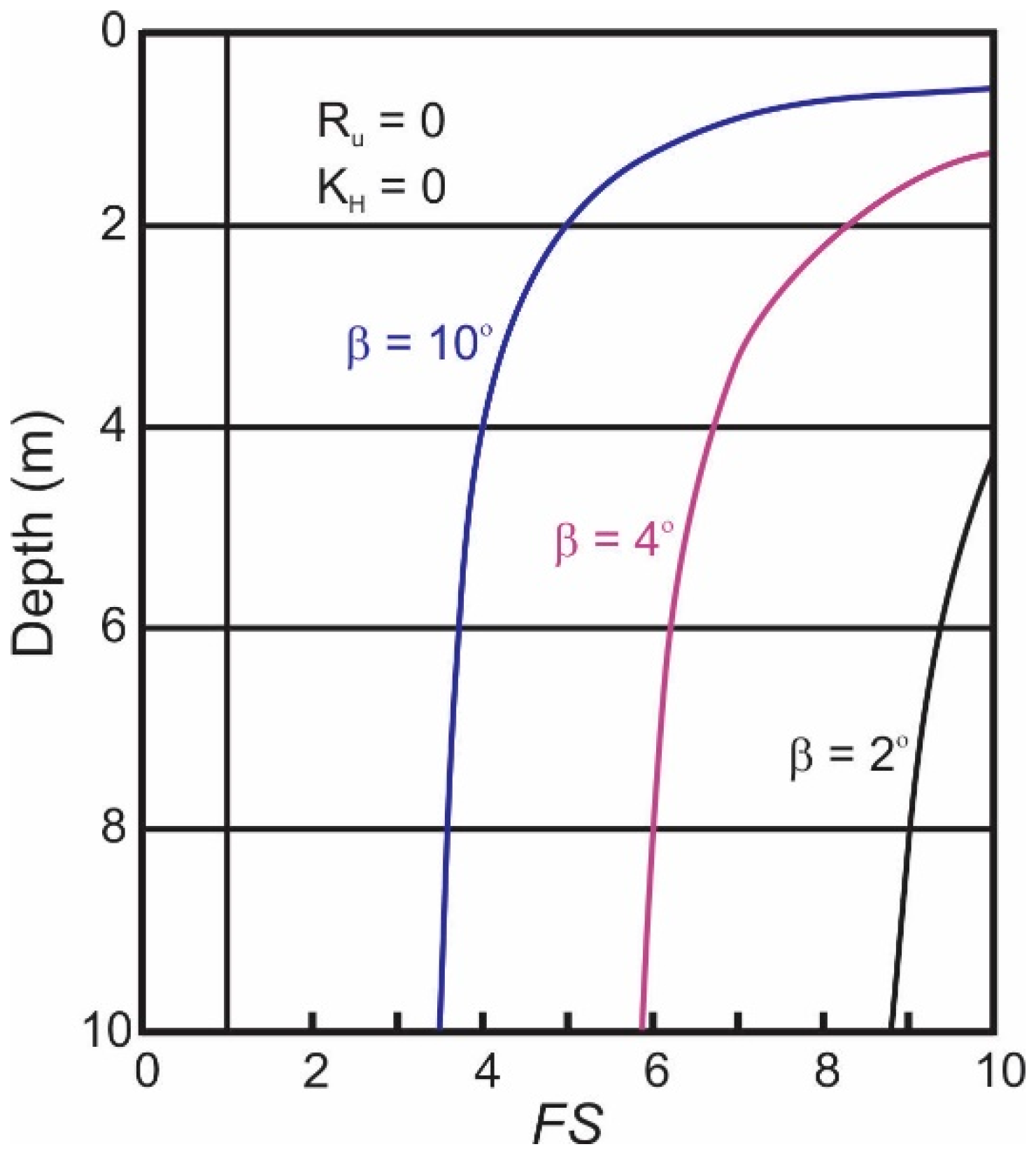
4.1.2. Deterministic Effective Stress Stability Analysis (ESSA)

An ESSA assumes fully drained conditions. The FS in this case is determined by

$$FS=\frac{2(c^{\prime }+{\gamma }_b{\cos }^2\beta \tan {\varphi }^{\prime }-U\tan {\varphi }^{\prime })}{{\gamma }_{b}z\sin \left(2\beta \right)}$$

(16)

where c’ is the apparent cohesion, ${\varphi }^{\prime }$ is the angle of internal friction, and U is the excess pore water pressure.

4.2. Probabilistic Slope Stability Analysis

The deterministic method of assessing slope stability using factor of safety is unable to explain how safe or unsafe that slope may be. The probabilistic approach allows for the estimation of the failure probability of a slope. In this paper, S_u and γ_b are assumed to be random and lognormally distributed in the TSSA approach, so that the distribution of FS in Equation (15) can be computed exactly. For the ESSA approach, the variables c’, tan φ’, and γ_b are considered to be random and a First Order Second Moment (FOSM) approach is adopted to estimate the distribution of FS in Equation (16). In the FOSM method, only the means and variances of the random variables are used to estimate the mean and variance of FS. Once the distribution of FS is known, or estimated, the slope failure probability can be computed to be the probability that FS is less than 1.0, which corresponds to the event that the slope’s shear resistance falls below the driving force.

4.2.1. Probabilistic Total Stress Stability Analysis (TSSA)

It will be assumed that the seabed inclination is known and non-random so that the distribution of the factor of safety, FS, can be determined via Equation (15) as a function of the depth to the critical failure plane, z. If the undrained shear strength, S_u, and the buoyant unit weight, γ_b, are both lognormally distributed, as assumed, then FS is also lognormally distributed and its mean and variance can be determined exactly.

If FS is lognormal, then ln(FS) is normally distribution. Taking the natural logarithm of Equation (15) gives

$$\ln \left(FS\right)=\ln \left(\frac{2S_u}{{\gamma }_{b}z\sin \left(2\beta \right)}\right)=\ln \left(S_u\right)-\ln \left({\gamma }_b\right)-\ln \left(0.5z\sin \left(2\beta \right)\right)$$

(17)

Taking expectations of both sides of Equation (17) leads to the mean of ln(FS) in terms of the means of the logarithms of the undrained shear strength and buoyant unit weight;

$$E\left[\ln FS\right]={\mu }_{\ln FS}={\mu }_{\ln S_u}-{\mu }_{\ln {\gamma }_b}-\ln \left(0.5z\sin \left(2\beta \right)\right)$$

(18)

Assuming the undrained shear strength and unit weight to be uncorrelated, which is a reasonable assumption, the variance of ln(FS) is simply the sum of the variances of ln(S_u) and ln(γ_b);

$${\sigma }_{\ln FS}^2={\sigma }_{\ln S_u}^2+{\sigma }_{\ln {\gamma }_b}^2$$

(19)

where the statistics of lnS_u are obtained from

$${\sigma }_{\ln S_u}^2=\ln \left(1+\frac{{\sigma }_{S_u}^2}{{\mu }_{S_u}^2}\right)$$

(20)

and

$${\mu }_{\ln S_u}=\ln \left({\mu }_{S_u}\right)-\frac{1}{2}{\sigma }_{\ln S_u}^2$$

(21)

and similarly for the statistics of $\ln {\gamma }_b$. The actual mean and variance of FS can be calculated using the inverse transformations;

$$u_{FS}=\exp \left({\mu }_{\ln FS}+\frac{1}{2}{\sigma }_{\ln FS}^2\right)$$

(22)

$${\sigma }_{FS}^2=u_{FS}^2\left(e^{{\sigma }_{\ln FS}^2}-1\right)$$

(23)

The probability that the factor of safety will be less than unity, i.e. that the slope fails, is computed using the cumulative standard normal distribution function, Φ(z);

$$P\left[FS<1\right]=P\left(\ln FS<0\right)=\mathsf{\Phi }\left(\frac{-{\mu }_{\ln FS}}{{\sigma }_{\ln FS}}\right)$$

(24)

4.2.2. Probabilistic Effective Stress Analysis

In the case of the ESSA, the FS is a more complex function of the random variables c’, tanφ’, and γ_b. The mean factor of safety requires computing the following expectation;

$$E\left[FS\right]=E\left[\frac{2\left(c^{\prime }+{\gamma }_{b}z{\cos }^2\beta \tan {\varphi }^{\prime }-U\tan {\varphi }^{\prime }\right)}{{\gamma }_{b}z\sin \left(2\beta \right)}\right]$$

(25)

The apparent cohesion c’, angle of internal friction, $\tan \varphi$’, and bulk density, ${\gamma }_b$ are assumed to be random variables characterized by their means and variances.

The first-order Taylor series approximation to the mean of FS is obtained by evaluating Equation (16) at the means of the random variables on the right-hand-side;

$$E\left[FS\right]=u_{FS}\approx \frac{{\mu }_{c^{\prime +{\mu }_{{\gamma }_b}a\left(z\right)\mu tan\varphi }}}{{\mu }_{{\gamma }_b}b\left(z\right)}$$

(26)

where $a\left(z\right)=z{\cos }^2\beta$, $b\left(z\right)=0.5z\sin \left(2\beta \right)$.

The variance of the FS is also estimated using a first order approximation, according to the following;

$$Var\left[FS\right]={\sigma }_{FS}^2\approx {\sigma }_{c^{\prime }}^2{\left(\frac{\partial FS}{\partial c^{\prime }}\right)}^2+{\sigma }_{\tan \varphi }^2{\left(\frac{\partial FS}{\partial \tan \varphi }\right)}^2+{\sigma }_{{\gamma }_b}^2{\left(\frac{\partial FS}{\partial {\gamma }_b}\right)}^2$$

(27)

In order to compute the probability that the FS is less than unity, the form of the distribution of the FS must be known. If we assume that FS is at least approximately lognormally distributed then Equations (20) and (21) can be used to find ${\mu }_{\ln FS}$ and ${\sigma }_{\ln FS}^2$ and then Equation (24) to find the probability of slope failure.

5. Results and Discussion

Mass transport deposits are common along the central Scotian margin; estimated to comprise nearly 50% of the sediment stratigraphy [6]. However, slope gradients are generally less than 4° and mostly less than 2° (Figure 2C). These observations suggest the need for a quantitative slope stability assessment in order to determine the relevant factors that affect slope stability. While the analyses in this study are restricted to ~12 m sub-seabed, the approach provides insight into the general effects of spatial and temporal variability on slope stability assessment. Additionally, static stability is principally a concern to the uppermost sedimentary section where consolidation effects have not yet superseded loading effects. The vast majority of the sedimentary material recovered in the cores is undrained mud of varying proportions of silt and clay [5,11,16,17]. The sequences are interpreted as largely glaciomarine sequences deposited by fine-grained turbidity currents and hemipelagic fallout. While there are lenses or thin (cm) beds of sorted sands due to turbidity currents, these intervals were not tested because of their drained conditions. There is also ice-rafted debris that adds a coarse grained component, but this material is scattered throughout the cores and rarely forms a competent bed.

Slope stability is assessed for the site using both deterministic and probabilistic methods. Two conditions are assessed for each, total stress stability analysis (TSSA) and the effective stress stability analysis (ESSA). The data available for the TSSA is extensive while that available for ESSA is limited. In all cases, data are not correlated with lithostratigraphic units, which are assumed, for the purpose of this study, to be isotropic over the entire site.

Descriptive statistics of bulk density indicate that variability is small with depth over the site and that no trend exists in the data; at least to measurement depths from the shallow piston cores. Descriptive statistics of undrained shear strength had some variability and processing of the data was used to remove trends for further statistical analysis (see Section 3). The detrended data set still exhibited variance, but the mean and variance are now independent of depth.

With the ESSA data, only six tests were available for analysis and the data set was insufficient to assess trends, although no clear trend was qualitatively evident. The analysis was completed using only the mean and standard deviation of the limited dataset.

5.1. Total Stress Stability Analysis

The factor of safety, FS, for each core and at each depth, z, is calculated using Equation (15) assuming an undrained condition (i.e., φ = 0). Using the deterministic approach, the reported FS is the minimum value found over depth for each core. FS is calculated twice for each core; first using point shear strength measurements and, second, using a “smoothed” dataset of shear strength values averaged over a 0.7 m moving window. The averaging had the effect of removing extremely low values of undrained shear strength (which would likely be average out in the downslope direction in any case), so that the (minimum) FS for the averaged data was in general higher than that found using point values.

A summary of deterministic FS results is presented in Figure 6, which illustrates that the estimated probability that the FS will be less than unity using the point data is approximately two to four percent, while the FS obtained using the averaged data always remains above 1.0. The averaged FS generally increases by more than about 30% above that obtained using point values.

Using the probabilistic approach, the mean FS is calculated for the entire site as a function of depth, using the aggregate dataset of point estimates of undrained strength for various seabed inclinations. The results are plotted in Figure 7. It suggests a critical seabed inclination of approximately ten degrees since the minimum mean FS reaches approximately 1.0 at that inclination, which means that seabeds having an angle of ten degrees have a probability of failure of about 50%.

What is revealing in Figure 7 and Equation (15) is that the FS decreases with depth. In fact, a close look at Equation (15) shows that FS is infinite when z = 0, and decreases to $2\overline{b}/\left({\gamma }_b\sin \left(2\beta \right)\right)$, on average, when z becomes very large. Equations (1) and (2) give $\overline{b}=0.93$ (for z measured in meters), and using the mean soil buoyant unit weight for ${\gamma }_b$ = 6.7 kN/m³, the limiting mean FS for the 10° slope is found to be 0.81. This means that a 10° slope will fail at some depth with probability well in excess of 50%. The 6° slope has limiting mean FS of 1.34 and so is nominally safe at all depths (i.e., having a probability of failure well below 50%). However, since S_u is random, there is still a probability of slope failure, and this probability increases with depth below seafloor, at least until a point where consolidation or soil lithification factors become dominant.

As with the deterministic assessment, the probabilistic FS is calculated first using a point estimate of variance and again using shear strength values averaged over 0.7 m vertically. It can be seen in Figure 7 that using the averaged dataset in the probabilistic analysis reduces the scatter in the data producing smoother trend lines but does not particularly influence the estimated factor of safety.

5.2. Effective Stress Stability Analysis

As noted, there was limited data for soil strength and loading conditions for ESSA. The FS is estimated using Equation (16) by assuming constant values for pore pressure while apparent cohesion, buoyant unit weight, and angle of internal friction are assumed as random variables. All three random variables are independent of depth and expected values are used for the analysis of shear strength.

Using the probabilistic approach, the FS is estimated as a function of depth for static conditions as presented in Figure 8. The minimum factor of safety at a seabed inclination of ten (10) degrees is approximately 3.5, which exceeds the calculated value for a similar analysis using TSSA.

The probability of a FS less than one was computed with depth as presented in Figure 9 for varying slope angles. At ten degrees, the curve asymptotes at less than ${10}^{-5}$, which is acceptable for offshore foundations.

6. Summary and Conclusions

There are a total of fifty one (51) piston core sites available for assessing stability of the Scotian Slope, or approximately 3.9 sites per 1000 km². These investigation sites are limited to sampling the upper ~10 meters of soil using measurements from these cores. The infinite slope method is used to assess the potential for shallow slope failures. Such assessments are useful for offshore development projects, such as those required for oil and gas exploration and exploitation in deep water.

Bulk density and peak undrained shear strength test data for each core were assessed for use in the slope stability model. The bulk density data were found to be largely independent of depth while the shear strength data exhibited a slight increase with depth. The trend with depth identified in the shear strength data was removed using a global regression equation to create a detrended dataset for use in statistical analysis.

Spatial correlation was analyzed to allow for appropriate averaging of strength data to determine factor of safety (FS) values for slope failure by minimizing the effect of extreme values. Two methods were used, variance reduction and variogram modelling. The variance reduction method gave θ = 0.7 m. The variogram modelling method was believed to be a more reliable method for this dataset, yielding an estimated correlation length of about 0.95 m. By applying the appropriate averaging interval to the point data, the effect of extreme values on factor of safety was damped out.

The infinite slope method was used to estimate factor of safety values. A deterministic model was applied to both the point and spatially averaged core sections. The results indicate the calculated factor of safety increased on average by 30% for the study area when data are averaged over 0.7 m. A probabilistic model was also applied to both the point and spatially averaged core data in order to assess the FS for each core. It was found that there is little difference in the estimated value for FS between the averaged dataset and the point estimates using probability theory. An effective stress analysis was performed for limited data using probability theory. The analysis indicates that for static conditions, the region is inherently stable.

The deterministic method gives factor of safety values, indicating whether a slope is statically safe or unsafe, but offers no further information on how safe or unsafe, as variability of data is not taken into account. The probabilistic method does consider the variability of soil properties and gives both a distribution of the factor of safety and probability of slope failure. The probabilistic assessment is evaluated exactly for the total stress stability assessment and approximated via the Taylor series for the effective stress stability analysis. Overall, the probabilistic model provides greater flexibility in making decisions in a risk-based management model. It not only answers the question, “is the region safe?”, but it also quantifies “how safe?”.

While the results of this study demonstrate that the uppermost sediments (≲10 m) west-central Scotian Slope appear to be largely statically stable given average slope angles for the region, geoscientific investigations have shown numerous examples of submarine mass failure deposits at small and large scales (i.e., tens to hundreds of meters of thickness). The ages of these sediment failures are not tightly constrained, however, there is only sparse evidence of sediment failures that might have occurred within the last 10,000 years (10 ka), suggesting modern conditions are not conducive to slope instability. Regionally, sediment failures seem to be prevalent around 130, 75, and 50 ka and are most common between 25 and 12 ka. This timing roughly correlates to episodes of glacial advances, evidenced by ice-margin wedges on the upper slope. This correlation suggests potential linkages between sediment instability and glacial advances and/or recession. Ground accelerations because of glacial rebound, direct glacial loading, and high glacial/postglacial sedimentation rates causing lithostatic loading are some potential soil conditioning or triggering factors. Increased turbidity current erosion and slope oversteepening, high volume surface and artesian groundwater flows, and dissociation of gas hydrate are other potential causative factors that may be related to glacial epochs. Other conceivable trigger mechanisms that are not necessarily related to glaciations include rare passive margin earthquakes, salt tectonics, erosional oversteepening, turbidity currents generated by shelf storms, hydrocarbon gas or other deep-seated fluid seepage, and deep seated décollement movements that cause shallow surface failures. This abundance of evidence of sediment mass failure on the slope suggests that a thorough slope stability analysis needs to account for soil pre-conditioning factors and incorporate potential for ground accelerations. Any hazard assessment must also incorporate information on recurrence frequency, which is poorly constrained at this time.

References

1. Locat, J.; Lee, H. Submarine landslides: Advances and challenges. Can. Geotech. J. 2002, 39, 193–212. [Google Scholar] [CrossRef]
2. Hühnerbach, V.; Masson, D.G. Landslides in the North Atlantic and its adjacent seas: An analysis of their morphology, setting and behavior. Mar. Geol. 2004, 213, 343–362. [Google Scholar] [CrossRef]
3. Heezen, B.C.; Ewing, M. Turbidity currents and submarine slumps, and the 1929 Grand Banks earthquake. Am. J. Sci. 1952, 250, 849–878. [Google Scholar] [CrossRef]
4. Piper, D.J.W.; Cochonat, P.; Morrison, M.L. The sequence of events around the epicentre of the 1929 Grand Banks earthquake: Initiation of the debris flows and turbidity current inferred from side-scan sonar. Sedimentology 1999, 46, 79–97. [Google Scholar] [CrossRef]
5. Schulten, I.; Mosher, D.C.; Krastel, S.; Piper, D.J.W.; Keinast, M. Surficial Sediment Failures due to the 1929 Grand Banks Earthquake, St. Pierre Slope. Subaqueous Mass Mov. Geol. Soc. Lond. Spec. Publ. 2018, 477, SP477.25. [Google Scholar] [CrossRef]
6. Mosher, D.C.; Piper, D.J.W.; Campbell, C.D.; Jenner, K.A. Near-surface geology and sediment-failure geohazards of the central scotia slope. AAPG Bullet. 2004, 88, 703–723. [Google Scholar] [CrossRef]
7. Deptuck, M.E.; Campbell, D.C. Widespread erosion and mass failure from the 51 Ma Montagnais marine bolide impact off southwestern Nova Scotia, Canada. Can. J. Earth Sci. 2012, 49, 1567–1594. [Google Scholar] [CrossRef]
8. Mosher, D.C.; Xu, Z.; Shimeld, J. The Pliocene Shelburne mass-movement and consequent tsunami, western Scotian Slope. In Submarine Mass Movements and Their Consequences IV; Mosher, D.C., Shipp, C., Moscardelli, L., Chaytor, J., Baxter, C., Lee, H., Urgeles, R., Eds.; Springer: Dordrecht, The Netherlands, 2010; Volume 28, pp. 765–776. [Google Scholar]
9. Mosher, D.C.; Moscardelli, L.; Shipp, C.; Chaytor, J.; Baxter, C.; Lee, H.; Urgeles, R. Submarine Mass Movements and Their Consequences. In Submarine Mass Movements and Their Consequences; Mosher, D.C., Shipp, C., Moscardelli, L., Chaytor, J., Baxter, C., Lee, H., Urgeles, R., Eds.; Springer: Dordrecht, The Netherlands, 2010; Volume 28, pp. 1–8. [Google Scholar]
10. Bent, A.L. A complex double-couple source mechanism for the Ms 7.2 1929 Grand Banks earthquake. Bullet. Seismol. Soc. Am. 1995, 85, 1003–1020. [Google Scholar]
11. Piper, D.J.W. The Geological Framework of Sediment Instability on the Scotian Slope: Studies to 1999; Open File 3920; Geological Survey of Canada: Ottawa, ON, Canada, 2001; p. 202. [Google Scholar]
12. Piper, D.J.W.; Sparkes, R. Proglacial sediment instability features on the Scotian slope at 63 degrees W. Mar. Geol. 1987, 76, 15–31. [Google Scholar] [CrossRef]
13. Mosher, D.C. A margin-wide BSR gas hydrate assessment: Canada’s Atlantic margin. J. Mar. Pet. Geol. 2011, 28, 1540–1553. [Google Scholar] [CrossRef]
14. Nixon, M.F.; Grozic, J.L.H. A simple model for submarine slope stability analysis with gas hydrates. Nor. J. Geol. 2006, 89, 309–316. [Google Scholar]
15. Lofi, J.; Inwood, J.; Proust, J.-N.; Monteverde, D.H.; Loggia, D.; Basile, C.; Otsuka, H.; Hayashi, T.; Stadler, S.; Mottl, M.J.; et al. Fresh-water and salt-water distribution in passive margin sediments; insights from Integrated Ocean Drilling Program Expedition 313 on the New Jersey margin. Geosphere 2013, 9, 1009–1024. [Google Scholar]
16. Campbell, D.C.; Piper, D.J.W.; Mosher, D.C.; Jenner, K.A. Surficial Geology and Sun-Illuminated Seafloor Topography, Mohican Channel, Scotian Slope, Offshore Nova Scotia; “A” Series Map 2127A; Geological Survey of Canada: Ottawa, ON, Canada, 2008; 1 sheet. [Google Scholar] [CrossRef]
17. Campbell, D.C.; Piper, D.J.W.; Mosher, D.C.; Jenner, K.A. Surficial Geology and Sun-Illuminated Seafloor Topography, Verrill Canyon, Scotian Slope, Offshore Nova Scotia; “A” Series Map 2128A; Geological Survey of Canada: Ottawa, ON, Canada, 2008; 1 sheet. [Google Scholar] [CrossRef]
18. Piper, D.J.W. Late Cenozoic evolution of the continental margin of eastern Canada. Nor. J. Geol. 2005, 85, 231–244. [Google Scholar]
19. Mosher, D.C.; Moran, K.M.; Zevenhuizen, J. Surficial Geology and Physical Properties 18: Scotian Slope: Verrill Canyon. In East Coast Basin Atlas Series: Scotian Shelf; Atlantic Geoscience Centre, Geological Survey of Canada: Dartmouth, NS, Canada, 1991; p. 145. [Google Scholar]
20. Mosher, D.C.; Moran, K.M.; Hiscott, R.N. Late Quaternary sediment, sediment mass-flow processes and slope instability on the Scotian Slope. Sedimentology 1994, 41, 1039–1061. [Google Scholar] [CrossRef]
21. Taylor, D.W. Stability of earth slopes. J. Boston Soc. Civ. Eng. 1937, 24, 197–246. [Google Scholar]
22. Bishop, A.W. The use of the slip circle in the stability analysis of slopes. Géotechnique 1955, 5, 7–17. [Google Scholar] [CrossRef]
23. Griffiths, D.V.; Huang, J.; de Wolfe, G.F. Numerical and analytical observations on long and infinite slopes. Int. J. Numer. Anal. Methods Geomech. 2011, 35, 569–585. [Google Scholar] [CrossRef]
24. Griffiths, D.V.; Huang, J.; Fenton, G.A. On the reliability of earth slopes in three dimensions. Proc. R. Soc. A 2009, 465, 3145–3164. [Google Scholar] [CrossRef] [Green Version]
25. Hicks, M.A.; Nuttal, J.D.; Chen, J. Influence of heterogeneity on 3D reliability and failure consequences. Comput. Geotech. 2014, 61, 198–208. [Google Scholar] [CrossRef]
26. Griffiths, D.V.; Huang, J.; Fenton, G.A. Probabilistic infinite slope analysis. Comput. Geotech. 2010, 38, 577–584. [Google Scholar] [CrossRef]
27. Wade, J.A.; MacLean, B.C. Chapter 5: Aspects of the Geology of the Scotian Basin from Recent Seismic and Well Data. In The Geology of the Southeastern Margin of Canada; Keen, M.J., Williams, G.L., Eds.; Geological Survey of Canada: Ottawa, ON, Canada, 1990; Volume 2, pp. 190–238. [Google Scholar] [CrossRef]
28. Swift, S.A. Late Pleistone sedimentation on the continental slope and rise off western Nova Scotia. Geol. Soc. Am. Bullet. 1985, 96, 832–841. [Google Scholar] [CrossRef]
29. Piper, D.J.W.; Normark, W.R. Late Cenozoic sea level changes and the onset of glaciation: Impact on continental slope progradation off eastern Canada. Mar. Pet. Geol. 1989, 6, 336–348. [Google Scholar] [CrossRef]
30. Mosher, D.C.; Piper, D.J.W.; Vilks, G.V.; Aksu, A.E.; Fader, G.B. Evidence for Wisconsinan glaciations in the Verrill Canyon Area, Scotian Slope. Quat. Res. 1989, 31, 27–40. [Google Scholar] [CrossRef]
31. Stea, R.R.; Piper, D.J.W.; Fader, G.B.J.; Boyd, R. Wisconsinan glacial and sea level history of maritime Canada and adjacent continental shelf: A correlation of land and sea events. Geol. Soc. Am. Bullet. 1998, 110, 821–845. [Google Scholar] [CrossRef]
32. Piper, D.J.W.; Mosher, D.C.; Newton, S. Ice-margin seismic stratigraphy of the central Scotian Slope eastern Canada. Geol. Surv. Can. Curr. Res. 2002, 2002-E16, 10. [Google Scholar]
33. Mosher, D.C.; Campbell, D.C.; Gardner, J.V.; Piper, D.J.W.; Chaytor, J.D.; Rebesco, M. The role of deep-water sedimentary processes in shaping a continental margin: The Northwest Atlantic. Mar. Geol. 2017, 392, 245–259. [Google Scholar] [CrossRef]
34. Skinner, L.C.; McCave, I.N. Analysis and modelling of gravity- and piston coring based on soil mechanics. Mar. Geol. 2003, 199, 181–204. [Google Scholar] [CrossRef]
35. Weaver, P.P.E.; Schultheiss, P.J. Current methods for obtaining, logging and splitting marine sediment cores. Mar. Geophys. Res. 1990, 12, 85–100. [Google Scholar] [CrossRef]
36. Head, K.H. Manual of Soil Laboratory Testing: Volume 3 Effective Stress Tests; Pentech Press: London, UK, 1992; p. 428. [Google Scholar]
37. Vanmarcke, E.H. Probabilistic Modeling of Soil Profiles. J. Geol. Eng. Div. 1977, 103, 1227–1246. [Google Scholar]
38. Vanmarcke, E.H. Reliability of Earth Slopes. J. Geol. Eng. Div. 1977, 103, 1247–1265. [Google Scholar]
39. Fenton, G.A. Estimation for Stochastic Soil Models. ASCE J. Geotech. Geoenviron. Eng. 1999, 125, 470–485. [Google Scholar] [CrossRef]
40. Phoon, K.K.; Kulhawy, F.H.; Grigoriu, M.D. Reliability-Based Design of Foundations for Transmission Line Structures; Report TR-105000; Electric Power Research Institute: Palo Alto, CA, USA, 1995; p. 380. [Google Scholar]
Figure 1. Study area (black rectangle) location on the Scotian Slope off eastern Canada. Nova Scotia (NS), Newfoundland and Labrador (NL), and New Brunswick (NB). North is to the top of the map.
Geosciences 09 00018 g001
Figure 2. Study area: (A) Morphology and core site locations (dots) used in this study. Red dots indicate cores from which samples were extracted for triaxial shear testing. Isobaths are in meters water depth; (B) slope gradient derived from the GEBCO 2014 grid and averaged with a circular smoothing window with a radius of 12.5 km. Note that the general gradient of this central Scotian Slope region is on the order of 1–3; and (C) surficial geology derived from cores and interpretation of geophysical records [16,17]. North is to the top in each map.
Geosciences 09 00018 g002
Figure 3. Geotechnical profile for core 20000360029PC (w = natural in-situ water content, PL = plastic limit, LL = liquid limit), as an example of the data available for each core in this study.
Geosciences 09 00018 g003
Figure 4. Aggregate of undrained shear strength for all cores used in this study. The trend line (in black) is defined by Su = 0.93z + 6.30 (R2 = 0.18).
Geosciences 09 00018 g004
Figure 5. Sample semi-variogram of the undrained shear strength for one sample core.
Geosciences 09 00018 g005
Figure 6. Percentile plot of total stress FS for all cores using the deterministic approach.
Geosciences 09 00018 g006
Figure 7. Plot of mean FS for various slope angles with depth for undrained conditions. The dashed lines are point averaged trends and the solid lines are averaged value trends.
Geosciences 09 00018 g007
Figure 8. Plot of FS for various slope angles with depth for drained conditions.
Geosciences 09 00018 g008
Figure 9. The probability of FS being less than one.
Geosciences 09 00018 g009