Abstract
This laboratory study aimed at investigating the mean and turbulent characteristics of a densely vegetated flow by testing four different submergence ratios. The channel bed was covered by a uniform array of aligned metallic cylinders modeling rigid submerged vegetation. Instantaneous velocities, acquired with a three-component acoustic Doppler velocimeter (ADV), were used to analyze the mean and turbulent flow structure. The heterogeneity of the flow field was described by the distributions of mean velocities, turbulent intensities, skewness, kurtosis, Reynolds stresses, and Eulerian integral scales. The exchange processes at the flow–vegetation interface were explored by applying the turbulence triangle technique, a far less common technique for vegetated flows based on the invariant maps of the anisotropic Reynolds stress tensor.
1. Introduction
Aquatic and riparian vegetation is a fundamental feature of riverine systems, and its presence deeply affects the hydraulic resistance, mass and momentum transport, and turbulent flow structure [1,2] with a variety of ecological and physical implications [3,4]. The presence of a submerged macro-roughness represented by a vegetative obstruction deeply alters the mean and turbulent structure of the flow with implications for mass and momentum exchange across the flow–vegetation interface. The hydrodynamic structure of the flow over a submerged canopy was investigated with reference to two main vegetation models: (1) rigid vegetation, in which the vegetative obstruction is generally represented by an array of rigid cylinders or prismatic elements [5,6,7], and (2) flexible vegetation, generally simulated by blade-shaped vegetation [8,9].
The rigid cylinder model is not able to reproduce a variety of flow-influencing mechanisms exhibited by natural vegetation, generally presenting a wide range of different biomechanical properties [10] and velocity-dependent drag characteristics [11,12]. Nevertheless, rigid cylinder models can be considered qualitatively effective for simulating the cross-section scale effects on the turbulence structure and describing morphodynamic processes of channels with vegetated floodplains [13]. Because of the practical importance of modeling turbulence in natural watercourses and coastal wetlands, an increasing interest in describing the turbulent flow structure in vegetated flows [14,15,16], highly rough beds, and obstructed flows [17] is noticeable.
The flow over rigid submerged vegetation has been widely investigated in order to assess the effects of vegetation (density and submergence) on the flow structure and the implications for the hydraulic resistance, turbulent structures, mixing processes, and sediment transport [5,6,18,19,20,21]. A distinctive feature of such vegetated shear flows is represented by the anisotropy of Reynolds stresses, which reflects, to a large extent, the presence of organized motions. Indeed, the anisotropic Reynolds stress component is the only part of the total stress responsible for the momentum transport [22], and, therefore, its study is crucial for the understanding and modeling of turbulence in vegetated flows.
The anisotropy pattern within the flow domain can be investigated using the technique of the anisotropy invariants proposed by Lumley and Newman [23]. This technique, fairly less common for the analysis of vegetated flows, allows for the characterization of the spatial distribution of the anisotropy degree and nature. Only few examples of the application of this methodology are available in the literature, and these mainly refer to numerical and experimental analyses of flows over highly rough beds [24,25].
In this study, the turbulent structure of the flow over a submerged array of rigid cylinders was experimentally investigated by coupling the traditional approach based on the spatial distributions of velocity statistics and spectral analysis [5,6,26] with a new methodology adopted for providing the overall description of the turbulence anisotropy, represented by the turbulence triangles [27]. Specifically, the effects of the variability of the submergence, that is, the ratio between the uniform flow depth and the cylinder’s height, on the mean velocity profiles, the distributions of higher-order velocity statistics, quadrant analysis, and the distribution of integral time and length scales were analyzed with reference to the anisotropy pattern resulting from the invariant maps.
2. Materials and Methods
2.1. Laboratory Flume
The experiments were carried out in an 8 m long, 0.4 m wide, and 0.4 m high Plexiglas-walled recirculating flume in the Laboratory of Hydraulics and Hydraulic Structures at the University of Naples Federico II (Figure 1a). The channel was supplied by a 4.5 m3 tank into which water was led through the water supply system of the laboratory from a water tower. Specifically, in order to stabilize flow rates in the channel, water was not directly pumped into the flume but, from the recirculating system reservoir, was led to a water tower with a pumping station.
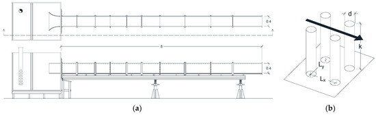
Figure 1.
(a) Experimental facility. The laboratory flume was 8 m long with a 0.4 m wide and 0.4 m deep rectangular cross-section. The bed of the flume was uniformly covered by an array of rigid cylinders. (b) Geometry of the array of aligned cylinders and specification of diameter (d), spacing ( and ), and cylinder height (k).
The discharge was measured by a magnetic flow meter (to an accuracy of ±0.1 L/s) installed on the feeding pipeline of the channel. The discharge ranged up to 30 L/s. The channel slope was set to 1%. At the inlet section, a parabolic transition from the feeding tank to the experimental channel was placed in order to reduce the disturbance at the inlet and to damp the related turbulence.
All the tests were carried out under uniform flow conditions with different cylinder submergences. In the range of considered flow rates, a uniform flow reach was identified by analyzing the backwater profiles, experimentally determined using a gauging needle (with an accuracy of 0.1 mm). For all the test runs, uniform flow conditions were observed to be restored at approximately 4.5 m from the outlet section. Measurements were taken at 2.5 m from the channel inlet, within the uniform flow section of the flume and sufficiently downstream from the inlet.
2.2. Rigid Vegetation Model
This experimental study was performed by considering a uniformly vegetated channel bed in which metallic cylinders were used to simulate rigid, submerged vegetation (Figure 1b). The 45 mm long rods of 4 mm diameter, installed in holes bored into the Plexiglas bed panels, were arranged in an aligned pattern with a constant density all over the channel bed. The spacing between cylinders, in the streamwise and spanwise directions, was equal to 25 mm (Figure 1b). Consequently, the number of cylinders per unit bed area was equal to 1600 m−2. The vegetation density was described by three other parameters:
- the frontal area per canopy volume , equal to 6.4 m−1;
- the frontal area per bed area , also known as the density roughness, computable as for vertically uniform vegetation, and equal to 0.288;
- the solid volume fraction occupied by the canopy elements , evaluable as for cylindrical elements and equal to 0.020.
The considered vegetation geometry and density, typical of dense canopies [28], were comparable to those commonly exhibited by aquatic submerged vegetation, as reported in Table 1.

Table 1.
Comparison between the current vegetation model and aquatic vegetation (from [28]).
2.3. Test Cases and Velocity Measurements
The effects of the submergence ratio on the flow structure were experimentally investigated for the hydraulic conditions reported in Table 2. Specifically, four different submergence ratios were considered: 2.4, 2.8, 3.1, and 3.4. For each condition, the canopy edge velocity (), the measured friction velocity at the canopy edge ( = ), and the bulk velocity ( = ) were evaluated. Furthermore, the relevant Reynolds numbers (the roughness = , flow = , and vegetation element = ), and the flow Froude number are indicated (Table 2).
Table 2.
Details of experimental conditions.
Under the considered conditions of shallow submerged canopies [28,29], with < 5, both turbulent stress and potential gradients drive the flow within the canopy [30].
Instantaneous velocity measurements were performed with a SonTek 16 MHz MicroADV (SonTek, San Diego, CA, USA), a three-axis acoustic Doppler velocimeter (ADV) with a down-looking probe. In order to describe the turbulence structure within and above the canopy, the maximum available sampling frequency of the instrument was adopted, that is, 50 Hz. In order to achieve well-converging higher-order moments, a sample size of more than 50,000 values was assumed [31].
ADV data were filtered by assuming a threshold correlation and signal-to-noise-ratio level of 70% and 30 dB, respectively. Finally, data were de-spiked using the phase-space threshold method [32] as modified by Wahl [33]. Velocity measurements were performed in the uniform flow reach, along a vertical line in the channel midline (Figure 2a,b). The sampling volume (SV) was approximately cylindrical with a 4 mm diameter and 4.5 mm height (Figure 2a); therefore, the distances between each acquisition point were selected to be equal to 10 mm, in order to avoid overlapping the SVs of each measurement point.
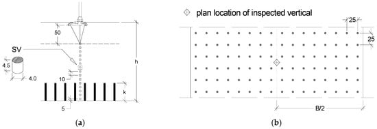
Figure 2.
(a) Position of measurement stations and geometry of sampling volume. (b) Location of inspected vertical within the cylinder array.
Considering the distance between the center of the SV and the acoustic transmitter of the probe (50 mm), the flow was investigated up to 50 mm from the water surface (Figure 2a). The orientation of the probe was defined to identify the streamwise axis of the channel with the x-axis of the probe; y is the spanwise direction (positive leftwards), and z is the vertical direction (positive upwards). The good alignment and the verticality of the instrument were addressed with a laser cross-level and a three-dimensional (3D) bubble level.
3. Results and Discussion
3.1. Mean Velocity Profiles
In Figure 3, the mean velocity profiles of , , and (for , , and directions, respectively) are shown. The velocity and distance from the bed were made dimensionless with the streamwise mean velocity at the canopy top and the vegetation height, respectively.
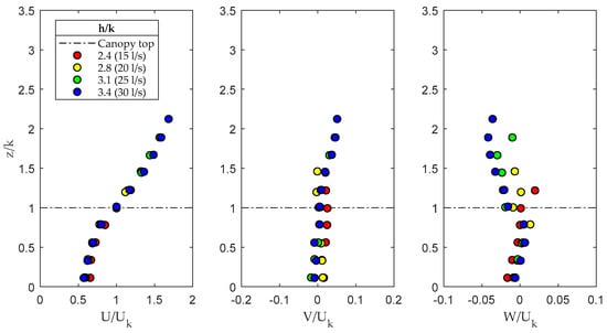
Figure 3.
Dimensionless mean velocity profiles for U, V, and W. Dash-dotted line indicates the canopy top.
The selected scaling velocity parameters and the resulting velocity profiles shown in Figure 3 were consistent with the results of previous studies [5,6,34,35]. The discontinuity in drag at the vegetation top modified the longitudinal velocity profile, characterized by an inflection point at the top of the canopy, resembling a canonical mixing layer [28]. Specifically, the drag exerted by the canopy decelerated the flow in the vegetated layer; as firstly addressed by Raupach et al. [34], this effect dominates the transfer of momentum across the flow–vegetation interface. This effect, slightly more pronounced for higher values of , is characteristic of dense canopies and, specifically, canopies with [28]. The large interfacial coherent structures, also called canopy-scale vortices, occupy the surface layer and partly penetrate the vegetation layer, depending on the canopy density. Nepf et al. [35] defined a parameter describing the scaling for the penetration depth ():
where is the drag coefficient of vegetation elements. In this study, for = 1, varied between 27 and 45 mm and / varied between 0.6 and 1.
The turbulent flow in the investigated region of the channel was fully developed, and, considering that the leading edge of the canopy was located approximately 2.5 m upstream from the measurement section, the canopy-scale vortices and the penetration depth reached a stable condition.
3.2. Turbulent Intensities
In Figure 4, the turbulent intensities in the three directions, defined as the root-mean-square values for the three velocity components, made dimensionless with the measured friction velocity at the canopy top, are shown.
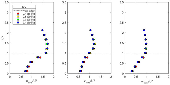
Figure 4.
Turbulent intensities in the three directions x, y, and z.
The profiles showed a similar trend, collapsing together along the same curve. The maximum longitudinal turbulent intensities occurred at the top and directly above the canopy. The turbulent intensity decreased within the vegetation layer and towards the free surface. Indeed, the vegetation damped the turbulence, and this effect was observed to be slightly more pronounced for higher submergence ratios. At the canopy top, the normalized vertical fluctuating velocity component was ≈1 for each submergence. For dense canopies, the characteristic value is about 1.1, which is typical for mixing layers, in agreement with Raupach et al. [34] and Poggi et al. [5]. Larger values, up to 1.3, are typical for sparse canopies. At the canopy top, the normalized streamwise and vertical fluctuating velocity components attained values in agreement with Raupach et al. [34], Poggi et al. [5], and Nezu et al. [6] for dense canopies.
3.3. Skewness and Kurtosis
The skewness of the velocity fluctuations is shown in Figure 5. A non-zero skewness indicates an asymmetric probability density function of the considered variable, which means that larger excursions in one direction were more probable than in the other direction, depending on the sign of the statistics. The profiles of Figure 5 describe a clear trend for the skewness in to take positive values inside the canopy and negative values outside and, complementarily, for the skewness in to take negative values inside the canopy and positive values outside. This trend indicates the dominant role of sweep events inside the cylinder array and the ejection events above the canopy, in agreement with the results of other experimental analyses [5,6,14]. The intensity of these effects, as confirmed by quadrant analysis, increased with the submergence ratio because of the increasing momentum transfer between the vegetated and non-vegetated zones. A normal distribution could be assumed for the fluctuations in the spanwise direction.
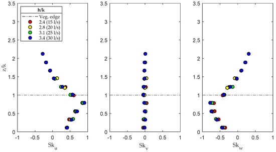
Figure 5.
Skewness of the fluctuation velocity components in the three directions x, y, and z.
The kurtosis profiles evaluated for the three velocity fluctuation components, shown in Figure 6, consistent with the results of Poggi et al. [5] for dense canopies, tended to assume higher values in the regions immediately around the canopy top. This effect, as confirmed by the quadrant analysis illustrated in the next section, confirmed the dominant role of sweep and ejection events for the Reynolds shear-stress production and the momentum transport at the canopy top.
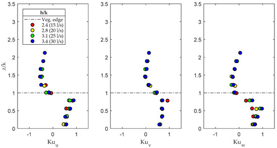
Figure 6.
Kurtosis of the fluctuation velocity components in the three directions x, y, and z.
Within the canopy, was observed to attain values of >1, consistent with the lateral fluctuations related to the von Karman vortex shedding process induced by the presence of cylinders.
3.4. Reynolds Shear Stress
In Figure 7, the Reynolds shear stresses −, normalized by the squared friction velocity at the canopy top, are plotted along the inspected vertical for the four different submergences. The Reynolds stress profile attained a peak at the canopy top () and exhibited a sharp decrease within the canopy. This effect, as observed by other authors [6,30], was due to the presence of the canopy elements, which inhibited the momentum transfer between the surface layer and the underlying vegetated layer.
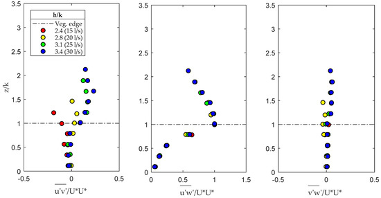
Figure 7.
Reynolds stress profiles. The quantities are normalized with square of the friction velocity at the canopy top .
The penetration depth (Table 3), estimated as the elevation at which the Reynolds stress decays to 10% of its maximum value [30], was evaluated from Figure 7 for the different submergence ratios, showing a good agreement with the estimation of the scaling of Equation 1. Depending only on the vegetation density, approximately constant values were observed for all the test runs.
Table 3.
Penetration depth.
As the submergence increased, the shape of the normalized xy shear-stress profile changed, exhibiting higher values. These effects were ascribable to the growing effects of the secondary currents inside the experimental channel [6], considering that the aspect ratio of the channel (/( − )) ranged from 3.8 to 6.2.
3.5. Quadrant Analysis
The trend emerging from the skewness and kurtosis distributions was confirmed by the results of the quadrant analysis. This simple conditional-sampling technique can provide useful information for the interpretation and the detection of organized coherent structures in the flow, allowing the nature of contributions to the Reynolds stress from the different events to be understood [36]. In quadrant analysis [36,37,38], the velocity fluctuation components are plotted on a plane. The plane is divided into four quadrants; each one is characteristic of a different event:
- quadrant 1: outward interaction ( > , > );
- quadrant 2: ejection ( < , > );
- quadrant 3: inward interaction ( < , < );
- quadrant 4: sweep ( > , < ).
In order to highlight the contribution of extreme events to the overall Reynolds stress, a hyperbolic threshold was introduced, given by the expression [5,6,36], which defines, on the plane, a hyperbolic hole; the parameter , the size of the hole, was assumed to be equal to 2 [36]. At any point in the flow domain, the total contribution of each quadrant to the Reynolds stress can be calculated as follows [18]:
where the subscript refers to the i quadrant and is a dummy variable equal to 1 if belongs to the ith quadrant and equal to 0 otherwise. Clearly, .
The contribution of the extreme events of each quadrant, instead, can be calculated as follows [36]:
where is the threshold level defining the size of the hyperbolic hole region and the subscript refers to the i quadrant. is a dummy variable equal to 1 if belongs to the ith quadrant and and equal to 0 otherwise.
In Figure 8, the contribution of each quadrant to the Reynolds stress is plotted as a function of the normalized distance from the bed. The contributions of the different events were firstly evaluated considering equal to 0 and secondly by considering equal to 2 (Figure 8), to make more evident the role played by sweep and ejection events in the Reynolds stress production.
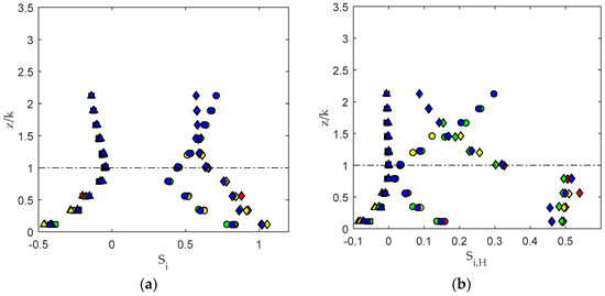
Figure 8.
Contribution of each quadrant to the overall Reynolds stress: (a) evaluated with Equation (2) considering all the events, and (b) evaluated with Equation (3) considering only the extreme events, assuming the parameter equal to 2. Inward and outward interactions are represented by solid squares (■) and triangles (▲), respectively, and sweep and ejection interactions by diamonds (♦) and circles (●). The different colors refer to the four different considered conditions: blue: 30 L/s; green: 25 L/s; yellow: 20 L/s; red: 15 L/s.
The quadrant analysis confirmed the central role of sweep within the canopy and, complementarily, the dominant role of ejection events in the region above the canopy, only slightly affected by the submergence. Inward and outward interaction event contributions were almost equal and negligible. At , the contributions of sweep and ejection were approximately equal.
3.6. Turbulence Anisotropy
In order to provide an overall description of turbulence in the flow over the rigid vegetated bed, mean time invariant analyses were performed using the turbulence triangle [23,27], an anisotropy-invariant map. The anisotropy of turbulence is described by the Reynolds stress anisotropy tensor:
The non-dimensional form of the anisotropy tensor, recognized in the trace of the Reynolds stress tensor as twice the turbulence kinetic energy (), is given by
The invariants of can quantify the different states of turbulence and the relative strength of the fluctuating velocity components, that is, the componentality of the turbulence field [39].
Anisotropy-invariant maps are two-dimensional (2D) domains based on invariant properties of . Specifically, in the turbulence triangles, the axis variables are linear combinations of the Reynolds stress anisotropy eigenvalues ; the map defines the domain of all possible turbulent flows. Each boundary of the map is characteristic of a particular turbulence state (vertices are related to one-dimensional (1D), 2D, and 3D turbulence; edges are related to specific turbulent processes: axisymmetric expansion, axisymmetric contraction, and two-component turbulence). More details on linear and non-linear invariable maps and the shape and meaning of boundaries can be found in [40].
In Figure 9, the structure of the flow over the rigid vegetated bed is described through a turbulence triangle. Each point has coordinates and [40], where and are the quadratic and cubic invariants of the Reynolds stress anisotropic tensor, respectively.
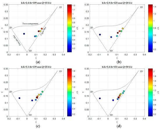
Figure 9.
Invariant maps for turbulence componentality analysis for the different submergences: (a) 2.4; (b) 2.8; (c) 3.1; (d) 3.4.
The patterns defined by the points of the invariant map, in the range of the considered Reynolds numbers and submergences, were clear and approximately equal for all the considered conditions.
Moving from the bed toward the water surface, the points of the invariants of the Reynolds stress tensor described a peculiar path. Near the channel bed, at approximately equal to 0.1, the turbulence approached a 2D state. Moving upwards, the turbulence reached, at the top of the canopy (), a quasi-1D state: the fluctuation in the streamwise direction was dominant because of the presence of the large-scale coherent structures, and the shape of the turbulence was cigar-like. Specifically, for all the investigated conditions, the 1D characteristic and the degree of anisotropy were maximums at z/k = 1. Above the canopy (), the path described by the points of the invariants moved through the axisymmetric expansion tending to an isotropic state. Because of the dimension of the ADV SV, for each submergence, the last measurement point was 5 cm from the surface (for the highest flow condition, the last point was at equal to 2.1; the water surface was at equal to 3.4); therefore, the evolution of the path to the water surface is not shown. Nevertheless, because of the presence of the water surface, which inhibits the vertical fluctuations, the turbulence structure was expected to become 2D [25].
The 2D state of the turbulence inside the canopy, and, specifically, in the lower part of the vegetated layer, indicated the growing importance of the lateral fluctuations due to the von Karman vortex shedding process triggered by the cylinder array, as shown also by the plots of Figure 6. The onset of this process was ensured by the local high stem Reynolds number ≈ 850 > 150–200 [41].
In Figure 10, the dimensionless power density spectra of the lateral velocity fluctuations, evaluated at = 0.1 for all the investigated conditions, are shown together. The spectral density was normalized by dividing by the product of the root-mean-square level of the local longitudinal velocity and the stem diameter. The frequency is given in terms of Strouhal number ( = ). A concentration of energy in the range of the Strouhal number between 0.2 and 0.1 was observed, in agreement with the frequency of the vortex shedding process observed by Poggi et al. [5] and Zong et al. [42] for cylinder arrays. The von Karman vortex shedding peak in the power density spectra was only slightly visible because of the deep penetration of the canopy-scale structures within the array (Table 3).
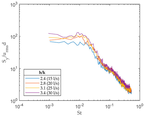
Figure 10.
Power density spectra at = 5 mm for the different runs. The ordinates were made dimensionless by dividing by the local root mean square multiplied by the diameter of the rods.
In order to highlight the effects of the rigid cylinders on the turbulent structure, a comparison between the anisotropy-invariant maps of the vegetated bed (i.e., Figure 9d) and the correspondent maps from LES applied to an open channel flow over a smooth bed at = 13,680 [25] is shown in Figure 11.
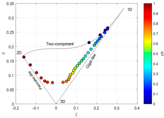
Figure 11.
Turbulence triangle for the smooth bed case (Reh = 13,680) (from [25]).
Although the two plots refer to flows with different Reynolds numbers (13,680 and 75,000 for the smooth and uniformly vegetated beds, respectively), the comparison allows the main differences in terms of the turbulence anisotropy pattern to be seen. While in the viscous sublayer, directly above the flume bed, a two-component isotropic turbulence was expected for both the conditions; at / = 0.1 (/ ≈ 0.04) the behavior was different and the turbulence in the vegetated case presented a 2D structure. On the contrary, in the smooth bed, as expected for a canonical boundary layer, the turbulence was highly anisotropic and 1D. Moving upwards, the evolution of the pattern was still different, and, while for the vegetated bed the anisotropy progressively increased and a 1D characteristic was observed, for the smooth bed, the turbulence gradually returned to isotropy via an axisymmetric expansion process. For the vegetated bed, turbulence at / ≈ 2 (/ ≈ 0.6) still presented a high degree of anisotropy and a cigar-like shape, because this area of the flow was dominated by the canopy-scale coherent structures. For the smooth bed, the turbulence became quasi-isotropic at / ≈ 0.7 and then presented, approaching the free surface, a tendency toward a 2D structure.
3.7. Integral Scales
In order to investigate the time and spatial extent of the coherent structures dominating the flow, the calculation of Eulerian integral scales was performed. Specifically, an integral time scale is a measure of the memory effect in the flow field of the persistence of a large-scale eddy at a fixed Eulerian point. In Figure 12a, integral time scales evaluated by means of Equation (6) for the three directions along the inspected vertical and for the different considered conditions are shown.
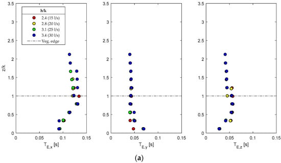
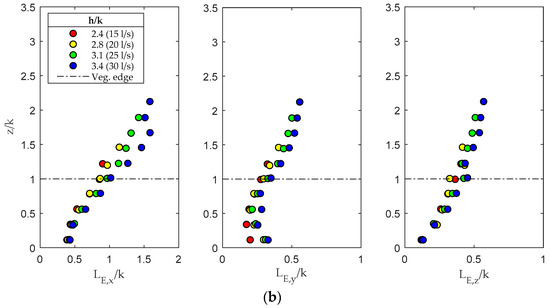
Figure 12.
Profiles of integral scales of the flow: (a) Eulerian integral time scales; (b) Eulerian integral length scales.
The integration domain for the determination of the integral time scale ranged from zero up to the value at which the autocorrelation function fell to 1/e [43,44] so as to define an integration domain independent of the shape of the autocorrelation function [45]. Large eddies persist for a long time and are advected slowly; thus the integral scale was large.
The Eulerian integral length scales could be estimated from the single-point integral time scales by applying Taylor’s frozen-turbulence hypothesis and assuming the mean local longitudinal velocity as the convection velocity of the mean eddies using the equation .
The integral length scales evaluated for the four different conditions are shown in Figure 12b. The results confirmed the interpretation of the flow structure drawn from the anisotropy analysis.
The turbulence exhibited a quasi-2D structure near the channel bed, within the vegetation layer, as a result of the dominant effects of the stem-scale turbulence and von Karman vortices. Moving toward the vegetation top, while tended to decrease, and showed a progressively increasing trend, confirming the axisymmetric expansion process shown by the invariant maps. Specifically, at the canopy top, and were approximately equal to and 0.4 showing that, in the upper vegetated layer, the dominant eddy size was in the order of , consistent with the results of Raupach et al. [34] and Nezu et al. [6]. Over the canopy, the three integral length scales became larger; in this region the flow was dominated by the canopy-scale turbulence.
In Figure 13, the good fit between the integral length scales relative to runs 3 and 4 and the results of Nezu et al. for dense canopies [6] are shown.
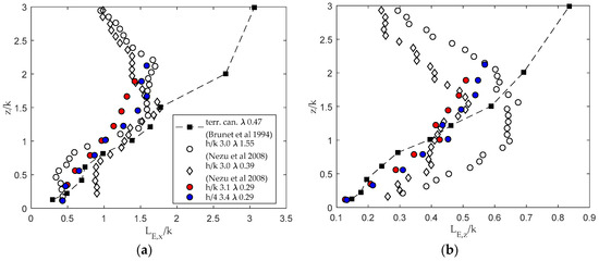
Figure 13.
Comparison with analogous literature calculation of integral length scales [6,46]: (a) integral length scale profile along the vertical direction for the x component; (b) integral length scale profile along the vertical direction for the z component. In the plot, only the profiles evaluated for the two highest submergence conditions are reported.
In comparison with terrestrial canopy, aquatic canopy is depressed by the free surface, while, on the contrary, terrestrial canopy is unconfined. This result confirms how, in aquatic canopy, eddies may be influenced by the submergence.
4. Conclusions
The results of this experimental analysis provided an exhaustive picture of the effects of increasing submergence on the mean and turbulent structure of the flow over an array of submerged rigid cylinders modeling dense vegetation. Specifically, rigid cylinders were arranged in an aligned pattern, modeling submerged rigid vegetation. Different submergence ratios were investigated.
A variation of approximately 50% of / was observed not to significantly affect the flow structure, indicating that, in the range of the tested submergences, the stem density played a major role in the hydrodynamic structure of the flow, as reported by Nezu et al. and Poggi et al. [5,6].
The mean velocity profiles presented a characteristic inflected shape because of the different flow velocities within and above the vegetation; this was slightly more pronounced for the higher values of submergence. This effect, related to the high density of the cylinder array, was the main feature of the considered obstructed flow, and the consequent Kelvin–Helmholtz-type instability dominated the momentum exchange across the vegetated interface.
The higher-order moments and the quadrant analysis allowed the Reynolds stress production process and distribution throughout the water depth to be characterized, confirming the dominant role of sweep and ejection bursting events. The maximum Reynolds stress was observed at the top of the canopy. A sudden decay of within the vegetation, due to the significant contribution of the drag force to the momentum balance, was observed. The integral length scales showed a trend characteristic of dense aquatic canopy, allowing eddies of the flow field to be characterized.
The invariant maps, generally used for verification of numerical model results and here applied for the interpretation of the componentality of the turbulence in the vegetated flow, gave very interesting results, showing their usefulness in interpreting the turbulent structure of vegetated flows. In particular, the flow structure picture emerging from the anisotropy analysis was consistent with the traditional statistical analysis of turbulence, providing a complete description of the flow field. Specifically, the method can be easily transferred to more complex vegetation models and configurations and, together with traditional analysis, can contribute to the understanding of turbulence in vegetated contexts.
Author Contributions
Conceptualization and methodology, G.C. and P.G.; Formal analysis and investigation, G.C.; Writing—Original Draft, G.C.; Writing—Review & Editing, P.G., N.F. and M.G. All authors read and approved the final manuscript.
Funding
This research received no external funding.
Acknowledgments
The authors acknowledge the two anonymous reviewers for their constructive comments which helped to improve the paper.
Conflicts of Interest
The authors declare no conflict of interest.
References
- Järvelä, J.; Aberle, J.; Dittrich, A. Flow-vegetation-sediment interaction: Research challenges. In River Flow 2006, Proceedings of the 2006-Third International Conference Fluvial Hydraul, Lisbon, Portugal, 6–8 September 2006; Taylor & Francis: New York, NY, USA, 2006; pp. 2017–2026. [Google Scholar]
- Nepf, H.M. Flow and transport in regions with aquatic vegetation. Annu. Rev. Fluid Mech. 2012, 44, 123–142. [Google Scholar] [CrossRef]
- Tabacchi, E.; Lambs, L.; Guilloy, H. Impacts of riparian vegetation. Hydrol. Process. 2000, 14, 2959–2976. [Google Scholar] [CrossRef]
- Gurnell, A. Plants as river system engineers. Earth Surf. Process. Landf. 2013, 40, 135–137. [Google Scholar] [CrossRef]
- Poggi, D.; Porporato, A.; Ridolfi, L.; Albertson, J.D.; Katul, G.G. The effect of vegetation density on canopy sub-layer turbulence. Boundary-Layer Meteorol. 2004, 111, 565–587. [Google Scholar] [CrossRef]
- Nezu, I.; Sanjou, M. Turburence structure and coherent motion in vegetated canopy open-channel flows. J. Hydro-Environ. Res. 2008, 2, 62–90. [Google Scholar] [CrossRef]
- Rowiński, P.M.; Kubrak, J. A mixing-length model for predicting vertical velocity distribution in flows through emergent vegetation. Hydrol. Sci. J. 2002, 47, 893–904. [Google Scholar] [CrossRef]
- Ghisalberti, M.; Nepf, H.M. Mixing layers and coherent structures in vegetated aquatic flows. J. Geophys. Res. 2002, 107, 1–11. [Google Scholar] [CrossRef]
- Sukhodolova, T.A.; Sukhodolov, A.N. Vegetated mixing layer around a finite-size patch of submerged plants: Part 1. Theory and field experiments. Water Resour. Res. 2012, 48, 1–16. [Google Scholar] [CrossRef]
- Aberle, J.; Järvelä, J. Flow resistance of emergent rigid and flexible floodplain vegetation. J. Hydraul. Res. 2013, 51, 33–45. [Google Scholar] [CrossRef]
- Västilä, K.; Järvelä, J. Modeling the flow resistance of woody vegetation using physically based properties of the foliage and stem. Water Resour. Res. 2014, 50, 229–245. [Google Scholar] [CrossRef]
- Caroppi, G.; Västilä, K.; Järvelä, J.; Rowiński, P.M. Experimental investigation of turbulent flow structure in a partially vegetated channel with natural-like flexible plant stands. In New Challenges in Hydraulic Reseearch and Engineering, Proceedings of the 5th IAHR Europe Congress, Trento, Italy, 12–14 June 2018; Armanini, A., Nucci, E., Eds.; Taylor & Francis: New York, NY, USA, 2018; pp. 615–616. [Google Scholar]
- Vargas-Luna, A.; Crosato, A.; Calvani, G.; Uijttewaal, W.S.J. Representing plants as rigid cylinders in experiments and models. Adv. Water Resour. 2016, 93, 205–222. [Google Scholar] [CrossRef]
- Devi, T.B.; Kumar, B. Experimentation on submerged flow over flexible vegetation patches with downward seepage. Ecol. Eng. 2016, 91, 158–168. [Google Scholar] [CrossRef]
- Peruzzo, P.; de Serio, F.; Defina, A.; Mossa, M. Wave height attenuation and flow resistance due to emergent or near-emergent vegetation. Water 2018, 10, 402. [Google Scholar] [CrossRef]
- Viero, D.P.; Pradella, I.; Defina, A. Free surface waves induced by vortex shedding in cylinder arrays. J. Hydraul. Res. 2017, 55, 16–26. [Google Scholar] [CrossRef]
- Coscarella, F.; Servidio, S.; Ferraro, D.; Carbone, V.; Gaudio, R. Turbulent energy dissipation rate in a tilting flume with a highly rough bed. Phys. Fluids 2017, 29, 085101. [Google Scholar] [CrossRef]
- Raupach, M.R.; Thom, A.S. Turbulence in and above Plant Canopies. Annu. Rev. Fluid Mech. 1981, 13, 97–129. [Google Scholar] [CrossRef]
- Ghannam, K.; Poggi, D.; Porporato, A.; Katul, G.G. The Spatio-temporal Statistical Structure and Ergodic Behaviour of Scalar Turbulence Within a Rod Canopy. Boundary-Layer Meteorol. 2015, 157, 447–460. [Google Scholar] [CrossRef]
- Gualtieri, P.; De Felice, S.; Pasquino, V.; Doria, G.P. Use of conventional flow resistance equations and a model for the Nikuradse roughness in vegetated flows at high submergence. J. Hydrol. Hydromech. 2018, 66, 107–120. [Google Scholar] [CrossRef]
- Ghannam, K.; Katul, G.G.; Bou-Zeid, E.; Gerken, T.; Chamecki, M. Scaling and similarity of the anisotropic coherent eddies in near-surface atmospheric turbulence. J. Atmos. Sci. 2018, 75, 943–964. [Google Scholar] [CrossRef]
- Pope, S.B. Turbulent Flows; Cambridge University Press: Cambridge, UK, 2000; pp. 88–89. [Google Scholar]
- Lumley, J.L.; Newman, G.R. The return to isotropy of homogeneous turbulence. J. Fluid Mech. 1977, 82, 161–178. [Google Scholar] [CrossRef]
- Smalley, R.; Leonardi, S.; Antonia, R.A.; Djenidi, L.; Orlandi, P. Reynolds stress anisotropy of turbulent rough wall layers. Exp. Fluids 2002, 33, 31–37. [Google Scholar] [CrossRef]
- Bomminayuni, S.; Stoesser, T. Turbulence statistics in an open-channel flow over a rough bed. J. Hydraul. Eng. 2011, 137, 1347–1358. [Google Scholar] [CrossRef]
- Ghisalberti, M.; Nepf, H.M. The structure of the shear layer in flows over rigid and flexible canopies. Environ. Fluid Mech. 2006, 6, 277–301. [Google Scholar] [CrossRef]
- Choi, K.S.; Lumley, J.L. The return to isotropy of homogeneous turbulence. J. Fluid Mech. 2001, 436, 161. [Google Scholar] [CrossRef]
- Nepf, H.M. Hydrodynamics of vegetated channels. J. Hydraul. Res. 2012, 50, 262–279. [Google Scholar] [CrossRef]
- Augustijn, D.C.M.; Huthoff, F.; Van Velzen, E.H. Comparison of vegetation roughness descriptions. In Proceedings of the Fourth International Conference Fluvial Hydraul, River Flow 2008, Cesme, Turkey, 3–5 September 2008; p. 9. [Google Scholar]
- Nepf, H.M.; Vivoni, E.R. Flow structure in depth-Iimited, vegetated flow. J. Geophys. Res. 2000, 105, 28547–28557. [Google Scholar] [CrossRef]
- Doroudian, B.; Hurther, D.; Lemmin, U. Discussion of “Turbulence measurements with acoustic doppler velocimeters” by Carlos M. Garcia, Mariano I. Cantero, Yarko Nino, and Marcelo H. Garcia. J. Hydraul. Eng. 2007, 133, 1283–1288. [Google Scholar] [CrossRef]
- Goring, D.G.; Nikora, V.I. Despiking acoustic doppler velocimeter data. J. Hydraul. Eng. 2002, 128, 117–126. [Google Scholar] [CrossRef]
- Wahl, T.L. Discussion of “Despiking acoustic doppler velocimeter data” by Derek G. Goring and Vladimir I. Nikora January. J. Eng. Mech. 2003, 128, 2002–2003. [Google Scholar]
- Raupach, M.R.; Finnigan, J.J.; Brunei, Y. Coherent eddies and turbulence in vegetation canopies: The mixing-layer analogy. Boundary-Layer Meteorol. 1996, 78, 351–382. [Google Scholar] [CrossRef]
- Nepf, H.M.; Ghisalberti, M.; White, B.L.; Murphy, E. Retention time and dispersion associated with submerged aquatic canopies. Water Resour. Res. 2007, 43, 1–10. [Google Scholar] [CrossRef]
- Lu, S.S.; Willmarth, W.W. Measurements of the structure of the Reynolds stress in a turbulent boundary layer. J. Fluid Mech. 1973, 60, 481–511. [Google Scholar] [CrossRef]
- Wallace, J.M.; Brodkey, R.S. Reynolds stress and joint probability density distributions in the u-v plane of a turbulent channel flow. Phys. Fluids 1977, 20, 351–355. [Google Scholar] [CrossRef]
- Nakagawa, H.; Nezu, I. Prediction of the contributions to the Reynolds stress from bursting events in open-channel flows. J. Fluid Mech. 1977, 80, 99. [Google Scholar] [CrossRef]
- Helgeland, A.; Andreassen, O.; Ommundsen, A.; Reif, B.A.P.; Werne, J.; Gaarder, T. Visualization of the Energy-Containing Turbulent Scales. In Proceedings of the IEEE Symposium on Volume Visualization and Graphics, Austin, TX, USA, 12 October 2004; pp. 103–109. [Google Scholar]
- Emory, M.; Iaccarino, G. Visualizing turbulence anisotropy in the spatial domain with componentality contours. Cent. Turbul. Res. Annu. Res. Briefs 2014, 123–138. [Google Scholar]
- Nepf, H.M.; Sullivan, J.A.; Zavistoski, R.A. A model for diffusion within emergent vegetation. Limnol. Oceanogr. 1997, 42, 1735–1745. [Google Scholar] [CrossRef]
- Zong, L.; Nepf, H.M. Vortex development behind a finite porous obstruction in a channel. J. Fluid Mech. 2012, 691, 368–391. [Google Scholar] [CrossRef]
- Beckett, P.M. Physical Fluid Dynamics By D. J. Tritton; Oxford University Press: New York, NY, USA, 1988, pp. 519. ISBN 0–19–854489-8 (hardback); 0–19–854493-6 (paperback). J. Chem. Technol. Biotechnol. 1991, 50, 144. [Google Scholar] [CrossRef]
- O’Neill, P.L.; Nicolaides, D.; Honnery, D.R.; Soria, J. Autocorrelation Functions and the Determination of Integral Length with Reference to Experimental and Numerical Data. In Proceedings of the 15th Australas Fluid Mech Conference, Sydney, Australia, 13–17 December 2004; pp. 1–4. [Google Scholar]
- Gualtieri, P.; De Felice, S.; Pasquino, V.; Pulci Doria, G. Evaluation of integral length scale from experimental data in a flow through submerged vegetation. In Proceedings of the XXXVI IAHR Congress, Delft–The Hague, The Netherlands, 28 June–3 July 2015; pp. 1–9. [Google Scholar]
- Brunet, Y.; Finnigan, J.J.; Raupach, M.R. A wind tunnel study of air flow in waving wheat: Single-point velocity statistics. Boundary-Layer Meteorol. 1994, 70, 95–132. [Google Scholar] [CrossRef]


© 2018 by the authors. Licensee MDPI, Basel, Switzerland. This article is an open access article distributed under the terms and conditions of the Creative Commons Attribution (CC BY) license (http://creativecommons.org/licenses/by/4.0/).