Article

A Simplified Approach to Assess the Soil Saturation Degree and Stability of a Representative Slope Affected by Shallow Landslides in Oltrepò Pavese (Italy)

1
Department of Earth and Environmental Sciences, University of Pavia, Via Ferrata 1, 27100 Pavia, Italy
2
Department of Chemistry, Life Sciences and Environmental Sustainability, University of Parma, Parco Area delleScienze157/A, 43100 Parma, Italy
3
Department of Agricultural Sciences, University of Bologna, 40 126 Bologna, Italy
*
Author to whom correspondence should be addressed.
Geosciences 2018, 8(12), 472; https://doi.org/10.3390/geosciences8120472
Submission received: 9 November 2018 / Revised: 30 November 2018 / Accepted: 10 December 2018 / Published: 12 December 2018

Abstract

:
The identification of the triggering mechanism of rainfall-induced, shallow landslides requires a complete understanding of the hydro-mechanical response of soil, which can be represented through the trends of the degree of soil saturation. In this paper, multiple annual cycles of soil saturation obtained through field monitoring were used to validate an empirical model based on climate data. Both field measurements and model outputs were used to conduct simplified slope stability analysis to evaluate the model chain capability in predicting the temporal occurrence of shallow failures. Field data were collected on a testsite slope located in Oltrepò Pavese (Northern Italy), where a shallow landslide occurred during the monitoring period. The experimental trends of the degree of saturation at various depths in the soil profile were compared with the calculated values and showed good agreement. Landslide triggering is reached when the soil is completely saturated. Both measured and modeled trends of soil saturation correctly identified the triggering time of the shallow landslide and the depth of the sliding surface, 1.0 m below the ground surface, in the test slope. The obtained results indicated the possibility of extending this approach for theassessment of the initiation time and the depth of shallow landslides, particularly for preliminary susceptibility evaluations, based on widely available climate data.

Graphical Abstract

1. Introduction

Rainfall-induced shallow landslides are hazardous phenomena triggered by intense and concentrated rainfalls. These landslides develop in soil deposits that measure a few meters below the ground surface. When occurring close to cultivated or urbanized areas, they can cause significant economic damage to agricultural cultivation, buildings, and roads, in addition to human losses.
In recent years, as a consequence of intense rainfalls, a huge number of shallow landslides have been recorded in many hilly and mountainous regions worldwide. Less-developed countries, in particular, have beenhitheavily by economic and human losses caused by shallow landslides [1]. To address the problem of shallow landslide risk management from a scientific perspective, it is fundamental to understand the hydro-mechanical response of soils to various rainfall events. Such knowledge can beused to identify the shallow landslide triggering mechanism and to recognize the areas of potential slope instability. To conduct a reliable assessment of potentially unstable slopes overwide areas, it is necessary to consider the spatiallydistributed hydrological data.
Pore water pressure is the hydrological variable most often used in simplified and physically based models for the identification of triggering conditions and slopes prone to shallow landslides [2,3]. Instead of pore water pressure, the soil volumetric water content or, alternatively, the degree of saturation above the groundwater level, can be used as an input hydrological variable for rainfall-induced shallow landslide analysis and the identification of potential instability [4,5,6,7,8].
It is worth remembering that the degree of saturation (Sr) of a soil is defined as follows:
S r = V w V v
where Vw is the volume of water and Vv is the volume of the voids in a soil representative elementary volume. The advantages of using the degree of saturation are twofold. The first advantage is the availability of empirical or physically based methods that allow for the modeling of thedegree of the soil saturation based on the physical properties of the soil and the meteorological parameters [9,10,11,12]. The second advantage is the availability of measurements of soil moisture over large areas obtained through satellite sensors such as Advanced Scatterometer (ASCAT) [4,8,11,13,14,15].
Onthe site-specific scale, the continuous monitoring of the soil water content allows for identifying the potential instant of the occurrence of the shallow landslide, owing to the direct correlation between the antecedent rainfall and the triggering rainfall event conditions [3,16,17,18,19]. The implementation of the degree of saturation modeled at various depths through empirically or physically based approaches allows for the extension of distributed slope stability models to shallow landslides at the basin (regional) scale at tens (hundreds) of square kilometers. Some of these models use meteorological parameters such as rainfall amount, air temperature, and evapo-transpiration and disregard the geotechnical, physical, and hydrological features of the soil [10]. Because most of these models are based on waterbalance equations, they also require thephysical and hydrological properties of the soil, such as the soil water retention curve (SWRC) and the hydraulic conductivity function (HCF) parameters for solving the balance equations that simulate the three-dimensional distribution of the degree of the soil saturation [8,9,11,20].
Models of water balance need a high number of input parameters that are often not available, particularly with respect tolarge areas. To resolve this problem, [21] proposed a simplified empirical method for evaluating the degree of thesoil saturation at various depths on the basis of air temperature and rainfall amount as the driving variables. In this model, only four easily evaluated parameters strictly linked to the mean physical properties of the soil are considered [21].
The main objectives of the research described in this paper can be summarized in as follows:
a)
To calibrate and validate, on a site-specific scale, a simplified empirical model able to assess the degree of the soil saturation on the basis of readily available data, such as air temperature and rainfall;
b)
To validate, on a site-specific scale, a slope stability model that assumes thedegree of the soil saturation as the input data in order to evaluate the capability of the model to extendovera wide area; and
c)
To investigate the possibility of assessing the safety factor of a slope, only on the basis of readily available data, by coupling the two models validated with respect to (a) and (b).
The first part of thispresent paper briefly describes the results of long-term field monitoring conducted on a test slope located in northeastern Oltrepò Pavese (Northern Italy), where several shallow landslides have occurred recently. Field measurements and observations were used as the benchmarks for the validation of the adopted models.
In the second part of this paper, the degree of the soil saturation, measured at various depths of the test slope, was compared with the degree of saturation, estimated through an empirical model [21]. Both the monitored and estimated degree of the soil saturation at the various depths werethen used in a slope stability model [5] to assess the slope safety factor (Fs). Slope stability analysis was conducted on the test slope to verify the capability of the model to reproducea shallow landslide that occurred during the monitoring time span, between 28February2014 and 2March 2014. These analyses were performed to investigate the possible future implementation of the two models to obtain preliminary predictions of rainfall-induced shallow landslides on aregional scale.

2. Materials and Methods

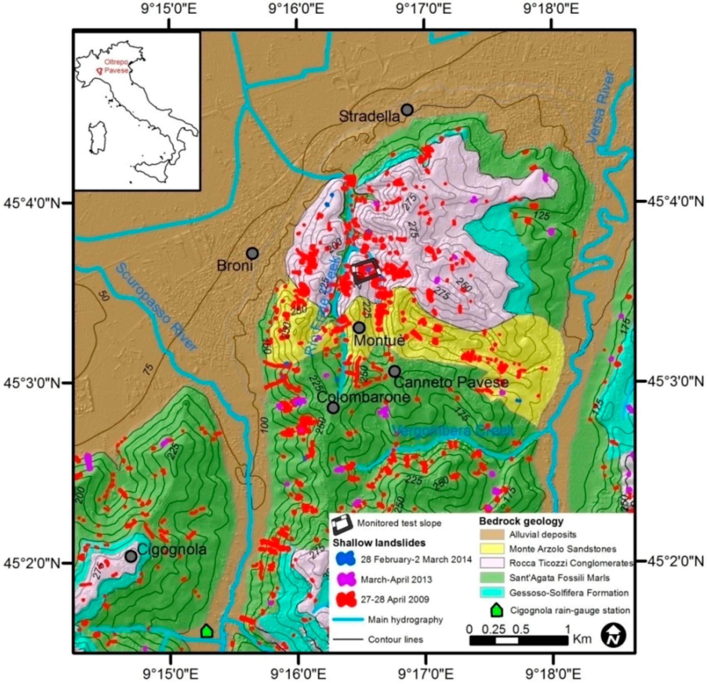
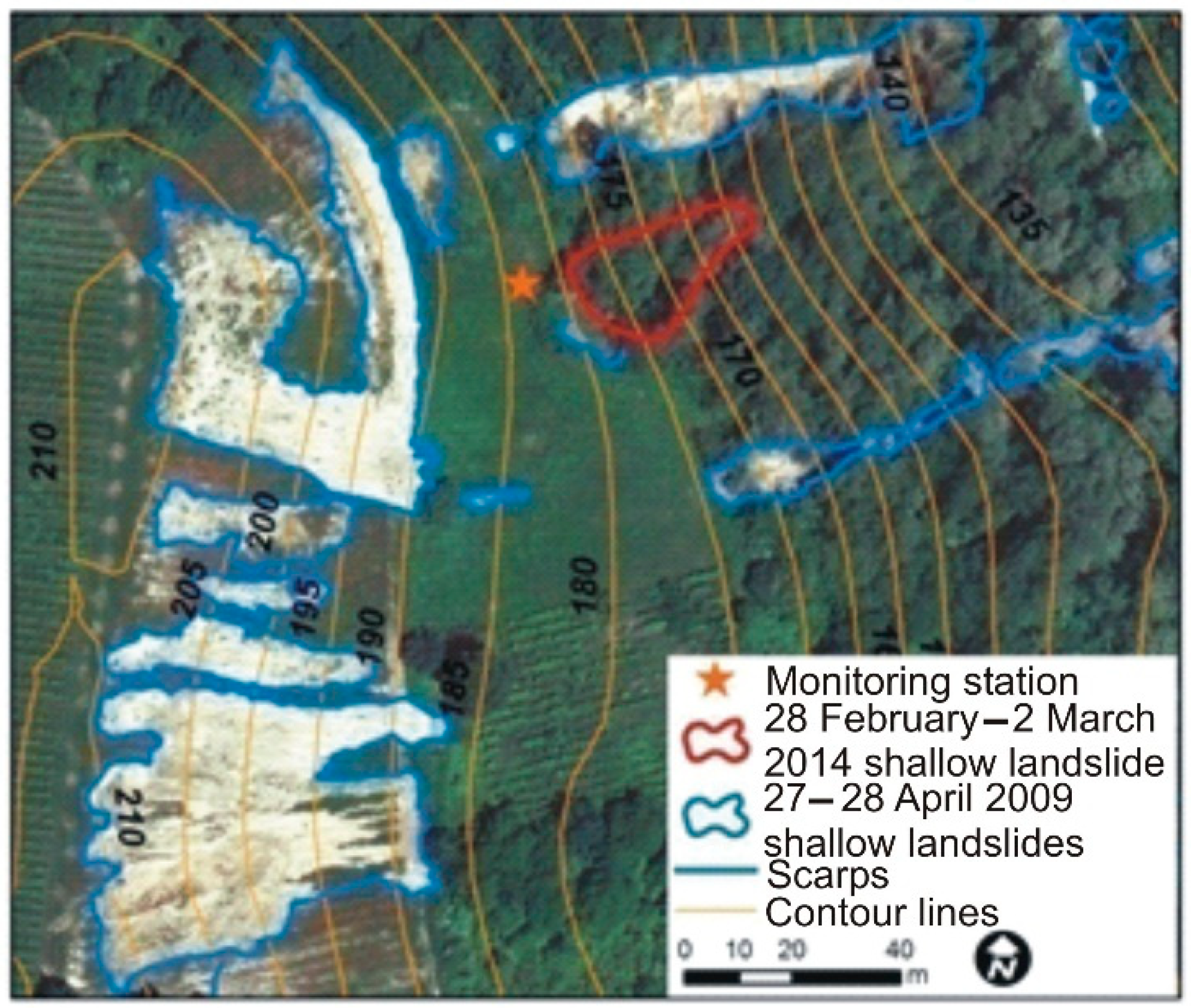
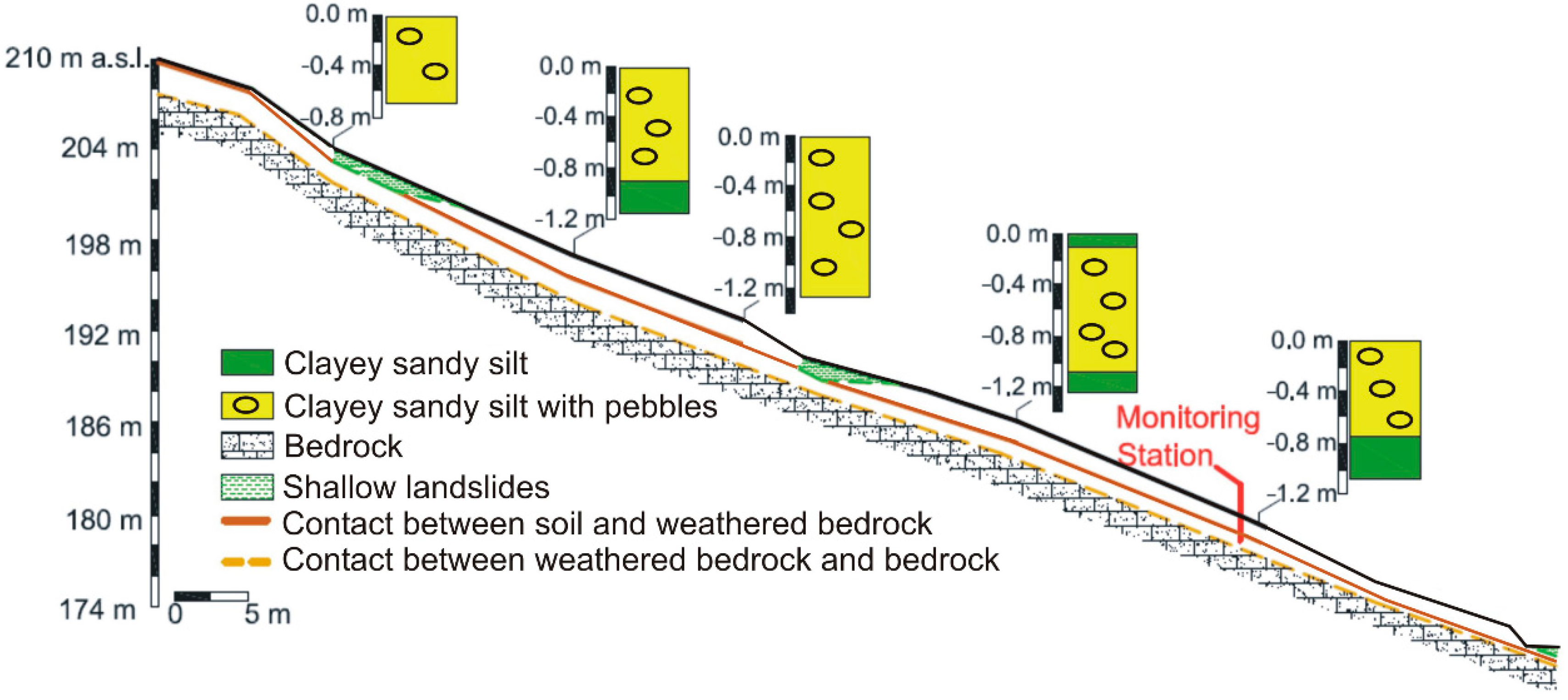
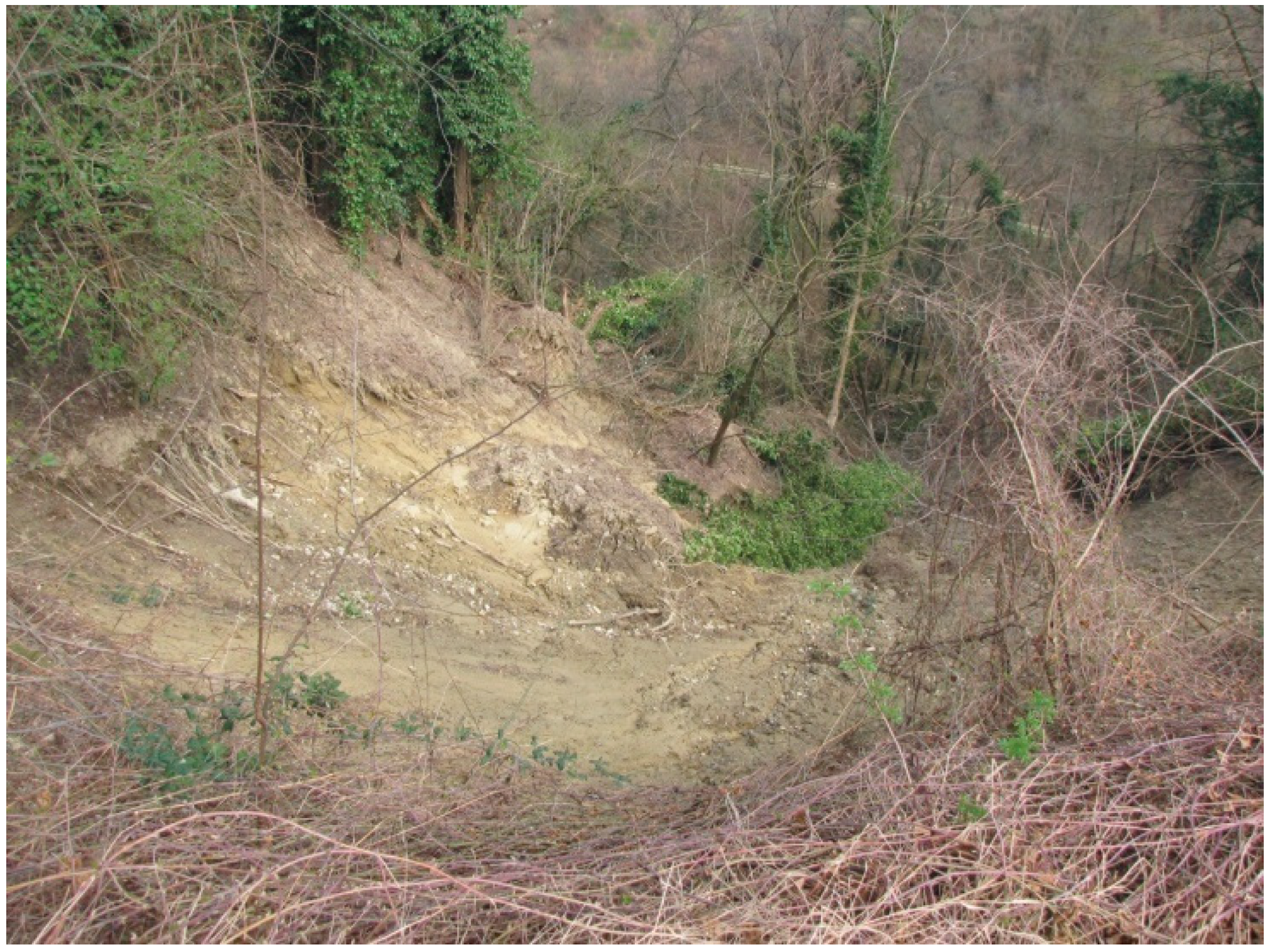
2.1. TestSite Slope Geological Setting and Landslide Distribution

The testsite slope is located in the northeastern part of Oltrepò Pavese (Northern Italy), a hilly region corresponding to the northern termination of the Apennines (Figure 1). In this area, medium-lowpermeability arenaceous–conglomeratic bedrock, including the Monte Arzolo Sandstones and the Rocca Ticozzi Conglomerates, overlies impermeable silty–sandy, marly bedrock (Sant’AgataFossili Marls).The bedrock strata are sub-horizontal and dip east–northeast. The medium-low hydraulic conductivity of the arenaceous–conglomeratic bedrock is linked to its low primary porosity and to the limited number of fractures, which prevent the development of high secondary hydraulic conductivity. Deep-water circulation is thus confined in levels of less cementation or more fracturing at various depths in the bedrock. In the area surrounding the monitored slope, these levels correspond to horizons of poorly cemented gravels, sands, or conglomerates, with limited lateral extension and thickness between 0.2 and 1.0 m. These bodies are more widespread where the bedrock corresponds to the Rocca Ticozzi Conglomerates or the Monte Arzolo Sandstones and are rarer in the Sant’AgataFossili Marls. These bodies do not appear to constitute a continuous, more permeable level that can form a deep aquifer. The presence of water can be identified only in correspondence with the more permeable levels as isolated bodies.
Above the bedrock levels, soils derived by bedrock weathering are present. These soils have dominant silty–clay or sandy–silt textures, and their thicknesses, determined through trench pits and micro boreholes, increase from a few centimeters up to 2.0 m from the top to the bottom of the slopes, owing to the presence of landslide accumulation areas.
During the wet seasons, which include winter and spring, thin perched water tables of 0.1–0.2 m can form in the soils at the contact between the bedrock and the superficial deposits. These formations occur in shallower soil horizons during more intense rainfalls.
This area has a continental climatic regime. In the last 10 years (2005–2014), the mean yearly temperature was 13 °C, and the mean yearly rainfall amount was 719.8 mm, based on measurements acquired at Canevino rain-gauge station by the Regional Agency for Environmental Protection (ARPA Lombardia).
The morphological features of the studied slope can be considered typical of the surrounding area (Figure 2). This slope is characterized by a medium-high topographic gradient with values around 30° in correspondence tothe monitoring station (Figure 3). The slope elevation ranges from 210 to 170 m above sea level (a.s.l.), and the monitoring station is located at 185 m a.s.l. The vegetation types are mainly composed of grass and shrubs, in addition to a woodland of black locust (Robiniapseudoacacia) trees at the bottom of the slope. The roots of the living vegetation are present from the ground surface to depths of about 0.3–0.4 m.
The testsite slope is representative of a wider area characterized by a high density of shallow landslides (Figure 1 and Figure 2). The first and more significant event in terms of the number of triggered landslides occurred on 27–28April 2009. An extreme rainfall of 160 mm in 62 h was measured at the Cigognola rain gauge by the private Cooperative of Oltrepò Pavese Viticulturists—COPROVI (Figure 1) [22]. This extreme rainfall triggered more than 1600 shallow landslides throughout the entire Oltrepò Pavese area [12,22]. The highest density, 51 landslides per km2, was registered in the area surrounding the testsite slope.
Shallow landslides events also occurred during the following periods: March–April 2013 [23], when closely occurring rainfall events occurred with a high cumulative rainfall of 273.9 mm, as measured by the rain gauge of the monitoring station installed in the testsite slope between 1 March 2013and 30 April 2013; and 28 February 2014–2 March 2014, owing to an intense rainfall event of 68.9 mm in 42 h, as registered by the rain gauge of the monitoring station, following 30 rainy days with a cumulative rainfall of 105.5 mm. Although no phenomena were observed in the study slope resulting from the 2013 rainfall events, a shallow landslide was triggered during the 28 February 2014–2 March 2014 event,15 m from the monitoring station (Figure 3 and Figure 4). This location wasin very close proximity to a small scarp that formed during the April 2009 event.
Onthe testsite slope, shallow landslides mainly affected the superficial deposit above the bedrock and the slip surfaces located at depths ranging from 0.5 to 1m from the ground surface, in correspondence with the contact between the soil and the bedrock or at the interfacesofthe soil layers with differences in their hydrological and physical properties. Shallow landslide source areas were developed on slopes slightly steeper than that at the monitoring station, ranging between 30° and 35°. In particular, the source area of the shallow landslide occurring on 2 March 2014 had the same slope angle as that of the monitoring station (30°), and the slip surface was1.0 m belowthe ground level [24].

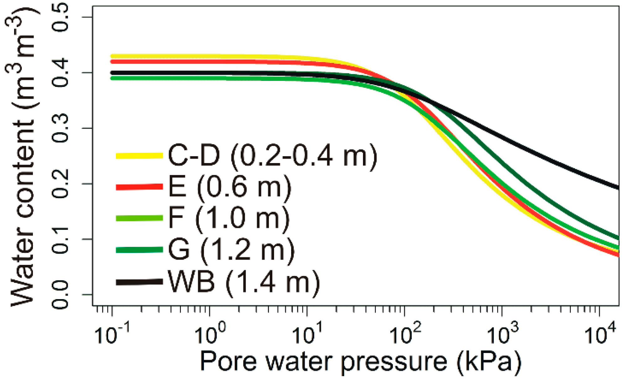
2.2. Soil Characterization at the TestSite Slope

From apedological point of view, the soil profile in the test site is composed of seven main soil horizons (Table 1). The pedological features of the soils were described according to [25]. An organic layer (OL) of 0–0.01 m, dominated by organic soil materials, labeled as A, is the shallowest level. Below this horizon, two weak aggregated levels are present until0.2 m below theground level. A mineral A1 horizon (labeled as B) from 0.01 to 0.1 m exhibits the obliteration of all or much of any original rock structure and shows an accumulation of humified organic matter closely mixed with the mineral fraction. An Ak2 horizon from 0.1to 0.2 m, labeled as C, can be distinguished from the B layer for a high diffusion of carbonate coatings. The soil horizon below the C layer is characterized by a low, strong aggregation. An Apgk3 horizon, from 0.2 to 0.4 m, labeled as D, presents similar structural and pedological features with respect to the overlying layers, but it has a stronger aggregation, an accumulation of visible pedogenic calcium carbonate, and periods of stagnant water, whichhas preserved iron in a reduced state. Moreover, 0.4 m below theground level, the soil horizons are characterized by a lower amount oforganic matter, which shows better the mineral components of the grains of the horizons with respect to the ones close to the surface. A Bgk horizon (labeled as E), located from 0.4to 0.7 m, is a mineral horizon with strong gleying features, which is accompanied by evidence of pedogenic change, while a BCgk horizon (labeled as F) from 0.7to 1.1 m is a transitional horizon that records a subtle lithologic discontinuity, and it is dominated by the properties of the B master horizon. Between 1.1and 1.3 m, a Cgk horizon, labeled as G, is a mineral horizon or a series of layers that arenotaffected greatly by pedogenic processes, and its material is similar tothat from which the solum formed, in that it is characterized by calcic features with an accumulation of carbonates and a significant increase in the carbonate content, reaching35.3%. Weathered bedrock (WB) was identified at a depth of 1.3 m. According to [25], the soil should beclassified as Calcic Gleysol, owing to the presence of a deep calcic horizon (G horizon), where the carbonate content increases to 35.3%. Level G can then be considered to bethe least permeable level of the entire soil profile, as previously shown in similar pedological profiles having a calcic horizon that is at least 0.2-m thick [26]. Regarding the geotechnical and physical properties of the soil, horizons A, B, and C are assumed to havethe same characteristics (Table 1).
The soil horizons have a high silt content of 51.1–65.6%, which tends to increase slightly with depth, andthe clay content is higher than 21.3% (Table 1). The contents of sand and gravel remain low in the soil levels, at 0.5% and 7.5% in the G horizon, respectively. In contrast, the weathered bedrock immediately below the topsoil, with a sand content of 75%, is considered to be a sand lens (Table 1). According to the Unified Soil Classification System (USCS), the soil horizons are prevalently non-plastic or slightly plastic soils (CL), with a liquid limit (wL) of 38.5–41.8% and a plasticity index (PI) of 14.3–17.2%.
The unit weight (γ) shows a significant increase in the F horizon from 16.7 kN/m3 to 18.6 kN/m3 and then remains rather steady with respect to the depth (Table 1). For the E, F, and G horizons, the peak shear strength parameters were determined through triaxial tests (Table 1). The E and F horizons have a friction angle (φʹ) between 31° and 33° and nil cohesion (cʹ). The G horizon is characterized by a friction angle equal to 26° and an effective cohesion of 29 kPa.
The hydrological properties of the various horizons were determined through laboratory reconstruction of SWRCs and HCFs (Figure 5). These functions were reconstructed by using a combination of the Wind–Schindler method (WSM; [28]), including the Hyprop instrument (UMS GmbH; Munich, Germany), and the vapor pressure method (VPM; [29]), including the WP4T device (Decagon Devices; Pullman, DC, USA) on the undisturbed soil samples. The experimental data were fitted through the models of [27,30]. The parameters of these models, including the saturated water content θs, the residual water content θr, the fitting parameters α and µ, and the saturated hydraulic conductivity Ks were then estimated by using the Marquardt algorithm [31]. Although the drying–wetting hysteresis phenomenon of these soils has been deeply investigated elsewhere [24,32], for the purposes of the present work, it has been neglected and the mean values of the Van Genuchten and Mualem parameters have been assumed. All of the soil levels had similar mean values of α (0.007–0.013 kPa−1) and θr (0.01–0.03 m3m−3; Table 2). The µ and θs parameters were slightly higher until the depth of 0.6 m. Moreover, Ks was quite steady around 1 ×·10−6 and 2.5 ×·10−6 ms−1, except for that at the soil level at 1.2 m below the ground (G level), which was the lowest permeable soil horizon (5·× 10−7 ms−1; Table 2). The weathered bedrock (WB)level at 1.4 m below the ground had lower values of both Ks (3·× 10−7ms−1; Table 2) and µ (1.15; Table 2) with respect to the soil layers above, although it wascharacterized by similar values of θs and θr and a higher value of α (0.050 kPa−1) than those in the soil horizons (Table 2).

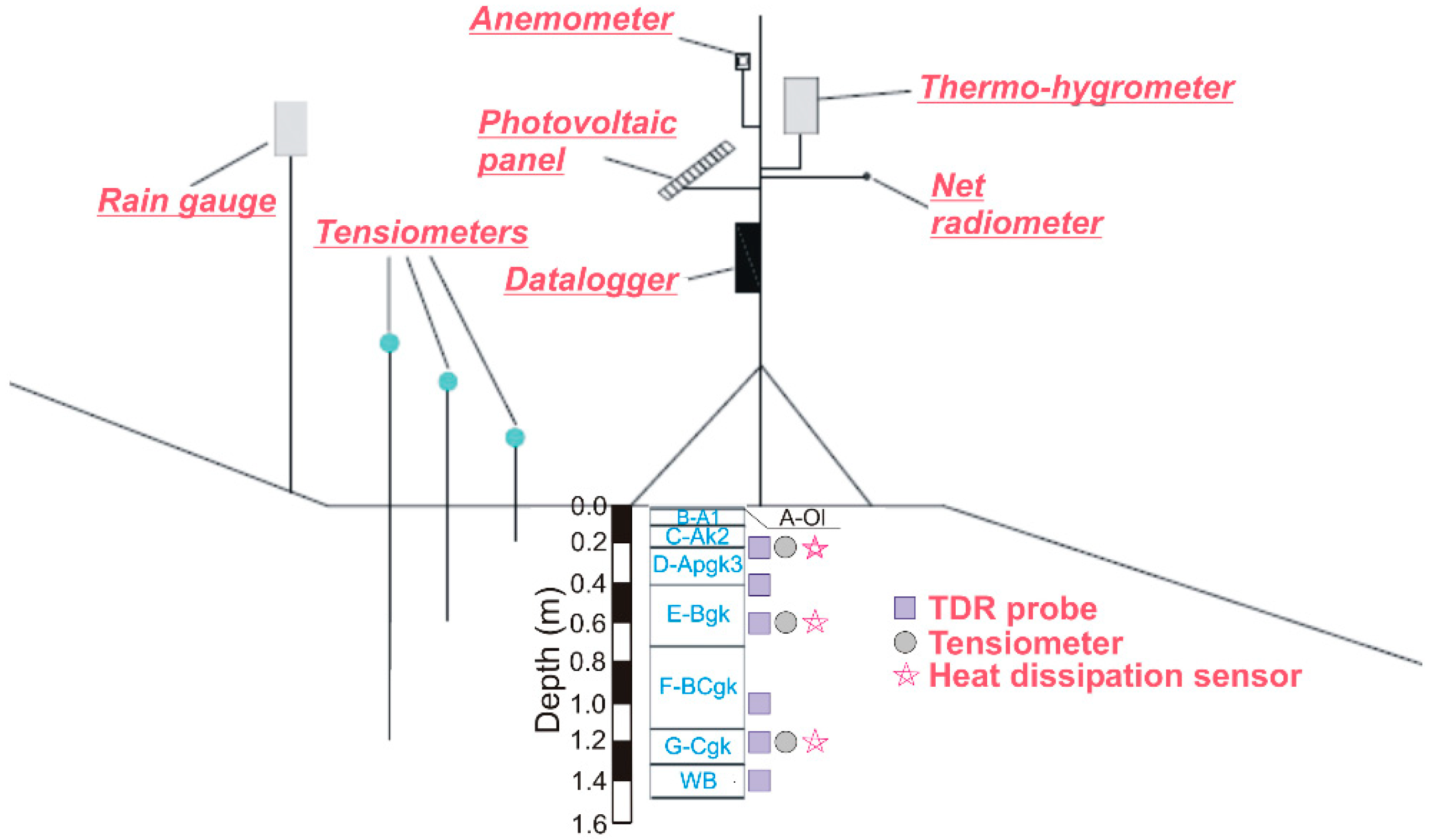
2.3. Monitoring Equipment

The integrated field monitoring station, installed atthe testsite slope on 27 March 2012, consists of a rain gauge (Model 52203, Young Comp., Traverse City, MI, USA), a thermo-hygrometer (Model HMP155A, Campbell Sci. Inc., Logan, UT), a barometer (Model CS100, Campbell Sci. Inc., Logan UT, USA), an anemometer (Model WINDSONIC, Campbell Sci. Inc., Logan, UT, USA), and a net radiometer (Model NR-LITE 2, Kipp&Zonen, Delft, the Netherlands; Figure 6). The meteorological sensors were linked to six time domain reflectometer (TDR) probes (Model CS610, Campbell Sci. Inc., Logan, UT, USA), installed at 0.2, 0.4, 0.6, 1.0, 1.2, and 1.4 m belowthe ground surface, to measure the water content of the soil at various soil levels and that in the weathered bedrock (Figure 6). Moreover, a combination of three tensiometers (Model Jet-Fill 2725, Soilmosture Equipment Corp., Santa Barbara, CA, USA) and three heat dissipation (HD) sensors (Model HD229, Campbell Sci., Logan, UT, USA) were installed at 0.2, 0.6, and 1.2 m belowthe ground level in various soil horizons to measure the pore water pressure [24].
The field data were collected by a CR1000X datalogger (Campbell Sci. Inc., Logan, UT, USA) powered by a photovoltaic panel. A detailed analysis of the quality of the field data has been reported by [24].

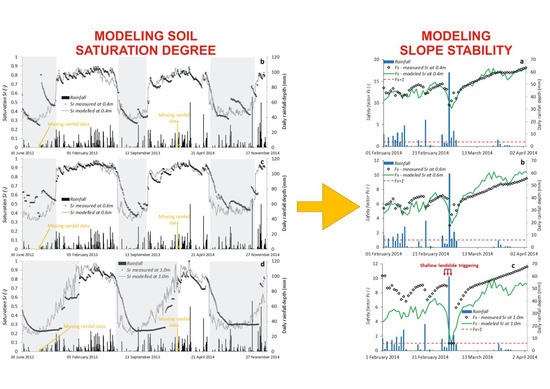
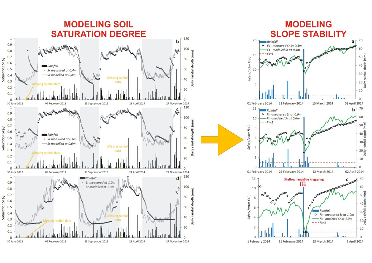
2.4. Modeling the Degree of the Soil Saturation

To perform the slope stability analysis, the degree of thesoil saturation (Sr) at various depths in the soil profile is required (Equation (2)). Table 3 summarizes the input parameters used for the determination of Sr from the field measurements of the water content (θ). Daily average values of Sr were calculated through Equation (2) down to 1m (i.e., the depth of the sliding surface of the shallow landslide observed on 28 February 2014–2 March2014). The main objective was modeling the dynamics of the degree of the soil saturation within the depth at which shallow landslides usually develop in the sample slope. Thus, Sr trends were obtained 0.2, 0.4, 0.6, and 1.0 m belowthe ground surface, based on TDR measurements obtained at the same depths by using the following equation:
S r = S e = θ θ r θ s θ r .
In Equation (2), the degree of saturation is assumed to be equal to the effective saturation, becausethe residual water content is negligible (Table 2). Although the sensitivity analyses of the possible deviations of both the θs and θr values and of the subsequent effects on the chain of models is desirable, such tasks are beyond the scope of this paper.
Moreover, Equation (2) implies the assumption that the soil does not significantly change volume as the degree of the soil saturation decreases (and soil suction increases). This assumption has been considered reasonable for the sample slope soils, which have low compressibility and are free of expansive clays.
The measured values of Sr were compared with the values calculated for the same depths by using the empirical model proposed by [21] (Equation (4)). A detailed derivation of the model is presented elsewhere [21]; only the main statements required for completeness are provided here.
This simplified model considers that shallow soil undergoes drying and wetting phases that are determined by complex climate processes; thus, it allows for the computation of the degree of the soil saturation by using readily available climate data, such as air temperature and daily rainfall. Although these two contributions are not independent of each other, they are considered separately in the model. In particular, the dependence of Sr from the temperature is expressed through an exponential law, in which the exponent is represented by the time-varying air temperature Tm. Such a law allows for the reproduction of the seasonal trend of the degree of thesoil saturation following the mean temperature fluctuations. In fact, air temperature has an indirect effect on the soil moisture, because it is a key variable in the evapo-transpiration process. Therefore, air temperature can be considered to bea good proxy for the seasonal climate processes that affect the soil moisture.
Regarding the dependence of Sr from rainfall, it is well known that the balance between runoff and infiltration is quite complex for unsaturated soils, and many authors have described in detail this phenomenon related to shallow landslides [33,34,35].
In the simplified approach proposed herein, it is considered that the total rainfall amount does not completely infiltrate the soil due to the runoff. For this reason, the portion of the infiltrated rainfall hi* has been defined as follows:
h i * = { h h < ( 1 S r ) n H ( 1 S r ) n H h ( 1 S r ) n H
where h is the daily rainfall depth, n is the soil porosity, and H is the soil layer thickness. Moreover, the model assumes that only a portion of the infiltrated rainfall contributes toraising the degree of thesoil saturation, which is expressed through a constant calibration coefficient β* that includes both runoff and leakage. The reduction of the influence of the rainfall on the soil moisture after a certain lapse of time is expressed by a decreasing exponential relation. At each time step, the degree of the soil saturation is computed through the following equation:
S r = S r ( i n ) e ψ T m + β * n H i = 1 ϖ h i * e ξ ( t t i ) .
Sr is then expressed through the sum of the two main contributions, which could be considered independent from each other. The first one is a function of the time-changing air temperature Tm (in °C); the second one, which considers infiltration, is a function of the daily rainfall depth hi, changing in time as well. For computation, Tm is calculated as a mean of the average daily air temperature in a previous time period of 30 days, after a phase of calibration, which considered the drying speeds on aseasonal scale in the tested slope [21]. The coefficient ψ (in °C−1) assumes the meaning of a numerical damping, and Sr(in) is a calibration parameter linked to the initial state of the soil in terms of saturation. β* expresses the contribution to the degree of saturation given by the amount of infiltrated rainfall, also considering the amount of water thatcould be lost asrunoff and leakage, according to the soil type. The numerical coefficient ξ assumes the meaning of a damping coefficient whose dimension is the inverse of time (i.e., day−1), and t is the day of computation. This coefficient is related to the decrease in the water discharge with an increase in the distance from the soil surface due to differences in soil permeability.
It is expected that ψ should be correlated with the type of soil and its thermal conductivity properties, because the soil moisture response to temperature fluctuation is more rapid for sand than for clay. Moreover, it is expected that ψ is a function of the climate and should express a decrease in the effect given by the air temperature with an increase in the soil depth.
Furthermore, it is expected that parameter ξ should be different for each type of soil in relation to the soil permeability, because greater hydraulic conductivity relates to a more rapid decrease of the accumulated water. As reported in Table 3, a constant value of parameter ξ is selected for the various layers, because they are characterized by the same type of soil.
Indeed, the modeled daily value of Sr represents the average value of the degree of saturation over a soil column of height H, characterized by a given porosity n. In order to apply this model to the described sample site, the degree of saturation was computed at different depths by assuming in each case that the soil column depth (H) was equal to the depth of the measuring point. In other words, to compute Sr of the C soil horizon, H was assumed to be equal to 0.2 m; to compute Sr of the D soil horizon, H was assumed to be equal to 0.4 m; and H was equal to 0.6 m and 1m for soil horizons E and F, respectively. The model calibration was carried out separately for each soil horizon.
Table 3 summarizes the values of the parameters assumed for the model’s application. Parameters ψ, ξ, β*, and Sr(in) were calibrated through an adjustment procedure to get the best fit according to the measured values of Sr over the analyzed time span.
The field measurements clearly showed that compared with the deeper soil horizons, different hydrological and thermal behaviors characterized the soil horizons at shallow depths, where grass and plant roots are usually present [3,20,24]. These differences wereparticularly evident during the dry periods, with a low number of rainfall events, and the wet periods, with events that weremore frequent in time. To consider the different soil behaviors, we assumed different values of parameter ψ for the dry periods and wet periods, indicated in Table 3 as the “wet season” and the “dry season”, respectively, in agreement with the results reported by [36] for similar sites in the Mediterranean area. Table 4 shows the time intervals that have been arbitrarily assumed to bedry seasons. It is worth noting that for the C, D, and E layers a dry period correlating strongly to the “real summer time span” was assumed. On the contrary, for the F layer, even if the starting day of the dry season wasthe same, it was necessary to extend the assumed value of the ψ parameter to a wider lapse of timedue to the delay of the response of deep soil levels to either the drying or wetting periods.
The selected values of the model parameters werein good agreement with those used by [21] for similar types of soil at other sample sites. The input daily value of the air temperature was calculated as a mean of the daily temperatures over the previous 30 days to consider the delay of the soil response to the temperature fluctuations.

2.5. Modeling the Slope Stability

Given the characteristics of the sample slope (Figure 3) and the relatively low thickness of the landslide with respect to its extent, the hypothesis of the infinite slope was appropriate for the stability analysis. Both field-measured and modeled Sr trends were used as the input data in the slope stability model proposed by [5]. A detailed derivation of the model was presented by [5], and a previous application to the test site based only on field measurements was reported by [24].
According to this model, which is based on the limit equilibrium method, the slope safety factor Fs is calculated as follows:
F s = c + ( γ z cos 2 δ σ s ) tan ϕ γ z sin δ cos δ
where c′ is the effective cohesion, γ is the unit weight of the soil, z is the depth below the ground surface where a potential sliding surface could develop, σs is the suction stress, δ is the slope angle, and φ′ is the soil shear strength angle. In Equation (5), σs allows for the calculation of Fs also in unsaturated conditions (Sr < 1.0; [5,37]). This parameter can be determined by considering Sr according to Equation (6) [37]:
σ s = S r α ( S r μ / 1 μ 1 ) 1 μ
where α and μ are the fitting parameters of the Van Genuchten equation, determined through the laboratory assessment of the SWRCs of the investigated soil levels (Table 2 and Figure 5). This relationship allows for calculating Fs based on thedegree of the soil saturation.
Table 5 summarizes the input data for the Lu and Godt model. The slope safety factor Fs was calculated considering a slope angle δ equal to 30.2° (Table 5), at depths of 0.4, 0.6, and 1.0 m belowthe ground level, where Sr was measured. Fs was then determined by considering both the measured and modeled Sr values (Table 5) and by considering the geotechnical properties of the soil measured at the investigated depths (Table 1 and Table 5).

3. Results and Discussions

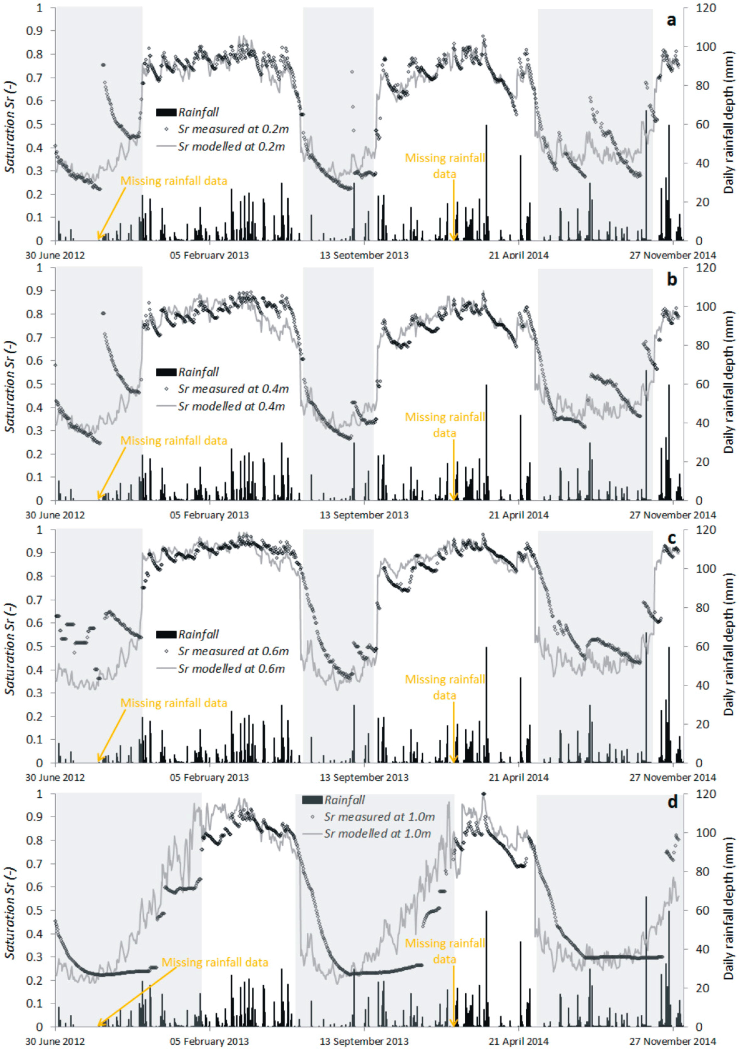
3.1. Comparison between the Measured and Modeled Values of the Degree of the Soil Saturation

Figure 7 shows the time trends of the degree of thesoil saturation calculated through the model of [21] compared with the experimental measurements from the test site, in correlation with the rainfall amount. The Sr values were reconstructed for the time between 30 June 2012 and 5 December 2014, covering about 29 months. The trend analyses began at the start of the first dry period (Table 4). In fact, the first months of the monitoring (between 27 March 2012 and 2 June 2 2012) were disregarded, becauseall the devices needed some time to reach equilibrium and stability.
The modeled and measured values of the degree of saturation were compared at four different depths: 0.2 m (Figure 7a), 0.4 m (Figure 7b), 0.6 m (Figure 7c), and 1.0 m (Figure 7d). The model was not applied to the deepest investigated layers (1.2 and 1.4 m belowthe ground surface) for two main reasons: The first is because previous research has shown that the model is not suitable for reproducing the soil hydrological behavior at depths greater than 1 m [21]. The second is because the observed landslides on the sample slope and in the surrounding zones involved only shallow soils within a thickness of 1m. Figure 7 also shows the indications of two short periods in which rainfall data weremissing: between 31 August 2012 and 4 September 2012 and between 9 and 15 January 2014. For these periods, the model could not attain the values of the degree of saturation at the investigated soil depths due to the lack of rainfall data.
It is interesting to note that in correspondence withall the investigated soil levels, the model reproduced the main hydrological behaviors in response to single rainfall events, particularly during periods of frequent rainfall separated by short time intervals (Figure 7). The horizons up to0.6 m belowthe ground surfaces showthequick response torainfall in terms of increases in the degree of the soil saturation in both dry (summer) and wet (winter) periods (Figure 7a–c). In these shallow layers, the degree of thesoil saturation frequently reaches values up to almost 0.9. For the soil horizon at −1.0 m, only longer rainy periods during the winter provoked an increase of the degree of saturation of up to 0.9 (Figure 7d). The saturated conditions were measured and calculated at −1.0 m only for the event of 18 February 2014–2 March 2014 (Figure 7d), which triggered the shallow landslide near the monitoring station. The instability mechanism on the sample slope appeared to be linked to an increase in the degree of the soil saturation in the deeper soil horizons. This generally occurredas a consequence of an intense rainfall event in the wet season, provoking complete soil saturation (Sr = 1) when the antecedent degree of saturation is higher than 0.8. The permanent completely saturated conditions for 1, 2, and 3 March 2014appear to prove the development of a thin, perched water table starting from the G level at −1.2 m [24]. Prolonged dry periods during summer provoked a significant decrease in the degree of the soil saturation at each investigated layer. The drying phase in the shallow layers down to 0.6 m was faster than that in the deeper soil layers (Figure 7). For each soil layer, the reliability of the calculated values of Sr with respect to the measured values was evaluated by using the rootmeansquare error (RMSE) statistical index (Table 6). The RMSE values were determined by considering three different conditions: all records, a simulation of the dry season, and a simulation of the wet season. It is worth noting that although many assumptions were involved in the evaluation of Sr and all the records, a fair agreement occurred between the model and experimental measurements at −0.2m and −0.4m, as indicated by the RMSE indices equal to 0.07 and 0.08, respectively (Table 6). On the contrary, for the deeper soil layers, the agreement wasweaker, as indicated by an RMSE between 0.11 and 0.14. This wasparticularly true during the dry seasons, when the RMSE indices were0.15–0.16 at 0.6 and 1 m below theground, respectively (Table 6). Generally, for all of the investigated levels, the RMSE values of the wet season weresignificantly lower as compared with the values of the dry season, with differences ranging between 0.05 and 0.10 along the soil profile (Table 6).
The very different performance of the model in different seasons is generally due to thesignificantly different hydrological response of the shallow soil to the climatic variables, such as the air temperature during winter (wet and cold season) and summer (dry and hot season). It should be highlighted that the complex interaction between the soil and the atmosphere cannot be adequately described only by the trend of air temperature and then by a unique set of the model parameters. Two effects in particular weredisregarded by the model: a) the presence of snow, which indeed does not have an immediate influence on the water content of the soil measured during winter; and b) the presence of shrubs and grass during summer, which increases the drying rate because of the water uptake of the plants. For these reasons, particularly during the dry regime, the model wasless efficient. Thus, different sets of parameters were chosen for different seasons.
The arbitrary assumption of varying the input model parameters in correspondence with the selected dates implied that the modeled Sr values underwent a sudden decrease (increase) at the beginning of dry(wet) season with respect to the previous trend. Although this assumption wasnot consistent with the measured degree of saturation, particularly at −0.6 and −1.0 m belowthe ground level (Figure 7c,d), the roughness of the model made it necessary. Two main aspects can be highlighted. The first addresses the poor correspondence between the measured and calculated values of Sr during the first phase of the drying period, particularly for points at depths of −0.6 and −1.0 m.
This is strictly linked with the fact that, at these depths, the soil moisture does not depend only on the air temperature and rainfall. Other more complex processes disregarded by the model, such as the water uptake ofplants, affect the drying of both shallow and deep soil layers.
Second, the drying effect of high air temperatures during summer is progressively delayed at increasing soil depths. With respect to both of these aspects, the model was less accuratein reproducing the actual trend of the degree of the soilsaturation at depths greater than 0.4m below the ground surface in this test site. These results confirm thoseobserved in previous works for other sample sites [21]. On the contrary, during the wet season, when the probability of landslide occurrence is higher, the model has higher accuracy.

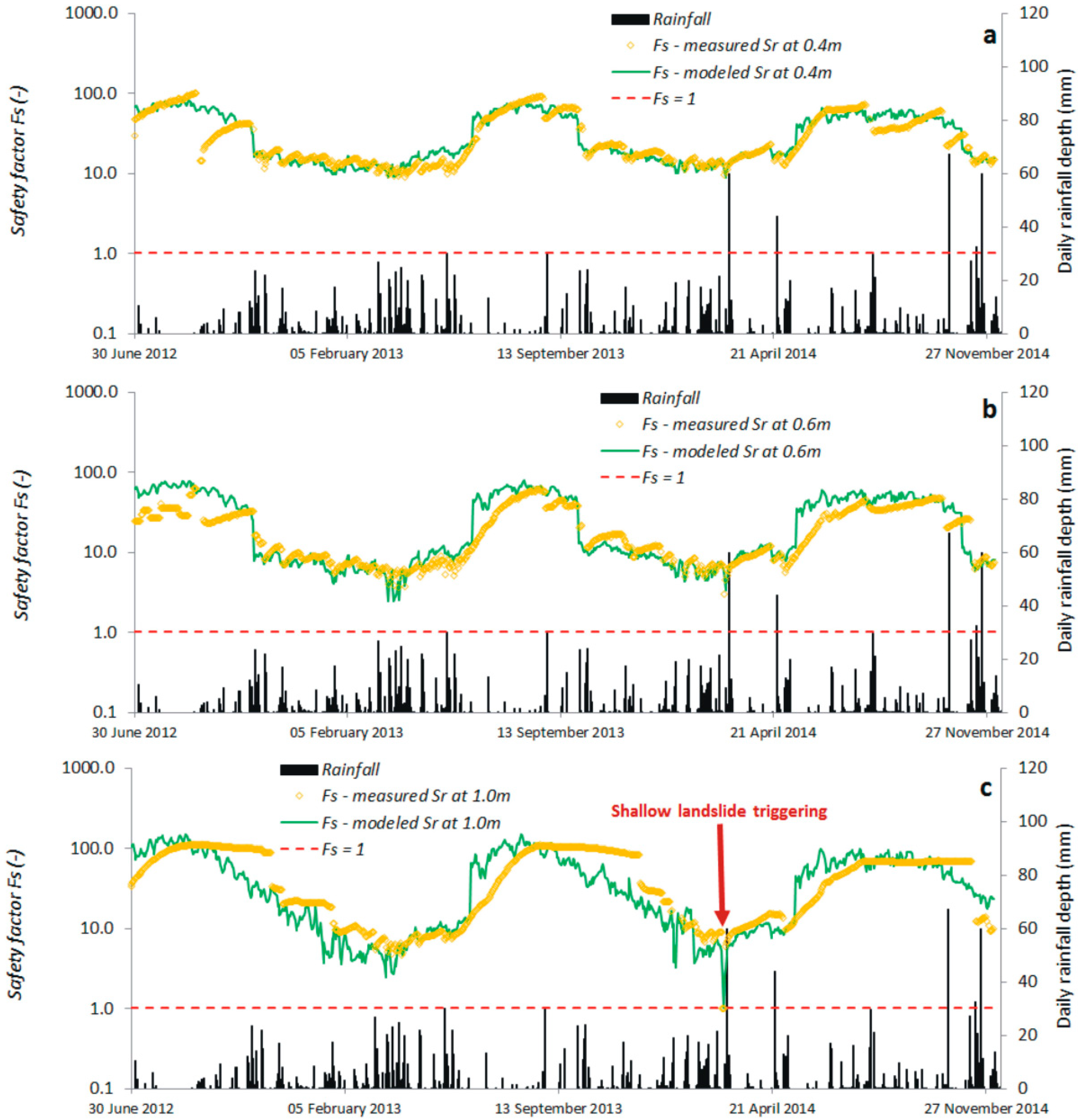
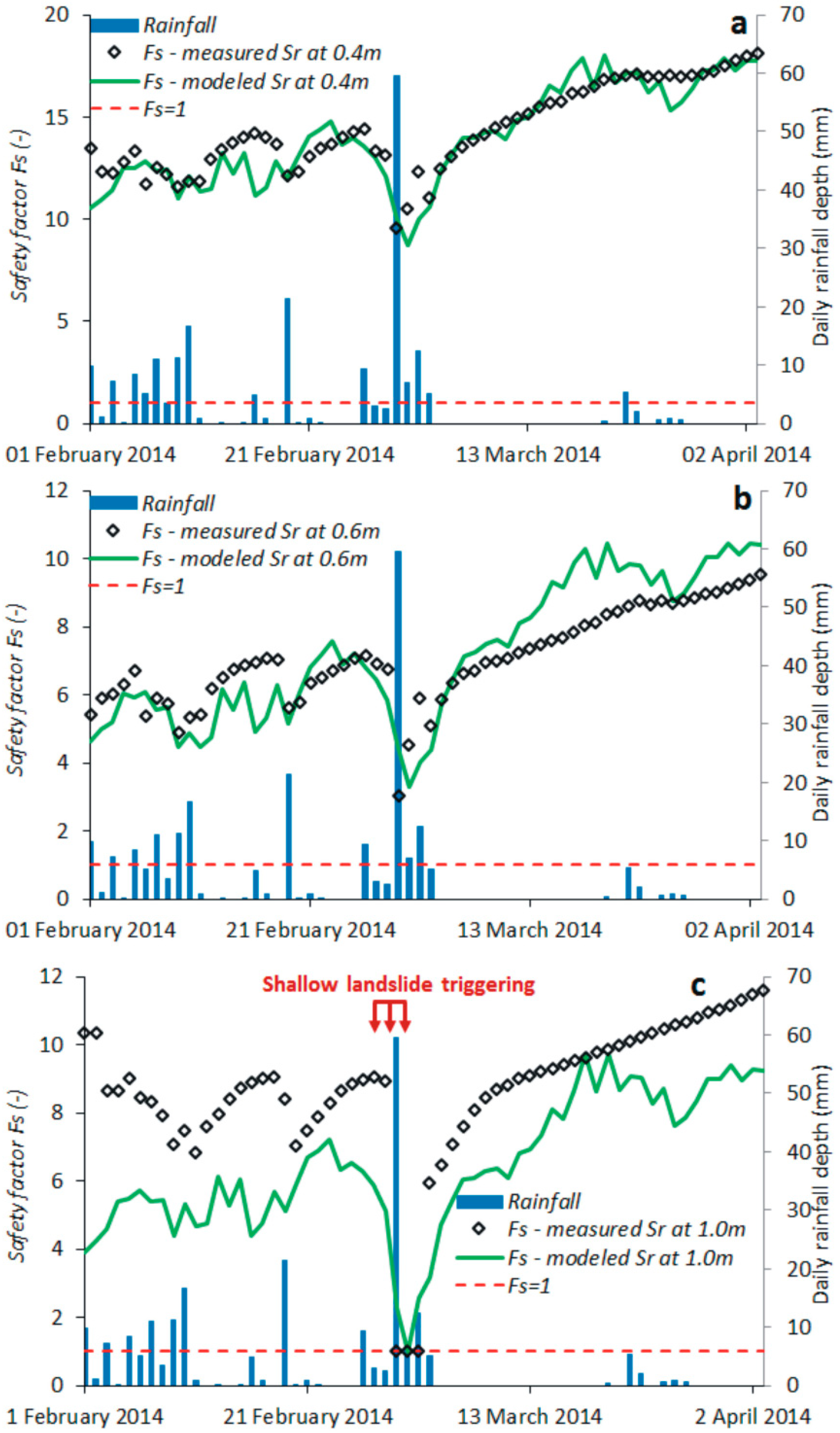
3.2. Slope Safety Factor Trends

The measured and calculated Sr values were used to obtain the Fs trends by using the Lu and Godt slope stability model for the same monitoring time (Figure 8). Fs was calculated for levels at 0.4, 0.6, and 1.0 m below theground level.
In fact, in the testsite slope and in the surrounding slopes with similar geological and geomorphological features, shallow landslides sliding surfaces were located between 0.4 m and 1.0m below the ground level. The reconstruction of the trends at different depths allowed us to investigate the potential differences in the stability conditions at these depths, with the awareness that the sliding surface of the landslide that actually occurred was 1 m below the slope surface.
A rather good agreement between the Fs trends obtained from the measured Sr values and those obtained from the modeled Sr were noted (Figure 8). Similar to that previously observed for the Sr annual cycles, the Fs trends at 0.4m showed a better agreement with respect to the levels at 0.6 m and 1.0 m belowthe ground level (Figure 8). Moreover, the agreement wasmuch more evident in the wet season, when thedegree of the soil saturation was higher than 0.8, and the Fs trends abruptly decreased with respect to the dry season (Figure 8 and Figure 9).
It should be stressed that becauseroots are present at a depth of 0.3–0.4m, root reinforcement can play a role in the slope stability. This root effect has not been included in the analysisin order to obtain a conservative assessment of Fs.
Regarding the shallow landslide occurring between 28 February 2014 and 2 March 2014, both the Fs trends correctly identified the triggering time 1m belowthe ground surface, where the sliding surface actually developed (Figure 8 and Figure 9). In particular, unstable conditions were attained for three days, 1–3March2014, by the Fs trend from the measured Sr but only for one day, 2 March 2014, by the Fs trend from the modeled Sr (Figure 9).

4. Conclusions

Long-term field measurements of the water contents at various soil depths were taken on a sample slope located in the northeastern Oltrepò Pavese (Northern Italy), where several rainfall-induced shallow landslides recently occurred. The measured water contents were used as benchmark values for the calibration and validation of an empirical model able to evaluate the degree of saturation of the soilbased on the air temperature and rainfall data.
The comparison between the measured and modeled vales of the degree of the soil saturation showed that the empirical model was only partially able to reproduce the hydrological conditions at soil depths greater than 0.5 m below the ground surface over the considered period. In particular, the model appeared to be less efficient during dry regimes, although different sets of parameters were chosen for different seasons. Nevertheless, a fair agreement between the modeled degree of thesoil saturation and the experimental measurements were observed at depths of 0.2 m and 0.4 m, particularly during the wet season. Moreover, for the purposes of a simplified approach, the drying–wetting hysteresis phenomenon of the different soil layers was neglected.
Both the measured and modeled values of the degree of saturation were used to obtain the Fs trends of the slope. Fs was calculated by assuming the sliding surface at different soil depths through the slope stability model proposed by [5]. Deliberately, in this research, Fs was calculated on the basis of the soil water content instead of the soil suction, while the two modes were investigated and compared elsewhere [24]. Fairly good correspondence between the Fs trends obtained from both the measured and modeled Sr values was observed. This result appeared useful in the following terms: if Fs, calculated on the basis of measured hydrologic variables, can be considered reliable, on the other hand, in situations where field measurements are lacking, a preliminary evaluation of the slope stability could be carried out based only on the rainfall and air temperature. In particular, the performance of both the Fs trends can be considered rather good in identifying the triggering time and position of the sliding surface of a shallow landslide that actually occurred during the monitoring period in conditions of complete saturation. This result proved that apotential error in the evaluation of the degree of the soil saturation does not substantially affect the assessment of the safety factor. Nonetheless, the assessment of the Fs values appeared to be rather conservative during wet periods (winter), when the occurrence of shallow landslides is more probable, and at higher depths within a soil thickness of 1m, where sliding surface development is prevalent.
It can be concluded that, aside from some limits of the chain of the two models [5,21], the degree of the soil saturation estimated only on the basis of readily available data, such as air temperature and rainfall, can be used as input for the preliminary slope stability analysis. The latter was performed through a simplified limit equilibrium method that appeared to give fairly good results at the slope scale, despite the sharp simplifications introduced for estimating the soil moisture. The proposed approach appears rather promising for application to distributed analysis over large areas, at least for a precautionary assessment of slope stability. However, to provide stability assessment for specific sites, the proposed methodology requires extremely detailed data and appropriate calibration. Moreover, it is worth noting that to apply the same approach to other areas, previous site-specific validation of both models is strongly recommended.
Within the limits of only preliminary analyses on wide areas, the obtained results imply the possibility of assessing the initiation time and depth of shallow landslides oneither a local or regional scale, where only rainfall and air temperature data are available.

Author Contributions

Conceptualization, M.B. and R.V.; Data curation, M.B., R.V., C.M., M.B., and S.C.; Investigation, M.B., M.B., and S.C.; Methodology, M.B., R.V., and C.M.; Supervision, C.M.; Validation, M.B. and M.B.; and Original draft preparation, M.B. and R.V.

Funding

This research received no external funding.

Acknowledgments

We thank Marco Tumiati for hisassistance withthe executions of the laboratory tests on the studied soils. We also thank the anonymous reviewers for their suggestions and contributions to this work.

Conflicts of Interest

The authors declare no conflicts of interest.

References

  1. Corominas, J.; Van Westen, C.; Frattini, P.; Cascini, L.; Malet, J.P.; Fotopoulou, S.; Catani, F.; Van DenEeckhaut, M.; Mavrouli, O.; Agliardi, F.; et al. Recommendations for the quantitative analysis of landslide risk. Bul. Eng. Geol. Environ. 2014, 73, 209–263. [Google Scholar] [CrossRef]
  2. Baum, R.; Savage, W.Z.; Godt, J.W. TRIGRS—A FORTRAN Program for Transient Rainfall Infiltration and Grid-Based Regional Slope-Stability Analysis, Version 2.0, US Geological Survey Open-File 15 Report 2008–1159. Available online: https://pubs.usgs.gov/of/2008/1159/ (accessed on 9 November 2018).
  3. Springman, S.M.; Thielen, A.; Kienzler, P.; Friedel, S. A long-term field study for the investigation of rainfall-induced landslides. Geotechnique 2013, 14, 1177–1193. [Google Scholar] [CrossRef]
  4. Ray, R.L.; Jacobs, J.M. Relationships among remotely sensed soil moisture, precipitation and landslide events. Nat. Hazards 2007, 43, 211–222. [Google Scholar] [CrossRef]
  5. Lu, N.; Godt, J.W. Infinite slope stability under steady unsaturated seepage conditions. Water Resour. Res. 2008, 44, W11404. [Google Scholar] [CrossRef]
  6. Montrasio, L.; Valentino, R. A model for triggering mechanisms of shallow landslides. Nat. Hazards Earth Syst. Sci. 2008, 8, 1149–1159. [Google Scholar] [CrossRef] [Green Version]
  7. Montrasio, L.; Valentino, R.; Corina, A.; Rossi, L.; Rudari, R. A prototype system for space-time assessment of rainfall-induced shallow landslides in Italy. Nat. Hazards 2014, 74, 1263–1290. [Google Scholar] [CrossRef]
  8. Ponziani, F.; Pandolfo, C.; Stelluti, M.; Berni, N.; Brocca, L.; Moramarco, T. Assessment of rainfall thresholds and soil moisture modeling for operational hydrogeological risk prevention in the Umbria region (central Italy). Landslides 2012, 9, 229–237. [Google Scholar] [CrossRef]
  9. Simunek, J.; Van Genucthen, M.T.; Sejna, M. Development and applications of the HYDRUS and STANMOD software packages and related codes. Vadose Zone J. 2008, 7, 587–600. [Google Scholar] [CrossRef]
  10. Granberg, G.; Grip, H.; Löfvenius, M.O.; Sundh, I.; Svensson, B.H.; Nilsson, M. A simple model for simulation of water content, soil frost, and soil temperatures in Boreal mixed mires. Water Resour. Res. 1999, 35, 3771–3782. [Google Scholar] [CrossRef]
  11. Brocca, L.; Melone, F.; Moramarco, T. On the estimation of antecedent wetness conditions in rainfall–runoff modelling. Hydrol. Proc. 2008, 22, 629–642. [Google Scholar] [CrossRef]
  12. Valentino, R.; Meisina, C.; Montrasio, L.; Losi, G.L. Predictive power evaluation of a physically based model for shallow landslides in the area of Oltrepò Pavese, Northern Italy. Geotech. Geol. Eng. 2014, 32, 783–805. [Google Scholar] [CrossRef]
  13. Brocca, L.; Ponziani, F.; Moramarco, T.; Melone, F.; Berni, N.; Wagner, W. Improving landslide forecasting using ASCAT-Derived soil moisture data: A case study of the Torgiovannetto landslide in Central Italy. Remote Sens. 2012, 4, 1232–1244. [Google Scholar] [CrossRef]
  14. Ray, R.L.; Jacobs, J.M.; Ballestero, T.P. Regional landslide susceptibility: spatiotemporal variations under dynamic soil moisture conditions. Nat. Hazards 2011, 59, 1317–1337. [Google Scholar] [CrossRef]
  15. Mittelbach, H.; Seneviratne, S.I. A new perspective on the spatio-temporal variability of soil moisture: temporal dynamics versus time-invariant contributions. Hydrol. Earth Syst. Sci. 2012, 16, 2169–2179. [Google Scholar] [CrossRef] [Green Version]
  16. Godt, J.W.; Baum, R.L.; Lu, N. Landsliding in partially saturated materials. Geophys. Res. Lett. 2009, 36, L02403. [Google Scholar] [CrossRef]
  17. Bittelli, M.; Valentino, R.; Salvatorelli, F.; Pisa, P.R. Monitoringsoil-water and displacement conditions leading to landslide occurrence in partially saturated clays. Geomorphology 2012, 173, 161–173. [Google Scholar] [CrossRef]
  18. Smethurst, J.A.; Clarke, D.; Powrie, D. Factors controlling the seasonal variation in soil water content and pore water pressures within a lightly vegetated clay slope. Geotechnique 2012, 62, 429–446. [Google Scholar] [CrossRef]
  19. Leung, A.K.; Ng, C.W.W. Seasonal movement and groundwater flow mechanism in an unsaturated saprolitic hillslope. Landslides 2013, 10, 455–467. [Google Scholar] [CrossRef]
  20. Bittelli, M.; Tomei, F.; Pistocchi, A.; Flury, M.; Boll, J.; Brooks, E.S.; Antolini, G. Development and testing of a physically based, three-dimensional model of surface and subsurface hydrology. Adv. Water Resour. 2010, 33, 106–122. [Google Scholar] [CrossRef]
  21. Valentino, R.; Montrasio, L.; Losi, G.L.; Bittelli, M. An empirical model for the evaluation of the degree of saturation of shallow soils in relation to rainfalls. Can. Geotech. J. 2011, 48, 795–809. [Google Scholar] [CrossRef]
  22. Zizioli, D.; Meisina, C.; Valentino, R.; Montrasio, L. Comparison between different approaches to modelling shallow landslide susceptibility: a case history in Oltrepò Pavese, Northern Italy. Nat. Hazards Earth Syst. Sci. 2013, 13, 559–573. [Google Scholar] [CrossRef]
  23. Zizioli, D.; Meisina, C.; Bordoni, M.; Zucca, F. Rainfall-triggered shallow landslides mapping through Pleiades images. In Landslide Science for a Safer Geoenvironment; Springer International Publishing: Heidelberg, Germany, 2014; Volume 2, pp. 325–329. [Google Scholar]
  24. Bordoni, M.; Meisina, C.; Valentino, R.; Lu, N.; Bittelli, M.; Chersich, S. Hydrological factors affecting rainfall-induced shallow landslides: from the field monitoring to a simplified slope stability analysis. Eng. Geol. 2015, 193, 19–37. [Google Scholar] [CrossRef]
  25. IUSS Working Group WRB. World Reference for Soil Resources 2006, First Update 2007; World Soil Resources Reports 103; The Food and Agriculture Organization (FAO): Rome, Italy, 2007. [Google Scholar]
  26. Baumhardt, R.L.; Lascano, R.J. Physical and hydraulic properties of a calcic horizon. Soil Sci. 1993, 155, 368–375. [Google Scholar] [CrossRef]
  27. Van Genuchten, M.T. A closed-form equation for predicting the hydraulic conductivity of unsaturated soils. Soil Sci. Soc. Am. J. 1980, 44, 892–898. [Google Scholar] [CrossRef]
  28. Peters, A.; Durner, W. Simplified evaporation method for determining soil hydraulic properties. J. Hydrol. 2008, 356, 147–162. [Google Scholar] [CrossRef]
  29. Rawlins, S.L.; Campbell, G.S. Water potential: Thermocouple Psychrometry. In Methods of Soil Analysis Part 1-Physical and Mineralogical Methods, 2nd ed.; American Society of Agronomy: Madison, WI, USA, 1986; pp. 597–618. [Google Scholar]
  30. Mualem, Y. A new model predicting the hydraulic conductivity of unsaturated porous media. Water Resour. Res. 1976, 12, 513–522. [Google Scholar] [CrossRef]
  31. Marquardt, D.W. An algorithm for least-squares estimation of non-linear parameters. J. Soc. Ind. App. Math. 1963, 11, 431–441. [Google Scholar] [CrossRef]
  32. Bordoni, M.; Bittelli, M.; Valentino, R.; Chersich, S.; Meisina, C. Improving the estimation of complete field soil water characteristic curves through field monitoring data. J. Hydrol. 2017, 552, 283–305. [Google Scholar] [CrossRef]
  33. Cuomo, S.; Della Sala, M. Rainfall-induced infiltration, runoff and failure in steep unsaturated shallow soil deposits. Eng. Geol. 2013, 162, 118–127. [Google Scholar] [CrossRef]
  34. Lanni, C.; McDonnell, J.; Hopp, L.; Rigon, R. Simulated effect of soil depth and bedrock topography on near-surface hydrologic response and slope stability. Earth Surf. Proc. Land. 2013, 38, 146–159. [Google Scholar] [CrossRef]
  35. Shao, W.; Bogaard, T.A.; Bakker, M.; Greco, R. Quantification of the influence of preferential flow on slope stability using a numerical modelling approach. Hydrol. Earth Syst. Sci. 2015, 19, 2197–2212. [Google Scholar] [CrossRef] [Green Version]
  36. Cascini, L.; Sorbino, G.; Cuomo, S.; Ferlisi, S. Seasonal effects of rainfall on the shallow pyroclastic deposits of the Campania region (southern Italy). Landslides 2014, 11, 779–792. [Google Scholar] [CrossRef]
  37. Lu, N.; Godt, J.W.; Wu, D.T. A closed-form equation for effective stress in unsaturated soil. Water Resour. Res. 2010, 46. [Google Scholar] [CrossRef] [Green Version]
Figure 1. Location of the monitored experimental slope and a geological and landslide distribution sketch map of the surrounding area.
Geosciences 08 00472 g001
Figure 2. Detailed view of the testsite slope where the monitoring station was installed, showing evidence of the shallow landslides triggered during the 27–28 April 2009 event. The aerial photograph of the area was captured by Ditta Rossi s.r.l. (Brescia, Italy) on 18 May 2009.
Geosciences 08 00472 g002
Figure 3. Stratigraphic section along the testsite slope [24].
Geosciences 08 00472 g003
Figure 4. Field photograph of the shallow landslide triggered during the 28 February 2014–2 March 2014 event.
Geosciences 08 00472 g004
Figure 5. Soil water retention curves(SWRCs) of the soil horizons at the testsite.
Geosciences 08 00472 g005
Figure 6. Schematic representation of the monitoring station and soil profile.
Geosciences 08 00472 g006
Figure 7. Comparison between the measured and modeled values of the degree of the soil saturation during the monitoring time span at various depths belowthe ground level: (a) 0.2 m; (b) 0.4 m; (c) 0.6 m; and (d) 1.0 m.The grey rectangles represent dry periods.
Geosciences 08 00472 g007
Figure 8. Comparison of the safety factor obtained from the measured and modeled values of the degree of the soil saturation during the monitoring time span at various depths belowthe ground level: (a) 0.4 m; (b) 0.6 m; and (c) 1.0 m.
Geosciences 08 00472 g008
Figure 9. Comparison between the safety factor obtained from the measured and modeled values of the degree of the soil saturation for the period between 1 February 2014 and 3 April 2014 at various depths below the ground level: (a) 0.4 m; (b) 0.6 m; and (c) 1.0 m.
Geosciences 08 00472 g009
Table 1. Main geotechnical, physical, and hydrological properties of the soils at various levels [24].
Soil HorizonRepresentative DepthGravelSandSiltClaywLPIUSCSClassγφ’c’
m%%%%%% kN/m3°kPa
A0.0112.312.553.921.339.817.2CL17.0310.0
B0.1
C0.2
D0.41.611.059.527.938.514.3CL16.7310.0
E0.68.513.251.127.240.315.7CL16.7310.0
F1.02.412.256.429.039.215.9CL18.6330.0
G1.20.57.565.626.441.816.5CL18.22629.0
WB1.40.275.024.80.0--SM18.1
Note: wL: liquid limit; PI: plasticity index; USCS: Unified Soil Classification System; γ: unit weight; φʹ: friction angle; cʹ: cohesion; CL: clay of low plasticity; SM: silty sand; and WB: weathered bedrock.
Table 2. Main hydrological properties of the soil at various levels.
Soil HorizonRepresentative DepthαµθsθrKs
mkPa−1-m3m−3m3m−3ms−1
C0.20.0131.430.430.032.5 × 10−6
D0.40.0131.430.430.032.5 × 10−6
E0.60.0101.400.420.011.5 × 10−6
F1.00.0091.380.390.021.0 × 10−6
G1.20.0071.340.400.015.0 × 10−7
WB1.40.0501.150.400.013.0 × 10−7
Note: α-µ: fitting parameters of Van Genuchten’s [27] model; θs: saturated water content; θr: residual water content; and Ks: saturated hydraulic conductivity.
Table 3. Input data for the calculation of the degree of the soil saturation (Sr).
Soil HorizonDepth mField-Measured SrInput Parameters for Sr Model
θsθrSr(in)β*ξψ (Wet Season)ψ (Dry Season)
m3m−3m3m−3--day−1°C−1°C−1
C0.20.430.030.750.200.080.0150.04
D0.40.430.030.850.200.080.0150.04
E0.60.420.010.920.350.080.0090.04
F1.00.390.020.940.400.080.0150.06
Note: θs: saturated water content; θr: residual water content β*, ξ, and ψ are coefficients.
Table 4. Time spans of dryseasons for the various investigated layers.
Soil HorizonDry Season
FromTo
C, D, E30 June 2012  Geosciences 08 00472 i001
15 June 2013  Geosciences 08 00472 i002
15 May 2014  Geosciences 08 00472 i003
31 October 2012
1 October 2013
31 October 2014
F30 June 2012  Geosciences 08 00472 i004
15 June 2013  Geosciences 08 00472 i005
15 May 2014  Geosciences 08 00472 i006
30 January 2013
30 January 2014
5 December 2014
Table 5. Input data for the Fs model.
Soil HorizonDepth mδSrγφ′c′
°-kN/m3°kPa
C0.230.2Field measured—
Modeled through the model of Valentino et al. [21]
17.031.00.0
D0.4Field measured—
Modeled through the model ofValentino et al. [21]
16.731.00.0
E0.6Field measured—
Modeled through the model ofValentino et al. [21]
16.731.00.0
F1.0Field measured—
Modeled through the model ofValentino et al. [21]
18.633.00.0
Table 6. Rootmeansquare error (RMSE) indices of the modeled trends of the degree of saturation for the investigated soil depths.
Soil HorizonDepth mRMSE
All RecordsDry SeasonWet Season
C0.20.070.100.05
D0.40.080.110.06
E0.60.110.160.06
F1.00.140.150.09

