Abstract
We discuss the influence of different statistical models in the prediction of porosity and litho-fluid facies from logged and inverted acoustic impedance (Ip) values. We compare the inversion and classification results that were obtained under three different statistical a-priori assumptions: an analytical Gaussian distribution, an analytical Gaussian-mixture model, and a non-parametric mixtu re distribution. The first model assumes Gaussian distributed porosity and Ip values, thus neglecting their facies-dependent behaviour related to different lithologic and saturation conditions. Differently, the other two statistical models relate each component of the mixture to a specific litho-fluid facies, so that the facies-dependency of porosity and Ip values is taken into account. Blind well tests are used to validate the final predictions, whereas the analysis of the maximum-a-posteriori (MAP) solutions, the coverage ratio, and the contingency analysis tools are used to quantitatively compare the inversion outcomes. This work points out that the correct choice of the statistical petrophysical model could be crucial in reservoir characterization studies. Indeed, for the investigated zone, it turns out that the simple Gaussian model constitutes an oversimplified assumption, while the two mixture models provide more accurate estimates, although the non-parametric one yields slightly superior predictions with respect to the Gaussian-mixture assumption.
1. Introduction
The Bayesian approach combines the prior knowledge about the model properties with the likelihood function of the data with the aim to estimate the posterior probability distributions of the subsurface properties of interests given the observed data [1,2]. The so computed posterior distribution can be used to estimate the most-likely solution of the inverse problem and to quantify the associated uncertainty. Under some statistical assumptions, the posterior distribution can be analytically derived from the likelihood function and the a-priori information. Otherwise, iterative methods can be employed to numerically assess the posterior model. Analytical methods are often faster than numerical approaches but rely on some limiting assumptions, such as a linear forward operator, Gaussian, Gaussian-mixture or generalized-Gaussian distributions for the model parameters, and a zero-mean Gaussian-distributed error affecting the observed data.
Geophysical inversions are often ill-conditioned, that is multiple solutions can fit the observed data equally well. For this reason, the Bayesian formulation is a convenient way for solving geophysical inverse problems. In particular, the estimation of petrophysical reservoir properties (i.e., porosity, shale content, fluid saturation) and litho-fluid facies around the target area is a common, highly ill-conditioned problem that is often casted into a Bayesian framework [3,4,5,6]. In this context, both analytical and numerical methods have been extensively applied [7,8,9,10,11,12]. The input data to the estimation and classification processes can be logged data (i.e., seismic velocities or seismic impedance values; [13]) or post/pre-stack seismic data [14,15]. In any case, the key ingredient for the estimation of reservoir properties is the petrophysical model that links the elastic attributes (i.e., seismic impedances) to the sought petrophysical properties and/or litho-fluid facies. In this context the main challenge is the fact that petrophysical properties are continuous quantities, whereas the litho-fluid facies are described by discrete variables. To circumvent this issue the estimation process is often solved through a multi-step procedure: first, litho-fluid facies are inferred from the available data (seismic or well log data), then the petrophysical properties are distributed within each facies. Alternatively, over the last years some approaches have been proposed to jointly estimate petrophysical or elastic parameters and litho-fluid facies from the observed data [16,17,18,19].
Independently from the inversion approach adopted (analytical or numerical), the correct choice of the underlying statistical model always plays a crucial role in any geophysical Bayesian inversion. For what concerns the reservoir characterization problem, many authors [20,21,22] have demonstrated that such a statistical model should correctly capture the facies-dependency of petrophysical and/or elastic properties related to the different lithologic and fluid-saturation conditions. According to these authors, accounting for such facies-dependency often provides more accurate descriptions of the uncertainties affecting the sought parameters. However, as the author is aware an in-depth discussion of the results provided by different statistical models is still lacking for reservoir characterization studies. This lack is even more serious as the estimation of reservoir properties and their related uncertainties is of utmost importance for static geological model building, volumetric reserve estimation, and overall field development planning.
In this work, we use an inversion approach for the joint estimation of porosity and litho-fluid facies from logged and post-stack inverted acoustic impedance (Ip) values. The inversion approach that we employ is a modification of the method proposed by [23] that is adapted to consider Gaussian-mixture and Gaussian distributions, and to jointly invert porosity and logged or inverted Ip values. This work is mainly aimed at analyzing and comparing the results that are provided by three different statistical assumptions about the underlying joint distribution of the petrophysical model relating porosity and Ip values: A simple Gaussian assumption, an analytical Gaussian-mixture model, and a non-parametric mixture distribution. The former neglects the facies dependency of porosity and acoustic impedance values, whereas the mixture models relate each component of the mixture to a specific litho-fluid facies. In the context of seismic inversion, the Gaussian or Gaussian-mixture models are often employed because of their many appealing properties; for example, they allow for an analytical computation of the posterior uncertainty and also make the inclusion of additional constraints (i.e., geostatistical constraints) into the inversion kernel possible [18,24]. On the other hand, a non-parametric distribution is not restricted by any statistical assumption about the underlying statistical model, but it impedes an analytical derivation of the posterior model and also complicates the inclusion of additional regularization operators or geostatistical constraints into the inversion framework. These drawbacks often translate into more complex implementations of the optimization algorithm and in an increased computational effort with respect to analytical models. For these reasons, the use of non-parametric distributions in geophysical inversions is more rare than the use of analytical models, although in the last years some inversion strategies based on geostatistical simulations have been proposed [25,26].
This work focuses the attention on well log data pertaining to a gas-saturated reservoir located within a sand-shale sequence. All three considered statistical models are directly estimated from five out of seven available wells drilled through the reservoir zone. In particular, the kernel density technique is used to derive the non-parametric distribution. The two remaining wells are used as blind tests to validate the inversion results, whereas the analysis of the maximum-a-posteriori (MAP) solutions, the coverage ratio, and the contingency analysis tools [27] are employed for a more quantitative assessment of the final predictions. Note, that the lack of reliable logged shear wave velocity information in the target area has impeded the inclusion of additional elastic properties into the petrophysical model. For this reason, we will limit the attention to the estimation of porosity and litho-fluid facies from acoustic impedance values, which is still one routinely used tool in reservoir characterization studies [28,29,30]. We start by introducing the joint inversion approach we use, then the results that were obtained on well log data and seismic inversions are discussed.
2. Methods
In the following we briefly summarized the method proposed by [23] that we use to infer porosity and facies from the impedance values. We refer the reader to [23] for more details. A geophysical forward modelling is usually written as follows:
where is the observed data vector, contains the model parameters, is the noise affecting the data, and is the forward modelling operator. In our case, contains the natural logarithm of logged or inverted acoustic impedance values, whereas the vector expresses the porosity values.
As previously mentioned, the joint estimation of petrophysical properties and litho-fluid facies is complicated by the simultaneous presence of discrete and continuous variables in the model space, that is the distribution of and depends on the underlying facies . In addition, the forward operator could also be facies-dependent (i.e., different rock-physics relations for different facies). After these considerations, the forward modelling of Equation (1) can be rearranged as:
If we consider a Bayesian setting, the goal of the inversion is to estimate the probability of and given the data :
The sought distribution can be numerically computed as [23]:
where, is the joint distribution of porosity and Ip values within each facies, which can be estimated from available well log data. The probability represents the conditional distribution of facies given the observed data that can be computed as:
where is the total number of facies considered: in the following application shale, brine sand, and gas sand.
The key aspect of this inversion approach is the proper choice of the joint distribution . To this end, many assumptions can be made, for example, one can simply neglect the facies dependency of and and thus adopting a simple unimodal Gaussian distribution:
where represents the Gaussian distribution with mean and covariance . Since the facies-dependency is now neglected, this joint distribution can be simply written as . Note that in this Gaussian framework, it is no more possible performing a facies classification. The effectiveness of this statistical model is often case-dependent, and it is related to the underlying petrophysical relation. In the worst case, the Gaussian model constitutes an oversimplified assumption that will lead to biased MAP solutions and non-accurate uncertainty quantifications. However, such an assumption can be suitable for specific exploration targets, as shown in [22]. Generally, the assumed statistical model should honor the multimodality of the distribution, and among the many multimodal distributions, the Gaussian-mixture is often adopted because analytically tractable. In our application, this Gaussian-mixture joint distribution can be written as:
where still represents the Gaussian distribution with facies-dependent mean and covariance values, whereas represents the weight for the n-th component of the mixture with . In other words, the joint distribution of the and is now assumed to be Gaussian within each facies.
Another possible, but less common approach, is to directly approximate the joint distribution using a non-parametric technique, such as the kernel density estimation (KDE). For example, for a univariate random variable , the KDE probability distribution can be computed as:
where is the kernel function, is the total number of data points, and is the kernel width that controls the smoothness of the distribution and it should be set assessed on the available data. In this work, the Epanechnikov kernel is adopted:
In all cases, the distribution can be defined on the basis of available well log data investigating the target area.
The numerical inversion method previously described can be applied to both logged impedance values or to the Ip values inferred from a post-stack seismic inversion. In the following, both of these cases are analyzed: first, we use logged Ip values to infer porosity and facies. Second, we exploit the well log information to compute synthetic seismic traces that, in a first inversion step are converted into Ip values and associated uncertainties that become the input for the following inversion step that is aimed at estimating porosity and litho-fluid facies. In this synthetic application we employ a convolutional forward operator to derive the post-stack seismic trace, whereas a simple analytical least-square Bayesian inversion is adopted to estimate the Ip values and the associated uncertainty from post-stack traces. In case of a one-dimensional (1D) convolutional forward modelling, the seismic stack trace is given by:
where W is the Toeplitz wavelet matrix formed by the samples , and D is the numerical partial differential operator. For simplicity, the post-stack inversion assumes log-Gaussian distributed acoustic impedance values [24]. The inversion aims to minimize the following error function:
where, in our application, refers to the observed post-stack data, contains the predicted Ip values, is the covariance matrix expressing the noise in the data ; ; and, are the covariance matrix and the mean vector of the a-priori Ip distribution and is the seismic convolutional 1D forward operator. Being the forward model linear and being the prior model Gaussian, the posterior Ip distribution is still Gaussian with analytical expressions for the a-posteriori mean vector and covariance matrix ():
In the seismic examples the Chapman-Kolmogorov equation is used to correctly propagate the uncertainty affecting the estimated Ip values into the uncertainties that are associated to the final porosity and facies models:
In all applications, the porosity and facies profiles are derived by applying Equation (4) point-by point to each Ip value derived from well log data or inferred from post-stack seismic inversion. This relies on the assumption that the litho-fluid facies are spatially independent, and that the underlying vertical continuity is preserved due to the continuity of the seismic or well log data. In addition, the adopted formulation assumes that the joint probability distribution of the model parameters and the data is vertically stationary. However, a 1D Markov Chain prior model is employed to vertically constrain the predicted facies profile. For example, on the line of [31], we can write:
in which is a given vertical position, whereas the probability can be obtained from the downward transition matrix estimated from available well log data.
For a quantitative assessment of the facies prediction outcomes, we exploit the contingency analysis tools to compute the reconstruction and the recognition rates. The reconstruction rate represents the percentage of samples belonging to a litho-fluid class (True), which are classified in that class (Predicted). The recognition rate represents the percentage of samples that are classified in a litho-fluid class (Predicted) that actually belongs to that class (True). In both cases, information about under/overestimations can be inferred form the off-diagonal terms, whereas the diagonal terms indicate the percentage of sample correctly classified.
In this work, only the porosity parameter is estimated from Ip values, but the employed method can be also used to estimate other petrophysical properties (i.e., shaliness, fluid saturation) from a set of multiple elastic attributes (i.e., acoustic impedance, shear impedance, and density), as shown in [23]. As a final remark, note that if the forward operator is linear and if the model parameters are Gaussian or Gaussian-mixture distributed, the results provided by the employed numerical inversion (Equations (4) and (5)) coincide with the corresponding Bayesian analytical solutions.
3. Results
3.1. Well Log Data Application
We first describe the two joint mixture-distributions derived from five out of seven available wells that reached the investigated clastic, gas-saturated reservoir (Figure 1). The first is the non-parametric distribution estimated through the kernel density technique; the second is the analytical distribution derived by assuming Gaussian distributed porosity and ln(Ip) values within each facies. As expected, at a first glance we note that the acoustic impedance and the porosity values decrease moving from shale to brine sand and to gas sand. The decrease of the Ip values moving from shale to sand is caused by the different elastic properties of the mineral matrices that are associated to the two litho-facies. Note that the shales are usually stiffer than the sands at the depth interval where the reservoir is located (around 1200–1400 m). Moreover, also note the significant decrease of the Ip value as gas replaces brine in the pore space. This marked fluid-saturation effect on the Ip values is still related to the shallow deep interval at which the reservoir is located. Indeed, it is well known [32] that the depth increase tends to progressively hide the effect of different fluid saturations on the elastic properties, thus making the discrimination between different saturation conditions more problematic. The two distributions (non-parametric and analytical) derived for the shale seem to be very similar, whereas their differences are more prominent for the brine and gas sands. In particular, the Gaussian assumption for the brine sand completely masks the multimodality of the distribution that is instead correctly modelled by the non-parametric model. This multimodality could be related to sands with different mineralogic or textural characteristics. Basing on the estimated distributions, we apply Equations (4) and (5) to infer porosity and litho-fluid facies from the logged acoustic impedance values pertaining to two blind wells that are drilled in the same investigated area (from here on named Well A and B) but not used to derive the distributions of Figure 1.
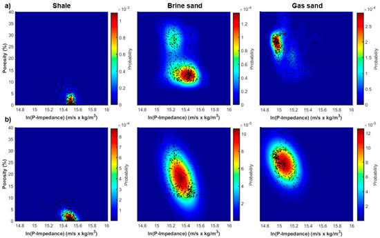
Figure 1.
Non-parametric and Gaussian-mixture joint distributions (parts a, and b, respectively) estimated from five out of seven available wells drilled through the reservoir interval. In (a,b) from left to right we represent the joint distributions pertaining to shale, brine sand, and gas sand. For visualization purposes, the color scales are different for each facies.
Figure 2 represents the results for Well A obtained by considering the non-parametric distribution. In Figure 2a, we observe five significant decreases of the acoustic impedance value that mark the main sand layers embedded in the shale sequence. The target, gas saturated reservoir is located between 1400–1420 m. In Figure 2b, we observe that the MAP solution for the porosity closely matches the actual porosity values and correctly captures the fine-layered structure of the investigated reservoir. The outcomes of the facies classification (Figure 2c–e) show a satisfactory match with the true facies profile derived from borehole information. In particular, Figure 2c clearly depicts the high probability that a gas saturated layer occurs at the target depth (1400–1420 m). Figure 3 shows the results obtained for the same well but employing the Gaussian-mixture distribution. We clearly note (Figure 3b) that the MAP solution for the porosity is now characterized by a poorer match with the logged porosity values than that yielded by the non-parametric model. The facies prediction still shows a satisfactory match with the actual facies profile, and, more importantly, the main gas saturated layer is still correctly identified. For a more quantitative assessment of the recovered posterior porosity distributions, we compute the coverage probability that is the actual probability that the considered interval (in the following the 0.90 probability interval) contains the true property value (Table 1). This statistical measure confirms that the non-parametric distribution yields slightly superior prediction intervals as compared to the Gaussian-mixture assumption. Table 2 displays the linear correlation coefficients between the actual porosity values and the MAP solutions that were provided by the non-parametric and Gaussian-mixture models. The correlation values again prove that the non-parametric model provides final predictions slightly closer to the true porosity model.
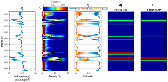
Figure 2.
Inversion results for Well A for a non-parametric . (a) Logged acoustic impedance. (b) Posterior porosity distribution (colour scale), maximum-a-posteriori (MAP) solution (white line), and logged porosity values (black line). (c) Posterior distribution for litho-fluid facies. (d) Actual facies profile derived from well log information. (e) MAP solution for the facies classification. In (d,e) blue, green, and red code shale, brine sand, and gas sand, respectively.
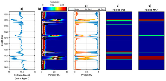
Figure 3.
As in Figure 2, but for the Gaussian-mixture distribution.

Table 1.
Coverage probability values (0.90) for Well A and Well B.
Table 2.
Linear correlation coefficients between the actual porosity profile and the MAP solutions provided by the non-parametric and the Gaussian-mixture models.
Figure 4a,b display the reconstruction and recognition rates associated to Figure 2 and Figure 3, respectively. We observe that the matrices that are represented in Figure 4a,b are similar, although the results for the non-parametric model show larger diagonal terms and lower off-diagonal terms with respect to the results that are provided by the Gaussian-mixture model. This result still demonstrates that that the non-parametric distribution achieves superior classification results than the Gaussian-mixture one.
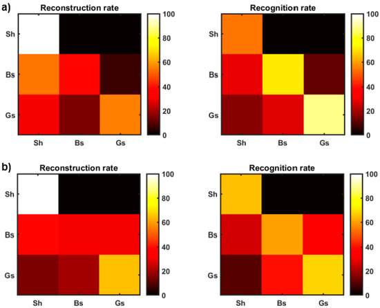
Figure 4.
Reconstruction rate and recognition rate for Well A associated to the non-parametric and Gaussian-mixture distributions (parts a and b, respectively). In (a) and (b) Sh, Bs, and Gs, refer to shale, brine, sand and gas sand, respectively.
Figure 5 shows a direct comparison between the posterior porosity distributions and the actual well log information for two limited depth intervals and for the two tests that are based on the non-parametric and Gaussian-mixture models. For both intervals, we observe that the peaks of the posterior distribution (that is the maximum a-posteriori solutions) yielded by the non-parametric model are closer to the actual porosity values than the MAP solutions that are provided by the Gaussian-mixture assumption. This is a further demonstration that the non-parametric approach estimates a more accurate porosity profile than the analytical one.
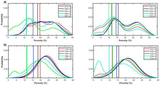
Figure 5.
Direct comparison between posterior porosity distributions (continuous curves) and actual porosity values (vertical lines) extracted for given depth positions. (a,b) refer to the non-parametric and Gaussian-mixture distributions, respectively. In (a,b), the same colour is used for the same depth position.
Figure 6 and Figure 7 display the results yielded by the non-parametric and analytical distributions for Well B, respectively. In this case there is a unique sand layer located between 1170–1183 m in which the fluid saturation passes from predominant gas saturation at the top to a predominant brine saturation at the bottom. The considerations that can be drawn from this experiment are very similar to those derived from the previous tests on Well A, that is the non-parametric distribution yields superior results for both the porosity prediction and, at a lesser extent, for the facies prediction. In particular, the analytical distribution provides a strong underprediction of the porosity values within the depth range 1178–1183 m, whereas the non-parametric distribution correctly identifies a very thin gas-saturated sand layer at 1192 m that is misclassified by the Gaussian-mixture model. The coverage ratios that are associated to this example (Table 1) and the linear correlation coefficients between the actual porosity values and the MAP solutions (Table 2) still confirm that the non-parametric model ensures more reliable predictions, that is a final porosity profile that is closer to the actual values and a posterior solution with superior prediction intervals. In this example, the reconstruction rates and the estimation indexes (Figure 8) pertaining to the two considered distributions are more similar with respects to those resulting from the Well A experiment. The main difference between the two predicted facies profiles is that the non-parametric distribution correctly identifies the gas-saturated layer at 1192 m, while the Gaussian-mixture assumption erroneously predicts a shaly interval at the same depth. This translates into reconstruction and recognition rates for the non-parametric example with slightly higher diagonal terms and slightly lower off-diagonal terms.
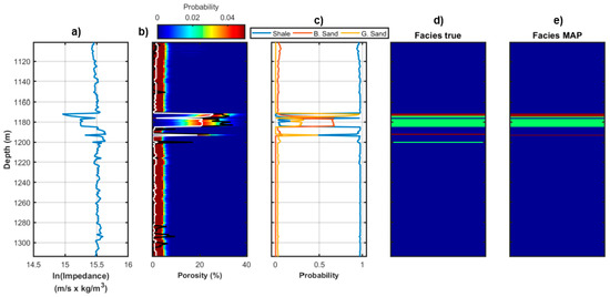
Figure 6.
Inversion results for Well B for a non-parametric . (a) Logged acoustic impedance. (b) Posterior porosity distribution (color scale), MAP solution (white line), and logged porosity values (black line). (c) Posterior distribution for litho-fluid facies. (d) Actual facies profile derived from well log information. (e) MAP solution for the facies classification. In (d,e) blue, green, and red code shale, brine sand and gas sand, respectively.

Figure 7.
As in Figure 6, but for the Gaussian-mixture distribution.
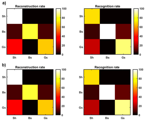
Figure 8.
As in Figure 4, but for Well B.
Similarly to the previous example on Well A, we now represent a direct comparison between the actual porosity values and the estimated posterior porosity distribution along a limited depth interval (Figure 9). Again, this comparison makes clear that the MAP solution that is provided by the non-parametric is characterized by a closer match with the logged porosity values with respect to the corresponding predictions that are achieved by the Gaussian-mixture assumption. In Figure 9b, note that the Gaussian mixture collapses to a simple Gaussian density because the posterior weights of brine and gas sands are negligible with respect to the posterior weight of shale.
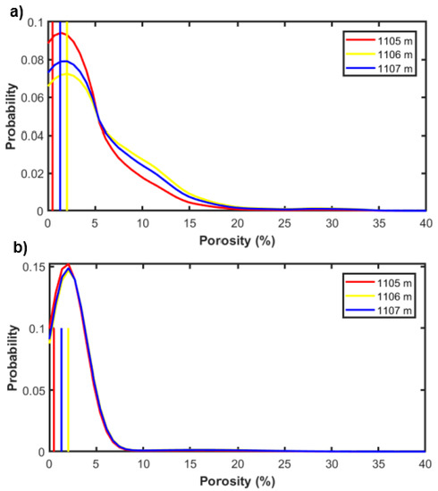
Figure 9.
As in Figure 5, but for Well B.
We now discuss the results obtained when the facies dependency of the porosity and Ip value is neglected, that is when a simple Gaussian distribution is assumed for the joint Ip-porosity distribution. The resulting joint distribution is represented in Figure 10, where we observe that the Gaussian assumption is not able to reliably model the underlying relation linking the porosity and Ip values. In other words, the Gaussian model constitutes an oversimplification of the actual, underlying petrophysical relation. The posterior porosity models that were obtained for Wells A and B are shown in Figure 11a,b, respectively. The MAP solutions still capture the vertical porosity variability but the oversimplified statistical model translates into higher posterior uncertainties (i.e., wider posterior distributions) as compared to the Gaussian-mixture and the non-parametric distributions. In other terms, the suboptimal underlying statistical model results in more inaccurate prediction intervals when compared to the previous tests. The coverage probability values associated to the Gaussian model (Table 3) and the linear correlation coefficients between actual porosity values and MAP solutions (Table 4) quantitatively prove the previous qualitative considerations.
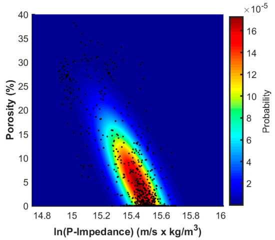
Figure 10.
Gaussian joint distributions estimated from five out of seven available wells drilled through the reservoir interval.
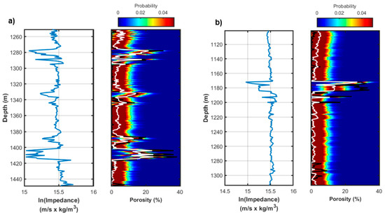
Figure 11.
Inversion results obtained for a simple Gaussian model. (a,b) refer to Well A and Well B, respectively. In both parts the left column represents the actual Ip values, whereas the right column depicts the posterior porosity distribution (color scale), the MAP solution (white line), and the logged porosity values (black line).
Table 3.
Coverage probabilities (0.90) values resulting from the Gaussian assumption.
Table 4.
Linear correlation coefficients between the actual porosity profile and the MAP solutions provided by the Gaussian model.
An example of direct comparison between the true porosity values and the posterior porosity distributions provided by the Gaussian model is represented in Figure 12. For conciseness, we limit the attention to Well A only. Note that in this case the MAP solutions often give suboptimal porosity predictions as compared to the previous examples in which the facies-dependency was taken into account.
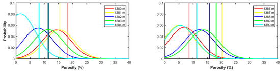
Figure 12.
Direct comparison (for Well A) between posterior porosity distributions (continuous curves) and the actual porosity values (vertical lines) resulting from the Gaussian model. The same colour is used for the same depth location.
3.2. Post-Stack Data Application
We now extend the inversion tests on post-stack seismic data. For confidentiality reasons, we limit the attention to synthetic data computed on the basis of actual well log information and adopting a 1D convolutional forward modelling with a 45-Hz Ricker wavelet as the source signature, and 0.002 s as the sampling interval. To better simulate a field dataset, Gaussian random noise is added to the synthetic stack traces by imposing a signal-to-noise ratio equal to 10. As previously described, in these seismic tests, the inversion is constituted by two cascade steps: first we perform a Bayesian linear post-stack inversion that converts the seismic data into Ip values and associated uncertainties. The outcomes of this first step are the input for the second step of porosity estimation and facies classification. Note that the uncertainties affecting the estimated impedance values are correctly propagated into the estimated porosity and facies profiles through Equation (13). Figure 13 represents the results that were obtained for Well A when the non-parametric distribution is employed. From Figure 13a,b, we note that the predicted seismic trace perfectly matches the observed trace and that the predicted 1D Ip profile (that is represented by the vector; see Equation (12a)) reliably reproduces the vertical variability of the actual impedance values and, more importantly, the 95% confidence interval always encloses the logged Ip. Note that the filtering effect that was introduced by the convolutional forward operator produces Ip predictions with lower vertical resolution with respect to the logged Ip values. Figure 13c compares the MAP porosity solutions with the actual porosity profile. As expected, the filtering effect now translates into less accurate MAP predictions with respect to the well log examples. In particular, the additional uncertainties arising from the seismic inversion yield wider posterior distributions, that is we are now less confident on the final porosity predictions with respect to the previous tests at the well log scale. However, notwithstanding the resolution issue, the inversion still recovers the significant porosity increase that occurs at the sand layers. The estimated facies profile (Figure 13d–f) still shows satisfactory predictions, although the filtering effect provides final result with lower vertical resolution with respect to the previous well log examples.
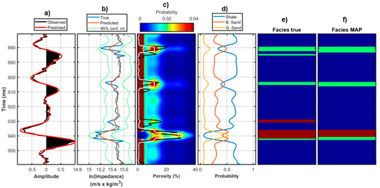
Figure 13.
Inversion results for the synthetic post-stack seismic experiment on Well A for a non-parametric statistical model. (a) Comparison between the observed stack trace (black line) and the predicted trace by the post-stack inversion (red line). (b) Post-stack inversion results. The blue line illustrates the true Ip values (interpolated to the seismic sampling interval), the red line represents the MAP solution (), whereas the green lines delimit the 95% confidence interval. (c) Posterior porosity distribution (colour scale), MAP solution (white line), and logged porosity values interpolated to the seismic sampling interval (black line). (d) Posterior distribution for the litho-fluid facies. (e) Actual facies profile derived from well log information. (f) MAP solution for the facies classification. In (d,e) blue, green, and red code shale, brine sand, and gas sand, respectively.
Figure 14 represents the results for the same Well A but achieved by the Gaussian-mixture model. By the comparison of Figure 13 and Figure 14, we observe that the non-parametric distribution again provides superior porosity estimations and facies profile than the analytical . In particular, only the main gas-saturated layer that is located at 940 ms is correctly identified by the Gaussian-mixture model, while the other sand layers are erroneously misclassified as shaly intervals. The coverage probabilities for the porosity estimation (Table 5), the linear correlation coefficients between actual porosity and MAP solutions (Table 6), and the contingency analysis results (Figure 15) confirm that the non-parametric model outperforms the analytical one.
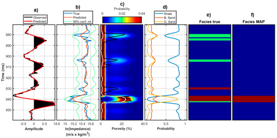
Figure 14.
As in Figure 13, but for the Gaussian-mixture assumption.
Table 5.
Coverage probability values (0.90) for Well A and Well B.
Table 6.
Linear correlation coefficients between the actual porosity profile and the MAP solutions yielded by the non-parametric and the Gaussian-mixture models.
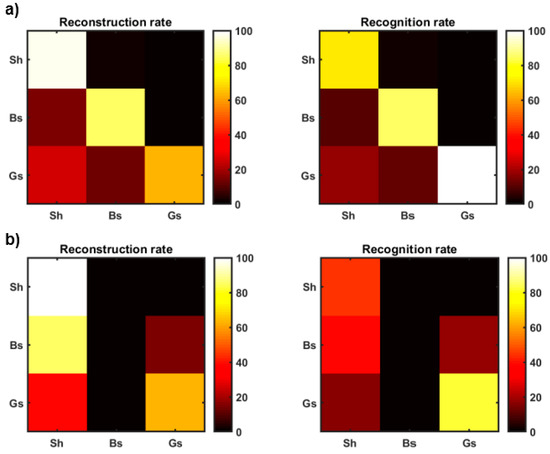
Figure 15.
Contingency analysis results for Well B and pertaining to the non-parametric and Gaussian-mixture distributions (parts a and b, respectively). In (a,b) Sh, Bs, and Gs, refer to shale, brine, sand, and gas sand, respectively.
We now discuss the results for the seismic tests pertaining to Well B (Figure 16 and Figure 17). Again, the non-parametric distribution ensures a more accurate MAP solution for the porosity and superior prediction intervals. Differently from the previous test, the two MAP solutions for the facies profile are now very similar and for this reason the contingency analysis outcomes are not shown here. For this test, the coverage probabilities shown in Table 5, and the linear correlation coefficient between actual porosity model and MAP solutions represented in Table 6, confirm the superior predictions that are given by the non-parametric model.
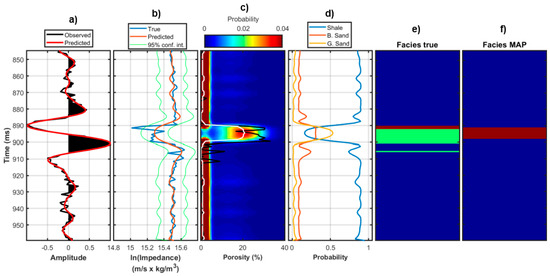
Figure 16.
As in Figure 13, but for Well B.
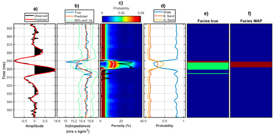
Figure 17.
As in Figure 14, but for Well B.
For the sake of conciseness, the example for the Gaussian model is limited to Well B (similar conclusion would have been drawn from Well A). As expected this statistical model achieves less accurate porosity estimations, higher uncertainties, and less reliable prediction intervals (Figure 18) providing a coverage probability equal to 0.6026 and a MAP solution resulting in a linear correlation coefficient of 0.7718 with the true model; values that are lower than those that are yielded by the Gaussian-mixture and the non-parametric distributions.
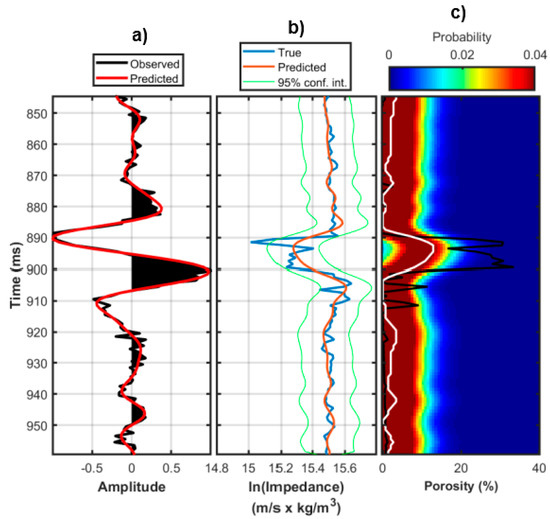
Figure 18.
Inversion results for the synthetic post-stack seismic experiments on Well A when a simple Gaussian model is considered. (a) Comparison between the observed stack trace (black line) and the predicted trace by the post-stack inversion (red line). (b) Post-stack inversion results. The blue line illustrates the true Ip values (interpolated to the seismic sampling interval), the red line represents the MAP solution (), whereas the green lines delimit the 95% confidence interval. (c) Posterior porosity distribution (colour scale), MAP solution (white line), and logged porosity values interpolated to the seismic sampling interval (black line).
4. Discussion and Conclusions
We employed a numerical method for the joint estimation of porosity and litho-fluid facies from logged and post-stack inverted acoustic impedance values. This work was mainly aimed at comparing the porosity and classification results that were obtained under three different statistical assumptions about the joint distribution of porosity and Ip values (): an analytical Gaussian distribution, an analytical Gaussian-mixture model, and a non-parametric mixture distribution estimated via the kernel density algorithm.
The well log and post-stack seismic examples showed that, for the investigated reservoir, the correct modelling of the facies dependency of the porosity and Ip values is crucial to achieve accurate estimations and reliable prediction intervals. Both the Gaussian-mixture and the non-parametric distributions provided satisfactory results (that is results in which the main gas-saturated layers were correctly identified), although the non-parametric statistical model usually achieved superior porosity estimations and litho-fluid facies classifications. Differently, the Gaussian assumption demonstrated to be a too oversimplified model that, totally neglecting the facies-dependency of the porosity and Ip values, provided less accurate prediction intervals, poorer match with actual porosity profiles, and higher uncertainties with respect to both the Gaussian-mixture and the non-parametric statistical models. As expected, in the seismic experiments, the filtering effect that was introduced by the convolutional operator and the additional uncertainties arising from the post-stack seismic inversion, yielded less accurate porosity estimations characterized by wider posterior uncertainties and predicted porosity and facies profiles affected by lower vertical resolution with respect to the examples at the well log scale.
We expect that the introduction of other elastic properties (for example, the shear impedance information) into the petrophysical models, would have better constrained the final porosity and facies predictions, and would also have enabled the joint estimation of other petrophysical parameters, such as shale content, and, in favourable cases, the fluid saturation. However, this fact would have not significantly modified our considerations about the effectiveness of the analysed statistical models.
From the one hand, the conclusions we draw could be not directly extended to all of the geologic settings, as the final results are closely related to the underlying petrophysical model linking the porosity, the Ip values, and the litho-fluid facies. For example, [22,33] for specific exploration areas demonstrated that the Gaussian assumption could be a valid statistical model. On the other hand, an analytical model and a linear forward operator allow for an analytical derivation of the posterior uncertainties. Moreover, an inversion that is based on a simple Gaussian model is not only more easily implementable, but also less computationally demanding than a Gaussian-mixture or a generalized Gaussian assumption. In addition, differently from a non-parametric model, an analytical model allows for the inclusion of additional constraints into the inversion kernel, such as spatial or geostatistical constraints that could be crucial to attenuate the ill-conditioning of the inversion procedure. For example, in a numerical two-dimensional (2D) or three-dimensional (3D) inversion based on a non-parametric distribution and involving continuous and discrete variables, the numerical evaluation of the posterior model at a given location conditioned by the model properties at the adjacent locations rapidly becomes computationally unfeasible as the number of considered neighbouring points increases. For these reasons, the use of non-parametric distributions in 2D or 3D inversions is often challenging.
However, independently from the adopted inversion approach (numerical or analytical), the choice of the statistical petrophysical model is always crucial for the correct estimation of petrophysical properties and litho-fluid facies from well log or seismic data. This choice is often complicated, because it is not only case-dependent, but it must constitute a reasonable compromise between the accuracy of the final predictions, the stability of the inversion procedure, the total computational effort, and the actual fitting between the underlying and the considered petrophysical models.
Funding
This research received no external funding.
Conflicts of Interest
The author declares no conflict of interest.
References
- Duijndam, A.J.W. Bayesian estimation in seismic inversion. Part I: Principles. Geophys. Prospect. 1988, 36, 878–898. [Google Scholar] [CrossRef]
- Tarantola, A. Inverse Problem Theory and Methods for Model Parameter Estimation; Siam: Philadelphia, PA, USA, 2005. [Google Scholar]
- Avseth, P.; Mukerji, T.; Mavko, G. Quantitative Seismic Interpretation; Cambridge University Press: Cambridge, UK, 2005. [Google Scholar]
- Doyen, P.M. Seismic Reservoir Characterization: An Earth Modelling Perspective; EAGE: Houten, The Netherlands, 2007. [Google Scholar]
- Bosch, M.; Mukerji, T.; Gonzalez, E.F. Seismic inversion for reservoir properties combining statistical rock physics and geostatistics: A review. Geophysics 2010, 75, 75A165–75A176. [Google Scholar] [CrossRef]
- Aleardi, M.; Ciabarri, F. Assessment of different approaches to rock-physics modeling: A case study from offshore Nile Delta. Geophysics 2017, 82, MR15–MR25. [Google Scholar] [CrossRef]
- Mavko, G.; Mukerji, T. A rock physics strategy for quantifying uncertainty in common hydrocarbon indicators. Geophysics 1998, 63, 1997–2008. [Google Scholar] [CrossRef]
- Bachrach, R. Joint estimation of porosity and saturation using stochastic rock-physics modeling. Geophysics 2006, 71, O53–O63. [Google Scholar] [CrossRef]
- Gunning, J.; Glinsky, M.E. Detection of reservoir quality using Bayesian seismic inversion. Geophysics 2007, 72, R37–R49. [Google Scholar] [CrossRef]
- Bosch, M.; Cara, L.; Rodrigues, J.; Navarro, A.; Díaz, M. A Monte Carlo approach to the joint estimation of reservoir and elastic parameters from seismic amplitudes. Geophysics 2007, 72, O29–O39. [Google Scholar] [CrossRef]
- Rimstad, K.; Avseth, P.; Omre, H. Hierarchical Bayesian lithology/fluid prediction: A North Sea case study. Geophysics 2012, 77, B69–B85. [Google Scholar] [CrossRef]
- Aleardi, M.; Ciabarri, F.; Mazzotti, A. Probabilistic estimation of reservoir properties by means of wide-angle AVA inversion and a petrophysical reformulation of the Zoeppritz equations. J. Appl. Geophys. 2017, 147, 28–41. [Google Scholar] [CrossRef]
- Grana, D.; Bronston, M. Probabilistic formulation of AVO modeling and AVO-attribute-based facies classification using well logs. Geophysics 2015, 80, D343–D354. [Google Scholar] [CrossRef]
- Mazzotti, A.; Zamboni, E. Petrophysical inversion of AVA data. Geophys. Prospect. 2003, 51, 517–530. [Google Scholar] [CrossRef]
- Eidsvik, J.; Avseth, P.; Omre, H.; Mukerji, T.; Mavko, G. Stochastic reservoir characterization using prestack seismic data. Geophysics 2004, 69, 978–993. [Google Scholar] [CrossRef]
- Kemper, M.; Gunning, J. Rock Physics Driven Joint Inversion to Facies and Reservoir Properties. ASEG Extended Abstr. 2012, 2012, 1–4. [Google Scholar] [CrossRef]
- Gunning, J.S.; Kemper, M.; Pelham, A. Obstacles, challenges and strategies for facies estimation in AVO seismic inversion. In Proceedings of the 76th EAGE Conference and Exhibition, Amsterdam, The Netherlands, 16–19 June 2014. [Google Scholar] [CrossRef]
- De Figueiredo, L.P.; Grana, D.; Santos, M.; Figueiredo, W.; Roisenberg, M.; Neto, G.S. Bayesian seismic inversion based on rock-physics prior modeling for the joint estimation of acoustic impedance, porosity and lithofacies. J. Comput. Phys. 2017, 336, 128–142. [Google Scholar] [CrossRef]
- Gunning, J.; Sams, M. Joint facies and rock properties Bayesian amplitude-versus-offset inversion using Markov random fields. Geophys. Prospect. 2018, 66, 904–919. [Google Scholar] [CrossRef]
- Rimstad, K.; Omre, H. Impact of rock-physics depth trends and Markov random fields on hierarchical Bayesian lithology/fluid prediction. Geophysics 2010, 75, R93–R108. [Google Scholar] [CrossRef]
- Grana, D.; Fjeldstad, T.; Omre, H. Bayesian Gaussian-mixture linear inversion for geophysical inverse problems. Math. Geosci. 2017, 49, 493–515. [Google Scholar] [CrossRef]
- Aleardi, M.; Ciabarri, F.; Gukov, T. A two-step inversion approach for seismic-reservoir characterization and a comparison with a single-loop Markov-Chain Monte Carlo algorithm. Geophysics 2018, 83, R227–R244. [Google Scholar] [CrossRef]
- Grana, D. Joint facies and reservoir properties inversion. Geophysics 2018, 83, M15–M24. [Google Scholar] [CrossRef]
- Buland, A.; Omre, H. Bayesian linearized AVO inversion. Geophysics 2003, 68, 185–198. [Google Scholar] [CrossRef]
- Azevedo, L.; Nunes, R.; Soares, A.; Mundin, E.C.; Neto, G.S. Integration of well data into geostatistical seismic amplitude variation with angle inversion for facies estimation. Geophysics 2015, 80, M113–M128. [Google Scholar] [CrossRef]
- Sabeti, H.; Moradzadeh, A.; Ardejani, F.D.; Azevedo, L.; Soares, A.; Pereira, P.; Nunes, R. Geostatistical seismic inversion for non-stationary patterns using direct sequential simulation and co-simulation. Geophys. Prospect. 2017, 65, 25–48. [Google Scholar] [CrossRef]
- Sammut, C.; Webb, G.I. Encyclopedia of Machine Learning; Springer Science & Business Media: Berlin, Germany, 2011. [Google Scholar]
- Çemen, I.; Fuchs, J.; Coffey, B.; Gertson, R.; Hager, C. Correlating Porosity with Acoustic Impedance in Sandstone Gas Reservoirs: Examples from the Atokan Sandstones of the Arkoma Basin, South Eastern Oklahoma. In Proceedings of the AAPG Annual Convention and Exhibition, Pittsburgh, PA, USA, 19–22 May 2013; p. 41255. [Google Scholar]
- Jafari, M.; Nikrouz, R.; Kadkhodaie, A. Estimation of acoustic-impedance model by using model-based seismic inversion on the Ghar Member of Asmari Formation in an oil field in southwestern Iran. Lead. Edge 2017, 36, 487–492. [Google Scholar] [CrossRef]
- Das, B.; Chatterjee, R.; Singha, D.K.; Kumar, R. Post-stack seismic inversion and attribute analysis in shallow offshore of Krishna-Godavari basin, India. J. Geol. Soc. India 2017, 90, 32–40. [Google Scholar] [CrossRef]
- Larsen, A.L.; Ulvmoen, M.; Omre, H.; Buland, A. Bayesian lithology/fluid prediction and simulation on the basis of a Markov-chain prior model. Geophysics 2006, 71, R69–R78. [Google Scholar] [CrossRef]
- Avseth, P.; Flesche, H.; Van Wijngaarden, A.J. AVO classification of lithology and pore fluids constrained by rock physics depth trends. Lead. Edge 2003, 22, 1004–1011. [Google Scholar] [CrossRef]
- Aleardi, M.; Ciabarri, F.; Calabrò, R. Two- and single-stage seismic-petrophysical inversions applied in Nile Delta. Lead. Edge 2018, 37, 510–518. [Google Scholar] [CrossRef]
© 2018 by the author. Licensee MDPI, Basel, Switzerland. This article is an open access article distributed under the terms and conditions of the Creative Commons Attribution (CC BY) license (http://creativecommons.org/licenses/by/4.0/).