Article

Efficiency of a Digital Particle Image Velocimetry (DPIV) Method for Monitoring the Surface Velocity of Hyper-Concentrated Flows

by
Donatella Termini
* and
Alice Di Leonardo
Department of Civil, Enviromental, Aerospace, Materials Engineering (DICAM), Viale delle Scienze, 90128 Palermo, Italy
*
Author to whom correspondence should be addressed.
Geosciences 2018, 8(10), 383; https://doi.org/10.3390/geosciences8100383
Submission received: 9 August 2018 / Revised: 14 October 2018 / Accepted: 16 October 2018 / Published: 19 October 2018
(This article belongs to the Special Issue Laboratory Geosciences: Modelling Surface Processes)

Abstract

:
Digital particle image velocimetry records high resolution images and allows the identification of the position of points in different time instants. This paper explores the efficiency of the digital image-technique for remote monitoring of surface velocity and discharge measurement in hyper-concentrated flow by the way of laboratory experiment. One of the challenges in the application of the image-technique is the evaluation of the error in estimating surface velocity. The error quantification is complex because it depends on many factors characterizing either the experimental conditions or/and the processing algorithm. In the present work, attention is devoted to the estimation error due either to the acquisition time or to the size of the sub-images (interrogation areas) to be correlated. The analysis is conducted with the aid of data collected in a scale laboratory flume constructed at the Hydraulic laboratory of the Department of Civil, Environmental, Aerospace and of Materials Engineering (DICAM)—University of Palermo (Italy) and the image processing is carried out by the help of the PivLab algorithm in Matlab. The obtained results confirm that the number of frames used in processing procedure strongly affects the values of surface velocity; the estimation error decreases as the number of frames increases. The size of the interrogation area also exerts an important role in the flow velocity estimation. For the examined case, a reduction of the size of the interrogation area of one half compared to its original size has allowed us to obtain low values of the velocity estimation error. Results also demonstrate the ability of the digital image-technique to estimate the discharge at given cross-sections. The values of the discharge estimated by applying the digital image-technique downstream of the inflow sections by using the aforementioned size of the interrogation area compares well with those measured.

1. Introduction

Accurate knowledge of flow discharge is of crucial importance especially for hydrologist and fluvial geomorphologists. In a context of a changing climate, significant hazards associated with both floods and debris or mud flows occur more and more frequently, causing significant changes in topography and river morphology [1].
Traditional techniques usually are based on current-meter measurements (from bridges or set across the channel width) and on the linking of water depth with the discharge through the rating flow velocity curve. Due to the limited accuracy of the current-meter, more modern and accurate instruments, such as Acoustic Doppler Velocimeters (ADV), are also used to measure distribution [2,3]. But, the use of the aforementioned measurement techniques presents many practical difficulties and requires long acquisition times. In particular, Acoustic Doppler Velocimeters require water depths that limit their use in shallow water flows. For this reason, these techniques are essentially limited to low flow conditions inducing high uncertainty in rating curve extrapolation for higher stages. In fact, high flow conditions, characterized by high velocities, large water depths, and high sediment concentrations do not permit the use of the traditional measurement equipment and are not safe for operators because flow depth can significantly change and high flow velocities and floating debris occur [3].
Thus, in recent years, many efforts have been made both to develop techniques capable of providing reliable velocity measurements under challenging conditions and to identify alternative methods to estimate water discharge. As an example, some researchers [4,5,6], based on the application of the entropic concept, suggested to evaluate the mean flow velocity, and de facto the discharge, through the information of the surface velocity, with the great benefit of having quick measurement and high safety for the person involved in measurement. Other researchers have suggested to associate the information of surface velocity with the water level information, leading the estimation either of the depth-averaged velocity value by applying the dimensionless logarithm law [7] or of the water discharge [8].
In such a context, in the last decade, because of improvement of computing capabilities, image-based techniques have been increasingly used for surface velocity measurements in field [7,8,9,10] and in laboratory channels [11,12,13,14].
The advantages of image-based techniques compared to traditional techniques are essentially related to the fact that they are non-intrusive and allow obtaining simultaneous spatial information about the instantaneous velocity components also in unsteady flows [7]. Thus, it is possible to yield a large amount of data in a rather short measuring time and to calculate simultaneously the average values for identical spatial windows over many images. Consequently, quantitative measurement of fluid velocity vectors at a very large number of points could be obtained simultaneously and with a very low cost [15,16,17].
In field applications, large scale PIV (LSPIV) technique has been used to measure the surface flow velocities especially in complex situations such as at junctions between channels or around hydraulic structures [8,9,10,11,12,13,14,15,16,17,18]. In laboratory channels, the conventional PIV technique has been especially used to estimate surface velocity in very small water depths which make the use of direct measurements with traditional equipment impractical [19].
There are some differences between field and laboratory applications of imaging technique [20]. Large scale PIV (LSPIV) covers larger field of view and uses more inexpensive (even natural) illumination devices than conventional PIV [18]. Furthermore, if the flow is dense enough, the objects carried by it could be used as traceable patterns so that artificial seeding is required only when few natural tracers are visible at the surface of the flow. In this case, the tracers need to be larger than the resolution of one pixel to be followed, while in laboratory PIV applications, flow is seeded with microparticles. Thus, recently, image techniques have been also used for hyper-concentrated flows also in laboratory channels [21,22]. The high density of the natural grains allows an easier application of the PIV procedure with natural tracers but, since the granular material is non-transparent, the measurements inside the flow are generally impossible so that the laser sheets are inadequate to illuminate the particles and alternative lighting systems, such as halogen lamps, have to be used [22]. Pudasaini et al. [23,24] employed flashes, Sheng et al. [25] used halogen lamps powered by a flickering-free ballast, Sarno et al. [26,27,28] employed a high-brightness no-flicker LED lamp.
The application of image-based techniques in hyper-concentrated flows is still matter of debate, especially in relation to the opportunity to use moving grains as natural tracers and to the identification of the acquisition time determining adequate number of images to be processed.
From the aforementioned, it is clear that, especially in LSPIV applications, appropriate analyses and processing procedures have to be used in order to obtain quantitative information by applying image-based techniques [22,29]. One of the challenges in the application of image-techniques is the determination of the error in estimating surface velocity. The error quantification is complex and it depends on many factors characterizing either the experimental conditions and/or the processing algorithm used. Because of the practical difficulties and the complexity of the required equipment in field applications, performing investigations in a controlled environment, such as the laboratory, is often preferred.
Many works have been conducted in order to analyze errors arising from the experimental conditions and measured flow. Very few works have focused attention on errors caused by the processing method. Huang et al. [30] highlighted that two major errors could arise in processing procedure. One error could be related to the quality of images and is due to the background noise (always present in images). This error is a random function of time and space and causes differences between the two patterns; this error is generally corrected (or reduced) by an image pre-processing procedure [31]. Another error could occur from insufficient data (see also in [26]) which could be due either to a lack of flow tracers or to poor quality images or, since velocity measurements are performed in a specific range, to the acquisition frequency and/or the acquisition time which determine the number of images to correlate. Another cause of error could be related to the size of the particle imaging pattern matching (or of the interrogation area) in a pair of images to correlate. This error occurs when particles imaged in the first image are not found in the second image (the so-called “out of-pattern-motions”—see [31,32]).
Thus, the accuracy of the results could be affected either by the number of frames to be processed or by the dimension of the interrogation area. It is quite difficult to isolate which parameter is more restrictive for the accuracy of the imaging technique.
In the present paper, the aforementioned parameters (i.e., the number of frames to be processed and the dimension of the interrogation area) are considered and the efficiency of the digital image-technique for remote monitoring of surface velocity and discharge in hyper-concentrated flow is studied. The analysis is conducted in a scale flume with a complete installation to record a high number of images with a high-precision camera. The novelty of the presented analysis is related to the fact that the experiments have been conducted under controlled laboratory conditions but with images acquisition conditions similar to those generally adopted in the field [9,22]. This allows us to analyze the efficiency of the procedure varying the flow characteristics and the sediment concentrations more easily than in the field. In previous works, the recorded images were used to analyze the influence of the geometrical parameters on the hyper-concentrated flow propagation [33], to explore the utility of the PIV technique and to compare the accuracy of results obtained by using artificial tracers with those obtained by using natural tracers conveyed by the stream [34,35]. In the present paper, the PIV technique is applied (by the help of PivLab code 1.32 in Matlab [36,37,38]) by considering natural floating tracers and the specific aims are twofold: (1) to investigate the error in free surface velocity estimation with respect to the number of frames to be processed and to the dimension of the interrogation area; (2) to verify the applicability of the procedure to evaluate the flow discharge through the comparison with discharge estimates by using an ultrasonic instrument. The experimental apparatus and the estimation procedure are described in Section 2; the sensitivity analysis and the discharge estimation are presented in Section 3. Finally, conclusions are drawn in Section 4.

2. Materials and Methods

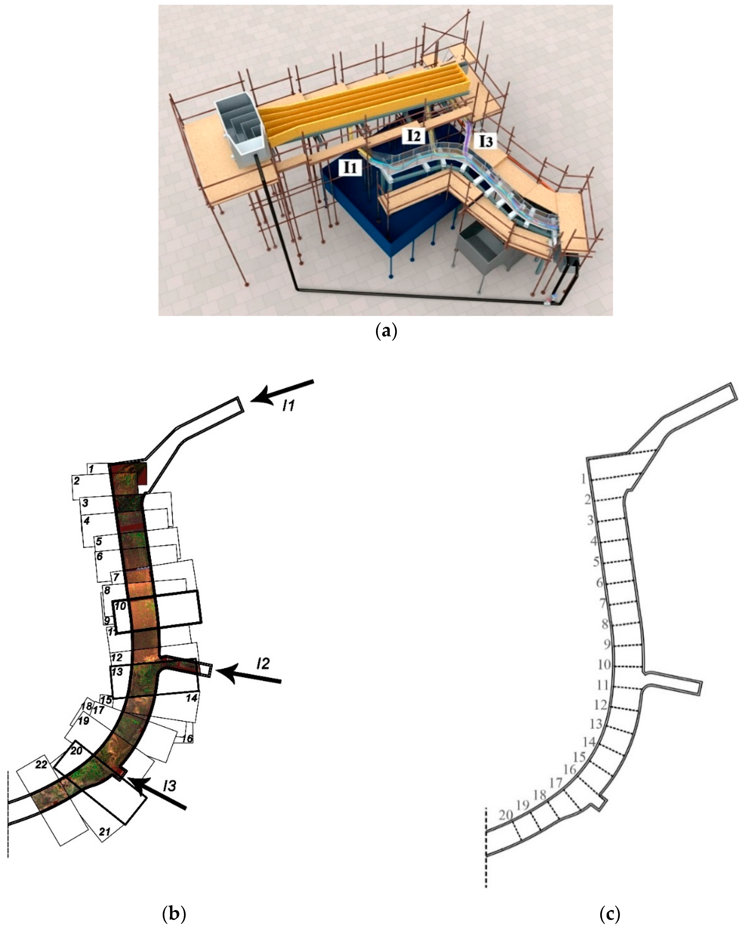
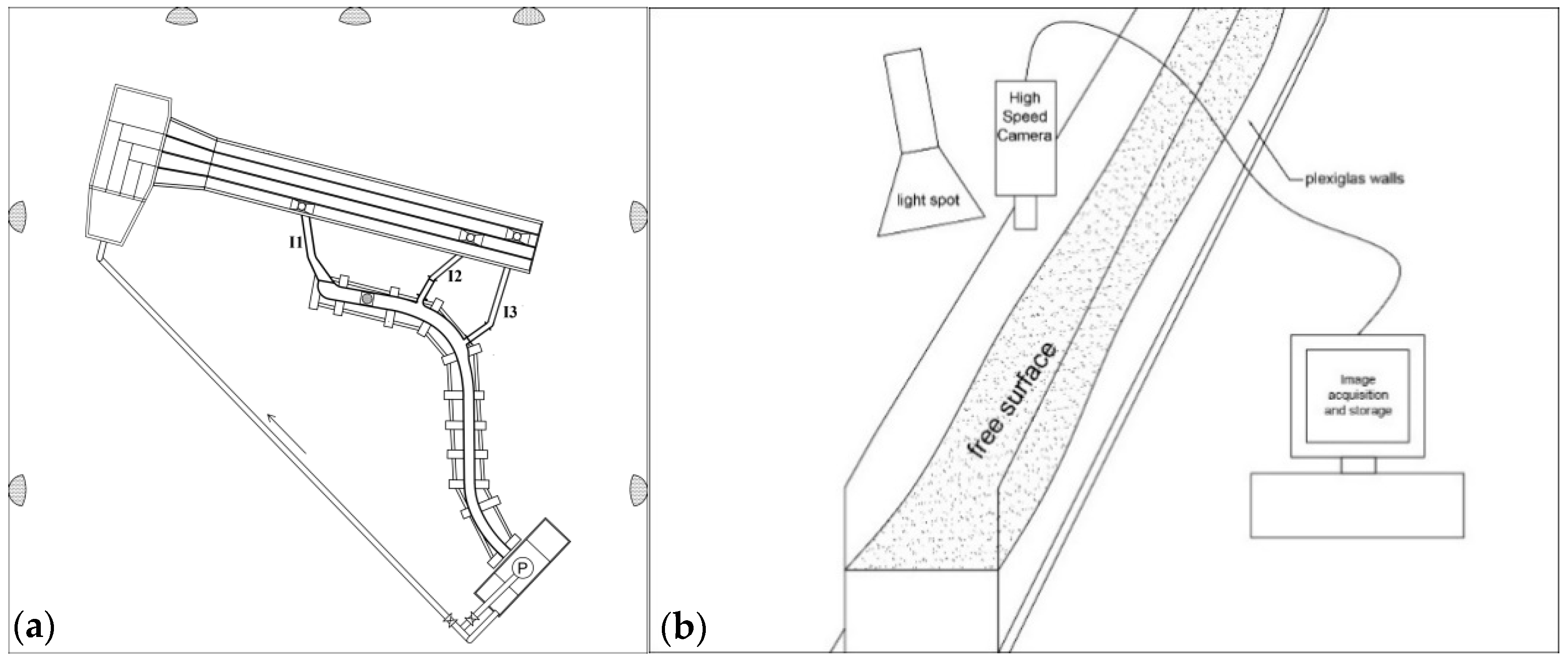
2.1. Experimental Apparatus and Conditions

An experimental program has been recently conducted at the Hydraulic laboratory of the Department of Civil, Environmental, Aerospace and of Materials Engineering (DICAM)—University of Palermo (Italy) in order to analyze the propagation phenomenon of hyper-concentrated flow in a defense channel. A series of experiments was conducted in a 1:35 scale flume reproducing the defence channel under construction in a small urban area of Messina’s territory (Italy). Such a defence channel was designed after a huge rainfall in 2009 that mobilized large amount of sediments causing damages and death. The experimental apparatus is shown in Figure 1. As Figure 1 shows, the main channel includes three inflow channels denominated respectively as I1, I2, and I3. The bed is concrete and the channel’s walls are Plexiglas strips. The channel’s width is equal to 23 cm in the reach between section 1 and section 15 (see Figure 1c) and it is equal to 17 cm from section 18 until the last section of the channel.
During the experiments, the water–sediment mixture was recycled through a pump located in the downstream reservoir. The water–sediment mixture was obtained by using field sediments (medium sediment diameter d50 = 2 mm) and it includes sediment particles with diameter ranging between 1 × 10⁻¹ mm and 2 × 10⁻³ mm. The sediment concentration varied in the range 10%–50%. During the experiments, the inflow discharge was measured both upstream of the inflow channels and in peculiar sections (sections 4, 5, 11, 12 of Figure 1c) along the channel by using the ultrasonic instrument Mainstream EH7000 (by Endress + Hauser S.p.a.). In the present work, attention is focused on experimental runs conducted with sediment concentration of around 50% and values of the discharge at inflow channels respectively equal to QI1 = 0.004 m3/s, QI2 = 0.00135 m3/s, QI3 = 0.00174 m3/s.

2.2. Acquisition and Processing Methodology

The PIV technique consists of four steps: (1) recording images; (2) pre-processing, which allows the improvement of the information to be taken from the images; (3) evaluation, which allows the application of the cross-correlation algorithm; (4) post-processing, which allows the interpretation of results. The processing procedure was carried out by the help of the PivLab algorithm in Matlab. A high speed camera (AOS Technology AG) was used to record the flow motion. In order to reproduce conditions similar to those in field, the images were acquired either by natural lighting or by using halogen lamps opportunely positioned to obtain a homogenous illumination [35,39]. Preliminary runs were conducted in order to set illumination conditions and to select the rate of the acquisition frequency as function of the camera’s characteristics and the number of images to cover the channel. During the preliminary runs, the streamwise velocity component was also measured at some control points opportunely selected along the channel by using an acoustic velocity profiler (DOP2000 by signal processing s.r.l.). Finally, the illumination system consisted of 7 halogen lamps distributed along the boundaries of the channel’s area and positioned above the channel at an adequate height so as to have a homogeneous and diffused illumination on the surface without shadows or light reflections [40]; another halogen lamp (type ARRI 2000W with filter lens and electric ballast) centered upon the channel and collocated on the top of the camera was also used (see Figure 2).
As described in detail in [38], a rate of 600 frames per second with image resolution of 640 × 240 pixels (px) was chosen and 22 images were considered to cover the examined channel reach (see Figure 1b). In order to maintain a constant optical cone width, the camera was placed on a plane parallel to the channel’s bed and centered upon the channel at a constant distance of 1.5 m from the bed. Furthermore, both target points and reference meters were positioned on the bed and on the channel’s walls for the geometrical correction of the images. The target points and the reference meters were used to apply the calibration and rectification toolbox for MATLAB and to calibrate the length scale of the images. It was estimated that 1 px 1.2 mm.
During the experimental run, the particles of the water–sediment mixture were considered as natural tracers for the PIV analysis. For each image, a sequence of frames was recorded by means of the high-speed camera. The number of recorded frames per image ranged between 4800 and 6000. Then, artificial tracers consisting of insoluble and floating wooden particles of 10 mm in diameter and 3 mm high were released into the hyper-concentrated flow. The artificial particles were painted with yellow phosphorescent color in order to ensure their visibility. Once these particles were released in the hyper-concentrated flow, sequences of images were again recorded at constant time intervals by means of the high-speed camera. This allowed us to track the particles trajectories at different times. The information obtained by using the artificial seeding were used in the pre-processing step in order to eliminate some errors before correlation process, to remove peculiar anomalies from the considered dataset [32] and to calibrate the pre-processing camera settings [34,35]. For the calibration, the values of flow velocity components previously measured by using the acoustic velocity profiler during the preliminary runs were also used. A high-pass filter was applied to remove the background signal [36] and the FFT window deformation was considered. For each image, the region of interest (ROI) was identified by excluding the pixels external to the flow field domain.
To apply the PIV method, each frame was thought as an independent sample of the velocity field and the statistical sampling theory was applied. According to previous works [7,31], the most probable displacement of a group of particles travelling on a straight line between two consecutive images was determined by applying the spatial cross-correlation method [41]. Each pair of frames was cross-correlated in order to obtain the most probable particles displacement in small sub-images (called as interrogation areas, IA). The correlation was operated between the interrogation area centered on a point aij in the first image and the interrogation area centered on a point bij in the second image recorded with a time δt as [30]:
C ( m , n ) = i j I A 1 ( i , j ) I A 2 ( i m , j n )
where IA1 and IA2 are, respectively, the interrogation areas in the first and in second image of a single exposed image pairs. The maximum peak location in C(m,n) indicates the particle displacement. The velocity vectors are derived from these displacements by dividing them by δt.
This procedure was iteratively applied for the whole image by the help of the PivLab algorithm in Matlab. The PivLab algorithm considers pairs of images temporally consecutive by recognizing the lighting intensity reflected by each particle into the flow over time. The cross-correlation is estimated by the fast Fourier transform (FFT) in multi-pass correlation mode [35]. In particular four passes have been used. This means that the estimation of particle’s displacement depends both on the number of frames considered and on the resolution of the recorded images.
Finally, the velocity vectors were estimated in nodes of a regular rectangular mesh, identified in the ROI of each image, whose size depends on the spatial resolution (dimension) of the interrogation area (IA).

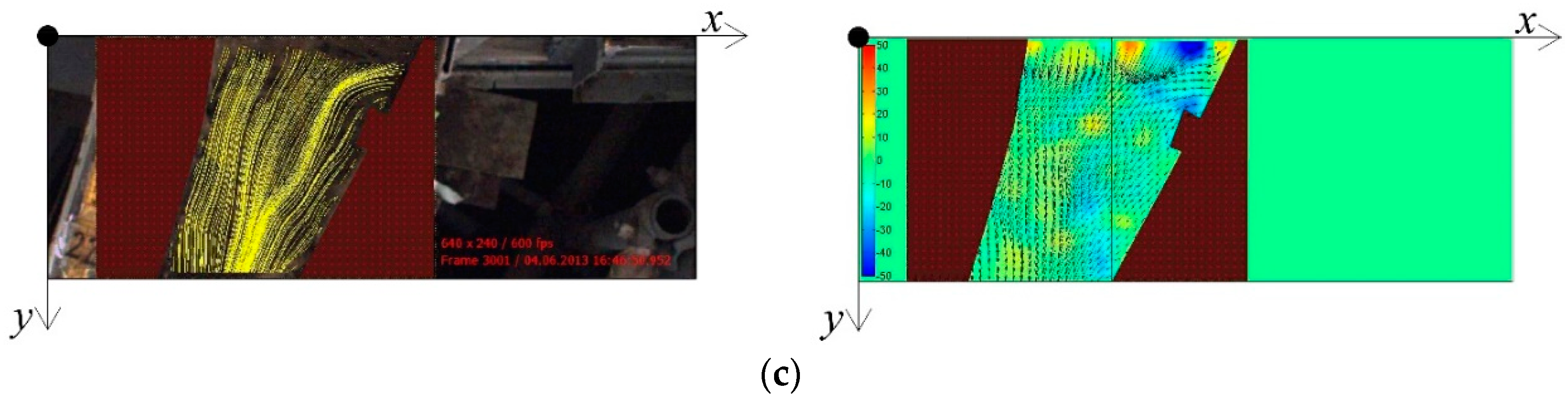
2.3. Surface Velocity Estimation by PIV Method

For each pair of frames, and thus for each corresponding instant tf, the flow velocity components [vx(tf) and vy(tf)] with respect the orthogonal local reference system (x, y), were determined with the PivLab Tool, as described in the previous Section 2.2. The application of the digital procedure allowed us to estimate, for each image, the distribution of the surface velocity vectors, the stream lines and the vorticity patterns at each time tf. As an example, Figure 3 reports the streamlines superimposed over the images and the velocity vectors superimposed over the vorticity contour maps at time tf = 5 s for images 10, 13, and 20.
For simplicity of exposition, these images have been selected to explain some of the obtained results because they are characterized by equal number of recorded frames and they are located in peculiar positions along the channel. In fact (see Figure 1b), image 10 is located along the straight reach downstream of the inflow I1, images 13 and 20 are located slightly downstream of inflow I2 and inflow I3, respectively; both the images 13 and 20 refer to curved channel stretches and the image 20 includes also the reach characterized by variable width. From Figure 3 it can be observed that the flow field estimated in sections 13 and 20 reveal the effect of confluence of the inflows I2 and I3 and free surface perturbations generated by turbulence eddies forming downstream the confluences occur. It should be noted that the velocity values reported in Figure 3 have been estimated in 1160 nodes/frame.
In the present work, interest is especially devoted to the time-averaged velocity. Thus, by using the time-series of vx(tf) and vy(tf), the corresponding time-averaged components ( v x ¯ ,   v y ¯ ) were determined for each node of the regular mesh identified as a function of the selected spatial resolution of the interrogation area. Then, the resultant time-averaged velocity of intensity v ¯ = v ¯ x 2 + v ¯ y 2 was estimated.

3. Results and Discussion

3.1. Estimation Error

From the “Introduction” and the results reported in previous works [34,35], it is clear that both the number of frames (which depends on the acquisition time selected) and the dimension of the interrogation area (on which the extension of the data sample depends) could influence the accuracy of the results. The measurement points are nodes of a regular mesh whose dimension depends on the dimension of the interrogation area and a high dimension of data sample could determine modeling processes too much time-consuming.
In order to perform the sensitivity analysis of the estimated surface velocity values to the number of pairs of frames, for all the recorded images, the velocity components vx(tf) and vy(tf) have been calculated in each node of the rectangular mesh, corresponding to a fixed dimension of the interrogation area, by considering six values of the total number of pairs of frames (i.e., of time instants) to be processed (n1 = 100, n2 = 500, n3 = 1000, n4 = 1500, n5 = 2000, n6 = 2400). The standard deviation (estimation error) of the velocity components has been determined for each i-th node of the mesh as:
σ n j i = j = 1 , n j ( p i , j p ¯ n j , i ) 2 n j   i   =   1 , ,   N   n j   =   100 ,   500 ,   1000 ,   1500 ,   2000 ,   2400
where pi,j and p ¯ n j , i are, respectively, the examined component p [p = v x ( t f ) , v y ( t f ) ] and the corresponding time-averaged value, N is the number of nodes. From the error theory [42], the measured averaged value of the examined velocity component p falls in the range p ¯ n j , i ± σ n j , i and the uncertainty in averaging the component p can be estimated as σE = σ n j , i / n j [42].
Figure 4 reports, for each component p, the highest value of the estimation error obtained by Equation (1) for each n j . It can be observed that, especially for the component p = v x ( t f ) , σ n j , i tends to decrease as the number n j increases; for n j > 1200 it assumes the lower values. Thus, the maximum value of the uncertainty σE in averaging the component p is obtained for n j = 100. In this case, it has been estimated that the uncertainty σE is less than 2.4% in the x direction and less than 4% in the y direction. For n j > 1200 the uncertainty σE becomes less than 1% in both the directions x and y. This means that a large sample size is necessary to obtain the same uncertainty in averaging the component p.
The deviation of the time-averaged velocity components, estimated for n j = 100, 500, 1000, 1500, 2000, from those evaluated for the highest number values of the total number of pairs of frames ( n j = 2400) has been obtained as:
σ n j ( p ¯ ) = i = 1 , N ( p ¯ n j , i p ¯ 2400 , i ) 2 N  
Figure 5 reports the estimated values of σ n j ( p ¯ ) against n j . From this figure it can be observed that σ n j ( p ¯ ) exponentially decreases as n j increases. Thus, for the examined velocity range, low and almost constant values of σ n j ( p ¯ ) are obtained for n j ≥ 1200, i.e., for a number of processed frames equal to or greater than half of the available number of pair of frames.
This behavior can be also observed from Figure 6 where the values of the time-averaged velocity components ( p ¯ = v x ¯ and p ¯ = v y ¯ ) estimated for n j = 100, 500, 1000, 1500, 2000, have been compared with those evaluated for n j = 2400. It can be seen that for all the considered images, and for both the velocity components, the points well fit the bisector line when n j > 1000.
Then, the sensitivity of surface velocity to the dimension of the interrogation area has been performed. The values of the component p ¯ have been estimated by considering different values of the interrogation area (IAk). In this case, it has been assumed a constant value n j = 2400. According to the literature [30], in order to keep the background noise in the correlation matrix low [42,43], the interrogation area was reduced in such a way as to obtain a minimum size of the interrogation area equal to one quarter of the initial size. This is in accordance with literature [42,43,44] which shows that the size of the interrogation area should be not less than 4 times of the maximum displacement. Thus, the size of the interrogation area of the first pass in the processing PivLab code was defined taking into account that the value of the maximum displacement lmax = Umax * dt (where Umax is the maximum measurable velocity and dt is the time step). The minimum size of the interrogation area was assumed equal to 8 × 8 pixels that is greater than 4 * lmax = 5.6 pixels. The maximum size of the interrogation area was determined on the basis of the ROI dimension in the PivLab code.
Thus, the sensitivity analysis has been conducted for five (k = 5) values of the spatial resolution of the interrogation area: IA1 = 32 px; IA2 = 24 px; IA3 = 16 px; IA4 = 12 px; IA5 = 8 px. It is clear that as the size of IAk decreases, the number of nodes Nk of the regular mesh increases. But, it should be considered that a high number of nodes determines modeling processes too much time-consuming.
Figure 7 plots, for all the images, the percent area IAk% against of the number of nodes Nk. Figure 7 indicates that the number of nodes increases with a logarithm law as the percent area decreases. Thus, a reduction of the interrogation area implies a remarkable increase of the number of nodes.
For each IAk, the cross-correlation has been determined with the PivLab tool and the velocity components vx(tf) and vy(tf) have been estimated in each node of the corresponding rectangular mesh. Then, the estimation error of the velocity values has been determined as:
σ i , k ( p ¯ ) = k ( p i , k p ¯ i , k ) 2 N k       =   1 , ,   N k   k   =   1 , ,   5
where Nk indicates the number of nodes corresponding to the k-th interrogation area, IAk. Figure 8 reports the highest value, σ k ( p ¯ ) , of the estimation error obtained varying the interrogation area IAk.
From Figure 8 it can be seen that σ k ( p ¯ ) tends to decrease as the size of the interrogation area increases until that it assumes the lower values for 16 px < IAk < 20 px; then it increases as the size of the interrogation area increases. It should be noted that for IA3 = 16 px the size of the interrogation area is reduced of one half compared to the original size.
Thus, the values of each time-averaged velocity component, p ¯ , estimated for the interrogation areas corresponding to k = 1, 2, 4 and 5 have been compared with those evaluated by assuming k = 3. This comparison is reported in Figure 9 which shows that for k > 2 the points tend to arrange around the bisector line, for k ≤ 2 they tend to move away from the bisector line. This behavior suggests that, for the examined case, a reduction of the size of interrogation area of one half compared with the initial size represents a good compromise between the extension of the data sample and the accurate estimation of flow velocity. This result could also be consistent with previous works [45] identifying a limit of the maximum recoverable spatial displacement in any sampling directions to half the window size in that direction.
Then, in order to verify the reliability of the estimated velocity measurements along the channel, the flux of mass in adjoining regions of consecutive images was also verified. As an example, Figure 10 reports the comparison between the profiles of the specific longitudinal, mx/ρ = htr v x ¯ (htr = local water depth), and transversal, my/ρ = htr v y ¯ , fluxes of mass estimated along two adjacent sections. Figure 10 shows that the profiles of the specific flux of mass compare well both in longitudinal and in transversal directions.

3.2. Discharge Estimation

Based on the results presented in the previous section, the discharge has been estimated by assuming IA3 = 16 px and n j = 1500 and the surface velocity vectors have been determined, as explained in Section 2.3, at nodes of the corresponding rectangular mesh.
Then, the transversal sections reported in Figure 1c have been considered and the time-averaged velocity components along the transversal and the stream-wise directions ( v t r ¯ and v l ¯ respectively—see Figure 11) have been estimated at the nodes included in each transversal section. For the aims of the present work, only the stream-wise velocity component v l ¯ has been considered.
According to reference [10], it has been assumed that the shape of the vertical profile of the stream-wise velocity component is the same at each node of the transversal section. Furthermore, from the literature it is clear that the depth-averaged velocity can be estimated as a function of the free-surface velocity [46] through a coefficient equal to 0.85, which is the value generally used with other measurement techniques. Recently, Termini and Moramarco [6] by applying the entropy-based approach, verified that the maximum velocity is linearly related to the mean flow velocity through a dimensionless parameter Φ(M) (M is the entropic parameter) which assumed a value of around 0.8 along the curved stretches of the channel. Other authors (see in [47]) found a value of such a coefficient equal to 0.9.
In the present work, by taking into account that the water depths are very low (order of magnitude of 1 cm) the difference between the depth-averaged and the surface velocities has been assumed almost null so that the coefficient has been assumed equal to 1. The discharge has been determined as the sum of the elementary stream-wise flux per unit time estimated as: q = v ^ l h t r t r ( t r = width of the elementary area in the transversal direction tr—see Figure 11). In Figure 12 the estimated values of the discharge (qe) have been compared with those measured (qm) in sections 4, 5, 11, 12. From the Section 2.1 it is clear that the value of flow discharge measured by the ultrasonic instrument at sections 4 and 5 is equal to QI1 = 0.004 m3/s and that measured at sections 11 and 12 is equal to QI1 + QI2 = 0.00537 m3/s. Furthermore, Table 1 reports the values of the normalized error in the discharge estimation:
σ q = q m q e q m  
Figure 11 shows that the points arrange around the line of perfect agreement demonstrating a good agreement between the estimated and the measured values of the discharge. From Table 1 it can be seen that the highest value of error is of 22.0 (%).

4. Conclusions

The present paper concerns the application of fully digital approach for estimating the surface velocity and the discharge. In particular, the efficiency of the procedure is investigated for two parameters: the number of frames to be processed and the size of the interrogation area to be correlated. The analysis has been carried out by the help of the PivLav tool in Matlab. The results obtained from the presented analysis can be summarized as follows:
-
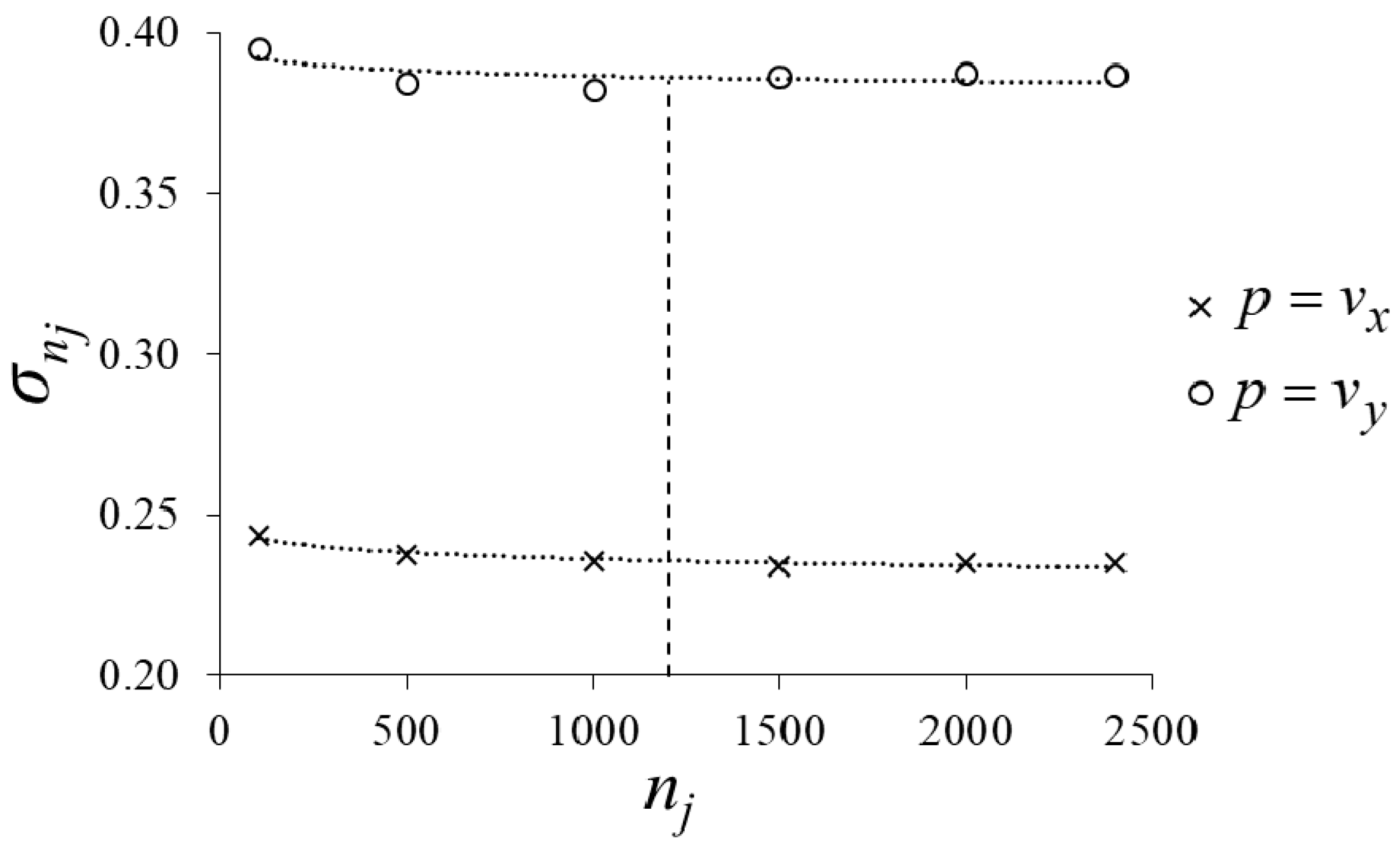
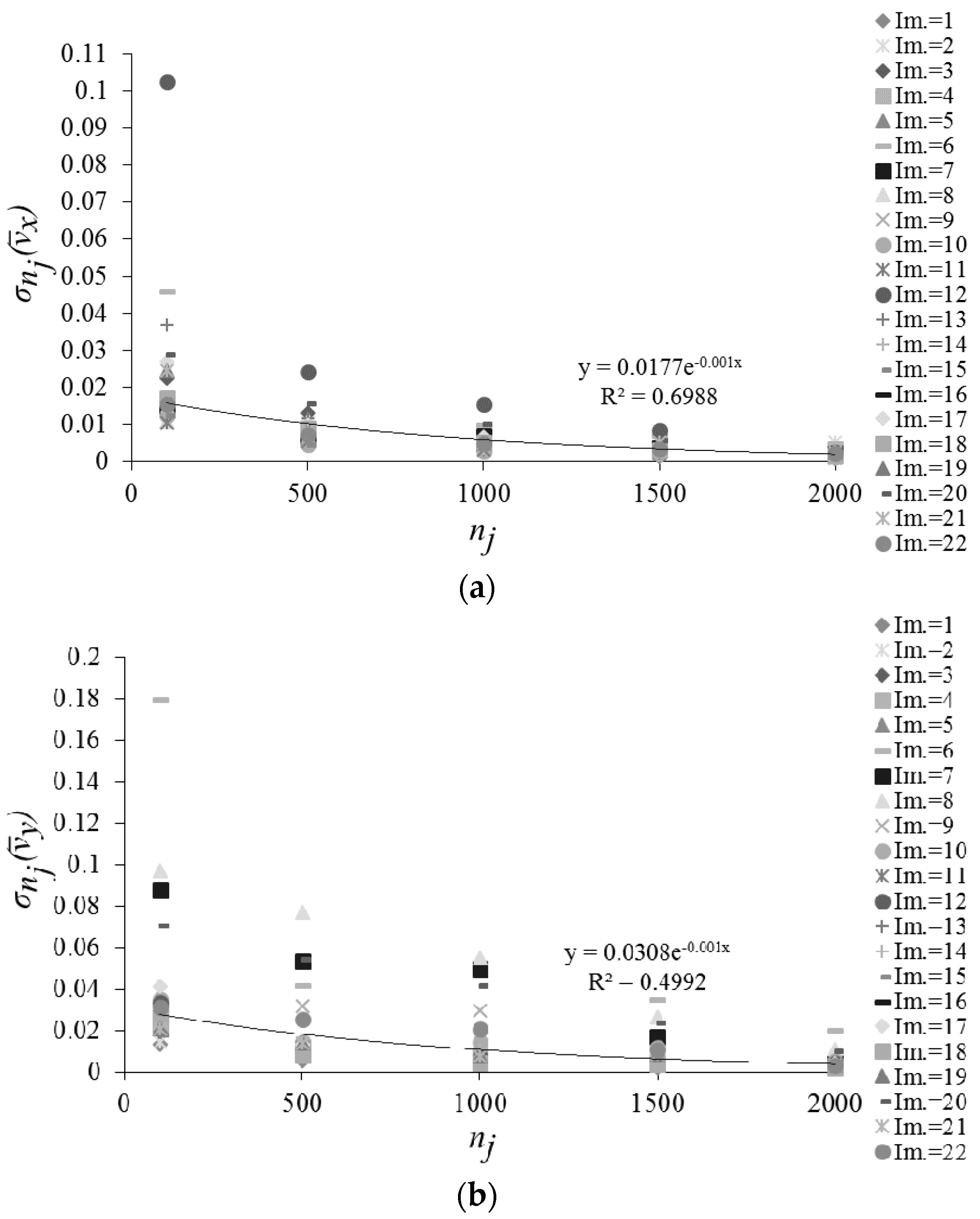
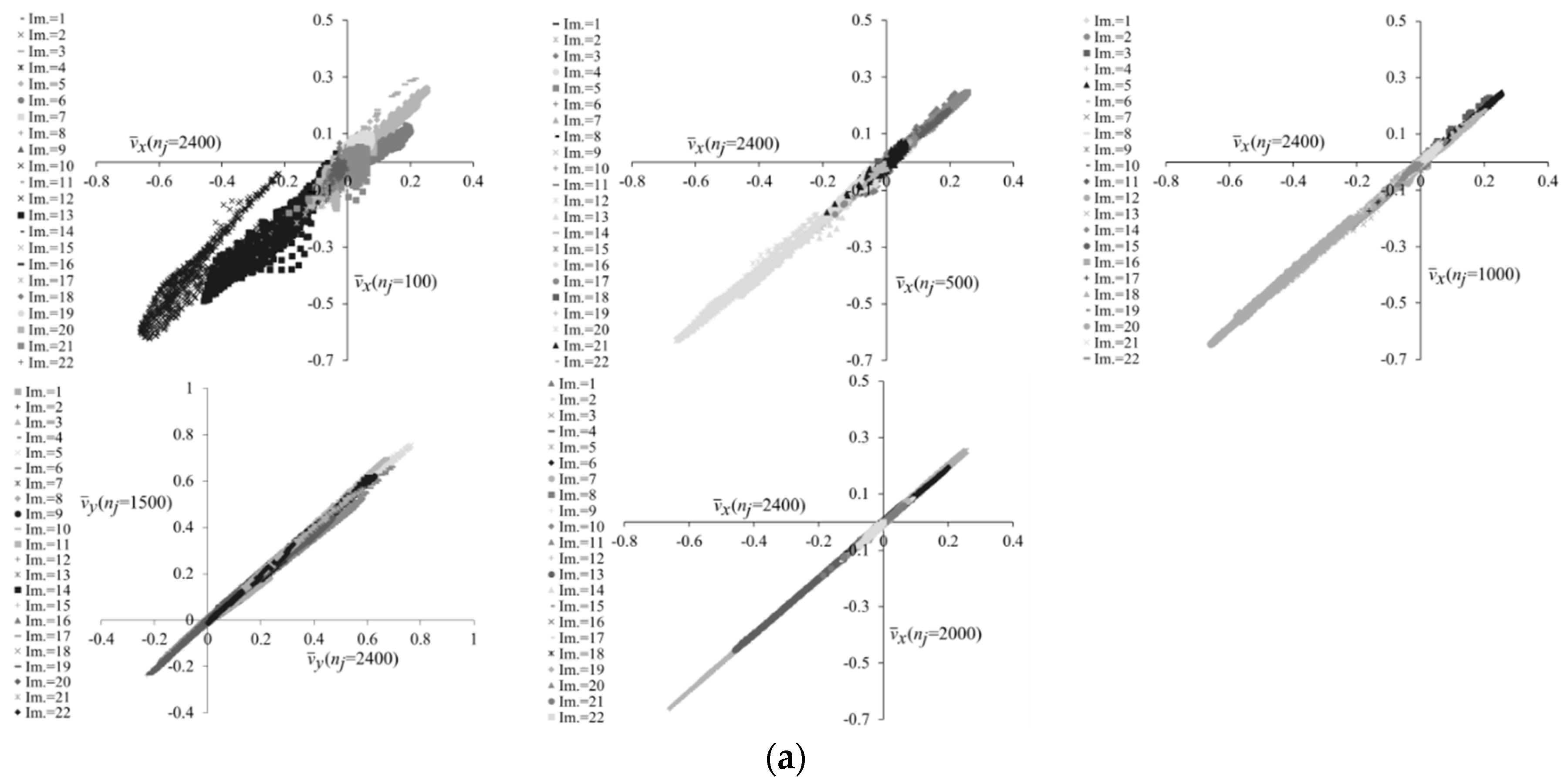
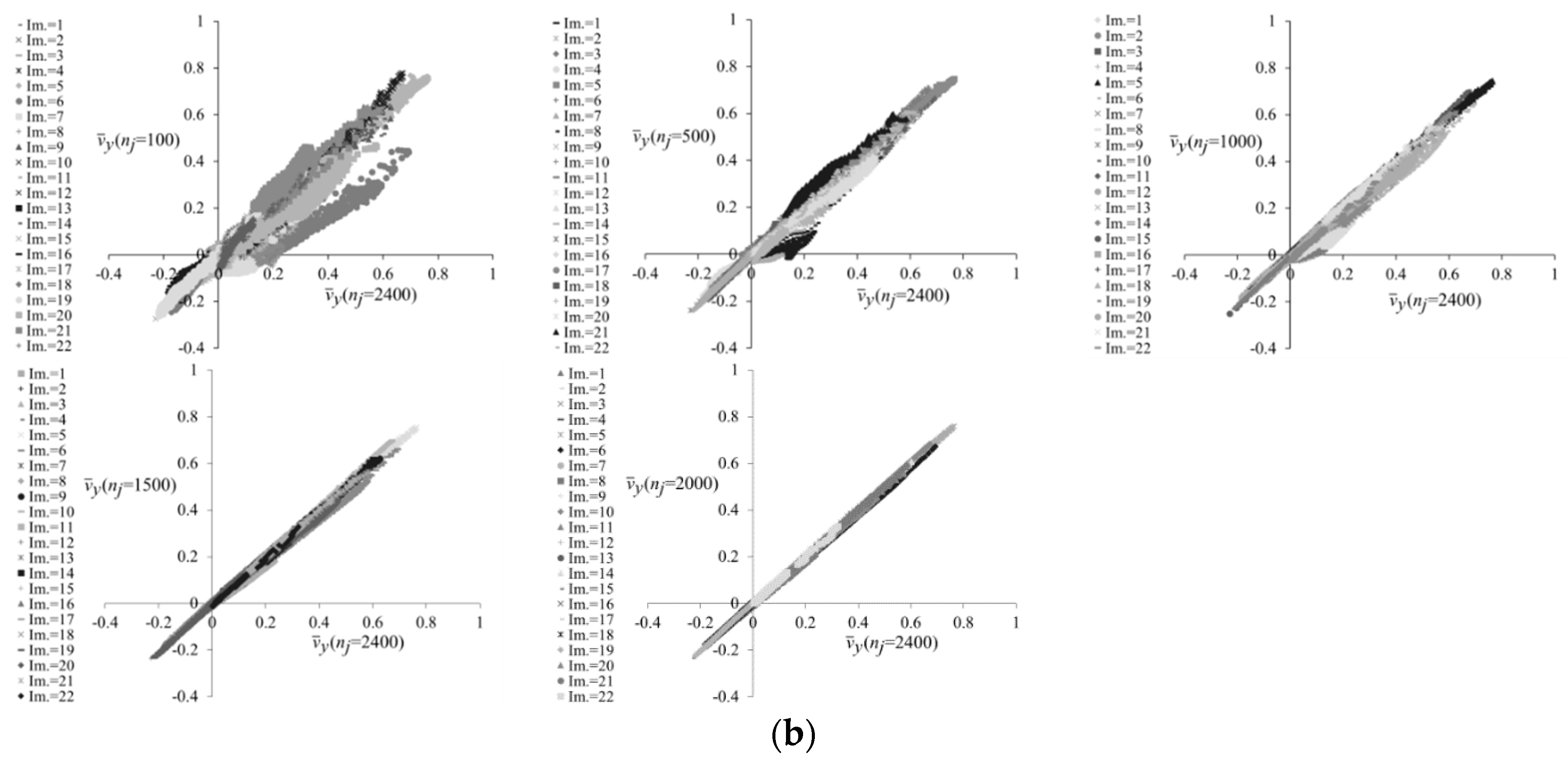
the estimation error of the surface velocity decreases as the number of pairs of frames increases. In particular, for the examined case, the estimation error assumes a low and an almost constant value as the number of processed pairs of frames is greater than 1200 (i.e., equal to or greater than half of the available pairs of frames);
-
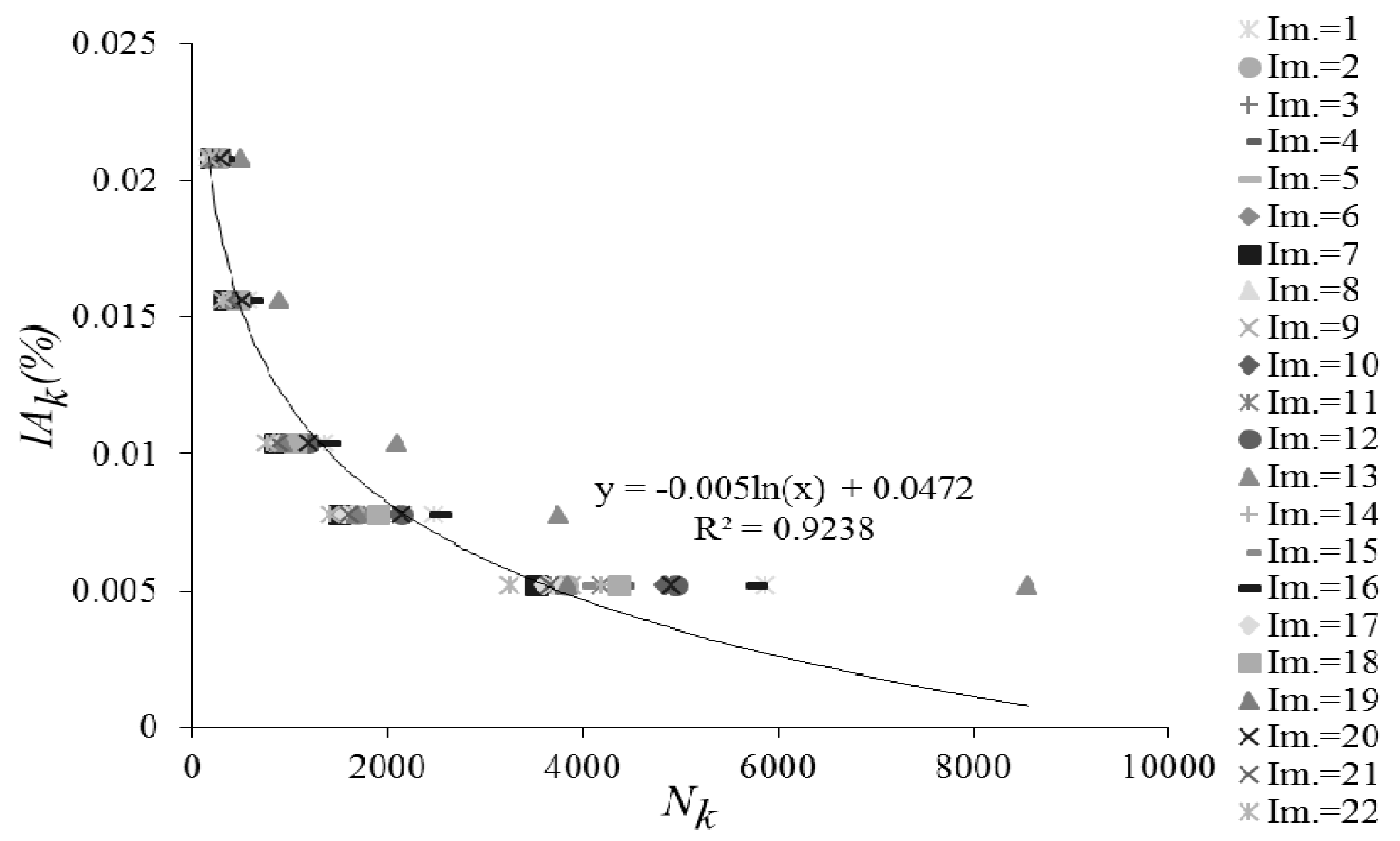
the size of the interrogation area plays an important role in the surface velocity estimation. It has been verified that the number of nodes increases with a logarithm law as the interrogation area decreases. But, the problem is that a high extension of the data sample makes the modeling process too time-consuming. As result of the sensitivity analysis of the surface velocity to the size of the interrogation area, it has been found that a reduction of the size of the interrogation area of about one half compared to the initial size represents a good compromise between the extension of the data sample and the accurate estimation of flow velocity;
-
the application of the PIV method has provided detailed information of the spatial distributions of instantaneous surface velocity vectors and of free surface perturbations related to the formation of large eddies downstream of the confluences. Furthermore, by using the spatial distributions of time-averaged surface velocity obtained by applying the PIV analysis, the values of the discharge in peculiar sections along the channel have been estimated. The good agreement between the estimated values of the discharge and the measured ones has demonstrated the ability of the digital image-technique for remote monitoring of free-surface velocity and discharge measurement.
It should be noted that the presented results have been obtained in the controlled environment of a laboratory. This could suggest that the errors in the field might outweigh the errors tested in this study. Despite this limitation, the study allows us to gain insight into the applicability conditions of the PIV method for estimating the free surface velocity and flow discharge in hyper-concentrated flows. The obtained results could also be used for improving the application of the image-technique for monitoring activities of velocity in natural rivers, especially for velocity ranges similar to that analyzed in the present work.

Author Contributions

D.T. conceived and designed the work; D.T. and A.D.C. performed the experiments; D.T. and A.D.C. analyzed the data; D.T. and A.D.C. wrote the paper; A.D.C. improved the final editing of the figures; D.T. performed the final correction and editing of the work.”

Funding

This research received no external funding

Acknowledgments

The experimental apparatus in Palermo has been supported by the Regional Department DRPC and GC of Messina (Sicily).

Conflicts of Interest

The authors declare no conflict of interest

References

  1. Brown, R.A.; Pasternack, G.B. Hydrologic and topographic variability modulate channel change in mountain rivers. J. Hydrol. 2014, 510, 551–564. [Google Scholar] [CrossRef] [Green Version]
  2. Sukhodolov, A.; Sukhodolova, T. Evolution of mixing layers in turbulent flow over submersed vegetation: Field experiments and measurement study. In Proceedings of the International Congress Riverflow, Lisbon, Portugal, 6–8 September 2006. [Google Scholar]
  3. Rehmel, M. Application of Acoustic Doppler Velocimeters for Streamflow Measurements. J. Hydraul. Eng.-ASCE 2007, 133, 1433–1438. [Google Scholar] [CrossRef]
  4. Moramarco, T.; Singh, V.P. Formulation of the entropy parameter based on hydraulic and geometric characteristics of river cross sections. J. Hydrol. Eng. 2010, 15, 852–858. [Google Scholar] [CrossRef]
  5. Moramarco, T.; Termini, D. Entropic approach to estimate the mean flow velocity: Experimental investigation in laboratory flumes. Environ. Fluid Mech. 2015, 15, 1163–1179. [Google Scholar] [CrossRef]
  6. Termini, D.; Moramarco, T. Application of entropic approach to estimate the mean flow velocity and manning roughness coefficient in a high-curvature flume. Hydrol. Res. 2016, 48, 634–645. [Google Scholar] [CrossRef]
  7. Schabacker, J.; Bölcs, A. Investigation of Turbulent Flow by means of the PIV Method. In Proceedings of the 13th Symposium on Measuring Techniques for Transonic and Supersonic Flows in Cascades and Turbomachines, LTT-CONF-1996-001, Iowa City, IA, USA, 11–14 July 1996. [Google Scholar]
  8. Jodeau, M.; Hauet, A.; Paquier, A.; Le Coz, J.; Dramais, G. Application and evaluation of LS-PIV technique for the monitoring of river surface in high flow conditions. Flow Meas. Instrum. 2008, 19, 117–127. [Google Scholar] [CrossRef] [Green Version]
  9. Hauet, A.; Creutin, J.D.; Belleudy, P.; Muste, M.; Krajewski, W. Discharge measurement using Large Scale PIV under varied flow conditions—Recent results, accuracy and perspectives. In Proceedings of the International Congress Riverflow, Lisbon, Portugal, 6–8 September 2006. [Google Scholar]
  10. Muste, M.; Fujita, I.; Hauet, A. Large-scale particle image velocimetry for measurements in riverine environments. Water Resour. Res. 2008, 44, 1–14. [Google Scholar] [CrossRef]
  11. Voulgaris, G.; Trowbridge, J.H. Evaluation of the acoustic doppler velocimeter (ADV) for turbulence measurements. J. Atmos. Ocean. Technol. 1998, 15, 272–289. [Google Scholar] [CrossRef]
  12. Pereira, F.; Gharib, M.; Dabiri, D.; Modarress, D. Defocusing DPIV: A 3-component 3-D DPIV measurement technique application to bubbly flows. Exp. Fluids 2000, 29, S78–S84. [Google Scholar] [CrossRef]
  13. García, C.; Cantero, M.; Niño, Y.; García, M. Turbulence Measurements with Acoustic Doppler Velocimeters. J. Hydraul. Eng.-ASCE 2005, 131, 1062–1073. [Google Scholar] [CrossRef]
  14. Sarno, L.; Papa, M.N.; Tai, Y.C.; Carravetta, A.; Martino, R. A reliable PIV approach for measuring velocity profiles of highly sheared granular flows. In Proceedings of the 7th International Conference on Engineering Mechanics, Structures, Engineering Geology. WSAS Conference, Salerno, Italy, 3–5 June 2014; pp. 134–141. [Google Scholar]
  15. Creutin, J.; Muste, M.; Bradley, A.; Kim, S.; Kruger, A. River gauging using PIV technique: A proof of concept experiment on the Iowa River. J. Hydrol. 2003, 277, 182–194. [Google Scholar] [CrossRef]
  16. Adrian, R.J. Twenty years of particle image velocimetry. Exp. Fluids 2005, 39, 159–169. [Google Scholar] [CrossRef] [Green Version]
  17. Medina, V.; Bateman, A. Debris flow entrainment experiments at UPC, interpretation and challenges. In Proceedings of the 7th International Conference on Engineering Mechanics, Structures, Engineering Geology, WSAS Conference, Salerno, Italy, 3–5 June 2014; pp. 38–44. [Google Scholar]
  18. Fujita, I.; Muste, M.; Kruger, A. Large-scale particle image velocimetry for flow analysis in hydraulic engineering applications. J. Hydraul. Res. 1998, 36, 397–414. [Google Scholar] [CrossRef]
  19. Rahimzadeh, H.; Fathi, N.; Assodeh, M.H. An Experimental Model of Flow Surface Patterns at Vertical Downward Intake with Numerical Validation. In Proceedings of the 2006 IASME/WSEAS International Conference on Water Resources. Hydraulics & Hydrology, Chalkida, Greece, 11–13 May 2006; pp. 111–118. [Google Scholar]
  20. Meselhe, E.; Peeva, T.; Muste, M. Large Scale Particle Image Velocimetry for Low Velocity and Shallow Water Flows. J. Hydraul. Eng.-ASCE 2004, 130, 937–940. [Google Scholar] [CrossRef]
  21. Lueptow, R.M.; Akonur, A.; Shinbrot, T. PIV for granular flows. Exp. Fluids 2000, 18, 183–186. [Google Scholar] [CrossRef]
  22. Eckart, W.; Gray, J.M.N.T.; Hutter, K. Particle Image Velocimetry (PIV) for Granular Avalanches on Inclined Planes; Hutter, K., Kirchner, N., Eds.; Springer: Berlin, Germany, 2003; pp. 195–218. [Google Scholar]
  23. Pudasaini, S.P.; Hsiau, S.S.; Wang, Y.; Hutter, K. Velocity measurements in dry granular avalanches using particle image velocimetry technique and comparison with theoretical predictions. Phys. Fluids 2005, 17, 093301. [Google Scholar] [CrossRef]
  24. Pudasaini, S.P.; Hutter, K.; Hsiau, S.S.; Tai, S.C.; Wang, Y.; Katzenbach, R. Rapid flow of dry granular materials down inclined chutes impinging on rigid walls. Phys. Fluids 2007, 19, 053302. [Google Scholar] [CrossRef]
  25. Sheng, L.T.; Kuo, C.Y.; Tai, Y.C.; Hsiau, S.S. Indirect measurements of streamwise solid fraction variations of granular flows accelerating down a smooth rectangular chute. Exp. Fluids 2011, 51, 1329. [Google Scholar] [CrossRef]
  26. Sarno, L.; Papa, M.N.; Villani, P.; Tai, Y.C. An optical method for measuring the near-wall volume fraction in granular dispersions. Granul. Matter 2016, 18, 80. [Google Scholar] [CrossRef]
  27. Sarno, L.; Carleo, L.; Papa, M.N.; Villani, P. Experimental Investigation on the Effects of the Fixed Boundaries in Channelized Dry Granular Flows. Rock Mech. Rock Eng. 2018, 51, 203–225. [Google Scholar] [CrossRef]
  28. Sarno, L.; Carravetta, A.; Tai, Y.C.; Martino, R.; Papa, M.N.; Kuo, C.Y. Measuring the velocity fields of granular flows–Employment of a multi-pass two-dimensional particle image velocimetry (2D-PIV) approach. Adv. Powder Technol. 2018. [Google Scholar] [CrossRef]
  29. Lauterborn, W.; Vogel, A. Modern Optical Techniques in Fluid Mechanics. Annu. Rev. Fluid. Mech. 1984, 16, 223–244. [Google Scholar] [CrossRef]
  30. Huang, H.; Dabiri, D.; Gharib, M. On errors of digital particle image velocimetry. Meas. Sci. Technol. 1997, 8, 1427–1440. [Google Scholar] [CrossRef] [Green Version]
  31. Huang, H.T.; Fiedler, H.E.; Wang, J.J. Limitation and Improvement of PIV. Exp. Fluids 1993, 15, 263–273. [Google Scholar] [CrossRef]
  32. Hart, D.P. Piv error correction. Exp. Fluids 2000, 29, 13–22. [Google Scholar] [CrossRef]
  33. Termini, D.; Di Leonardo, A. Propagation of Hyperconcentrated flows in protection channels around urban areas: Experimental investigation. In Urban and Urbanization, 1st ed.; St. Kliment Ohridski University Press: Sofia, Bulgaria, 2014; pp. 125–133. [Google Scholar]
  34. Termini, D.; Di Leonardo, A. Hyper-concentrated flow and surface velocity estimation: A study case. In Proceedings of the 8th International Conference on Environmental and Geological Science and Engineering. WSAS Conference, Salerno, Italy, 27–29 June 2015. [Google Scholar]
  35. Termini, D.; Di Leonardo, A. Digital image-based technique for monitoring surface velocity: Sensitivity analysis with processing parameters using data of a study case. In Proceedings of the Riverflow 2016, Iowa City, IA, USA, 27–29 July 2016. [Google Scholar]
  36. Thielicke, W.; Stamhuis, E.J. PIVlab–Towards User-friendly, Affordable and Accurate Digital Particle Image Velocimetry in MATLAB. J. Open Res. Softw. 2014, 2, e30. [Google Scholar] [CrossRef]
  37. Thielicke, W.; Stamhuis, E.J. PIVlab–Time-Resolved Digital Particle Image Velocimetry Tool for MATLAB (version: 1.43). 2014. Available online: http://dx.doi.org/10.6084/m9.figshare.1092508 (accessed on 2 August 2005).
  38. Thielicke, W. The Flapping Flight of Birds–Analysis and Application. [S.l.]: [S.n.]. Ph.D. Thesis, Rijksuniversiteit Groningen, Groningen, The Netherlands. Published in 2014. Available online: http://irs.ub.rug.nl/ppn/382783069 (accessed on 16 October 2018).
  39. Kantoush, S.A.; Schleiss, A.J.; Sumi, T.; Murasaki, M. LSPIV implementation for environmental flow in various laboratory and field cases. J. Hydro-Environ. Res. 2011, 5, 263–276. [Google Scholar] [CrossRef] [Green Version]
  40. Rowinski, P. Experimental Methods in Hydraulic Research; Springer: Berlin, Germany, 2011. [Google Scholar]
  41. Utami, T.; Blackwelder, R.F. A cross-correlation technique for velocity field extraction from particulate visualization. Exp. Fluids 1991, 10, 213–223. [Google Scholar] [CrossRef]
  42. Grossfield, A.; Zuckerman, D. Quantifying uncertainty and sampling quality in biomolecular simulations. Ann. Rep. Comput. Chem. 2009, 1, 23–48. [Google Scholar]
  43. Gonzales, R.; Wintz, P. Digital Image Processing; Longman Higher Education: Harlow, UK, 1997. [Google Scholar]
  44. Scarano, F.; Riethmuller, M.L. Iterative multigrid approach in PIV image processing with discrete window offset. Exp. Fluids 1999, 26, 514–523. [Google Scholar] [CrossRef]
  45. Willert, C.E.; Gharib, M. Digital particle image velocimetry. Exp. Fluids 1999, 10, 181–193. [Google Scholar] [CrossRef]
  46. Polatel, C. Indexing free-surface velocity: A prospect for remote discharge estimation. In Proceedings of the 31th Congress International International Association Hydraulic Engineering and Research, Seoul, Korea, 11–16 September 2005. [Google Scholar]
  47. Welber, M.; Le Coz, J.; Laronne, J.B.; Zolezzi, G.; Zamler, D.; Dramais, G.; Hauet, A.; Salvaro, M. Field assessment of noncontact stream gauging using portable surface velocity radars (SVR). Water Resour. Res. 2016, 52. [Google Scholar] [CrossRef]
Figure 1. Experimental apparatus: (a) Render; (b) Plane-view of the images covering the examined channel; (c) Examined transversal sections.
Geosciences 08 00383 g001
Figure 2. (a) Scheme of the halogen lamps’ locations; (b) Scheme of images acquisition system.
Geosciences 08 00383 g002
Figure 3. Streamlines superimposed over the images and velocity vectors superimposed over the vorticity (1/s) patterns: (a) Image 10; (b) Image 13; (c) Image 20.
Geosciences 08 00383 g003aGeosciences 08 00383 g003b
Figure 4. Highest value of estimation error σ n j (m/s).
Geosciences 08 00383 g004
Figure 5. Deviation σ n j ( p ¯ ) for all the examined images: (a) p ¯ = v x ¯ (m/s); (b) p ¯ = v y ¯ (m/s).
Geosciences 08 00383 g005
Figure 6. Comparison between the component p ¯ = ( v ¯ x ; v ¯ y ) estimated for n j = 100, 500, 1000, 1500, and 2000 and the corresponding value estimated for n j = 2400: (a) p ¯ = v ¯ x (m/s); (b) p ¯ = v ¯ y (m/s).
Geosciences 08 00383 g006aGeosciences 08 00383 g006b
Figure 7. Percent area of the interrogation area (IAk%) and the number of nodes.
Geosciences 08 00383 g007
Figure 8. Highest value of σ k ( p ¯ ) (m/s) against IAk.
Geosciences 08 00383 g008
Figure 9. Comparison between component p ¯ = ( v x ¯ , v y ¯ ) obtained for IA1, IA2, IA4, and IA5 with those obtained for IA3: (a) p ¯ = v x ¯ (m/s); (b) p ¯ = v y ¯ (m/s).
Geosciences 08 00383 g009aGeosciences 08 00383 g009b
Figure 10. Comparison of specific flux of mass between sections of adjacent images (sections 5 and 5a, distant 2 cm apart): (a) longitudinal direction; (b) transversal direction.
Geosciences 08 00383 g010
Figure 11. Geometrical scheme for the discharge estimation.
Geosciences 08 00383 g011
Figure 12. Comparison between the estimated and measured values of discharge (l/s).
Geosciences 08 00383 g012
Table 1. Error in discharge estimation.
Sectionσqqe (m3/s)
40.170.0035
50.220.0033
11−0.130.0061
12−0.180.0063

