Article

Paleoenvironment Variability during Termination I at the Reykjanes Ridge, North Atlantic

1
Shirshov Institute of Oceanology, Russian Academy of Sciences, Nahimovskiy prospekt 36, 117997 Moscow, Russia
2
National Centre for Antarctic and Ocean Research, Vasco-da-Gama, Goa 403 804, India
*
Author to whom correspondence should be addressed.
Geosciences 2018, 8(10), 375; https://doi.org/10.3390/geosciences8100375
Submission received: 5 August 2018 / Revised: 23 September 2018 / Accepted: 5 October 2018 / Published: 11 October 2018
(This article belongs to the Section Biogeosciences)

Abstract

:
The micropaleontological study (radiolarians and foraminifera) of the sediment core AMK-340, Reykjanes Ridge, North Atlantic, combined with the radiocarbon dating and oxygen and carbon isotopic record, provided data for the reconstruction of the summer paleotemperature across the upper 100 meters water depth range, and paleoenvironments during the Termination I in the age interval of 14.5–8 ka. The response of the main microfossil species to the paleoceanographic changes within the Bølling-Allerød (BA) warming, the Younger Dryas (YD) cold event and final transition to the warm Holocene, was different. The BA warming was well captured by the radiolarian and benthic foraminiferal records, but not the planktic one. The high abundances of the cold-water radiolarian species Amphimelissa setosa as a Greenland/Iceland Sea indicator marked a cooling at the end of the BA and at the start of the YD at 13.2–12.3 ka. The micropaleontological and isotopic data together with the paleotemperature estimates for the Reykjanes Ridge at 60°N document that, after the warm BA, the middle YD ca. 12.5–12.2 ka was the next significant step toward the Holocene warming. The start of the Holocene interglacial conditions was reflected in large representation of the microfossils being indicators of the open boreal North Atlantic environments indicating increasing warmth.

1. Introduction

Our study presents new North Atlantic paleoceanographic results over the last deglaciation, which was a time of abrupt climatic changes (general warming superimposed by sudden short glacial reversals). Atlantic thermohaline circulation or North Atlantic meridional overturning circulation (NAMOC) mediates the climate for the surrounding land and climatic connections between hemispheres [1]. The sea surface conditions in the North Atlantic significantly influence the major modes of regional atmospheric circulation (meridional or zonal) [2] causing warming or cooling episodes. Rapid changes in the NAMOC and on the North Atlantic surface during the last deglaciation have influenced changes of the climatic conditions (global warming, melt-water discharge from land ice, sea-ice distribution) [3]. Overpeck et al. [4] postulated an apparent synchroneity of the rapid climate events in the circum-North Atlantic during the last deglaciation, but called for new high-resolution studies to prove this.
We use the micropaleontological data from the sediment core AMK-340 (the Russian RV “Akademik Mstislav Keldysh” station 340), combined with the radiocarbon dated oxygen and carbon isotopic record, to estimate the sea subsurface summer temperature and to describe the paleoenvironmental changes during Termination I on the Reykjanes Ridge circa (ca.) 60° N. Late Quaternary paleoceanography of the subpolar to polar North Atlantic has been extensively documented, particularly using microfossils to provide sea surface estimates [5], and references therein). Our aim is to get additional quantitative information on sea subsurface temperature and compare it with the global and regional paleoclimatic archives. The approach is a reconstruction of the paleotemperature based on the factor analysis of the radiolarian and planktic foraminiferal data in the same samples. The radiolarian distribution and paleotemperature estimates based on the radiolarians (old “graphical” paleotemperature method, and method of spline interpolations as a modification of the Q-mode analysis) for the core AMK-340 was presented by Matul [6], and Matul and Yushina [7]. This paper uses an improved modern and core radiolarian database, newly constructed modern planktic foraminiferal database, a standard paleotemperature method of the Q-mode analysis and transfer functions realized as a software PanTool Box [8] and also involves unpublished data on the planktic and benthic foraminifera in the core.
The study area is located on the eastern margin of the Subpolar (Irminger) Gyre (Figure 1). The western branch of the Irminger Current split from the warm North Atlantic Current influences the Reykjanes Ridge oceanography [9]. Conversion of surface and warm to deep and cold waters by the Irminger Current, East Greenland Current, and also the Labrador Sea Water within the Irminger Gyre is unstable, exhibiting large interannual variability of the water flows at both the sea surface and deeper levels, thus complicating the local features of the NAMOC [10]. The average summer sea surface temperature at the location of the core AMK-340 is ca. 12 °C [11]. At the end of the last glacial period, before ca. 14 thousand years ago (ka), sea surface temperatures south of Iceland dropped to 0–2 °C [12]; therefore, prominent temperature and environmental changes within the transition from the last glacial to the Holocene interglacial on the Reykjanes Ridge occurred.

2. Material and Methods

The gravity core AMK-340 was obtained from the central area of the Reykjanes Ridge, North Atlantic (58°30.6′ N, 31°31.2′ W, water depth of 1689 m; core length of 387 cm) during the 4th cruise of the Russian RV “Akademik Mstislav Keldysh” in 1982 (Figure 1). The lithology of the core is composed of (1) 0 to 241 cm pelitic calcareous muds with CaCO3 content of 40–50%, (2) 241 to 307 cm pelitic weakly calcareous muds with CaCO3 content of 10–25%, (3) 307 to 387 cm pelitic muds with CaCO3 content of ≈10% alternated by the thin layers of the pelitic weakly siliceous muds. The lithology figure can be found in the publication of Matul [6]. In the paleoceanographic interpretation (see Results and Discussion section) we use the published paleotemperature, isotopic and micropaleontological data on the cores RAPiD-10-1P (62.9755° N, 17.5895° W, 1237 m water depth), RAPiD-12-1K (62.09° N, 17.82° W, 1938 m water depth), and RAPiD-15-4P (62.293° N, 17.134° W, 2133 m water depth) (Figure 1) [13,14].
The chronology of the core has been established from four AMS (Accelerator Mass Spectrometry) 14C-dated samples of the planktic foraminifera Neogloboquadrina (N.) pachyderma left coiled or sinistral (sin.) shells in the Leibniz Laboratory for Radiometric Dating and Stable Isotope Research at the Christian-Albrechts-University of Kiel, Germany (Table 1).
Radiocarbon ages were converted to calendar ones via the calibration program CALIB 7.1 using the MARINE13 scale (standard reservoir age correction R is 405 years with the regional ∆R of 85 ± 79 years) [16]. The age–depth plot is presented in Figure 2. We have no direct age dating of the core top, and tentatively assume the core top to be modern but nonetheless are aware of its older age. If we were to take into account the old radiocarbon data of the core sediments based on the total organic carbon [6], the calendar age of the AMK-340 sample 10–15 cm could be 1730 years, thus, the core top should be younger than 1 ka. Core AMK-340 spans the last ca. 14.5 kyr, which is the Holocene and the end of the last glacial period, including most of the deglacial warming. In the Results and Discussion section we concentrate on the paleoceanography of the Termination I as there is no appropriate age control of the upper core part. To identify the above-mentioned paleoclimatic intervals, we have used the standard ages of the Greenland stadials and interstadials recognized in the core, using the INTIMATE event stratigraphy [17]: start of the Bølling-Allerød (BA) warm interval is at ca. 14.7 ka, start of the Younger Dryas (YD) cold interval is at ca. 12.9 ka, and start of the Holocene warming is at ca. 11.7 ka. The average sedimentation rate of the core is ca. 26 cm·ky-1. The planktic foraminiferal species N. pachyderma (sin.) and Globigerina (G.) bulloides tests were picked out for the oxygen and carbon isotopic analysis in the Marine Stable Isotope Lab (MASTIL) of the National Centre of Antarctic and Ocean Research, Vasco-da-Gama, Goa, India. The size range of the planktic foraminiferal tests chosen is >100 μm. The external precisions of δ18O and δ13C analysis are ±0.15‰ and ±0.09‰, respectively (1σ standard deviation) obtained by repeatedly running NBS-19 (the reference isotopic standard material according the National Bureau of Standards of USA) as the Standard (n = 33). The δ18O and δ13C values are reported with respect to V-PDB (Vienna Pee Dee Belemnite).
We studied polycystine radiolarians (siliceous) and benthic and planktic foraminifera (calcareous) microorganisms in 37 sediment samples of 2-cm thickness each throughout the core, with a time resolution as high as 133 years.
For the radiolarian analysis, air-dried sediment samples of 1–2 g were boiled in a solution of 30% hydrogen peroxide and sodium pyrophosphate, and the carbonates were removed by adding a solution of 10% hydrochloric acid. The residue was washed through a 50 μm sieve. Then we subsampled a known aliquot with a pipette in order to later obtain the quantitative estimates and settled it on the cover glass and mounted on the slide in Canada balsam. As a rule, at least 250–300 radiolarians tests were counted under the transmitted light microscope at the ×300–600 magnification. Percentages of the radiolarian species and total radiolarian abundances as test·g−1 of bulk dry sediment were calculated.
For the foraminiferal analysis, air-dried sediment samples of available weight were washed through a 100 μm sieve. The dried fraction of >100 μm was thoroughly mixed and divided until the remaining split contained at least 300 tests. We identified and counted all components (mineral grains, planktic and benthic foraminifera) in this split, and, additionally, examined the whole fraction of >100 μm to find rare species that might be omitted from the split. The “foraminiferal number” (the number of shells larger than 100 μm per 1 g of dry sediment) and percentages of all planktic and benthic foraminiferal species were then calculated.
We found 25 benthic foraminiferal species in the core. The detailed study of the benthic microfauna from the core AMK-340 will be published later [18]. In the current paper, we present data on two benthic species that can be good indicators of the organic matter fluxes to the bottom: Cassidulina (C.) teretis and Globocassidulina (G.) subglobosa. C. teretis feeds on the bacteria from the soft, enriched by the organic matter sediments [19], G. subglobosa marks high spring phytodetrital fluxes [20]; therefore, we can use data on their quantity changes as possible indirect indication of the bioproductivity variations.
The paleotemperature was reconstructed by a method of Q-mode factor analysis and transfer functions. The PaleoTool Box software with its latest PC-version [8] provides the platform to make a statistical analysis of the micropaleontological data.
Transfer functions which allow paleotemperature estimates are based on the treatment of the modern micropaleontological datasets. The North Atlantic reference datasets used here consist of (1) 36 polycystine radiolarian species in 91 surface sediment samples from the area between 40 and 73° N [21], and (2) 23 planktic foraminiferal species in 237 surface sediment samples from the area between 40 and 80° N as a compilation from the Atlantic Ocean database of the Shirshov Institute of Oceanology, Moscow, Russia (134 stations from [22]) and World Ocean database (103 stations from [23]. Stations are presented in Figure 3. In the down-core record, we found no microfossil assemblages that are similar to the modern tropical/subtropical ones in the North Atlantic south of ca. 40° N. Therefore, we used stations from the areas north of this latitude. A temperature at the subsurface depth of 100 m is chosen as a basic parameter to be reconstructed for the interpretation because this depth can be assumed to represent the median level of the prevailed habitat of radiolarians [24] and planktic foraminifera [25]. In the North Atlantic, the highest abundances of the marine microzooplankton were found during May–September [26,27]; therefore, we analyze the summer temperature (July-August-September as the standard season in The World Ocean Atlas 2013 [11]). Most samples in our modern datasets on the radiolarians and planktic foraminiferas in the surface sediments were obtained from the end of 1950s to 1960–1970s, and the closest time interval with the averaged temperatures in the World Ocean Atlas 2013 [11] which we use is 1955–1964.
A comprehensive description of the PanTool Box application can be found in publications of Zielinski [28] and Zielinski et al. [29]. In the construction of the modern micropaleontological datasets, we follow recommendations of Imbrie and Kipp [30] that every microfossil species must have abundances >1–2% in one sample and occurs at least in 10 samples. Every radiolarian and planktic foraminiferal species from the modern datasets were found in the core. Geographical range of samples and species distribution from the modern datasets covers environments which occurred in the area of study during the Late Quaternary so that we do not expect the non-analogue situation. As Zielinski et al. [29] argued, the method of the Q-mode factor analysis works better than the modern analogues method with the regional database (in particular, in the cold-water areas), which is our case.

3. Results and Discussion

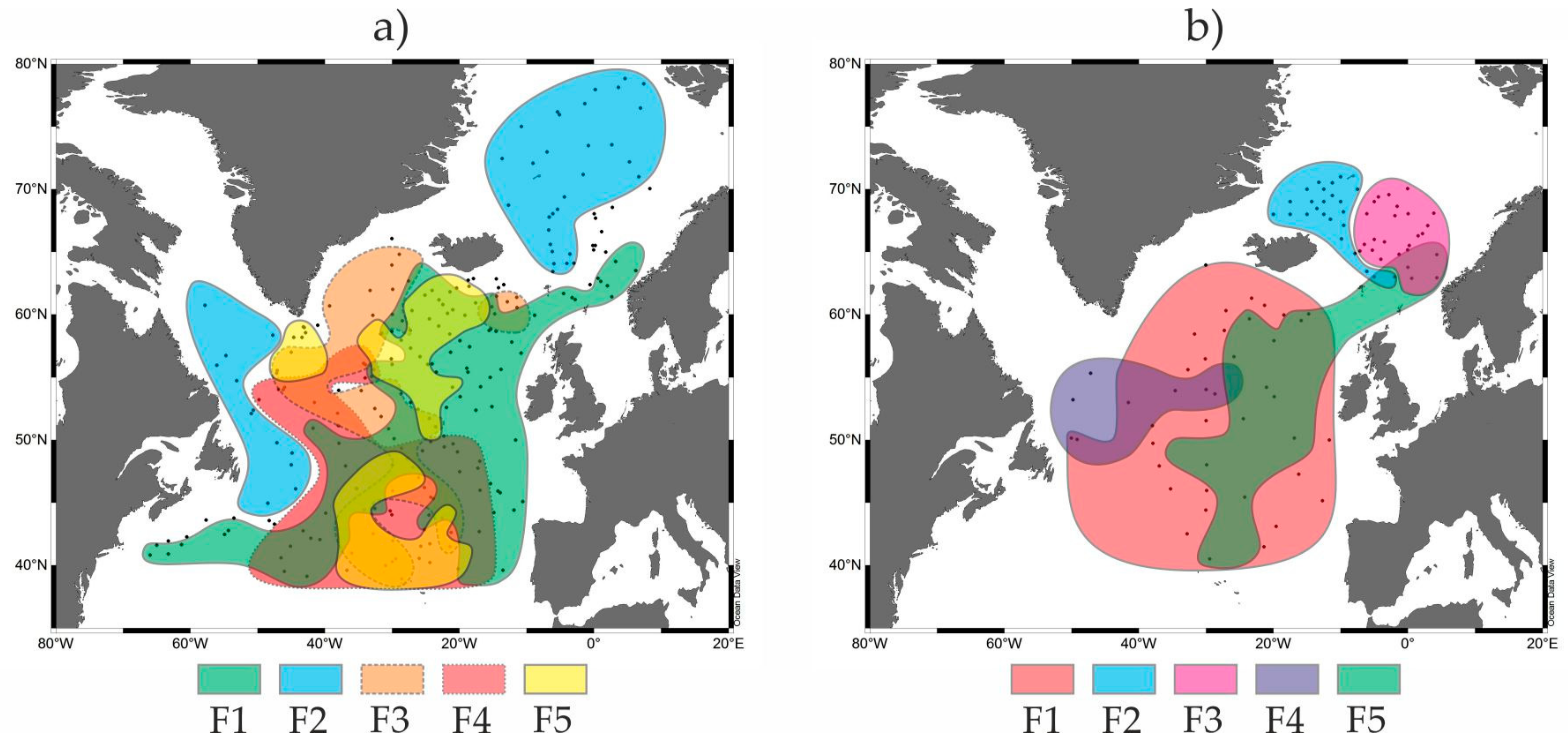
3.1. Modern Distribution of the Radiolarian and Planktic Foraminiferal Factors (=Assemblages) as a Base for the Paleotemperature Estimates

Factor analysis revealed 5 Factors (F) in the modern distribution of both planktic foraminifera (PF) and radiolarians (R) (Figure 3). They describe main oceanographic provinces within the studied area. Figures with detailed data on the radiolarian factor loadings and maps of the distribution of the main radiolarian species can be found in the publication of Matul and Mohan [21]. Similar figures on the planktic foraminiferal factor loadings and species distribution are in the Supplement to this paper.
Cold-water end-member is F2, with a leading foraminiferal species N. pachyderma (sin.) and radiolarian species Amphimelissa (A.) setosa. PF of F2 are typical for Greenland, Iceland, western and northern Norwegian, and Labrador Sea. Similarly, R of F2 occur in the southern Greenland and Iceland Seas but not in the Labrador Sea. The Polar/Arctic waters occupy these areas contacting with branches of the warmer Atlantic waters. Temperate-water F1 lies within the boreal open North Atlantic, where the dominant species are foraminiferal N. pachyderma (right-coiled or dextral (dex.) shells) and radiolarian Lithelius (L.) spiralis/minor group. Other factors give an additional view on the regional patterns of the microfauna in the open North Atlantic. PF of F3–F5 are distributed in the western, southern to southwestern, and central parts of the North Atlantic between latitudes of 40 and 65° N with leading species Turborotalia quinqueloba, G. bulloides, and Globigerinita glutinata, respectively. Radiolarian F4 (dominated by Artostrobium tumidulum and Phorticium clevei) and F5 (dominated by Lithomelissa setosa and Stylodictya validispina) indicate the mixing waters of the Labrador Sea and western North Atlantic, and eastern North Atlantic, respectively. Radiolarian F3 (dominated by Pseudodictyophimus gracilipes and Actinomma boreale/A. leptoderma group) is typical for the southern Norwegian Sea, an area of the active interaction of the warmer Atlantic and colder Arctic waters; it has no counterpart in the foraminiferal factor distribution.
Patterns in the distribution of Factors highlights the biogeography of various groups in the studied area, e.g., marine animals and plants [31], radiolarians [32], and planktic foraminifera [33], and references therein. More details on factors distribution is available in [34] for planktic foraminifera, and in [21,35] for radiolarians. In brief, the microfaunal assemblages that can be associated with factors are closely related to the different environments associated with the cold Polar/Arctic (the Nordic and Labrador Seas with temperatures of 0–5 °C on 100-m depth level) and warm temperate (the open North Atlantic with temperatures of 8–15 °C on 100-m depth level) water masses. This enable us to estimate, based on the transfer functions, the paleotemperature between the last glacial maximum 21 ka and the Holocene when the temperatures on sea-surface in the high latitudes and air temperatures in Greenland could increase at least on 3–6 °C and 15°C, respectively [36].

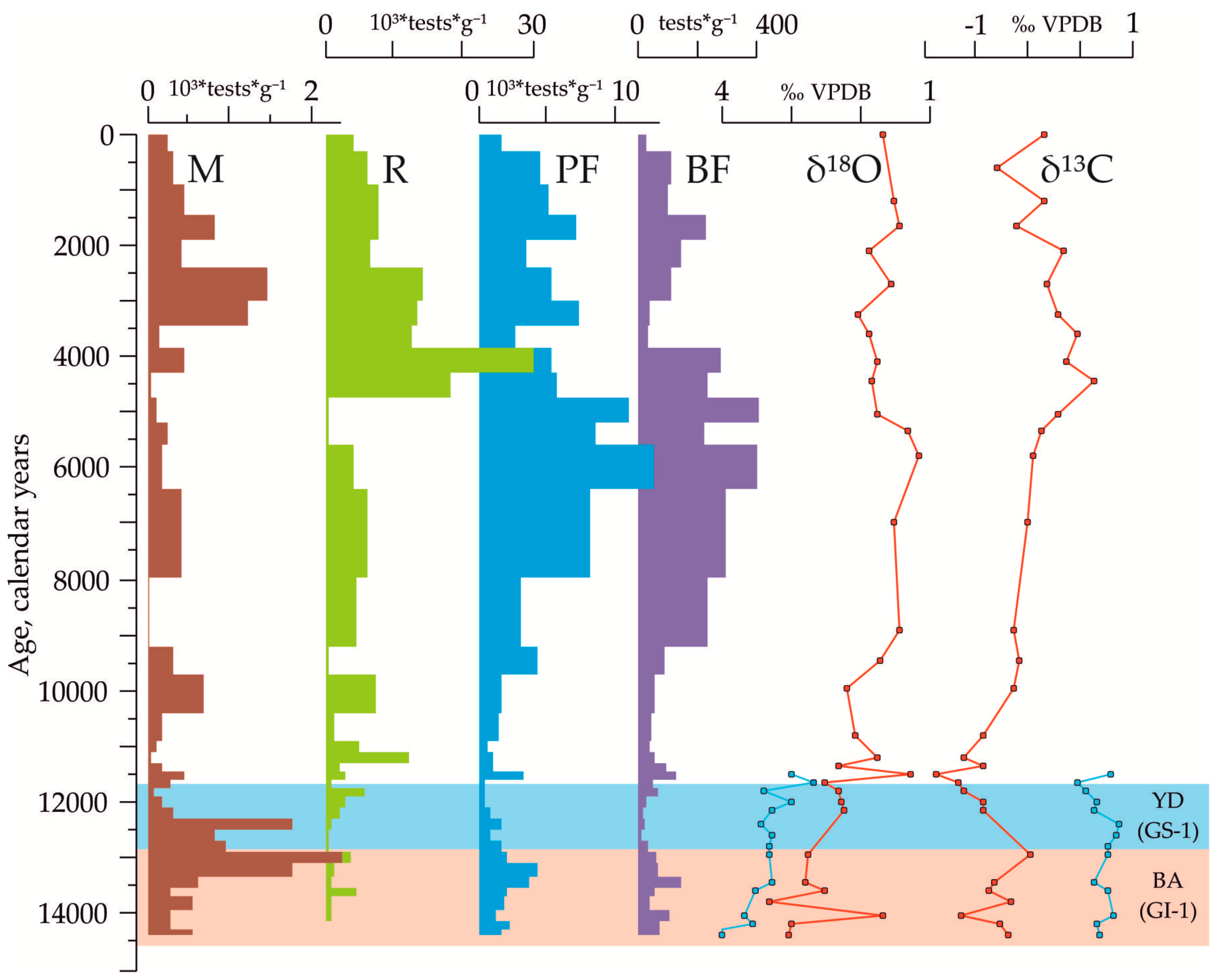
3.2. Indications of the Warm and Cold-Water Events in the Down-Core Records Covering Termination I

The most prominent warming event within the Termination I (BA), and the following cold YD event as a return to the quasi-glacial state had a weak reflection in the records of the total microfaunal abundances (Figure 4). Associated changes in the accumulation of radiolarians and planktic/benthic foraminifera were subtle, with small peaks during the BA and stable low values during the YD.
The response of the main species characterizing the microfossil factors to the paleoclimatic changes within the BA and YD was different (Figure 5). The boreal radiolarian indicator L. spiralis/minor group had high abundances comparable to the modern ones during the BA warming, then decreased in numbers during the cold YD before reaching its typical percentages at the beginning of the Holocene (Figure 5a). Possible increase of the organic matter fluxes to the bottom during the warmings of the BA and at the Holocene beginning can be indicated in the distribution of the benthic foraminifera C. teretis, which feed on the bacteria from the soft, enriched by the organic matter sediments [19]. In contrast, the polar species N. pachyderma (sin.) permanently dominated (40 to 100%) the planktic foraminiferal assemblages both during the warm BA and cold YD, indicating the persistent cold-water conditions on the subsurface depths. The radiolarian species A. setosa, which is typical for cold-water Greenland and Iceland Seas [35], had a prominent peak just in the final part of the BA and earlier part of the YD ca. 13.2–12.3 ka up to 40%, being rare or absent before and after.
We may suppose that a peculiar oceanographic situation existed on the Reykjanes Ridge during this 1-ky time, as high percentages of A. setosa in the Nordic Seas mark environments of the active mixing of cold (down to ca. −2 °C), relatively refreshed Arctic/Polar waters and warmer saline North Atlantic water [37]. Together with A. setosa, a significant increase in the abundances of the mineral grains in the sediment fraction of >100 μm also marks the interval of the YD (Figure 4). Probably, this can be an indication of the Heinrich-like event H-0 as a massive accumulation of the ice-rafted sediment material on the bottom of the northwestern Atlantic Ocean that occurred during the YD [38]. Andrews [39] proposed the Hudson Bay as a source area for the ice-rafted sediments. However, high abundances of the Greenland cold-water radiolarian species A. setosa, which is rare now in the Labrador Sea, could point to the southern Nordic Seas as being the main place of origin place for ice-rafting within the YD on the Reykjanes Ridge.
The final transition toward the recent interglacial state occurred coincidently in all micropaleontological records of the core AMK-340 at the end of the YD. But the first changes indicating the warming started in the middle YD chronozone just after time level of 12.5 ka (Figure 5c,g). For example, the indicator of the open North Atlantic waters, planktic foraminiferal species N. pachyderma (dex.), and benthic foraminiferal species G. subglobosa as a marker of high phytodetrital fluxes [20] significantly increased percentages or even appeared (in the latter case) from this level. Thus, according to our data on the distribution of the microfossils, the final half of the YD might be an interval of the progressed warming on the Reykjanes Ridge at the latitude of ca. 60° N.

3.3. The Stable Oxygen and Carbon Isotope Records in the Core AMK-340

The oxygen isotopic signal δ18O in the planktic foraminiferal shells of both N. pachyderma (sin.) and G. bulloides exhibits a rather monotonous shift (with short deviations but without “heavier” peak during the YD) to the “lighter” values from 14.5 to ca. 11 ka (Figure 4). Alley and Clark [40] summarized the oxygen isotopic data in the planktic foraminiferal shells from the last deglacial sediments in the North Atlantic and noted a significant geographic and temporal variability of the δ18O signal. They also documented the change to the “lighter” δ18O at the BA onset, but no substantial variations during the rest of the deglaciation for the Nordic Seas and open northeastern and northern central North Atlantic. This can be connected with a gradual sea surface warming and salinity increase in these areas. However, the sediment cores at the North America (Nova Scotia) clearly reflected the “heavier” δ18O values during the YD as a result of the melt-water pulses from the deglacial Agassiz Lake [41]. Time interval of 8 to 5.5 ka with lower δ18O values of 1.5–1‰ (Figure 4) can represent a thermal optimum of the middle Holocene within the Atlantic chronozone [42]. This is supported by the prominent peak of the elevated total abundances of the planktic and benthic foraminifera. We are aware that the δ18O changes cannot act as a conclusive paleotemperature index because δ18O of the foraminiferal shells reflect the δ18O of sea water as well governed predominantly by ice volume change on land [43]. Nevertheless, both the temperature increase and lesser ice-volume will lower the δ18O values, which we observe during 8–5.5 ka. Interpretation of the δ13C signal in the planktic foraminiferal shells is more complicated. It is under the influence of the photosynthesis vs. respiration ratio in the surface to subsurface waters, δ13C of the dissolved inorganic carbon, carbonate system parameters, and also temperature [43,44]. Therefore, it is advisable to use δ13C variability in combination with other proxies. In our study, δ13C of G. bulloides had two intervals of the increased values, during the BA and from the early Holocene to mid-Holocene (Figure 4). Rise in the total abundances of radiolarians, planktic and benthic foraminifera also occurred in the same intervals (Figure 4). During the BA, warming and associated possible increase of the organic matter production is evident in the higher δ13C values and percentages of the benthic foraminifera C. teretis, which inhabit surface sediments rich in bacteria and organic matter (Figure 5e). During the Holocene, we recognize an increase in the abundance of benthic foraminiferal species G. subglobosa—marker of spring phytodetrital fluxes, together with the above-mentioned species C. teretis. Thus, we infer that the δ13C values of planktic foraminifera G. bulloides can reflect the increased photosynthetic activity during the warm periods. This is supported, e.g., by studies of the planktic foraminiferal δ13C signal in the last glacial to the Holocene history of the Moroccan upwelling [45].

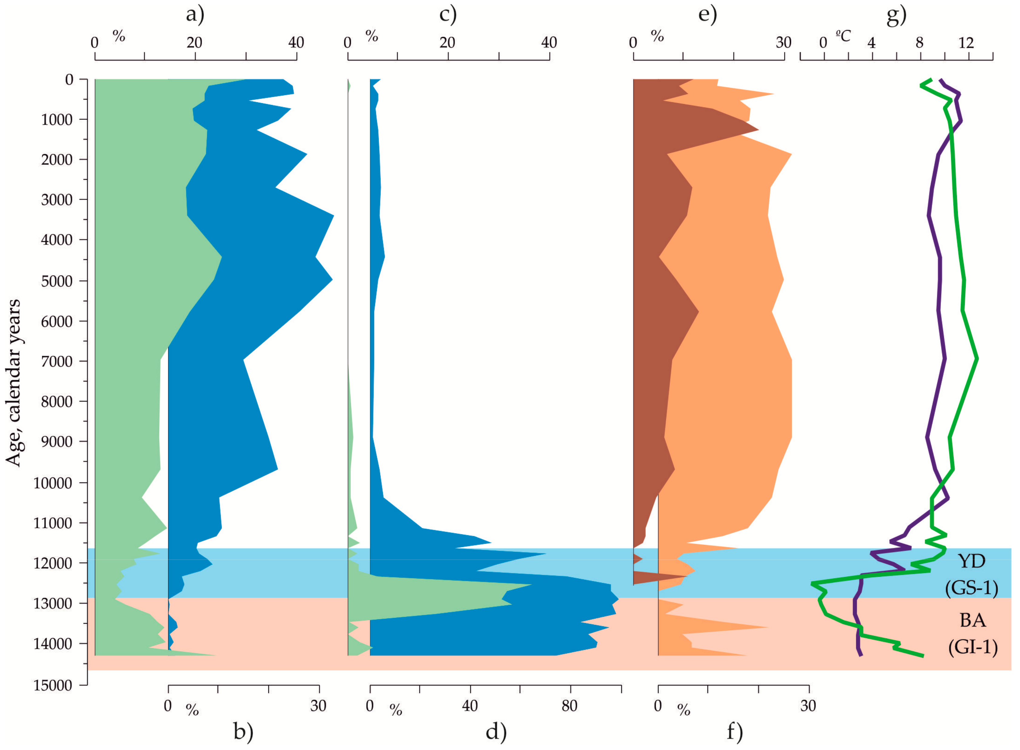
3.4. Paleotemperature Estimates for the Core AMK-340 and Correlation with Other Paleoclimatic Archives

As discussed in the previous subsection, the response of the radiolarian and foraminiferal species from the core AMK-340 on the paleoceanographic oscillations during Termination I was not concurrent. Our micropaleontological records do not coincide in details with the conventional warmings and coolings, the Greenland Stadials and Interstadials [17], at the transition to the Holocene. Reconstructions of the paleotemperature for 100-m water depth (Figure 6b) are also not fully coherent with standard oxygen isotopic archives of the Greenland ice cores [46].
The foraminiferal temperature had monotonous, low values of 2–3 °C from 14.5 to ca. 12.2 ka, and then it started to increase, with some fluctuations, up to 8–10 °C at the beginning of Holocene. Low but weakly variable foraminiferal temperature could arise from the stable dominance of the polar species N. pachyderma (sin.). The monospecific (N. pachyderma (sin.)) planktic foraminiferal assemblages now are distributed in the cold-water Labrador and Nordic Seas within the wide range of summer sea-surface temperatures of 6 to −2 °C [48] or, in our database, summer temperature at 100 m depth of 3 to −1 °C. It could be that the statistical program of the paleotemperature calculations, operating with N. pachyderma (sin.) dominance, may provide less detailed values.
The radiolarian paleotemperature at the BA onset, in contrast, exhibits high values of about 8 °C being comparable with modern and Holocene values in the area. It dropped steadily toward the BA end, and was very low 0 to −2 °C from ca. 13.5 to 12.5 ka, i.e., just until the middle YD cold interval.
The next warming step after the BA, as documented both by the radiolarian and foraminiferal temperatures, occurred in the area of core AMK-340 12.5–12.2 ka (Figure 6c) or considerably earlier than the Holocene started. Neither oxygen isotopic records nor sea-surface paleotemperature estimates on Mg/Ca in the planktic foraminifera, and percentages of the polar N. pachyderma (sin.) from the North Atlantic cores south of Iceland [13,14] (Figure 6a,c) captured such an event. But some other studies support our results. Pearce et al. [49] found the start of the pre-Holocene warming at the time level of 12.2 ka based on the diatom study of the sediment core south of Newfoundland. They concluded the evident difference of the early to late YD local paleoceanography. Ebbesen and Hald [50] reported similar results on the cold YD before 12.5 ka and warmer conditions after this level in the Norwegian Sea. We may see a good visual correlation of this warming step with a sharp change from lower to higher δD values in the Antarctic EPICA ice-core records (Figure 6d) [47]. This can allow us to assume in our records of the subsurface paleotemperature, some correlation to the paleoclimatic changes in the Southern Hemisphere, which was proposed, e.g., by Rickaby and Elderfield [51] for the cooling during the pre-BA Heinrich-1 event and YD, and by Barker et al. [52] for the abrupt paleoclimatic events during the last deglaciation.

4. Conclusions

The North Atlantic areas of the radiolarian and planktic foraminiferal assemblages or main Factors, as defined by the Q-mode analysis of the PanTool Box software, match in their general outlines and reflect a regional biogeography, distribution and interaction of the major cold- and warm-water masses. However, there is a dissimilarity possibly arising from the specific habitat of different radiolarian and foraminiferal species.
The response of the main microfossil species to the paleoceanographic changes within the transition from the BA warming through the cold YD to the warm Holocene was different. The BA warming was well reflected in the radiolarian and benthic but not in the planktic foraminiferal record. The cold-water radiolarian species A. setosa as the Greenland Sea indicator marks cooling at the end of the BA and within the start of the YD event 13.2–12.3 ka. Our micropaleontological and isotopic data along with the paleotemperature estimates for the Reykjanes Ridge at ca. 60° N may document that, after the warm BA, the middle YD ca. 12.5–12.2 ka could be the next significant step toward the Holocene warming in the area of study. It is likely that the paleoceanographic changes in the area of study during the global warming within the Termination I occurred on the subsurface depths earlier than on the sea surface, but future studies are needed to prove this.

Author Contributions

Conceptualization, A.M.; Methodology, A.M., M.S.B., M.T.; Investigation, A.M., M.S.B., T.A.K., P.B., M.T.; Writing—Original Draft Preparation, A.M., M.T.; Writing—Review and Editing, A.M., M.T.

Funding

This research was funded by the Russian Science Foundation and Department of Science and Technology of the Ministry of Science and Technology of India, Joint Project No. 16-47-02009. The funds for the same were extended by National Centre for Antarctic and Ocean Research (NCAOR), Goa, Ministry of Earth Sciences. Funding of the work on the initial micropaleontological data was from the Russian Agency of the Scientific Organization, Project № 0149-2018-0016 for the Shirshov Institute of Oceanology, Moscow, Russia.

Acknowledgments

The authors thank three anonymous reviewers for the constructive criticism and valuable suggestions which helped us to improve the manuscript. The authors are grateful for support from the Russian Government, the Russian Science Foundation, the Russian Agency of the Scientific Organization and the Administration of Shirshov Institute of Oceanology. M.T. and P.B. would like to thank the Secretary, Ministry of Earth Sciences, Govt. of India and the Director, National Centre for Antarctic and Ocean Research for extending support to this project (NCAOR Contribution No. 50/2018). The authors thank R.F. Spielhagen, GEOMAR Helmholtz Centre for Ocean Research, Kiel, Germany, and H. Erlenkeuser, The Leibniz Laboratory for Radiometric Dating and Stable Isotope Research, Christian-Albrechts-University of Kiel, Germany, for providing of the 14C-datings.

Conflicts of Interest

The authors declare no conflict of interest. The founding sponsors had no role in the design of the study; in the collection, analyses, or interpretation of data; in the writing of the manuscript, and in the decision to publish the results.

References

  1. Delworth, T.L.; Zeng, F. The impact of the North Atlantic oscillation on climate through its influence on the Atlantic meridional overturning circulation. J. Clim. 2016, 29, 941–962. [Google Scholar] [CrossRef]
  2. Löfverström, M.; Lora, J.M. Abrupt regime shifts in the North Atlantic atmospheric circulation over the last deglaciation. Geophys. Res. Lett. 2017, 44, 8047–8055. [Google Scholar] [CrossRef]
  3. Knorr, G.; Lohmann, G. Rapid transitions in the Atlantic thermohaline circulation triggered by global warming and meltwater during the last deglaciation. Geochem. Geophys. Geosyst. 2007, 8, Q12006. [Google Scholar] [CrossRef]
  4. Overpeck, J.T.; Peterson, L.C.; Kipp, N.; Rind, D. Climate change in the circum-North Atlantic region during the last deglaciation. Nature 1989, 338, 553–557. [Google Scholar] [CrossRef]
  5. Bauch, H.A.; Kandiano, E.S.; Helmke, J.P. Contrasting ocean changes between the subpolar and polar North Atlantic during the past 135 ka. Geophys. Res. Lett. 2012, 39, L11604. [Google Scholar] [CrossRef]
  6. Matul, A.G. On the problem of paleoceanological evolution of the Reykjanes Ridge region (North Atlantic) during the last deglaciation based on a study of radiolaria. Oceanology 1995, 34, 806–814. [Google Scholar]
  7. Matul, A.G.; Yushina, I.G. Radiolarians in North Atlantic sediments. Ber. Polarforsch. 1999, 306, 35–45. [Google Scholar]
  8. Sieger, R.; Grobe, H. PanTool—A Swiss Army Knife for Data Conversion and Recalculation. Available online: https://doi.org/10.1594/PANGAEA.787549 (accessed on 31 July 2018).
  9. Krauss, W. Currents and mixing in the Irminger Sea and in the Iceland Basin. J. Geophys. Res. 1995, 100, 10851–10871. [Google Scholar] [CrossRef]
  10. Våge, K.; Pickart, R.S.; Sarafanov, A.; Knutsen, Ø.; Mercier, H.; Lherminier, P.; van Aken, H.M.; Meincke, J.; Quadfasel, D.; Bacon, S. The Irminger Gyre: Circulation, convection, and interannual variability. Deep-Sea Res. Part I 2011, 58, 590–614. [Google Scholar] [CrossRef]
  11. Locarnini, R.A.; Mishonov, A.V.; Antonov, J.I.; Boyer, T.P.; Garcia, H.E.; Baranova, O.K.; Zweng, M.M.; Paver, C.R.; Reagan, J.R.; Johnson, D.R.; et al. World Ocean Atlas 2013. NOAA, U.S. Department of Commerce: Washington, DC, USA, 2013; NOAA Atlas NESDIS 73, Volume 1: Temperature. Available online: https://www.nodc.noaa.gov/OC5/woa13 (accessed on 31 July 2018).
  12. Weinelt, M.; Vogelsang, E.; Kucera, M.; Pflaumann, U.; Sarnthein, M.; Voelker, A.; Erlenkeuser, H.; Malmgren, B.A. Variability of North Atlantic heat transfer during MIS 2. Paleoceanography 2003, 18, 1071. [Google Scholar] [CrossRef]
  13. Thornalley, D.J.R.; McCave, I.N.; Elderfield, H. Freshwater input and abrupt deglacial climate change in the North Atlantic. Paleoceanography 2010, 25, PA1201. [Google Scholar] [CrossRef]
  14. Thornalley, D.J.R.; Elderfield, H.; Mc Cave, I.N. Reconstructing North Atlantic deglacial surface hydrography and its link to the Atlantic overturning circulation. Global Planet. Chang. 2011, 79, 163–175. [Google Scholar] [CrossRef] [Green Version]
  15. Zweng, M.M.; Reagan, J.R.; Antonov, J.I.; Locarnini, R.A.; Mishonov, A.V.; Boyer, T.P.; Garcia, H.E.; Baranova, O.K.; Johnson, D.R.; Seidov, D.; et al. World Ocean Atlas 2013. NOAA, Department of Commerce: Washington, DC, USA, 2013; NOAA Atlas NESDIS 74, Volume 2: Salinity. Available online: https://www.nodc.noaa.gov/OC5/woa13 (accessed on 31 July 2018).
  16. Stuiver, M.; Reimer, P.J.; Reimer, R.W. CALIB 7.1 [WWW program], 2018. Available online: http://calib.org (accessed on 31 July 2018).
  17. Rasmussen, S.O.; Bigler, M.; Blockley, S.P.; Blunier, T.; Buchardt, S.L.; Clausen, H.B.; Cvijanovic, I.; Dahl-Jensen, D.; Johnsen, S.J.; Fischer, H.; et al. A stratigraphic framework for abrupt climatic changes during the Last Glacial period based on three synchronized Greenland ice-core records: Refining and extending the INTIMATE event stratigraphy. Quat. Sci. Rev. 2014, 106, 14–28. [Google Scholar] [CrossRef] [Green Version]
  18. Khusid, T.A.; Matul, A.; Barash, M.S.; Gablina, I.F. Benthic foraminiferal records of the last deglaciation on the Reykjanes Ridge. J. Ocean. Res. 2018. submitted for publication. [Google Scholar]
  19. Gooday, A.J.; Lambshead, P.J.D. Influence of seasonally deposited phytodetritus on benthic foraminiferal populations in the bathyal northeast Atlantic: The species response. Mar. Ecol. Prog. Ser. 1989, 58, 53–67. [Google Scholar] [CrossRef]
  20. Suhr, S.B.; Pond, D.; Gooday, A.J.; Smith, C.R. Selective feeding by benthic foraminifera on phytodetritus on the western Antarctic Peninsula shelf: Evidence from fatty acid biomarker analysis. Mar. Ecol. Prog. Ser. 2003, 262, 153–162. [Google Scholar] [CrossRef]
  21. Matul, A.; Mohan, R. Distribution of polycystine radiolarians in bottom surface sediments and its relation to summer sea temperature in the high-latitude North Atlantic. Front. Mar. Sci. 2017, 4, 330. [Google Scholar] [CrossRef]
  22. Index of /Pub/Data/Paleo/Paleocean/Fossil_Plankton/Russian_Fossil_Plankton. Available online: https://www1.ncdc.noaa.gov/pub/data/paleo/paleocean/fossil_plankton/russian_fossil_plankton (accessed on 31 July 2018).
  23. Pflaumann, U.; Duprat, J.M.; Pujol, C.; Labeyrie, L.D. Distribution of Planktic Foraminifera in Surface Sediments of the Atlantic Ocean. 1996. Available online: https://doi.org/10.1594/PANGAEA.51621 (accessed on 31 July 2018).
  24. Zas’ko, D.N. Quantitative distribution of radiolarians in the North Atlantic plankton. Oceanology 2001, 41, 86–93. [Google Scholar]
  25. Rebotim, A.; Voelker, A.H.L.; Jonkers, L.; Waniek, J.J.; Meggers, H.; Schiebel, R.; Fraile, I.; Schulz, M.; Kucera, M. Factors controlling the depth habitat of planktonic foraminifera in the subtropical eastern North Atlantic. Biogeosciences 2017, 14, 827–859. [Google Scholar] [CrossRef]
  26. Colebrook, J.M. Continuous plankton records: Seasonal variations in the distribution and abundance of plankton in the North Atlantic Ocean and the North Sea. J. Plankton Res. 1982, 4, 435–462. [Google Scholar] [CrossRef]
  27. Parsons, T.R.; Takahashi, M.; Hargrave, B. Biological Oceanographic Processes, 3rd ed.; Pergamon Press: Oxford, UK, 1984. [Google Scholar]
  28. Zielinski, U.; Gersonde, R.; Sieger, R.; Fütterer, D.K. Quaternary surface water temperature estimations: Calibration of a diatom transfer function for the Southern Ocean. Paleoceanography 1998, 13, 365–383. [Google Scholar] [CrossRef] [Green Version]
  29. Zielinski, U. Quantitative estimation of palaeoenvironment the Antarctic surface water in the late transfer functions with diatoms. Ber. Polarforsch. 1993, 126, 1–148. [Google Scholar]
  30. Imbrie, J.; Kipp, N.G. A new micropaleontological method for paleoclimatology: Application to a Late Pleistocene Caribbean core. In The Late Cenozoic Glacial Ages; Turekian, K.K., Ed.; Yale University Press: New Haven, CT, USA, 1971; pp. 71–181. [Google Scholar]
  31. Costello, M.J.; Tsai, P.; Wong, P.S.; Cheung, A.K.L.; Basher, Z.; Chaudhary, C. Marine biogeographic realms and species endemicity. Nat. Commun. 2017, 8, 1057. [Google Scholar] [CrossRef] [PubMed] [Green Version]
  32. Boltovskoy, D.; Correa, N. Biogeography of Radiolaria Polycystina (Protista) in the World Ocean. Prog. Oceanogr. 2016, 149, 82–105. [Google Scholar] [CrossRef]
  33. Boltovskoy, D. Foraminifers (Planktonic). In Encyclopedia of Marine Geosciences; Harff, J., Mesched, M., Petersen, S., Thiede, J., Eds.; Springer Science+Business Media: Dordrecht, The Netherlands, 2014; pp. 1–9. [Google Scholar]
  34. Kipp, N.G. New transfer function for estimating past sea-surface conditions from sea-bed distribution of planktonic foraminiferal assemblages in the North Atlantic. Mem. Geol. Soc. Am. 1976, 145, 9–42. [Google Scholar]
  35. Bjørklund, K.R.; Cortese, G.; Swanberg, N.R.; Schrader, H.J. Radiolarian faunal provinces in surface sediments of the Greenland, Iceland and Norwegian (GIN) Seas. Mar. Micropaleontol. 1998, 35, 105–140. [Google Scholar] [CrossRef] [Green Version]
  36. Clark, P.U.; Shakun, J.D.; Baker, P.A.; Bartlein, P.J.; Brewer, S.; Brook, E.; Carlson, A.E.; Cheng, H.; Kaufman, D.S.; Liu, Z.; et al. Global climate evolution during the last deglaciation. Proc. Natl. Acad. Sci. USA 2012, 109, E1134–E1142. [Google Scholar] [CrossRef] [PubMed] [Green Version]
  37. Bjørklund, K.R.; Hatakeda, K.; Kruglikova, S.B.; Matul, A.G. Amphimelissa setosa (Cleve) (Polycystina, Nassellaria)—A stratigraphic and paleoecological marker of migrating polar environments in the northern hemisphere during the Quaternary. Stratigraphy 2015, 12, 23–37. [Google Scholar]
  38. Hillaire-Marcel, C.; de Vernal, A. 2008. Stable isotope clue to episodic sea ice formation in the glacial North Atlantic. Earth Planet. Sci. Let. 2008, 268, 143–150. [Google Scholar] [CrossRef]
  39. Andrews, J.; Jennings, A.E.; Kerwin, M.; Kirby, M.; Manley, W.; Miller, G.H.; Bond, G.; Mac Lean, B. A Heinrich-like event, H-0 (DC-0): Source(s) for detrital carbonate in the North Atlantic during the Younger Dryas Chronozone. Paleoceanography 1995, 10, 943–952. [Google Scholar] [CrossRef]
  40. Alley, R.B.; Clark, P. The deglaciation of the northern hemisphere: A global perspective. Ann. Rev. Earth Planet. Sci. 1999, 27, 149–182. [Google Scholar] [CrossRef]
  41. Keigwin, L.D.; Jones, G.A. The marine record of deglaciation from the continental margin off Nova Scotia. Paleoceanography 1995, 10, 973–985. [Google Scholar] [CrossRef]
  42. Jansen, E.; Andersson, C.; Moros, M.; Nisancioglu, K.H.; Nyland, B.F.; Telford, R.J. The Early to Mid-Holocene thermal optimum in the North Atlantic. In Natural Climate Variability and Global Warming: A Holocene Perspective; Battarbee, R.W., Binney, H.A., Eds.; Wiley-Blackwell: Chichester, UK, 2008; pp. 123–137. [Google Scholar]
  43. Ravelo, A.C.; Hillaire-Marcel, C. The use of oxygen and carbon isotopes of foraminifera in paleoceanography. In Developments in Marine Geology; Hillaire-Marcel, C., de Vernal, A., Eds.; Elsevier: Amsterdam, The Netherlands, 2007; Volume 1, pp. 735–764. [Google Scholar]
  44. Jonkers, L.; van Heuven, S.; Zahn, R.; Peeters, F.J.C. Seasonal patterns of shell flux, δ18O and δ13C of small and large N. pachyderma (s) and G. bulloides in the subpolar North Atlantic. Paleoceanography 2013, 28, 164–174. [Google Scholar] [CrossRef]
  45. Frihmat, Y.E.; Hebbeln, D.; EL Jaaidi, B.; Mhammdi, N. Reconstruction of productivity signal and deep-water conditions in Moroccan Atlantic margin (~35° N) from the last glacial to the Holocene. SpringerPlus 2015, 4, 69. [Google Scholar] [CrossRef] [PubMed]
  46. NGRIP Members. High-resolution record of Northern Hemisphere climate extending into the last interglacial period. Nature 2004, 431, 147–151. [Google Scholar] [CrossRef] [PubMed] [Green Version]
  47. EPICA Community Members. Eight glacial cycles from an Antarctic ice core. Nature 2004, 429, 623–628. [Google Scholar] [CrossRef] [PubMed] [Green Version]
  48. Eynaud, F. Planktonic foraminifera in the Arctic: Potentials and issues regarding modern and Quaternary populations. IOP Conf. Ser. Earth Environ. Sci. 2011, 14, 1–12. [Google Scholar] [CrossRef]
  49. Pearce, C.; Seidenkrantz, M.-S.; Kuijpers, A.; Masser, G.; Reynisson, N.F.; Kristiansen, S.M. Ocean lead at the termination of the Younger Dryas cold spell. Nat. Commun. 2013, 4, 1664. [Google Scholar] [CrossRef] [PubMed] [Green Version]
  50. Ebbesen, H.; Hald, M. Unstable Younger Dryas climate in the northeast North Atlantic. Geology 2004, 32, 673–676. [Google Scholar] [CrossRef]
  51. Rickaby, R.E.M.; Elderfield, H. Evidence from the high-latitude North Atlantic for variations in Antarctic Intermediate water flow during the last deglaciation. Geochem. Geophys. Geosyst. 2005, 6, Q05001. [Google Scholar] [CrossRef]
  52. Barker, S.; Diz, P.; Vautravers, M.J.; Pike, J.; Knorr, G.; Hall, I.R.; Broecker, W.S. Interhemispheric Atlantic seesaw response during the last deglaciation. Nature 2009, 457, 1097–1102. [Google Scholar] [CrossRef] [PubMed]
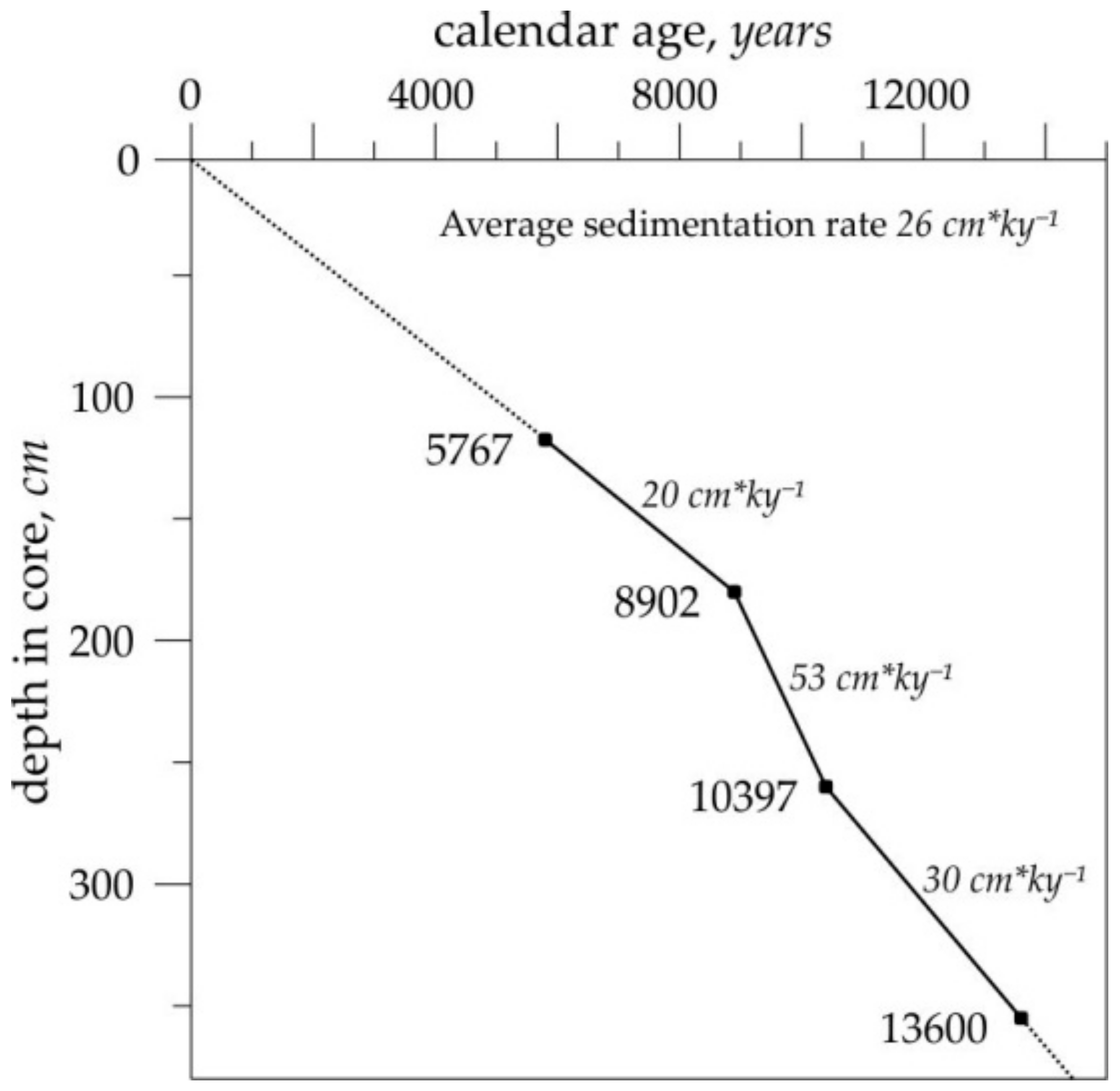
 [Green Version]
Figure 1. Core location (red square) and modern regional oceanography. Sediment cores (yellow squares) were mentioned in the paleoceanographic interpretations: (1) RAPiD-10-1P, (2) RAPiD-12-1K, (3) RAPiD-15-4P [13,14]. Vertical summer salinity and temperature profiles are from the World Ocean Atlas 2013 [11,15]. Red and blue arrows schematically show flows of the warm and cold waters, respectively. GS is Greenland Sea, IP is Iceland Plateau, NS is Norwegian Sea, EGC is East Greenland Current, IC is Irminger Current, SG (IG) is Subpolar (Irminger) Gyre, LS is Labrador Sea, NAC is North Atlantic Current.
Geosciences 08 00375 g001
Figure 2. Age–depth plot for the core AMK-340 based on the AMS (Accelerator Mass Spectrometry) 14C-datings converted to the calendar ages (black squares). Sedimentation rates are displayed. The surface is assumed modern and given a 0 kyr age.
Geosciences 08 00375 g002
Figure 3. Generalized areas of 5 main Factors F1–F5 in the surface sediments of the North Atlantic with for each the loading for planktic foraminiferas (PF) and radiolarians (R), respectively: (a) PF (this study), (b) R (modified from [21] with simplification). F1 loadings >0.6 and >0.8, F2 loadings <−0.9 and >0.9, F3 loadings >0.5, F4 loadings >0.4, F5 loadings >0.1.
Geosciences 08 00375 g003
Figure 4. Main initial micropaleontological, sedimentological and isotopic data on the core AMK-340. M is the number of the mineral grains in the sediment fraction >100 μm calculated per 1 g of dry bulk sediment. R, PF and BF are total abundances of radiolarians, planktic and benthic foraminiferas, respectively, calculated per 1 g of dry bulk sediment. δ18O and δ13C (‰ VPDB) were measured in the shells of the planktic foraminiferas G. bulloides (red line) and N. pachyderma (sin.) (blue line). Light-blue bar is an interval of the cold YD (Greenland Stadial GS-1), rose bar is an interval of the warm BA (Greenland Interstadial GI-1).
Geosciences 08 00375 g004
Figure 5. Down-core distribution of the main radiolarian, planktic and benthic foraminiferal species. Temperate open North Atlantic species: (a) radiolarian L. spiralis/minor group, and (b) planktic foraminifera N. pachyderma (dex.). Subpolar/Polar species: (c) radiolarian A. setosa, and (d) planktic foraminifera N. pachyderma (sin.). Benthic foraminifera: (e) G. subglobosa as marker of spring phytodetrital fluxes [20], and (f) C. teretis as dweller in soft surface sediment, rich on bacterias, being abundant during the summer [19]. Reconstructed temperature for the 100 m water depth, (g): dark-blue line based on the planktic foraminifera, green line based on the radiolarians. Light-blue bar is an interval of the cold YD (Greenland Stadial GS-1), rose bar is an interval of the warm BA (Greenland Interstadial GI-1).
Geosciences 08 00375 g005
Figure 6. Summer paleotemperature for the water depth of 100 m in the core AMK-340 vs other paleoclimatic data: (a) down-core distribution of the polar planktic foraminifera N. pachyderma (sin.) in the cores AMK-340, black line [this study], RAPiD-10-1P, blue line, RAPiD-12-1K, green line, and RAPiD-15-1P, purple line [13,14]; (b) oxygen isotopic curves for the cores AMK-340, dark-green line based on G. bulloides shells and black line based on N. pachyderma (sin.) shells [this study], RAPiD10-1P, blue line based on N. pachyderma (sin.) shells, RAPiD-12-1K, light-green line based on G. bulloides shells, and RAPiD15-1P, purple line based on G. bulloides shells [13,14]; (c) paleotemperature for the cores AMK-340, dark-blue line based on the planktic foraminiferas and dark-green line based on the radiolarians [this study], RAPiD10-1P, blue line based on Mg/Ca in N. pachyderma (sin.) shells, RAPiD-12-1K, light-green line based on Mg/Ca in G. bulloides shells, and RAPiD15-1P, purple line based on Mg/Ca in G. bulloides shells [13,14]; (d) oxygen isotopic curve for the Greenland NGRIP (North Greenland Ice Core Project) ice core, black line [46], and deuterium curve for the Antarctic EPICA (European Project for Ice Coring in Antarctica) ice core [47]. Light-blue bar is an interval of the cold YD (Greenland Stadial GS-1), rose bar is an interval of the warm BA (Greenland Interstadial GI-1), and light-brown bar is a transition to the warmer conditions [this study] within the conventional cold YD.
Geosciences 08 00375 g006
Table 1. List of the accelerator mass spectrometer 14C-datings of the absolute age of the sediment core AMK-340. Conversion of 14C-datings to the calendar ages was made according [16].
Depth in Core14C-Datings, YearsCalendar Age, YearsDating Code
118 cm5480 ± 505767KIA4187
181 cm8030 ± 608902KIA4188
260 cm9220 ± 6010,397KIA4189
356 cm11,830 ± 7013,600KIA4190

