Comparison of Flood Frequency Analysis Methods for Ungauged Catchments in France

Abstract

The objective of flood frequency analysis (FFA) is to associate flood intensity with a probability of exceedance. Many methods are currently employed for this, ranging from statistical distribution fitting to simulation approaches. In many cases the site of interest is actually ungauged, and a regionalisation scheme has to be associated with the FFA method, leading to a multiplication of the number of possible methods available. This paper presents the results of a wide-range comparison of FFA methods from statistical and simulation families associated with different regionalisation schemes based on regression, or spatial or physical proximity. The methods are applied to a set of 1535 French catchments, and a k-fold cross-validation procedure is used to consider the ungauged configuration. The results suggest that FFA from the statistical family largely relies on the regionalisation step, whereas the simulation-based method is more stable regarding regionalisation. This conclusion emphasises the difficulty of the regionalisation process. The results are also contrasted depending on the type of climate: the Mediterranean catchments tend to aggravate the differences between the methods.

1. Introduction

In France, floods by river overflowing are the first natural risk endangering the population, with more than 17 million people exposed [1]. To reduce disaster risk and to effectively protect people, goods and infrastructures, it is essential to correctly assess and map the natural hazard at the origin of any natural disaster. In hydrology, this particular topic is called flood frequency analysis (FFA). It aims to associate flood intensity (generally in terms of discharge) with its probability of exceedance (in terms of return period). This kind of knowledge is essential for diverse operational applications such as flood prevention or civil engineering design (dams, dykes, any construction near a river).

A quite abundant literature [2,3] has been published on developing and comparing different FFA techniques to best estimate extreme flood intensity (T > 100 years) based on the exploitation of a limited number of flow observations (a few years or decades). In this case, the problem can be regarded as a frequency extrapolation issue. On this matter, most studies focus on fitting a probability distribution (commonly a generalised extreme value (GEV) distribution in the case of annual maximum flow sampling) to the sample data [4]. Despite substantial attention paid to the distribution fitting technique [5,6,7,8], the main limitation with this kind of local statistical approach remains the availability and amount of flow data at the site of interest [9]. Indeed, the non-linearity of hydrological processes makes the extrapolation of flood frequency curves problematic [4]. Most particularly, the presence or absence of extreme events within the observation period makes it difficult to assess the distribution skewness. In the case of the GEV distribution, the shape parameter is particularly sensitive to the sampling of flow data. This problem can lead to huge uncertainty over the estimated low-frequency quantiles.

For this reason, alternative approaches have emerged. They are based on enriching the data set with another source of information. On the one hand, pooling data from neighbouring catchments provides a more stable estimation of the distribution parameters. This can be achieved by merging local and regional data [10] or by identifying regional distributions describing the behaviour of all inner catchments [11,12,13]. Regional information can also be used to inform the fitting of at-site distribution [14]. These approaches remain purely statistical. On the other hand, it is possible to use a more process-based approach. In this case, rainfall information is used. This information is easier to determine due to more homogeneous phenomena and better observation. The main idea is to use both the statistical properties of rainfall and information on rainfall-runoff transformation [15,16,17]. In this way the non-linearity of rainfall-runoff transformation can be explicitly taken into account. For instance, a rainfall generator can be coupled to a rainfall-runoff model in order to simulate long flow time-series from which flood quantiles can be extracted [18,19].

As for all hydrological studies on ungauged sites, FFA without at-site data requires a regionalisation step. That is to say, it is necessary to transfer some kind of information from gauged sites where this information is known to the target ungauged site [20]. In FFA, regionalisation can be implemented in two different ways: by directly transferring the flood quantiles [21,22,23] or by transferring the FFA parameters. These parameters could be either statistical distribution parameters [24,25,26] or a rainfall-runoff parameter [27]. Another solution is the application of a regional distribution to an ungauged catchment using the regionalisation of a scaling flow index [13,28,29]. More generally, regionalisation methods intend to estimate an unknown variable by either inferring it from physiographic catchment descriptors [26,30,31] or combining the values from similar catchments [32,33] or neighbouring ones [23,34,35].

The multiplicity of regionalisation methods has led to a number of comparative studies. For instance, comparisons between quantile regionalisation and parameter regionalisation have been proposed on 237 North-Eastern USA catchments [26] and 53 Australian basins [25]. Both studies found slightly better performance for the quantile regression techniques (especially for rare events) but still consider parameter regionalisation as a useful alternative. A wide range of regionalisation techniques were comparatively applied by Merz and Blöschl [36] for distribution parameters over 575 Austrian catchments. This study highlights the good performance of methods based on both the spatial proximity of catchments and their physical characteristics.

At this stage it appears quite obvious that multiple choices have to be made when selecting an FFA method for an ungauged catchment: the FFA method, the variable to regionalise and the regionalisation technique. Indeed, numerous countries have developed their own methodological framework to unify the techniques employed by the different flood risk practitioners. This is the case of the United Kingdom [37,38], Spain [39], the USA [40,41], Australia [42,43] and a number of European countries [2]. Surprisingly, France does not have this kind of framework. Most of the time, operational FFAs are implemented by fitting a statistical distribution to local data in gauged sites or by estimating flood quantiles through empirical relationships called “rational” approaches [44]. Recent studies implemented a data-based comparison of diverse FFA methods used in France [9] and concluded that methods using regional data or exploiting the rainfall information should be preferred to purely at-site statistical data [18,45]. Nevertheless, the transfer of this kind of FFA method to ungauged catchments has remained limited with only one regionalisation method tested and the performance was insufficient to draw general conclusions [45].

The objective of the present paper was to assess the relative performance of different regionalised FFA techniques for application to ungauged catchments. Different FFA methods were applied and associated with diverse regionalisation techniques. The FFA methods were an at-site Gumbel distribution (also called GEV type I), an at-site GEV distribution fitted with a Bayesian process using a regional a priori, a regional GEV distribution fitted on pooled data (the index flood method) and a process-based simulation approach (the SHYREG method [18,46,47]). To be as exhaustive as possible, different regionalisation schemes were associated with each of the FFA approaches. We considered an inverse weighted distance method, a similarity-based linear combination approach and a multiple linear regression inference. These regionalisation methods are very simple and would probably be outperformed by more sophisticated methods (e.g., kriging, non-linear inference), but the wide scope of the present comparison study required simplicity. In addition, these methods cover quite a wide range of regionalisation types (spatial interpolation, physical inference, region of influence). To produce coherent quantiles with different return periods, we chose to focus on parameter regionalisation techniques; nevertheless, a brief quantile regionalisation attempt is also discussed.

This comparison study was processed over a large set of 1535 catchments distributed throughout France. All the approaches tested were compared in a single framework independently of the nature of the methods used [9]. This framework is built on a k-fold cross-validation procedure in order to consider the different catchments in an ungauged configuration.

The following sections first describe the data set used and the different methods employed (FFA and regionalisation). The results of the study are provided in Section 3, whereas discussions and conclusions are drawn in the final two sections.

2. Materials and Methods

2.1. Data

2.1.1. Gauged Basin Information

So that general conclusions could be drawn, it was necessary to use a large and diversified set of catchments. A large number of catchments allows for reliable statistical analysis and splitting sample tests, whereas diversity in catchment types ensures the possibility of generalisation to other catchment sets. For this purpose, it appears suitable to use catchments from all over France because this country is characterised by a dense river monitoring network and diversity in terms of climate, geology and morphology.

Here, we intended to test the ability of different FFA approaches to be transferred to other sites (i.e., regionalised); consequently, it appeared more important to obtain a large data set even with a limited amount of available discharge data. We analysed maximum annual peak flow values extracted from time-series with at least 10 years of observation because peak flow is of greater interest when characterising floods for small catchments. The data were extracted from the HYDRO database [48]. Several quality indices were also extracted or calculated (indices from the database, seasonality, presence of upstream dams, spatial homogeneity, knowledge of the drainage area, replaced station) and the decision to keep or remove a catchment was taken manually on a case-to-case basis when these indices reached certain thresholds values.

Finally, 1535 gauged catchments were selected. Their location is provided on Figure 1. It can be seen on

Table 1. Characteristics of the catchment set.

Characteristics	Min	1st Quartile	Median	3rd Quartile	Max
Observation periods (years)	10	24	37	44	116
Area (km2)	1.5	86	198	599	10010
Annual precipitation (mm)	355	791	895	1055	1862
Median resized peak flood (m3·s−1·km−1.6)	0.73	10.5	17.8	28.3	241

that drainage areas range from 1 to 10,000 km². The catchment size was limited because the largest catchments are often human-impacted, gauged and consequently not within of the scope of this study. It appeared obvious that the drainage area was the first factor explaining the variability of flood magnitude. This size effect was taken into account in the different regionalisation methods by resizing all flow data from all catchments to a virtual catchment of 100 km² as described by Equation (1) (see for example [36]). In this equation, $Q$ is the resized discharge variable, $Q_A$ is the real discharge variable for a catchment of drainage area $A$ (km²) and $\beta$ is a constant set to 0.8. This $\beta$ value was determined by fitting a log-linear model to the frequent flood quantiles against the catchment size relationship for the whole data set. The resized flows are proportional to the specific flows. From here on, only the resized discharge values are used.

$$Q=Q_A{\left(\frac{100}{A}\right)}^{\beta }$$

(1)

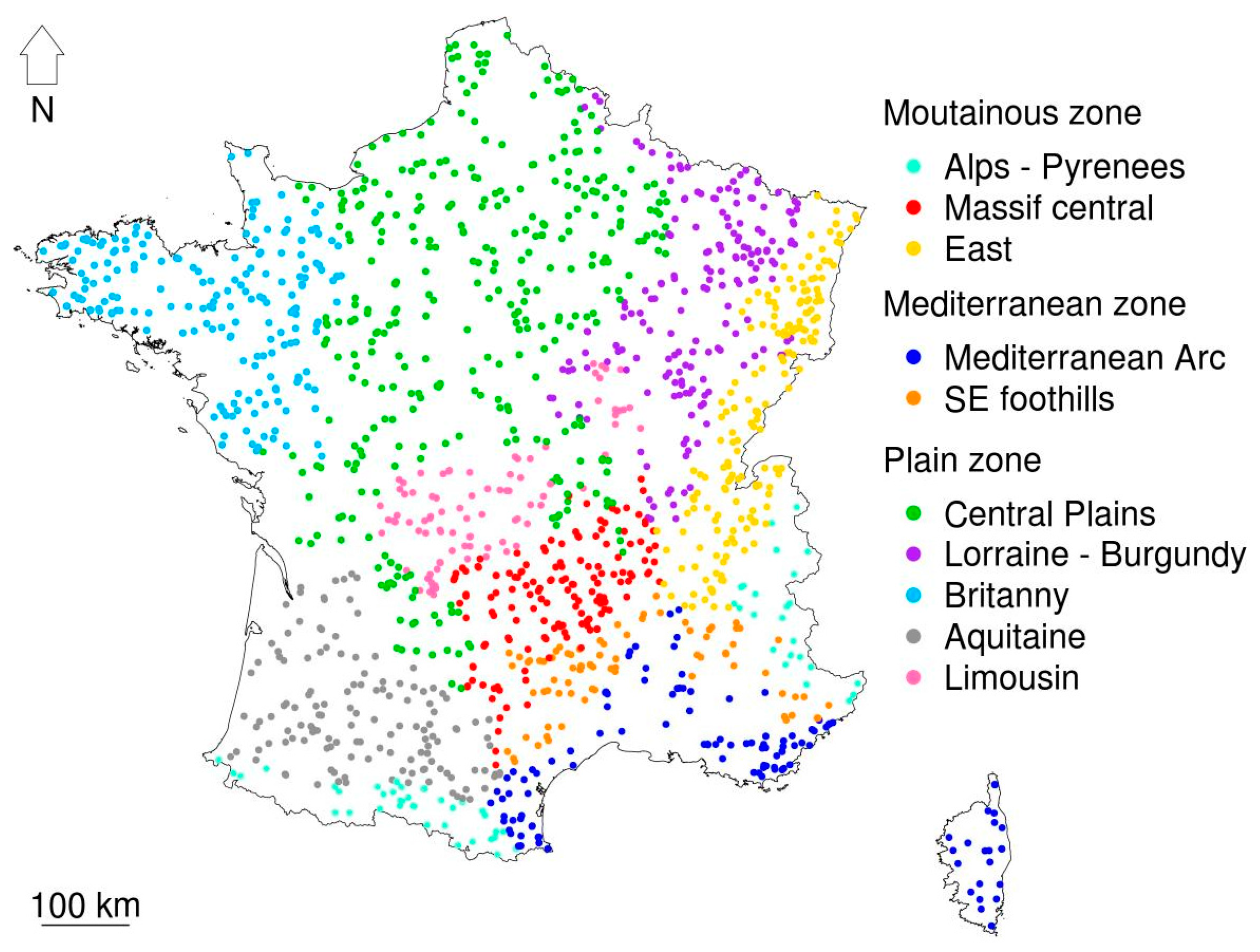
2.1.2. Regional (ised) Information

Different regionalisation techniques are based on catchment descriptors such as environmental variables characterising catchments but not extracted from discharge time-series. Consequently, they are assumed to be (and must be) available over the whole study area. Obviously the number, nature and quality of these descriptors mainly depend on the place where the study is conducted.

The continuous variables were averaged over all catchments and the percentage of presence of the different categorical descriptors was also extracted. For percentage data, an arcsine square root transformation [49] was used for normalization; this transformation is detailed in Equation (2), where x is the raw variable and x* the transformed variable. The different descriptors and their origin are summarised in

Table 2. Catchment descriptors.

Type	Source	Variable	Name
Climate	SAFRAN [50] Budyko formula [51]	Aridity index	Arid
	SAFRAN [50]	Annual mean evapotranspiration	ETP
		Annual mean solid precipitation	Snow
		Annual mean liquid precipitation	Rain
		Annual mean temperature	T
	SAFRAN [50] and Aubert [52]	Annual mean soil moisture	SAJ
		Mean soil moisture prior to a rainy event (>20 mm)	SAJ20
	SHYREG rainfall maps [53]	Mean duration of rainfall events	DT
		Mean number of rainfall events per season	NE
		Mean intensity of rainfall events	PJ
Morphology	From Carthage database [54]	River network density	DDr
Topography	Copernicus [55]	Mean elevation	Alt
		Mean slope	Slope
Hydrogeology	Aubert [52] from Margat [56]	Capacity of the SHYREG production reservoir	AHg
	ESDB [57]	Presence of sand bedding	HGsand
		Presence of rock bedding	HGrock
		Low infiltration capacity class	LOWcapa
		Medium infiltration capacity class	MEDcapa
		High infiltration capacity class	HIGHcapa
Land use	Corine Land Cover [58]	Forest cover	Forest
		Arable cover	Arable
		Grassland cover	Grassland
Catchments	Banque Hydro [48]	Catchment area	Area
		Catchment eastening	X
		Catchment northening	Y
Regions	Hydro-Eco-Regions [59]	Hydro-Eco-Regions	/

.

$$x^{*}=\arcsin \left(\sqrt{x}\right)$$

(2)

To work over more uniform areas, France’s land area was split into several regions, which were constructed a priori according to the existing hydro-eco regions [59]. The definition of French sub-regions according to those hydro-ecoregion is somehow common in hydrology, for example, in flood analysis [10,60], low flows estimation [61]. To retain a sufficient number of gauge stations in each of the regions, the number of regions was limited to ten. To identify the most similar hydro-eco regions, a multiple factor analysis (MFA) was performed over all the descriptor sets where groups were defined according to the descriptor type (see Table 2). Reunifications were performed between neighbouring regions both in space and in the variable graph from the MFA. The resulting split is presented on Figure 1. For the sake of comparability, the same delineation was employed for the regionalisation of the different FFA methods even if the variable at stakes were very different. The choice of a more specific delineation for each variable may be a good perspective to improve each method independently.

For a study area as diverse as France, it was useful to discriminate the results by region. Nevertheless, to limit the number of plots in the article we decided to design three macro-regions by merging some of the ten regions:

• Plains zone: Central Plains, Lorraine-Burgundy, Brittany, Aquitaine, Limousin
• Mountainous zone: Alps-Pyrenees, Massif Central, East
• Mediterranean zone: Mediterranean Arc, South-East foothills.

These three macro-regions were only used for presentation and interpretation of the results.

All raster data have been treated with the raster library [62] from the R software [63]. MFA analysis have been carried out with the FactoMineR library [64].

2.2. FFA Methods

All the procedures implemented associate an FFA approach and a regionalisation scheme. The FFA approaches require calibration against at-site flow data. Then the regionalisation schemes estimate a value of interest at an ungauged catchment by transferring it from gauged catchments. Hereafter, this association is called a regionalised FFA. This part aims to present the different candidates for the first component.

2.2.1. At-Site Statistical Distribution

Fitting a probability distribution against local data is probably the most common form of FFA. It is a direct application of the extreme values theory [65]. Nevertheless, within this FFA family many different implementations exist.

In the present case, we decided to use annual maxima data, fitted with a GEV distribution, which seems to be a common choice for French catchments [9,45]. The cumulative distribution function of the GEV distribution is provided by Equations (3) and (4), where $F\left(x;\mu ,\sigma ,\xi \right)$ is the cumulative distribution function, $\mu$ the location parameter, $\sigma$ the scale parameter and $\xi$ the shape parameter.

$$F\left(x;\mu ,\sigma ,\xi \right)=e^{-t\left(x\right)}$$

(3)

$$t\left(x\right)=\{\begin{array}{l}{\left(1+\left(\frac{x-\mu }{\sigma }\right)\xi \right)}^{-1/\xi }\hspace{1em}\hspace{1em}if \xi \ne 0\\ e^{-\left(x-\mu \right)/\sigma }\hspace{1em}\hspace{1em}\hspace{1em}\hspace{1em}\hspace{1em}\hspace{1em}if \xi =0\end{array}$$

(4)

Since the shape parameter is difficult to estimate with short records and has a great impact on large return period quantiles, we imposed a zero value. This two-free-parameter distribution is called the Gumbel distribution (or GEV type I). This choice appears to be more satisfactory than a three-free-parameter GEV distribution fitted with only at-site data [45]. The distribution was fitted with a Bayesian approach using non-informative flat priors for both parameters. In all cases when a Bayesian procedure was used, a metropolis sampler [66] was employed to determine the posterior distribution of each parameter. The GEV likelihood function is extracted from the evd library [67]. This FFA method is denoted GUMBEL throughout this article.

2.2.2. Local-Regional Statistical Distribution

To observe the impact of the complexity of the distribution, a three-parameter GEV distribution was used (see Equations (3) and (4). To deal with the difficulty estimating the shape parameter, a Bayesian local-regional approach was employed [14,45]. The main objective was to enrich the local information with regional information to constrain the fitting process. In this Bayesian procedure, regional information was used as priors and the local data as observation. The final GEV parameters were derived from the posterior distribution:

• The GEV distribution was fitted at each site using only local data with a Bayesian procedure (with a flat prior for both the location and scale parameters and a normal prior with a 0.25 mean and standard deviation for the shape parameter).
• Each GEV parameter was related to catchment descriptors by a linear regression (independently in each of the ten regions).
• A new GEV distribution was fitted using a Bayesian approach, using informative priors based on the results of the regression. This FFA method is denoted GEV_LR throughout the article.

2.2.3. Regional Distribution

The index flood procedure [13,68] is a regional approach which intends to pool the observations from all catchments in a given region so that a single regional frequency distribution curve (i.e., the growth curve) can be obtained. To handle local and size effects, all data from a gauged catchment must be un-dimensionalised by a local index (the so-called index flood), and the growth curve is a dimensionless probability distribution. The pooling of different sites increases the quantity of data and makes it possible to fit a distribution more reliably [69]. To make predictions on ungauged sites, the index flood needs to be regionalised, a commonly applied procedure [28,29,37,70].

The history of the index flood method in France is quite limited (nonetheless, an example over a limited study area can be found in [10]), contrary to the United Kingdom, for instance, where national guidance has been drawn up [38,71]. The development and design of a more complete, high-performance and presumably complex index flood procedure is not within the scope of this paper. Here the aim was to investigate the relative merits of different FFA and regionalisation approaches. Consequently, we adopted a very simple procedure. First, the national land area was divided into ten regions identical to those presented in Section 2.1.1. By making this choice, we assumed that a physical similarity between catchments is equivalent to a hydrological similarity, which is obviously questionable [72]. Nevertheless, the French hydro-eco regions are commonly used as hydrologically similar regions [10,60]. To ensure independency between the events, only flood events at least 3 days apart were pooled in each region. For each catchment, the index flood was chosen as the mean maximum annual flood. The growth curve was derived by fitting a GEV distribution to the pooled data using the same procedure than for local procedure (see Section 2.2.1). This growth curve is assumed to describe the probability of exceedance of dimensionless floods in the whole region.

At this point, it should be remembered that the size effect had already been removed using resized flows, so the index flow only accounted for local effects. The use of resized flows is generally not necessary for the index flow procedure but was adopted here for the sake of homogeneity with other approaches. The objective of the regionalisation was then to estimate the index flood in the different ungauged catchments.

This method is denoted INDEX FLOOD throughout the article.

2.2.4. Process-Based Method

The application and development of the SHYREG process-based and simulation approach has a long history in France [52,73,74,75]. The quantile estimation is conducted in three stages:

• A fully regionalised at-site stochastic rainfall generator is used to simulate long series of rainfall events at any point in France (kilometric resolution) at an hourly time-step. The development, calibration, regionalisation and validation of this generator have been the object of numerous studies [47,76,77,78] and are not within the scope of this paper. This generator is included in national guidance for rainfall prediction in France [79].
• A conceptual, hourly and event-based rainfall-runoff model with two reservoirs transforms at-site rainfall events into at-site flood events at the kilometric resolution. This model is a simple GR-type model [80,81] with a single parameter to calibrate. It is composed of a production reservoir whose capacity is related to hydrogeology, a routing reservoir with a uniform capacity and a 2-h unit hydrograph [46]. During a rainfall event, the production reservoir retains water and progressively saturates. This progressive saturation of the model simulates a non-linear rainfall-runoff transformation which can be related to the progressive saturation of the catchment. For more extreme events, saturation becomes complete and all the exceeding water participates in runoff. In this case, the runoff is controlled by the rainfall information. The only calibrated parameter of this model is the initial filling of this production reservoir. At-site flood quantiles are extracted directly from the empirical distribution of flood events.
• The at-site flood quantiles are aggregated to catchment outlets using an areal reduction function solely depending on the drainage area and the simulation time-step [46]. The calibration of the model aims to determine which specific flows (associated with a certain value of the parameter) should be aggregated to minimise the error between the 2-, 5- and 10-year return period SHYREG-simulated quantiles and GEV quantiles for flood peaks and daily flows. The optimal value of the parameter is then attributed to the whole catchment.

The SHYREG flood quantiles (in gauged sites) were evaluated in previous studies [18,45], which demonstrated the high stability of the approach regarding calibration data and better accuracy than at-site distribution fitting, especially regarding high return period quantiles.

Another advantage of the SHYREG method is its capacity to simulate multiple time-step quantiles (from peak flow to 3-day flows) with a single calibration parameter. That is why it is calibrated with both daily and peak flows. Consequently, a single regionalisation is needed, whereas other FFA approaches would require a different implementation and regionalisation for each time-step.

2.3. Regionalisation Schemes

This section aims to present the candidate techniques used to transfer FFA to ungauged sites.

To be able to assess the ability of the different approaches to perform in ungauged basins, one must use observed data, which do not exist in these ungauged catchments. Consequently, a part of the catchment set can be considered as falsely ungauged and its data used solely to calculate validation indices. We define two types of catchments:

• Donor catchments: sites where all data were assumed to be available; they could be used to calibrate both the FFA and the regionalisation method.
• Target catchments: sites where the flood quantiles were to be estimated; the discharge data could only be used to perform validation.

The most common donor/target split is probably the leave-one-out cross-validation. In this approach, each gauged catchment is alternatively used as the target and estimation is performed by running the whole procedure using the other basins as donors. This kind of procedure was judged computationally too costly due to the number of methods implemented. In addition, considering the size of the catchment set it is assumed that the removal of a single basin would not affect the design of the regionalisation scheme. To overcome these issues, we adopt a lighter k-fold cross-validation procedure. In this case, 90% of the catchments are used as donors, whereas the remaining 10% are the target sites where validation is performed. The procedure is repeated ten times, so each catchment is used as a target at some point. Consequently, by recombining the quantile estimations, it is possible to obtain a set of quantile estimations for each catchment considered as ungauged.

We also tested more data-scarce configurations by decreasing the percentage of available donors (from 90% to 33%) to evaluate the impact of the river monitoring network density on the performance of the regionalised FFA. In all cases, the samples were randomly selected in each of the ten sub-regions to ensure a smooth spatial distribution of donor and target sites.

One should keep in mind that each catchment was alternatively used as donor and target (in different sampling applications). The same sampling methods were applied for all the regionalised FFAs.

It should be noted that leave-one-out procedures were occasionally employed to calibrate the regionalisation schemes. In this case the only catchments used were the donors, and no validation was involved.

2.3.1. Spatial Proximity

Regionalisation based on spatial proximity assumes that close sites will be more similar than more distant sites. The methods range from the simple inverse distance weighted method to the more complex kriging method [23,34]. In comparative studies, the spatial proximity method demonstrated their good performance over purely physical regionalisation [35,36,82].

Here we adopted a simple inverse distance-weighted procedure. The value of interest at a target site was estimated by linear combination between the neighbouring donor catchments. The distance is measured between the centroids of the catchments. The approach is summed up by Equations (5) and (6), where ${\widehat{\theta }}_i$ is the estimation of the variable of interest at the target site i, ${\theta }_j$ is the known value of the variable of interest at the jth closest donor catchment (among n available donor catchments), $w_{ij}$ is the weight attributed to donor site j for the estimation of that target site, $\alpha$ is a constant and $d_{ij}$ is the Euclidian distance between the centroids of catchments i and j.

$${\widehat{\theta }}_i={\displaystyle \sum }_{j=1}^n{w}_{ij}{\theta }_j$$

(5)

$$w_{ij}=\frac{1/{d_{ij}}^{\alpha }}{{{\displaystyle \sum }}_{k=1}^{n}1/{d_{ik}}^{\alpha }}$$

(6)

In the present case, $\alpha$ was automatically optimised to best reproduce the variable of interest at the donor sites (leave-one-out procedure among the donor catchments) and different values of n, the number of donor catchments to be included in the neighbourhood, were implemented.

This kind of spatial proximity regionalisation can be seen as a sort of region of influence approach [33], where the similarity measure is based only on proximity.

The same method was also used to implement a spatial interpolation of the regression residuals in the regression-based regionalisation presented below.

2.3.2. Similarity Pooling

The second regionalisation method was also a region-of-influence approach [33], but this time the selection of donor catchments was based on a similarity measure. Several similarity metrics have been published in the literature: they are generally defined as an Euclidian distance in a hyperspace defined by various catchment descriptors, the number and types of these descriptors being based on expert judgement or a trial-and-error procedure [82,83,84,85,86]. The regionalisation can also be described by Equations (5) and (6), but this time $n$ is the number of similar catchments in the pool and $d_{ij}$ is the distance between the ith target site and its jth most similar site in the hyperspace.

In the present study, for the sake of reproducibility and generalisation we implemented a procedure of automatic selection of the descriptors. This procedure is intended to select the set of descriptors providing the best estimation (in the sense of the root mean square error) of the value of interest at the donor catchments by means of a leave-one-out procedure among these donors. The same set of descriptors was then used to estimate the same value at the target sites.

This is a stepwise procedure testing the progressive addition or removal of the different descriptors in the similarity metrics. When a metric is tested, the distance matrix between all the donor catchments is calculated (according to the metric) and for each of these basins the n most similar ones are selected. Therefore, given this metric it is possible to estimate the value of interest at each basin and to calculate an error criterion. The addition or removal of a variable from the previously selected metric is decided according to the progression of this error criterion. This procedure is very similar to the stepwise algorithm commonly employed for covariate selection in a linear regression, the main differences being the structure of the model and the leave-one-out context, which is not systematic in the case of linear regressions.

2.3.3. Regression-Based Method

The objective of regression-based regionalisation is to explain the value of the variable of interest with catchment descriptors instead of combining values from selected donor catchments. Many examples of regressions can be found for the regionalisation of flood quantiles [25,26,87], the probability distribution parameter [25,26,36], the hydrological model parameter [30,31,35] or the index flood [70]. Different methods have been developed and proposed to enhance the predictive power of these regressions: variable transformation [87], regression over smaller regions [88], generalised linear models [21], regression over principle components [30], Bayesian models [25] and spatial regression [26].

Here we adopted an ordinary least square linear model as described in Equation (7), where ${\widehat{\theta }}_i$ is the estimated variable of interest at the ith target site, ${\beta }_j$ (j between 0 and p) is the regression parameter to determine, $p$ is the number of covariates used (i.e., catchment descriptors) and $x_{k,i}$ is the value of the kth covariate at the ith target site. The regressions were alternatively fitted on the whole study area and on each of the ten regions described on Figure 1.

The covariates to be included in the model were selected using a common algorithm which progressively tests the benefits of adding or removing a covariate to the model. The selection criterion used is the Akaike Criterion Information [89], whose benefit is to penalise models with too many variables. In all cases, the stepwise algorithm was implemented over the set of donor catchments and then the selected model was applied to the target sites.

To account for some non-linear relationships with the covariates, log-transformations of the variable of interest and/or covariates were also tested.

$${\widehat{\theta }}_i={\beta }_0+ {\displaystyle \sum }_{k=1}^p{\beta }_k{x}_{k,i}$$

(7)

Regression analysis have been implemented with the stats library [63] for the R software.

2.4. Evaluation Criterion

The present analysis focused on the evaluation of flood quantiles in ungauged sites. Consequently, the different evaluations were only performed on quantiles estimated in target sites. We used three criteria:

• The R² criterion evaluated the goodness-of-fit between two estimations in many sites of the same value.
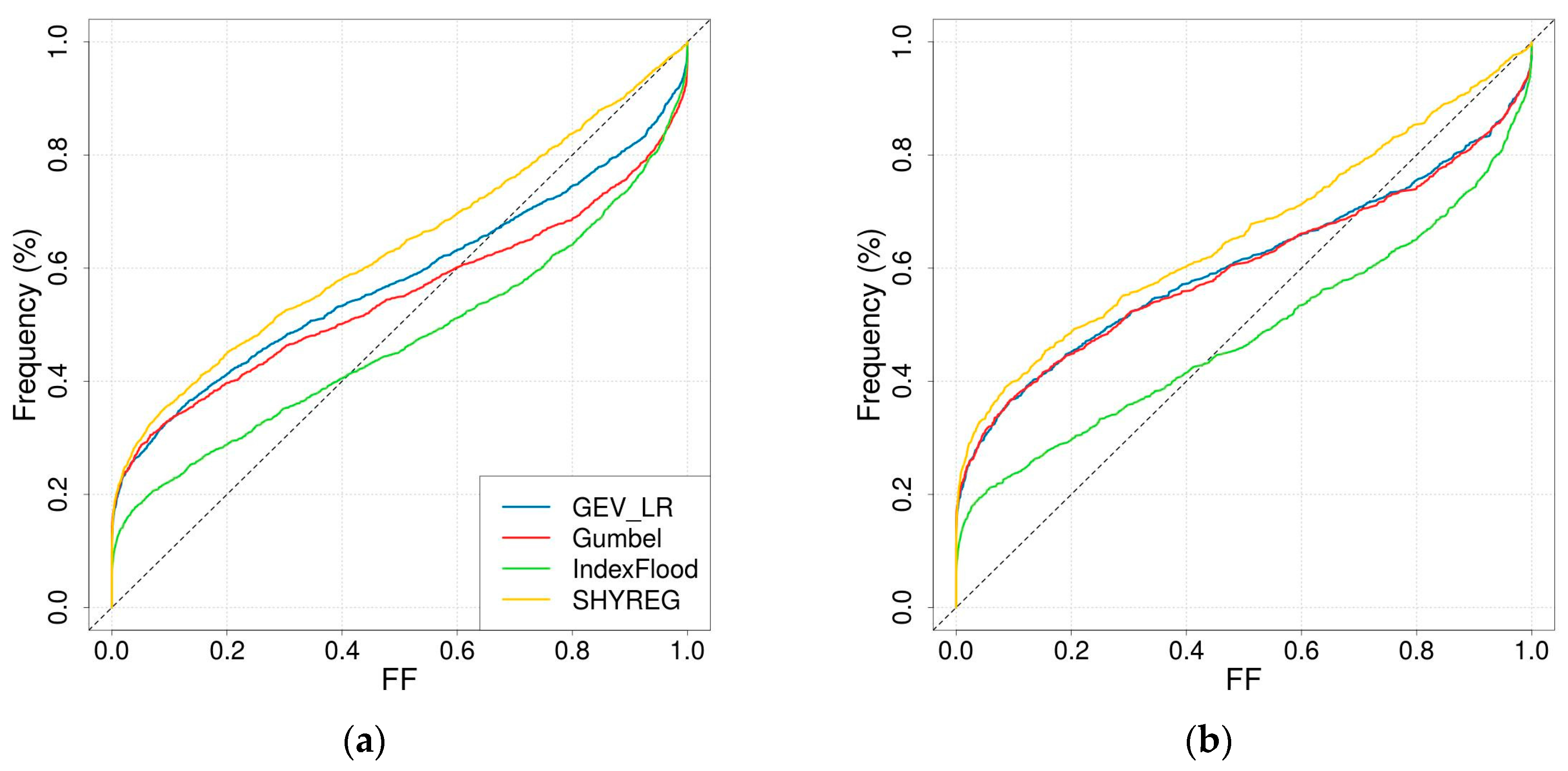
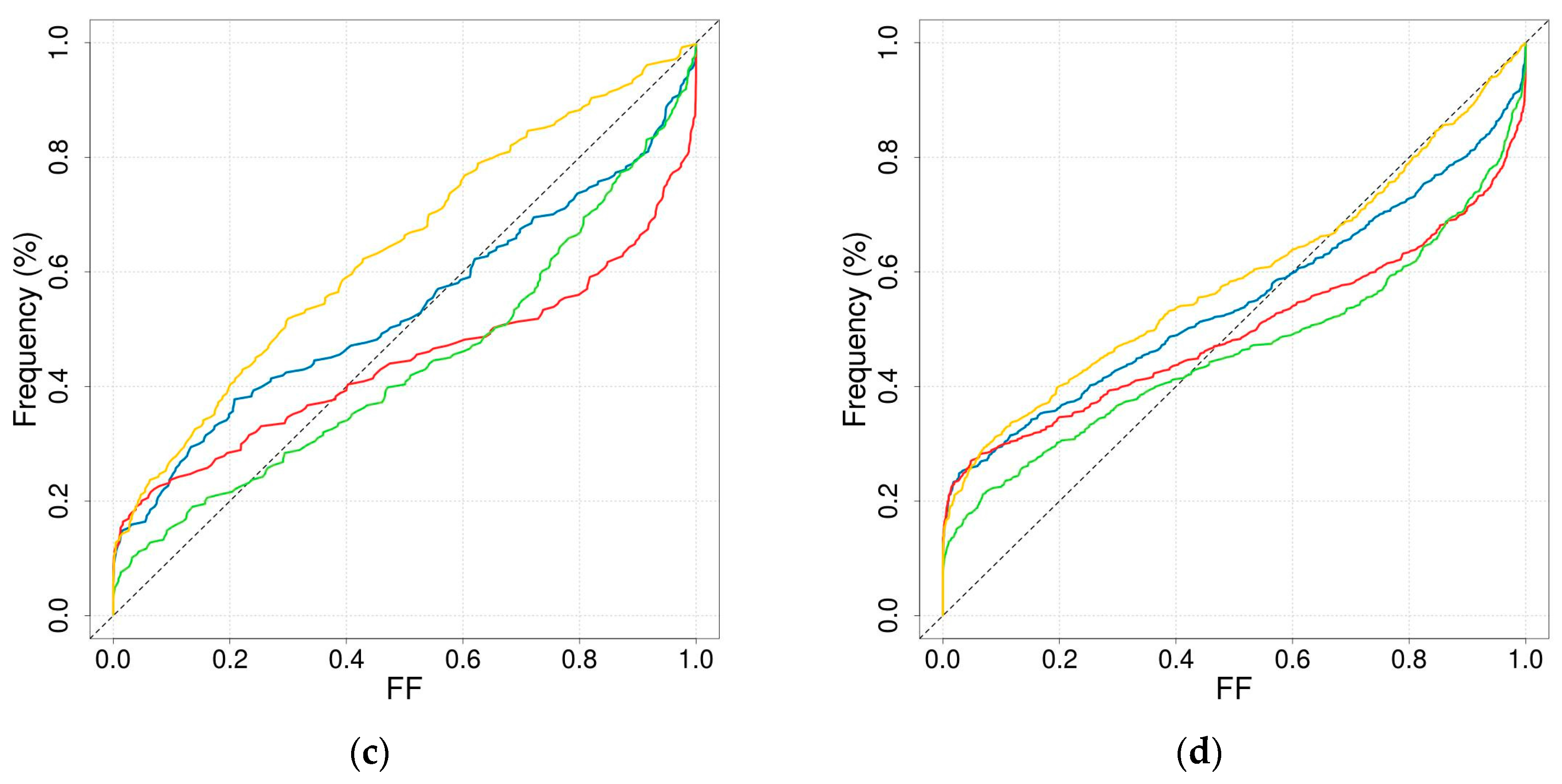
• The FF score evaluates the reliability of the method by analyzing the probability associated by the method to the maximum observed flow.
• The SPAN score evaluates the stability of the method regarding calibration data.

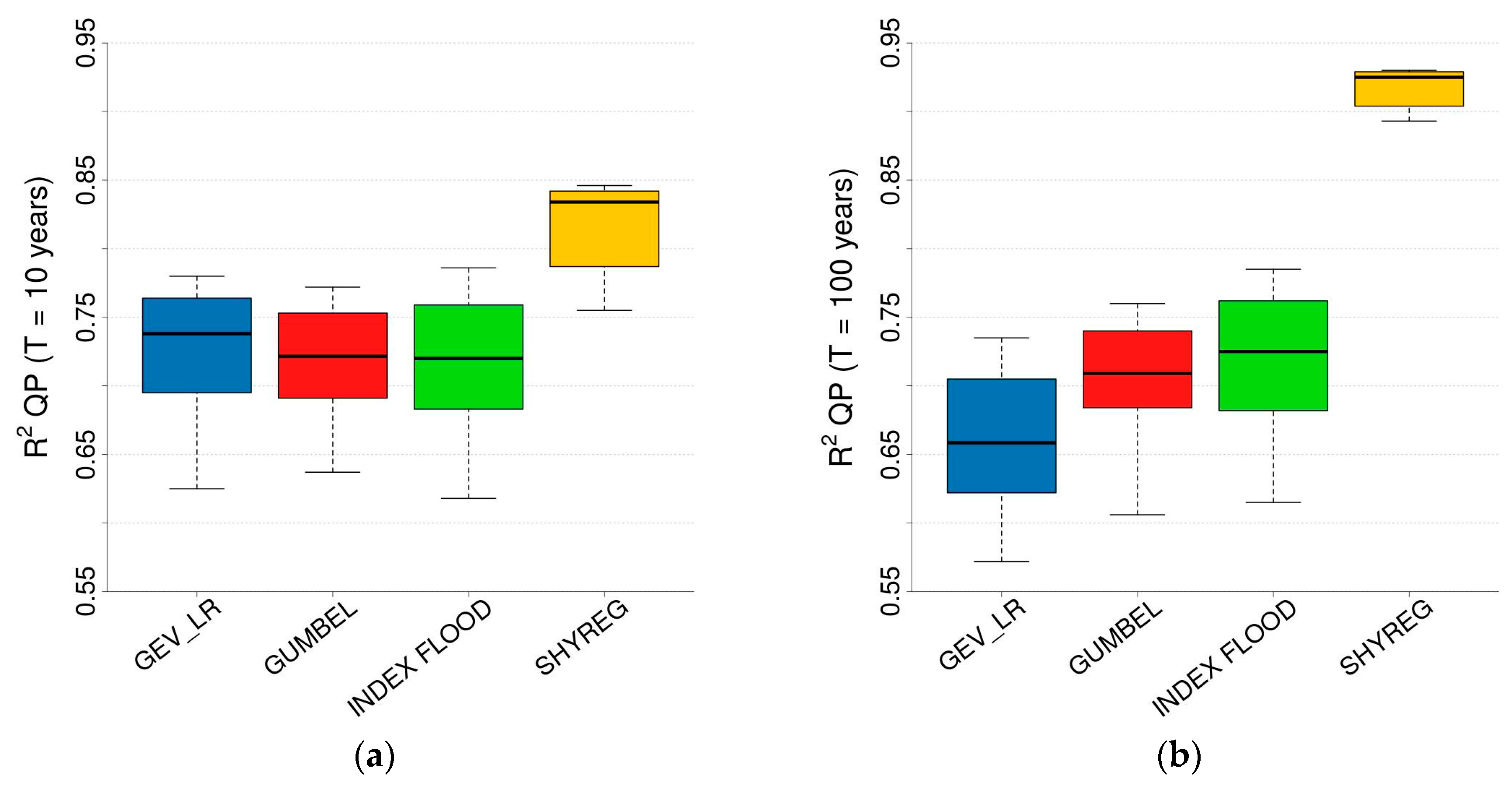
2.4.1. Reproduction of Quantiles

To evaluate the similarity between two sets of quantiles, we calculated the R² coefficient [90] (p. 27), which is described by Equation (8). In this equation, $\widehat{Q}$ is the estimated quantile for a given return period at site i, $Q_{ref}$ is a reference quantile and $\overline{Q_{ref}}$ the average of reference quantiles over the $N$ sites where the evaluation is to be performed. The R² optimal value is 1.

This kind of evaluation has limitations. Indeed, reference quantiles associated with long return periods are a priori difficult to choose. Here, reference quantiles were chosen in two different ways depending on the assessment objectives:

• To assess the accuracy of quantiles associated with low return periods, we assumed that the locally estimated GEV_LR approach is accurate in the observation field (T ≤ 10 years) and is used as a reference to evaluate quantile estimates from other approaches (used in

  Table 3. Criterion values for at-site implementations of the different FFA methods.

  Criterion	Zone	GEV_LR	GUMBEL	INDEX FLOOD	SHYREG
  R2 (T = 10 years)	France	/	0.99	0.94	0.97
  FF	France	0.83	0.93	0.64	0.65
  FF	Mountainous	0.87	0.88	0.71	0.75
  FF	Mediterranean	0.86	0.78	0.61	0.71
  FF	Plains	0.79	0.81	0.61	0.59

  ).
• To assess how well the regionalisation is able to reproduce the quantile estimated locally, the reference quantile of a given FFA is the local quantiles of this FFA. In this case the value of R² does not inform on the accuracy of the regional approach because the quantile evaluated locally can be inaccurate. It can be seen as an evaluation of the stability regarding regionalisation (used in Section 3.2 and Section 3.3.2).

$$R^2=1-\frac{{{\displaystyle \sum }}_{i=1}^N{\left(\widehat{Q}\left(i\right)-Q_{ref}\left(i\right)\right)}^2}{{{\displaystyle \sum }}_{i=1}^N{\left(\widehat{Q}\left(i\right)-\overline{Q_{ref}}\right)}^2}$$

(8)

The R² values were first calculated in a k-fold cross-validation configuration where 90% of the catchments were used as donors to compare the different regionalised FFAs. Then, to study the impact of the river monitoring network density, it was recalculated with successively 80%, 67%, 50% and 33% of the donor catchments.

2.4.2. Reliability of Rare Quantiles

The reliability of the different models for long return periods was evaluated with the FF index [9]. The FF value is actually the probability of non-exceedance associated by the model with the maximum observed flow. With appropriate transformation and under the reliability hypothesis, it can be demonstrated (see [9] for more details) that this value is the realisation of an uniform distribution between 0 and 1. In a probability-probability plot, this theoretical distribution is represented by the first bisector. The idea is to evaluate the deviation between the empirical distribution of the transformed FF values over all the sites and the theoretical one. As described by [9], the shape of the FF distribution around the first bisector in a pp-plot is representative of the behaviour of the model. A curve above the bisector shows a tendency of the model to overestimate the flows, whereas a curve below the bisector is associated with a tendency to underestimate.

A synthetic FF score can be computed as one minus the area between the empirical distribution of FF and its theoretical distribution under the reliability hypothesis (i.e., the first bisector). This optimal value of this FF score is 1.

The FF curves were calculated in a k-fold cross-validation configuration where 90% of the catchments are used as donors.

2.4.3. Stability

The stability of the models regarding calibration data was evaluated with the SPAN index [9]. To calculate this index, it is necessary to evaluate the quantiles at the same catchments from two different data sets. We then compute the SPAN score to assess the difference between the two estimations. The SPAN calculation is described by Equation (9), where $Q_i^T\left(e1\right)$ is the flood quantile of return period T, estimated at the ith site using only dataset e1. The SPAN score is related to the mean absolute relative deviation between two estimations of the same quantile made with two different datasets.

$$SPA{N}_T=1-mean\left(2\frac{\left|Q_i^T\left(e1\right)-Q_i^T\left(e2\right)\right|}{Q_i^T\left(e1\right)+Q_i^T\left(e2\right)}\right)$$

(9)

For the present studies, the catchment set was split into three same-size parts by random selection. The first two parts were used as two different donor sets while the third one was the target set in both cases. We get two different estimations of the quantiles for the catchments in the target set. The process is repeated three times so that each subset is alternatively used as the target set. A synthetic index over the whole catchment set is achieved by calculating one minus the average of the deviations at each site. The optimum of this SPAN score is 1, it indicates that the model reaches the same quantiles estimation whereas it is calibrated with different datasets. Such a model can be considered very stable. Nevertheless, the SPAN score does not evaluate the accuracy of the estimations.

3. Results

3.1. At-Site FFA

The very first step of the study was to calibrate all the FFA implementations for all sites using the whole set of local data. The R² and synthetic FF score resulting from this calibration are presented in Table 3 for the whole study area and discriminated according to the three zones. The GEV_LR approach is used as a reference to calculate the R² values. The R² values suggested good similarity between the estimated 10-year return period quantiles, especially between the GEV_LR and the GUMBEL approaches. This is logical considering they are two distributions from the same family. In addition, the shape parameter mainly influences the upper tail of the distribution and only slightly the 10-year quantile.

One should keep in mind that the FF score values in Table 3 are not a validation. This would require temporal data sampling, as was done in [45,91]. Here the FF score plot only gives insight into the overall behaviour of the methods (tendency to under- or overestimation, over-parameterisation, etc.). In contrast, in the following sections all results are estimations in ungauged sites and are presented for validation catchments.

According to the FF score, the GUMBEL implementation first appeared to be the most satisfactory. Nevertheless, an analysis of the shape of the FF plots (not shown here) over the different zones suggested that the GUMBEL implementation tended to overestimate quantiles for the plains zone and to underestimate them for the mountainous and Mediterranean zones (probably due to the shape parameter imposed at zero, which prevents any heavy-tailed configuration). Other FFAs had a tendency to overestimate extreme quantiles over the whole area. This result could be linked to the use of many catchments with limited time-series (i.e., with quite low maximum observed flow in general).

3.2. Reproduction of At-Site Quantiles

The application of the different regionalisation schemes to the four FFA approaches led to a wide panel of quantile estimations for each catchment. To evaluate the overall capacity of each FFA to be regionalised, we pooled the R² criterion of all the regionalisation techniques implemented. This criterion quantifies the goodness-of-fit between an at-site estimated quantile and the one estimated when the catchment is considered ungauged. The R² value represents the degree of change related to the regionalisation step. The distribution of this criterion for each FFA method is presented on Figure 2. According to this figure, whatever the regionalisation method, the SHYREG quantiles are less affected by the regionalisation process than those from the other three FFAs. In addition, when changing the regionalisation scheme the variability of the R² criterion is lower in the SHYREG case. The difference is greater for 100-year quantiles (Figure 2b) than for 10-year quantiles (Figure 2a). This result shows that even if the regionalisation stage is responsible for a substantial decrease of the quality of the quantiles, the regionalisation method is not the only impacting factor. Actually, some FFA methods, like SHYREG, appear to be more stable regarding regionalisation.

To provide a more in-depth analysis of the different regionalised FFAs, it appears to be necessary to select only one regionalisation technique for each FFA method. This selection is delicate. Indeed, the best method differs depending on the evaluation criterion and the parameter to be regionalised. Consequently, a balance needs to be found between accuracy and stability. In a general way, it can be said that in terms of stability the simplest methods (in terms of the number of parameters) yield the best performance. However, accuracy was better for regionalisation based on both spatial proximity and physical characteristics (i.e., regression with different equations on the regions and/or spatial interpolation of residuals). The final regionalisation selection was made on a case-by-case basis, favouring accuracy over stability, and is a quite subjective step. In all cases, the selected regionalisation schemes are based on different regressions in different regions, and sometimes a spatial interpolation of the residuals seems to be useful. The details of the different regionalisation methods for all the parameters of the FFAs are provided in

Table 4. Description of the selected regionalisation methods for all FFAs and regions.

Region	GEV_LR			Gumbel		Index Flood	SHYREG
	Location	Scale	Shape	Location	Scale	Index	S0/A
Alps-Pyrennees	Rain, grassland, PJ	T, PJ	DT	Rain	T	Rain	AHg, Grassland, rain
Massif Central	NE, forest	NE, PJ, forest	X	NE, forest	PJ, forest	NE, PJ, forest	Forest
East	NE, rain	PJ, Rain	PJ	NE	PJ	NE, Rain	MEDcapa
Mediterranean Arc	DT	DT, PJ, Alt	PJ, rain	DT, PJ, Alt, Snow	PJ, AHg, MEDcapa	DT, PJ, Alt, AHg	MEDcapa, AHg
SE foothills	PJ, area, Y	PJ, DDr, area	Forest, T	PJ	PJ	PJ, DDr, area	Area, Y
Centrals Plains	DDr, NE	DDr, NE	Grassland	DDr, NE	DDr, NE	DDr, NE	DDr
Lorraine Burgundy	DDr, arid	DDr		DDr, arid	DDr, Snow	DDr, arid, grassland	DDr, grassland
Britanny	NE, Y	Y		PJ, Y, HGrock	Y, PJ, HGrock	PJ, Y, HGrock	Arid, Y
Aquitaine	Alt, NE	HGsand, NE		Alt, NE, HGsand	HGsand, NE, area	Alt, area, NE	HGsand, area, Alt
Limousin	DT, AHg	T		DT, AHg	Snow, arid	DT, AHg	PJ, Alt
Spatial interpolation	Yes	Yes	No	Yes	Yes	Yes	No
R2 on parameter over target catchments	0.76	0.72	0.36	0.77	0.70	0.75	0.39

where the descriptors’ names correspond to those in Table 2. We will now consider only the quantiles estimated through the selected regionalisations.

It can be seen in Table 4 that the shape parameter of the GEV_LR and the SHYREG parameter are more difficult to estimate than the others, and in both cases spatial interpolation of the regression residuals was not considered beneficial. It should also be noted that climatic descriptors are mainly selected when regionalising the parameters of the statistical FFA methods. In contrast, few climatic descriptors were selected to explain the variability of the SHYREG parameter. This can be explained because the SHYREG inherently integrates rainfall information. In addition, some descriptors are more selected in certain regions, demonstrating that they are useful to discriminate different hydrological behaviours inside the region. This is the case for the density of drainage networks in the Central plains and Lorraine-Burgundy regions, the rainfall intensity in the SE foothills and Mediterranean arc and also of the presence of sandy soil in the Aquitaine region. In the latter, it is assumed that the HGsand descriptor discriminates the Landes area on the west coast of Aquitaine, which is characterised by a high infiltration of rain water due to the presence of sands. One can also note that the drainage area of the catchment is selected as a descriptor in two regions (SE foothills and Aquitaine). This result is a bit surprising since all discharge data have been reduced by the area according to Equation (1). In fact, the 0.8 coefficient used in Equation (1) might not be the most suitable one for all regions, and the drainage area might keep some explanatory power despite the reduction.

3.3. Comparison of Regionalised FFAs

The comparison of the four regionalised FFAs regarding the three criteria (FF, R², SPAN) are presented on Figure 3, Figure 4 and Figure 5.

3.3.1. Reliability of Rare Quantiles

The FF plots are presented on Figure 3 for all of France and each of the three zones. It should be remembered that the FF criterion is calculated by comparing a model (here a frequency curve estimated by different regionalised FFAs without using at-site data) and observed at-site data. Figure 3 a shows that overall the FFs are quite similar (the area between the FF curves and the first bisector is quite the same) even if some differences in terms of shape are observed. For example, all implementations but SHYREG presented some catchments with an FF value of 1. This value is associated with a model unable to reach a flow as high as the maximum observed flow. Consequently, the tendency of the SHYREG FF curves to catch up to the first bisector for high FF values is a clear advantage. Nevertheless, SHYREG has a tendency to overestimate the quantiles. All implementations had a large number of catchments (around 20%) associated with a null FF value, indicating a frequency curve above the maximum observed flow and consequently a scaling issue in the regionalisation process.

The discrimination of results by zone (Figure 3b–d) is also valuable. Over the plains zone the four implementations show a very similar behaviour as at the national scale. On the other hand, the mountainous and mainly Mediterranean zones discriminate the approaches better. Over the mountainous zone, SHYREG seems to outperform the other approaches by fitting the first diagonal a bit better, whereas the other approaches are qualified by a large number of catchments with FFs at 1 (more than 15% for GUMBEL). Over the Mediterranean zone, the GEV_LR implementation appears to be the most suitable, whereas the GUMBEL implementation appears to be unable to estimate the extreme flows. It can also be noted that the SHYREG implementations tended to overestimate the extreme quantiles, whereas the INDEX FLOOD underestimated them. These results are similar to that obtained in [45] for at-site estimations of daily quantiles (i.e., using the at-site daily discharge data to calibrate the FFA model), but the overall performance is obviously deteriorated by the regionalisation process (i.e., the non-use of at-site discharge data).

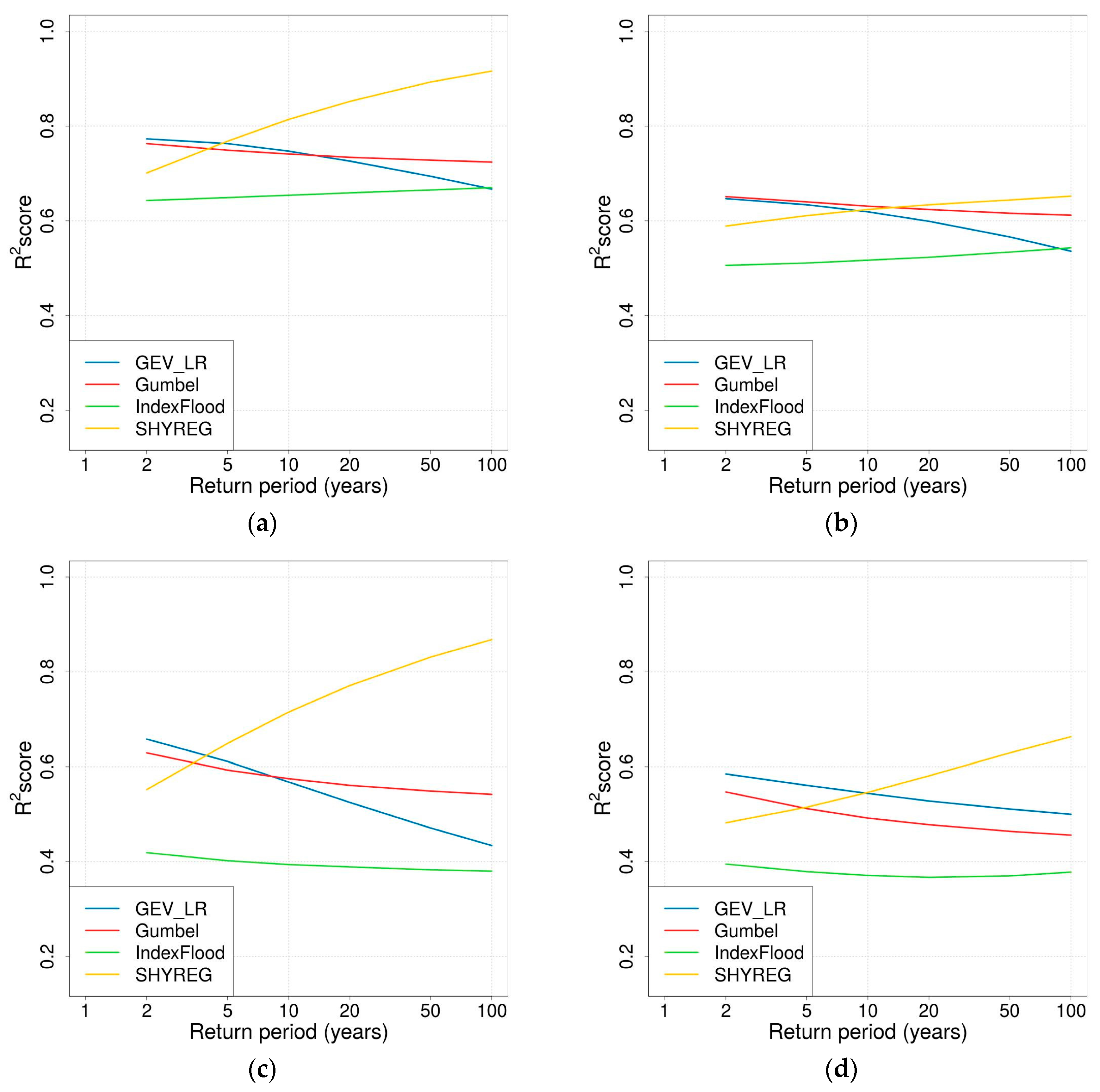
3.3.2. Reproduction of At-Site Estimated Quantiles

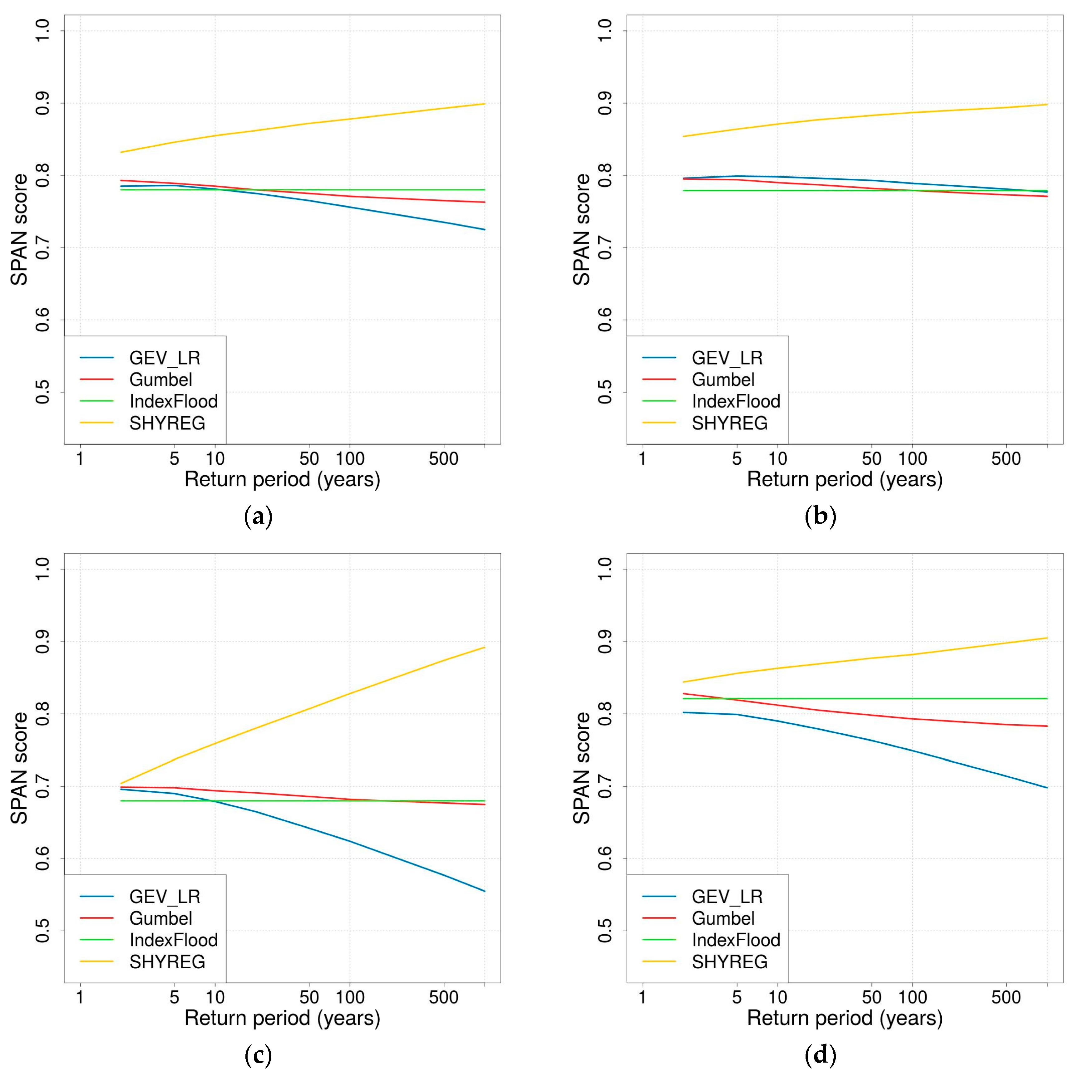
The R² values for all of France and the different zones are exhibited on Figure 4. It should be remembered that the R² criterion evaluates the regionalisation error by comparing quantiles locally estimated with at-site discharge data and quantiles estimated from regionalisation when the catchment is used as the target site and considered ungauged. Graphs are only plotted for return period until 100 years since the reproduction of at-site-estimated quantiles for larger return periods would not be indicative. Figure 4a shows the R² value for all of France. The variability of R² with the return period shows different behaviours. On the one hand, mainly the GEV_LR implementation is characterised by a decreasing R² value with the return period. This can be attributed to the sensitivity of rare quantiles to the shape parameter and the difficulty regionalising this parameter. This hypothesis is confirmed by the relative stability of the GUMBEL and INDEX FLOOD curves for which the shape parameter is not estimated by regionalisation. On the other hand, the R² associated with the SHYREG quantiles increases as the return period increases. This non-intuitive result is due to the structure of the SHYREG model: the calibrated parameter is the initial filling of the production reservoir, so the more extreme the event, the lower the impact of this parameter is. Actually, once the reservoir is saturated, the intensity of flood events only depends on the simulation of rainfall and not at all on the calibrated parameter. Consequently, SHYREG’s long return period quantiles are less sensitive to calibration than frequent quantiles. This effect is even more pronounced over the mountainous (Figure 4d) and mostly Mediterranean regions (Figure 4c) where more intense precipitations are recorded, resulting in more frequent saturation of the production reservoir. In contrast, the GEV_LR, GUMBEL and INDEX FLOOD quantiles are even more sensitive to data sampling in these regions. The plains zone is characterised by a smaller difference between SHYREG and the other regionalised FFAs because precipitation is less likely to saturate the production reservoir.

3.3.3. Stability

The SPAN values are presented on Figure 5. The SPAN reflects the stability of the methods regarding the sampling of donor catchments; it is calculated by comparing the values given by the same model calibrated with two different donor sets. A rapid observation of the four plots on Figure 5 shows that SHYREG is more stable to donor sampling than the other approaches. This result becomes even more obvious if the return period considered is long. This result can be linked to the low dependency between rare SHYREG quantiles and the calibration method (see the explanation of the R² values in the previous section). The other three regionalised FFAs appeared to have very similar stability when calculating the criterion over the whole study area (Figure 5a). When observing the SPAN values for the different sub-zones, it seems that the same observations can be made for the mountainous and plains catchments (Figure 5b). However, the Mediterranean and mountainous area (Figure 5c,d) exhibited a very different behaviour. First of all, Mediterranean catchments are characterised by lower stability of their quantiles estimates whatever the FFA. Then, SHYREG is largely superior to any other implementation in terms of stability, whatever the quantile. The GEV_LR quantiles with a low return period were more stable than those on the high return period, which is an illustration of how difficult it is to calibrate and to regionalise the shape parameter. The stability of GUMBEL and INDEX FLOOD implementations did not seem to be affected by the return period.

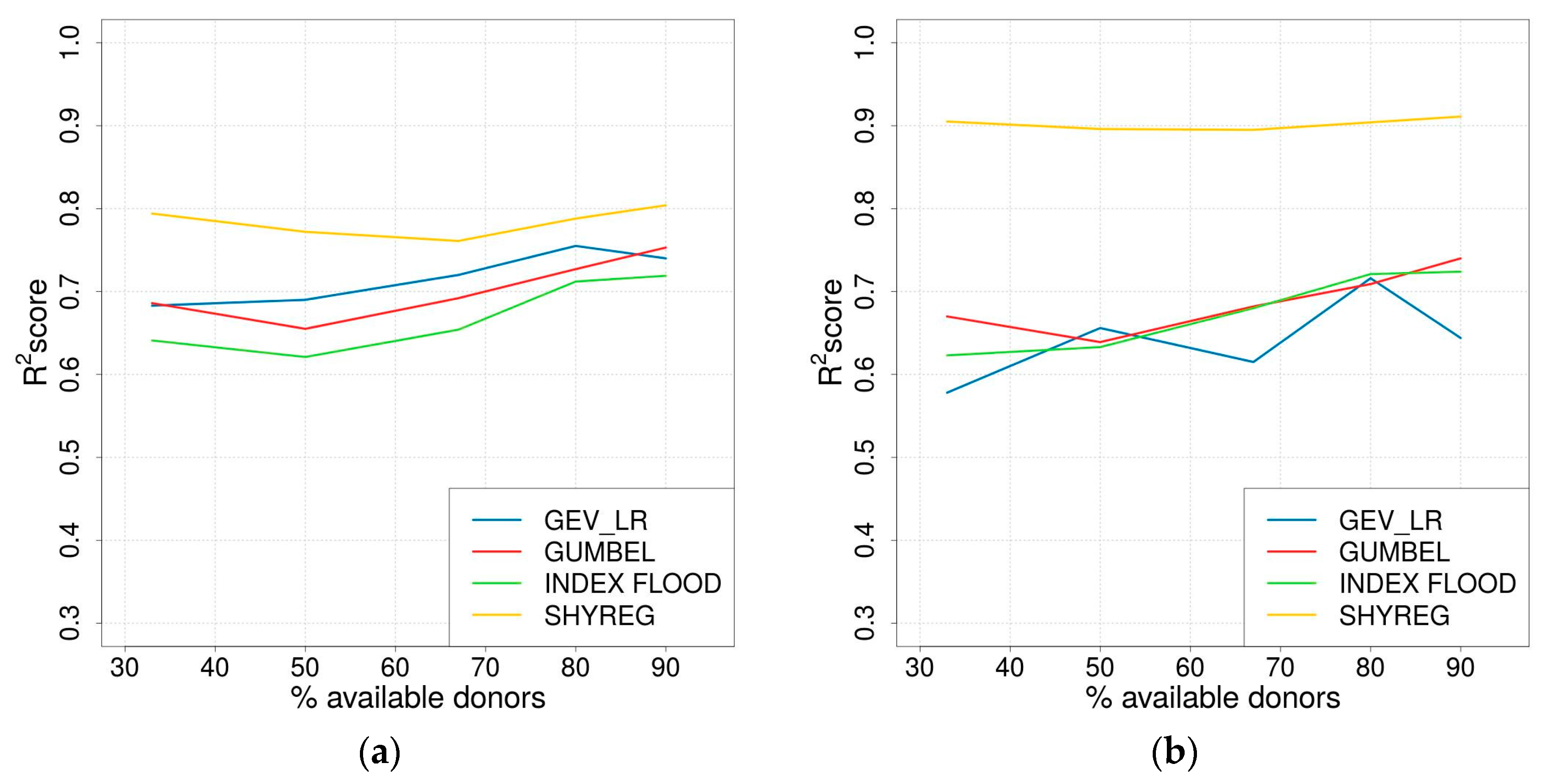
3.4. Impact of the Number of Available Donors

Up to this point, the French hydrological monitoring network was used as much as possible to calibrate and regionalise the FFAs. Nevertheless, the use of the very dense network could limit the generalisation of the results presented to other study areas. Therefore, the different regionalised FFAs were calibrated and regionalised using only a fraction of the available donor catchments (k-fold analysis). For each FFA, the same regionalisation scheme was employed (identical to the previous cases), whatever the number of available donors. Figure 6 shows the R² criterion calculated for each regionalised FFA using only a percentage of the available donors. For better readability, only the R² values associated with the 10-year and 100-year quantiles are presented. It can be noted that the case using 90% of the catchments as donors is the one presented in the previous sections.

Figure 6 shows that the GEV_LR, GUMBEL and INDEX FLOOD experienced some R² loss due to the decrease of available donors. For the GEV_LR implementation, this loss is even more visible for high return period quantiles (1000-year quantiles). It can also be seen that the criterion values are not systematically ranked according to the number of available donors; this was attributed to random regionalisation error, and we assumed that a more systemic approach (performing numerous re-samplings of the donors) would attenuate this effect. The SHYREG implementation suffered less from the decrease in donor availability: an R² criterion loss was only observed for low return period quantiles (10-year quantiles), which again illustrates that extreme SHYREG quantiles rely mostly on rainfall simulation and not on calibration against discharge data.

4. Discussion

From the different results exhibited here it can be claimed that the SHYREG simulation-based approach exhibits behaviour quite different from the three other FFA methods tested. This is actually not surprising due to the structural differences between the methods. SHYREG is a simulation-based process based on the generation of numerous rainy and flood events, whereas the others perform probability distribution fitting over discharge data.

The main differences exhibited in the previous section can be related to the behaviour towards the long return periods of the different approaches tested:

• In the SHYREG simulation, the only parameter calibrated against discharge data is the initial filling of the production reservoir. This parameter was not very well estimated by regionalisation. The reservoir can become saturated for extreme floods; consequently, the most extreme events simulated by SHYREG does not strongly depend on the calibrated parameter. This means that in the SHYREG simulation the calibration is used to position the start of the frequency curve (i.e., low return periods), whereas the asymptotic behaviour is based almost completely on the rainfall simulation. Consequently, the upper tail of the simulated distribution is only slightly affected by regionalisation errors (contrary to the lower tail). This point explains why the stability of the regionalised SHYREG quantiles appears to increase as the return period increases (very stable extreme quantile and variable frequent quantiles), and why these extreme regionalised quantiles are very similar to the calibrated quantiles. In addition, thanks to an extensive work on rainfall analysis [47,76,92,93], SHYREG benefits from an accurate rainfall information [78] even in ungauged sites. It is not the case for other approaches, and it makes it less dependent its regionalised parameter.
• The asymptotic behaviour of a GEV distribution is highly controlled by the shape parameter. Not only is this parameter challenging to estimate using at-site data because it is very sensitive to sampling, but it is also more difficult to regionalise than the other two (the second issue can probably be related to the first one). This means that the upper tail of the flood distribution suffers significantly from regionalisation errors. This is the reason why the stability of GEV_LR-estimated quantiles appears to decrease when considering longer return periods.
• In the GUMBEL approach, a null shape parameter is imposed. Consequently, the shape of the flood distribution, and especially its skewness, remains quite stable even during the regionalisation process. Nevertheless, the GUMBEL distribution is not flexible enough to describe the dynamics of the most responsive catchments (i.e., Mediterranean catchments), which can explain why it has a tendency to underestimate extreme quantiles over the Mediterranean zone.
• The INDEX FLOOD approach is supposed to overcome the issues of stability (exhibited by the GEV_LR implementation) and flexibility (exhibited by the GUMBEL case) by considering regional distribution and local scaling indexes. Its stability does not depend on the return period considered. The comparison of the growth curves between the regions actually shows heavier upper tails for the Mediterranean and mountainous regions than for the plains. Nevertheless, in the end this approach underwent more losses during the regionalisation stages, leading to quite poor performance. This approach may have suffered from a lack of development already visible at the calibration stage. A more in-depth analysis of the definition of the regions and at-site performance would probably be necessary to enhance the performance of this method.

Another difference is related to the need to estimate multiple quantiles. This then requires respecting several constraints between the quantiles:

• Consistency between quantiles in terms of return period to estimate the entire flood frequency curve for a return period up to 1000 years;
• Consistency between quantiles in terms of time-steps to estimate maximum flow quantiles of different durations;
• Spatial consistency when several target catchments are considered, even if the spatial coherence of the estimated quantiles between the different sites was not analysed here.

This multiplicity of the requirements for consistency resulted in ruling out or criticising certain approaches. For example, if estimating a single quantile is the objective, then it could be appropriate to regionalise quantiles directly instead of parameters [25]. Nevertheless, if multiple return periods are of interest, it appears more reasonable to choose a parameter regionalisation over a quantile regionalisation scheme. Similarly, one should opt for a method taking into account the different quantiles’ dependency (an example using copulas can be found in [94]). Not doing this might not lead to poorer overall performance, but locally some inconsistencies might be difficult to manage. However, this solution would increase the number of models and parameters to calibrate and regionalise, possibly at the cost of stability. Another way of forcing coherency is to do it in the regionalisation step using, for example, regression with the same descriptors to regionalise the quantiles [39,41].

A similar issue might arise when considering multiple time-step quantiles. Here we focused on peak flows but other time steps can be of interest, especially for small catchments where these different quantiles can differ greatly. The SHYREG method produces quantiles of different time steps which are coherent because they are extracted from hydrographs. With the GEV_LR, GUMBEL and INDEX FLOOD, it would be necessary to proceed to a second application of both FFA and regionalisation. A similar approach was applied to daily flows instead of peak flows, resulting in a ratio of peak over daily flow reaching impossible values (i.e., below 1) for around 4% of the catchments with the statistical FFAs. This issue was not observed with SHYREG because it structurally considers a dependency between time-steps. An alternative solution could also be to use a method taking into account time-step dependency. However, again, such a solution might increase the complexity of the method and can impact its stability.

5. Conclusions

The main results of the present study can be summarised in the following points:

• The regionalisation process is the source of substantial loss of performance in FFA. Consequently, stability regarding at-site calibration data is a very valuable advantage for regionalisation. For this reason, the process-based methods, such as SHYREG, appear to be a safe solution method for flood estimation in ungauged basins.
• Methods that do not take into account the dependency between quantiles (between the different return periods and/or time-steps) can lead to incoherent flood frequency estimation. Therefore, when interested in multiple quantile estimations one should explicitly consider these dependencies or employ an approach that does: for example, parameter regionalisation rather than quantile regionalisation.
• The results can vary greatly depending on the study area. When studying a large and variable area, discrimination by region is necessary to analyse the results. In France, the Mediterranean region should at least be considered separately.
• In the present case, for a long return period, the low dependence between the regionalised SHYREG extreme quantiles and calibration discharge data provide quantile estimates relatively close to that obtained in a gauged configuration, i.e., quantiles that can be and have already been validated [18,45].
• Due to its low dependence on calibration, the SHYREG method appeared to be less affected by decreasing the number of available gauging stations. Nevertheless, the SHYREG quantiles largely rely on previous rainfall simulations [47,76,78]; consequently, an application to other areas would still require the availability of rainfall data sets.

The association of an FFA with a regionalisation scheme and different validation configurations necessarily leads to a wide panel of implementations. Consequently, choices and simplifications were needed to conduct the present study. One could imagine reinforcing the comparison framework by performing data re-samplings (temporal and/or spatial). It could also be beneficial to consider diverse improvements of the different FFAs to correct some of the weaknesses identified here. Nevertheless, the present study allows exhibiting the fundamental differences between the different approaches for flood frequency estimation in ungauged catchments.

References

1. Ministère de la Transition Écologique et Solidaire. Prévention des Inondations. Available online: http://www.developpement-durable.gouv.fr/prevention-des-inondations (accessed on 18 May 2017).
2. Castellarin, A.; Kohnová, S.; Gaál, L.; Fleig, A.; Salinas, J.L.; Toumazis, A.; Kjeldsen, T.R.; Macdonald, N. Review of Applied-Statistical Methods for Flood-Frequency Analysis in Europe: WG2 of Cost Action ES0901; Castellarin, A., Kohnová, S., Gaál, L., Fleig, A., Salinas, J.L., Toumazis, A., Kjeldsen, T.R., Macdonald, N., Eds.; The Centre for Ecology & Hydrology: Lancashire, UK, 2012. [Google Scholar]
3. Willems, P.; Blazkova, S.; Beven, K.J.; Arnaud, P.; Paquet, E.; Loukas, A.; Vasiliades, L.; Efstratiadis, A.; Lawrence, D.; Szolgay, J.; et al. Rewiew of European Simulation Methods for Flood-Frequency-Estimation. WG3: Flood Frequency Analysis Using Rainfall-Runoff Methods; Willems, P., Blazkova, S., Beven, K.J., Arnaud, P., Paquet, E., Loukas, A., Vasiliades, L., Efstratiadis, A., Lawrence, D., Szolgay, J., Eds.; Report of Cost Action, ES0901; The Centre for Ecology & Hydrology: Lancashire, UK, 2012. [Google Scholar]
4. Katz, R.W.; Parlange, M.B.; Naveau, P. Statistics of extremes in hydrology. Adv. Water Resour. 2002, 25, 1287–1304. [Google Scholar] [CrossRef]
5. Prescott, P.; Walden, A.T. Maximum likelihood estimation of the parameters of the generalized extreme-value distribution. Biometrika 1980, 67, 723–724. [Google Scholar] [CrossRef]
6. Hosking, J.R.M.; Wallis, J.R.; Wood, E.F. Estimation of the generalized extreme-value distribution by the method of probability-weighted moments. Technometrics 1985, 27, 251–261. [Google Scholar] [CrossRef]
7. Martins, E.S.; Stedinger, J.R. Generalized maximum-likelihood generalized extreme-value quantile estimators for hydrologic data. Water Resour. Res. 2000, 36, 737–744. [Google Scholar] [CrossRef]
8. Kuczera, G. Comprehensive at-site flood frequency analysis using monte carlo bayesian inference. Water Resour. Res. 1999, 35, 1551–1557. [Google Scholar] [CrossRef]
9. Renard, B.; Kochanek, K.; Lang, M.; Garavaglia, F.; Paquet, E.; Neppel, L.; Najib, K.; Carreau, J.; Arnaud, P.; Aubert, Y.; et al. Data-based comparison of frequency analysis methods: A general framework. Water Resour. Res. 2013, 49, 825–843. [Google Scholar] [CrossRef] [Green Version]
10. Ribatet, M.; Sauquet, E.; Grésillon, J.M.; Ouarda, T.B.M.J. A regional bayesian pot model for flood frequency analysis. Stoch. Environ. Res. Risk Assess. 2007, 21, 327–339. [Google Scholar] [CrossRef]
11. Hosking, J.R.M.; Wallis, J.R. Regional Frequency Analysis: An Approach Based on L-Moments; Cambridge University Press: Cambridge, UK, 1997. [Google Scholar]
12. Stedinger, J.R. Estimating a regional flood frequency distribution. Water Resour. Res. 1983, 19, 503–510. [Google Scholar] [CrossRef]
13. Dalrymple, T. Flood-Frequency Analyses, Manual of Hydrology: Part 3; 1543A; United States Government Publishing Office: Washington, WA, USA, 1960.
14. Renard, B. A bayesian hierarchical approach to regional frequency analysis. Water Resour. Res. 2011, 47. [Google Scholar] [CrossRef]
15. Li, J.; Thyer, M.; Lambert, M.; Kuczera, G.; Metcalfe, A. An efficient causative event-based approach for deriving the annual flood frequency distribution. J. Hydrol. 2014, 510, 412–423. [Google Scholar] [CrossRef]
16. Blazkova, S.; Beven, K. Flood frequency estimation by continuous simulation of subcatchment rainfalls and discharges with the aim of improving dam safety assessment in a large basin in the Czech Republic. J. Hydrol. 2004, 292, 153–172. [Google Scholar] [CrossRef]
17. Eagleson, P.S. Dynamics of flood frequency. Water Resour. Res. 1972, 8, 878–898. [Google Scholar] [CrossRef]
18. Arnaud, P.; Cantet, P.; Aubert, Y. Relevance of an at-site flood frequency analysis method for extreme events based on stochastic simulation of hourly rainfall. Hydrol. Sci. J. 2016, 61, 36–49. [Google Scholar] [CrossRef]
19. Paquet, E.; Garavaglia, F.; Garçon, R.; Gailhard, J. The schadex method: A semi-continuous rainfall-runoff simulation for extreme flood estimation. J. Hydrol. 2013, 495, 23–37. [Google Scholar] [CrossRef]
20. Blöschl, G.; Sivapalan, M. Scale issues in hydrological modelling: A review. Hydrol. Process. 1995, 9, 251–290. [Google Scholar] [CrossRef]
21. Stedinger, J.R.; Tasker, G.D. Regional hydrologic analysis: 1. Ordinary, weighted, and generalized least squares compared. Water Resour. Res. 1985, 21, 1421–1432. [Google Scholar] [CrossRef]
22. Gupta, V.K.; Mesa, O.J.; Dawdy, D.R. Multiscaling theory of flood peaks: Regional quantile analysis. Water Resour. Res. 1994, 30, 3405–3421. [Google Scholar] [CrossRef]
23. Skøien, J.O.; Merz, R.; Blöschl, G. Top-kriging—Geostatistics on stream networks. Hydrol. Earth Syst. Sci. 2006, 10, 277–287. [Google Scholar] [CrossRef]
24. Micevski, T.; Hackelbusch, A.; Haddad, K.; Kuczera, G.; Rahman, A. Regionalisation of the parameters of the log-Pearson 3 distribution: A case study for New South Wales, Australia. Hydrol. Process. 2015, 29, 250–260. [Google Scholar] [CrossRef]
25. Haddad, K.; Rahman, A.; Stedinger, J.R. Regional flood frequency analysis using bayesian generalized least squares: A comparison between quantile and parameter regression techniques. Hydrol. Process. 2012, 26, 1008–1021. [Google Scholar] [CrossRef]
26. Ahn, K.H.; Palmer, R. Regional flood frequency analysis using spatial proximity and basin characteristics: Quantile regression vs. Parameter regression technique. J. Hydrol. 2016, 540, 515–526. [Google Scholar] [CrossRef]
27. Organde, D.; Arnaud, P.; Fine, J.A.; Fouchier, C.; Folton, N.; Lavabre, J. Regionalization of a flood frequency estimation method over Metropolitan France: The shyreg method. Revue des Sciences de l'Eau 2013, 26, 65–78. [Google Scholar] [CrossRef]
28. Basu, B.; Srinivas, V.V. Evaluation of the index-flood approach related regional frequency analysis procedures. J. Hydrol. Eng. 2016, 21. [Google Scholar] [CrossRef]
29. Hailegeorgis, T.T.; Alfredsen, K. Regional flood frequency analysis and prediction in ungauged basins including estimation of major uncertainties for mid-Norway. J. Hydrol. Reg. Stud. 2017, 9, 104–126. [Google Scholar] [CrossRef]
30. Sefton, C.E.M.; Howarth, S.M. Relationships between dynamic response characteristics and physical descriptors of catchments in England and Wales. J. Hydrol. 1998, 211, 1–16. [Google Scholar] [CrossRef]
31. Seibert, J. Regionalisation of parameters for a conceptual rainfall-runoff model. Agric. For. Meteorol. 1999, 98, 279–293. [Google Scholar] [CrossRef]
32. Burn, D.H. Evaluation of regional flood frequency analysis with a region of influence approach. Water Resour. Res. 1990, 26, 2257–2265. [Google Scholar] [CrossRef]
33. Burn, D.H. An appraisal of the “region of influence” approach to flood frequency analysis. Hydrol. Sci. J. 1990, 35, 149–165. [Google Scholar] [CrossRef]
34. Vandewiele, G.L.; Elias, A. Monthly water balance of ungauged catchments obtained by geographical regionalization. J. Hydrol. 1995, 170, 277–291. [Google Scholar] [CrossRef]
35. Oudin, L.; Andréassian, V.; Perrin, C.; Michel, C.; Le Moine, N. Spatial proximity, physical similarity, regression and ungaged catchments: A comparison of regionalization approaches based on 913 French catchments. Water Resour. Res. 2008, 44, W03413. [Google Scholar] [CrossRef]
36. Merz, R.; Blöschl, G. Flood frequency regionalisation—Spatial proximity vs. Catchment attributes. J. Hydrol. 2005, 302, 283–306. [Google Scholar] [CrossRef]
37. Kjeldsen, T.R.; Jones, D.A.; Bayliss, A.C. Improving the Floof Estimation Handbook (FEH) Statistical Procedures for Flood Frequency Estimation; SCHO0608BOFF-E; Environment Agency: Bristol, UK, 2008.
38. Robson, A.J.; Reed, D.W. Floord Estimation Handbook Vol. 3: Statistical Procedures for Flood Frequency Estimation; Institute of Hydrology: Wallingford, UK, 1999; p. 338. [Google Scholar]
39. Mateo Lázaro, J.; Sánchez Navarro, J.Á.; García Gil, A.; Edo Romero, V. Flood frequency analysis (FFA) in spanish catchments. J. Hydrol. 2016, 538, 598–608. [Google Scholar] [CrossRef]
40. United States Geological Survey (USGS). Guidelines for Determining Flood Flow Frequency: Bulletin 17B of the Hydrology Subcomittee; United States Geological Survey: Reston, VA, USA, 1982.
41. Jennings, M.E.; Thomas, W.O.; Riggs, H.C. Nationwide Summary of U.S. Geological Survey Regional Regression Equations for Estimating Magnitude and Frequency of Floods for Ungaged Sites; United States Geological Survey: Reston, VA, USA, 1993.
42. Ball, J.; Weinmann, E.; Kuczera, G. Peak flow estimation. In Australian Rainfall and Runoff: A Guide to Flood Estimation; Ball, J., Babister, M., Nathan, R.J., Weeks, W., Weinmann, E., Retallick, M., Testoni, I., Eds.; Commonwealth of Australia: Canberra, Australia, 2016; Volume 3. [Google Scholar]
43. Ball, J.; Weinmann, E. Flood hydrograph estimation. In Australian Rainfall and Runoff: A Guide to Flood Estimation; Ball, J., Babister, M., Nathan, R.J., Weeks, W., Weinmann, E., Retallick, M., Testoni, I., Eds.; Commonwealth of Australia: Canberra, Australia, 2016; Volume 5. [Google Scholar]
44. Beven, K.J. Rainfall-Runoff Modeling: The Primer; John Wiley & Sons Ltd.: Chichester, UK, 2001. [Google Scholar]
45. Kochanek, K.; Renard, B.; Arnaud, P.; Aubert, Y.; Lang, M.; Cipriani, T.; Sauquet, E. A data-based comparison of flood frequency analysis methods used in France. Nat. Hazards Earth Syst. Sci. 2014, 14, 295–308. [Google Scholar] [CrossRef] [Green Version]
46. Aubert, Y.; Arnaud, P.; Ribstein, P.; Fine, J.A. The SHYREG flow method-application to 1605 basins in Metropolitan France. Hydrol. Sci. J. 2014, 59, 993–1005. [Google Scholar] [CrossRef]
47. Arnaud, P.; Lavabre, J. Coupled rainfall model and discharge model for flood frequency estimation. Water Resour. Res. 2002, 38, 11-1–11-11. [Google Scholar] [CrossRef]
48. Ministère de l’Écologie du Développement Durable et de l’Energie. Banque hydro. Ministère de l’Ecologie du Dévelopement Durable et de l’Energie, SCHAPI. Available online: http://www.hydro.eaufrance.fr/ (accessed on 18 September 2017).
49. McDonald, J.H. Handbook of Biological Statistics; Sparky House Publishing: Baltimore, MD, USA, 2009; Volume 2. [Google Scholar]
50. Vidal, J.P.; Martin, E.; Franchistéguy, L.; Baillon, M.; Soubeyroux, J.M. A 50-year high-resolution atmospheric reanalysis over France with the safran system. Int. J. Climatol. 2010, 30, 1627–1644. [Google Scholar] [CrossRef] [Green Version]
51. Budyko, M.I. The Heat Balance of the Earth’s Surface; U.S. Department of Commerce, Weather Bureau: Washington, DC, USA, 1958; 259p.
52. Aubert, Y. Estimation des Valeurs Extrêmes de Débit par la Méthode Shyreg: Réflexions sur L’équifinalité dans la Modélisation de la Transformation Pluie en Débit. Ph.D. Thesis, Université Pierre et Marie Curie, Paris, France, 2012. [Google Scholar]
53. Sol, B.; Desouches, C. Spatialisation à Résolution Kilométrique sur la France de Paramètres liés aux Précipitations; Rapport d’étude Météo-France; Convention Météo-France DPPR n 03/1735; Météo-France: Toulouse, France, 2015; 41p. [Google Scholar]
54. IGN; ONEMA. BD Carthage. Available online: http://professionnels.ign.fr/bdcarthage (accessed on 18 September 2017).
55. European Union Agency. European Digital Elevation Model (EU-DEM), 1st ed.; Copernicus, 2016; Available online: http://land.copernicus.eu/pan-european/satellite-derived-products/eu-dembdcarthage (accessed on 18 September 2017).
56. Margat, J. Carte Hydrogéologique de la France: Systèmes Aquifères; BRGM: Orléans, France, 1978. [Google Scholar]
57. Finke, P.; Hartwich, R.; Dudal, R.; Ibanez, J.; Jamagne, M.; King, D.; Montanarella, L.; Yassoglou, N. Geo-Referenced Soil Database for Europe. In Manual of Procedures, version 1.0; European Commission, 1998; Available online: https://www.researchgate.net/publication/254560058_Georeferenced_Soil_Database_for_Europe_Manual_of_Procedures_Version_10 (accessed on 18 September 2017).
58. European Union SOeS. Corine Land Cover (CLC) 2012; Service de l’Observation et des statistiques (SOeS) du Commissariat Général au Développement Durable du MEDDE, 2012; Available online: http://www.statistiques.developpement-durable.gouv.fr/donnees-ligne/li/1825.html (accessed on 18 September 2017).
59. Wasson, J.G.; Chandesris, A.; Pella, H.; Blanc, L. Les Hydro-Écorégions de France Métropolitaine. Approche Régionale de la Typologie des Eaux Courantes et Éléments Pour la Définition des Peuplements de Référence D'invertébrés; Ministère de l’Écologie et du Développement Durable, Cemagref BEA/LHQ, 2002; p. 190. Available online: http://www.irstea.fr/la-recherche/unites-de-recherche/maly/pole-onema-irstea/regionalisation-et-typologie/les-hydro (accessed on 18 September 2017).
60. Cipriani, T.; Toilliez, T.; Sauquet, E. Estimating 10 year return period peak flows and flood durations at ungauged locations in France. Houille Blanche 2012, 4–5, 5–13. [Google Scholar] [CrossRef]
61. Garcia, F. Amélioration d’une Modélisation Hydrologique Régionalisée Pour Estimer les Statistiques D’étiage. Ph.D. Thesis, Université Pierre et Marie Curie, Paris, France, 2016. [Google Scholar]
62. Hijmans, R.J.; Van Etten, J. Raster: Geographic Data Analysis and Modeling, R Package Version 2.5-8; 2014. Available online: https://CRAN.R-project.org/package=raster (accessed on 18 September 2017).
63. R Core Team. R: A Language and Environment for Statistical Computing; R Foundation for Statistical Computing: Vienna, Austria, 2016. [Google Scholar]
64. Lê, S.; Josse, J.; Husson, F. Factominer: An R package for multivariate analysis. J. Stat. Softw. 2008, 25. [Google Scholar] [CrossRef]
65. Coles, S. An Introduction to Statistical Modeling of Extreme Values; Springer: Heidelberg, Germany, 2001. [Google Scholar]
66. Geyer, C.; Johnson, L. Mcmc: Markov Chain Monte Carlo, R Package Version 0.9-4; Available online: https://CRAN.R-project.org/package=mcmc (accessed on 18 September 2017).
67. Stephenson, A.G. Evd: Extreme value distributions. R News 2002, 2, 31–32. [Google Scholar]
68. Hosking, J.R.M.; Wallis, J.R. Some statistics useful in regional frequency analysis. Water Resour. Res. 1993, 29, 271–281. [Google Scholar] [CrossRef]
69. Stedinger, J.R.; Lu, L.H. Appraisal of regional and index flood quantile estimators. Stoch. Hydrol. Hydraul. 1995, 9, 49–75. [Google Scholar] [CrossRef]
70. Gaume, E.; Gaál, L.; Viglione, A.; Szolgay, J.; Kohnová, S.; Blöschl, G. Bayesian mcmc approach to regional flood frequency analyses involving extraordinary flood events at ungauged sites. J. Hydrol. 2010, 394, 101–117. [Google Scholar] [CrossRef]
71. Kjeldsen, T.R. Flood Estimation Handbook Supplementary Report No. 1: The Revitalised FSR/FEH Rainfall-Runioff Method; Centre for Ecology & Hydrology: Wallingford, UK, 2007. [Google Scholar]
72. Oudin, L.; Kay, A.; Andráassian, V.; Perrin, C. Are seemingly physically similar catchments truly hydrologically similar? Water Resour. Res. 2010, 46. [Google Scholar] [CrossRef]
73. Cernesson, F. Modèle Simple de Prédetermination des Crues de Fréquences Courantes à Rares sur Petits Bassins Versants Méditéranéens. Ph.D. Thesis, Université Montpellier II, Montpellier, France, 1993. [Google Scholar]
74. Arnaud, P. Modèle de Prédétermination de Crues Basé sur la Simulation. Extension de sa Zone de Validité, Paramétrisation du Modèle Horaire par L’information Journalière et Couplage des Deux pas de Temps. Ph.D. Thesis, Université Montpellier II, Montpellier, France, 1997. [Google Scholar]
75. Cantet, P. Impacts du Changement Climatique sur les Pluies Extrêmes par L’utilisation d’un Générateur Stochastique de Pluies. Ph.D. Thesis, Université Montpellier II, Montpellier, France, 2009. [Google Scholar]
76. Cantet, P.; Arnaud, P. Gains from modelling dependence of rainfall variables into a stochastic model: Application of the copula approach at several sites. Hydrol. Earth Syst. Sci. Discuss. 2012, 9, 11227–11266. [Google Scholar] [CrossRef]
77. Arnaud, P.; Lavabre, J.; Sol, B.; Desouches, C. Cartographie de l’aléa pluviographique de la France. La Houille Blanche 2006, 5, 102–111. [Google Scholar] [CrossRef]
78. Carreau, J.; Neppel, L.; Arnaud, P.; Cantet, P. Extreme rainfall analysis at ungauged sites in the south of France: Comparison of three approaches. J. Soc. Fr. Stat. 2013, 154, 119–138. [Google Scholar]
79. Arnaud, P.; Lavabre, J. Estimation de L’aléa Pluvial en France Métropolitaine; QUAE; Update Sciences & Technologies: Paris, France, 2010; 158p. [Google Scholar]
80. IRSTEA. Catchment Hydrology Research Group. Available online: https://webgr.irstea.fr/ (accessed on 18 September 2017).
81. Coron, L.; Perrin, C.; Delaigue, O.; Andréassian, V.; Thirel, G. airGR: A suite of lumped hydrological models in an R-package. Environ. Model. Softw. 2017, in press. [Google Scholar] [CrossRef]
82. Parajka, J.; Merz, R.; Blöschl, G. A comparison of regionalisation methods for catchment model parameters. Hydrol. Earth Syst. Sci. 2005, 9, 157–171. [Google Scholar] [CrossRef]
83. Kokkonen, T.S.; Jakeman, A.J.; Young, P.C.; Koivusalo, H.J. Predicting daily flows in ungauged catchments: Model regionalization from catchment descriptors at the coweeta hydrologic laboratory, North Carolina. Hydrol. Process. 2003, 17, 2219–2238. [Google Scholar] [CrossRef]
84. McIntyre, N.; Lee, H.; Wheater, H.; Young, A.; Wagener, T. Ensemble predictions of runoff in ungauged catchments. Water Resour. Res. 2005, 41. [Google Scholar] [CrossRef]
85. Zhang, Y.; Chiew, F.H.S. Relative merits of different methods for runoff predictions in ungauged catchments. Water Resour. Res. 2009, 45. [Google Scholar] [CrossRef]
86. Beck, H.E.; van Dijk, A.I.J.M.; de Roo, A.; Miralles, D.G.; McVicar, T.R.; Schellekens, J.; Bruijnzeel, L.A. Global-scale regionalization of hydrologic model parameters. Water Resour. Res. 2016, 52, 3599–3622. [Google Scholar] [CrossRef] [Green Version]
87. Thomas, D.M.; Benson, M.A. Generalization of Streamflow Characteristics from Drainage-Basin Characteristics; United States Government Printing Office: Washington, DC, USA, 1975.
88. Tasker, G.D.; Hodge, S.A.; Barks, C.S. Region of influence regression for estimating the 50-year flood at ungaged sites. J. Am. Water Resour. Assoc. 1996, 32, 163–170. [Google Scholar] [CrossRef]
89. Akaike, H. A new look at the statistical model identification. IEEE Trans. Autom. Control 1974, 19, 716–723. [Google Scholar] [CrossRef]
90. Blöschl, G.; Sivapalan, M.; Wagener, T.; Viglione, A.; Savenije, H. Runoff Prediction in Ungauged Basins: Synthesis across Processes, Places and Scales; Blöschl, G., Sivapalan, M., Wagener, T., Viglione, A., Savenije, H., Eds.; Cambridge University Press: Cambridge, UK, 2013; pp. 1–465. [Google Scholar]
91. Arnaud, P. L’aléa Hydrométéorologique: Estimation Régionale par Simulation Stochastique des Processus; HDR; Aix Marseille Université: Aix en Provence, France, 2015. [Google Scholar]
92. Arnaud, P.; Lavabre, J. Using a stochastic model for generating hourly hyetographs to study extreme rainfalls. Hydrol. Sci. J. 1999, 44, 433–446. [Google Scholar] [CrossRef]
93. Arnaud, P.; Lavabre, J.; Sol, B.; Desouches, C. Regionalization of an hourly rainfall generating model over Metropolitan France for flood hazard estimation. Hydrol. Sci. J. 2008, 53, 34–47. [Google Scholar] [CrossRef]
94. Requena, A.I.; Chebana, F.; Mediero, L. A complete procedure for multivariate index-flood model application. J. Hydrol. 2016, 535, 559–580. [Google Scholar] [CrossRef]
Figure 1. Location of the catchment outlets and sub-regions.
Geosciences 07 00088 g001
Figure 2. Distribution of the R2 criterion for different quantiles with all the regionalisation techniques pooled. (a) 10-year return period peak flow; (b) 100-year return period peak flow.
Geosciences 07 00088 g002
Figure 3. FF plot for the different regionalised FFAs. (a) All of France; (b) Plains zone; (c) Mediterranean zone; (d) Mountainous zone.
Geosciences 07 00088 g003aGeosciences 07 00088 g003b
Figure 4. R2 values for the different quantiles and the different regionalised FFAs. (a) All of France; (b) Plains zone; (c) Mediterranean zone; (d) Mountainous zone.
Geosciences 07 00088 g004
Figure 5. SPAN values for the different quantiles and the different regionalised FFAs. (a) All of France; (b) Plains zone; (c) Mediterranean zone; (d) Mountainous zone.
Geosciences 07 00088 g005
Figure 6. R2 criterion for the different regionalised FFAs with varying numbers of donor catchments. (a) 10-year quantile; (b) 100-year quantile.
Geosciences 07 00088 g006