Article

Ore Petrography Using Optical Image Analysis: Application to Zaruma-Portovelo Deposit (Ecuador)

1
Instituto Geológico y Minero de España, C/Matemático Pedrayes, 25, Oviedo 33005, Spain
2
Consultor-Auditor Minero Freelance, Piñas 070401, Ecuador
3
Universidad de Guayaquil, Av. Raúl Gómez Lince s/n y Av. Juan Tanca Marengo, Guayaquil 090612, Ecuador
4
Universidad Politécnica de Madrid. España, C/Ríos Rosas, 21, Madrid 28003, Spain
5
Escuela Superior Politécnica del Litoral, Campus Prosperina Espol, Guayaquil 090903, Ecuador
6
Compañía Minera PL S.A., Zaruma 070301, Ecuador
*
Author to whom correspondence should be addressed.
Geosciences 2016, 6(2), 30; https://doi.org/10.3390/geosciences6020030
Submission received: 19 April 2016 / Revised: 6 June 2016 / Accepted: 12 June 2016 / Published: 21 June 2016

Abstract

:
Optical image analysis (OIA) supporting microscopic observation can be applied to improve ore mineral characterization of ore deposits, providing accurate and representative numerical support to petrographic studies, on the polished section scale. In this paper, we present an experimental application of an automated mineral quantification process on polished sections from Zaruma-Portovelo intermediate sulfidation epithermal deposit (Ecuador) using multispectral and color images. Minerals under study were gold, sphalerite, chalcopyrite, galena, pyrite, pyrrhotite, bornite, hematite, chalcocite, pentlandite, covellite, tetrahedrite and native bismuth. The aim of the study was to quantify the ore minerals visible in polished section through OIA and, mainly, to show a detailed description of the methodology implemented. Automated ore identification and determination of geometric parameters predictive of geometallurgical behavior, such as grade, grain size or liberation, have been successfully performed. The results show that automated identification and quantification of ore mineral images are possible through multispectral and color image analysis. Therefore, the optical image analysis method could be a consistent automated mineralogical alternative to carry on detailed ore petrography.

Graphical Abstract

1. Introduction

Ore characterization is important in order to understand the quality and behavior of the material during downstream processing [1,2,3]. Many significant ore characteristics can only be determined through the use of various imaging techniques. Automated-image identification and quantification of ore minerals and textures together with microscopic description of ore minerals can be applied to improve ore processing and ore deposit characterization [4,5]. Optical image analysis (OIA) is an automated mineralogical process and represents an important advance over traditional techniques (point counting) in the characterization of objects (ore minerals) in polished sections [6,7,8,9,10,11,12]. Nowadays, automated mineralogy is used for ore characterization, process design and the optimization of both. Other automated mineralogical methods and tools, such as the mineral liberation analyzer (MLA) and the quantitative evaluation of minerals by scanning electron microscopy (QEMSCAN) are widely used with important contributions in metallurgical processes [13,14,15] and provide rapid, statistically reliable and repeatable mineralogical, petrographic and metallurgical data.
OIA is a convenient, accessible, and inexpensive tool for obtaining comprehensive information about fine fractions of the ore [13,14,15,16]. However, a limiting factor in direct OIA is the discrimination between minerals with similar reflective properties [17]. A digital image is a numerical representation of a two-dimensional image. Digital cameras used in optical microscopy usually incorporate a charge-coupled device (CCD) to capture images. The CCD transfers the optical photon data received through a filter into electronic pulse or photo. The generated voltage is then converted into pixels (converting analogical data to digital data) and stored as a digital image that contains a fixed number of rows and columns of pixels [17,18]. A color image is a digital image that includes color information for each pixel. Color images can be acquired using a CCD digital camera (i.e., 3CCD camera, Bayer mosaic filter or three shot color sampling). For visually acceptable digital color images, it is necessary to provide grey levels (GL) in three bands/channels for each pixel, which are interpreted as coordinates in one of the existing color spaces.
The Red, Green and Blue (RGB) color model is an additive color model in which red, green, and blue light is added together in various ways to reproduce a broad array of colors. It is commonly applied in computer displays but other models such as hue-saturation-value (HSV) are also in use. RGB images have been employed for the identification and quantification of opaque minerals in polished sections in ore mineral studies, material analysis in mining and mineral processing applications. These studies include determination and quantification of minerals in ore microscopy [19], gold particle quantification [20,21,22], analysis of particle size and shape [23], discrimination of major sulfide species [6,19,24,25], estimation of flotation froth grade [26] and automatic texture characterization of ore particles [16,27]. Segmentation of color images is often achieved by converting them into a grey-level image using a different false color representation. In general, RGB color images often have limited mineral identification abilities [28,29,30].
Multispectral imaging of ore minerals under optical microscope is a logical extension of quantitative color analysis and microspectrophotometric analysis [31]. Multispectral image analysis has demonstrated higher potential than conventional color imaging [24,29,32,33]. In general, by using a selection of filters in the optical path, it is easy to develop a sequential imaging system for acquiring images at different and limited wavelengths. The installation of filters with user-defined specifications permits collecting truly multispectral images across the camera spectral sensitivity range (typically between 350 nm and 1050 nm for Si CCD). An interesting application of multispectral imaging is in the field of mineralogy, including quantification of sulfide parageneses [29], applications for predictive metallurgy and ore characterization [17,34] and definitions of procedures for industrial ore modeling [35].
In the present paper, OIA is applied to ore mineral identification using multispectral analysis and to the quantification of principal mineralogical parameters. We discuss two case studies of the same ore deposit:
  • Case I: Quantifying abundance (area) of the principal ore minerals in polished section using microscope objective lens 20×.
  • Case II: Quantifying gold mineral abundance (area), its relation with other minerals (i.e., mineral association) and other geometrical parameters (equivalent circle diameter (diameter), minimum feret diameter (breadth)) in polished sections where gold was identified using objective lens 20×.
The two primary goals of this paper were: (i) to propose an OIA protocol complementing routine ore petrographic studies in polished sections that allows measurement reproducibility and reliability; and (ii) to provide a numerical support to mineragraphic studies with accurate and representative measures on the polished section scale. The aim of the study was to quantify the ore minerals visible in polished section applying OIA and, mainly, to show a detailed description of the methodology implemented.
It is important to understand that image measurements with OIA are representative of the studied target population (polished section). Measurements by OIA may not be representative of the whole ore mineral deposit. Zaruma-Portovelo deposit was selected for the case study due to its importance as gold deposit in Ecuador and to the availability of ore samples. It is a small-scale, artisanal gold mining site with approximately 6000 miners using a mercury-cyanide technique and producing an important environmental impact in the region. These quantitative studies by OIA aim to provide a numerical support to mineragraphic studies of polished sections improving the preliminary characterization of this deposit.

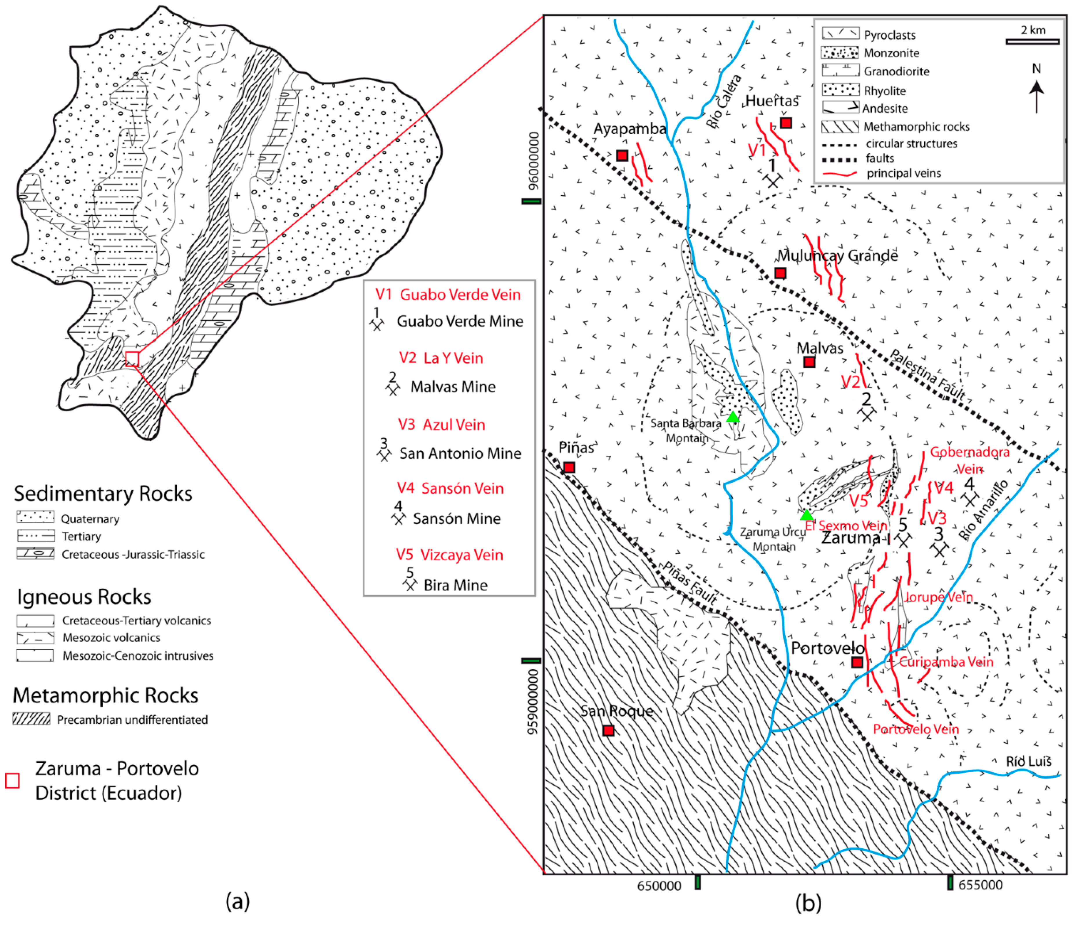
2. Geological Setting and Ore Mineralogy

The Zaruma-Portovelo epithermal deposits are in general associated with mantle derived calc-alkaline magmas fractionated at shallow levels inside rifted continental crust [36] related to Early Miocene continental arc magmatism. The Ecuadorian Western-South Cordillera (Figure 1a) principally comprises oceanic crust and oceanic island arc lithologies [37]. The basement rocks in this area consist of metamorphic rocks (Triassic). Above them, massive andesitic lavas are unconformably intruded by small plutons of diorite to granodiorite composition (Lower Cretaceous). Felsic volcanic lavas, pyroclastics and rhyolitic flows (Tertiary-Miocene) cap unconformably all of these units. This was followed by collapse and post-collapse rhyolitic activity, which generated most of the alteration and mineralization [38].
In the Zaruma-Portovelo area (Figure 1b), the epithermal vein-system is a result of hydrothermal processes close to a Miocene volcano that produced an andesitic to dacitic sequence. The identified ore and gangue mineral assemblages are typical for intermediate sulfidation epithermal gold vein deposits associated with Early Miocene continental arc magmatism [36,38,39,40,41], distinguishing three mineralization stages: quartz-pyrite, quartz-polymetallic and quartz-carbonate stages [36,38,39,40,41]. Three mineralized zones were defined by [31,41] for this deposit: (i) zone with pyritization (without gold) associated to stockworks and dikes close to Santa Barbara and Zaruma Urcu Mountains and vein selvages on the Portovelo-Zaruma axis; (ii) zone with predominant sulfides in gold-bearing quartz and quartz-adularia veins in the Portovelo-Zaruma axis and northeast of Santa Barbara Mountain area (La Y and Vizcaya veins); and (iii) zone with predominant sulfosalts and minor sulfides in gold-bearing quartz-calcite and quartz-chlorite veins around the central sulfide zone (Guabo Verde, Azul and Sansón veins). The main hydrothermal alterations types are propylitic, argillic, silicic and sericitic assemblages. Pyrite, chalcopyrite, sphalerite and galena are the dominant ore minerals and bornite, hematite, tetrahedrite, molybdenite and electrum are also present. Quartz and calcite are the most important gangue minerals.

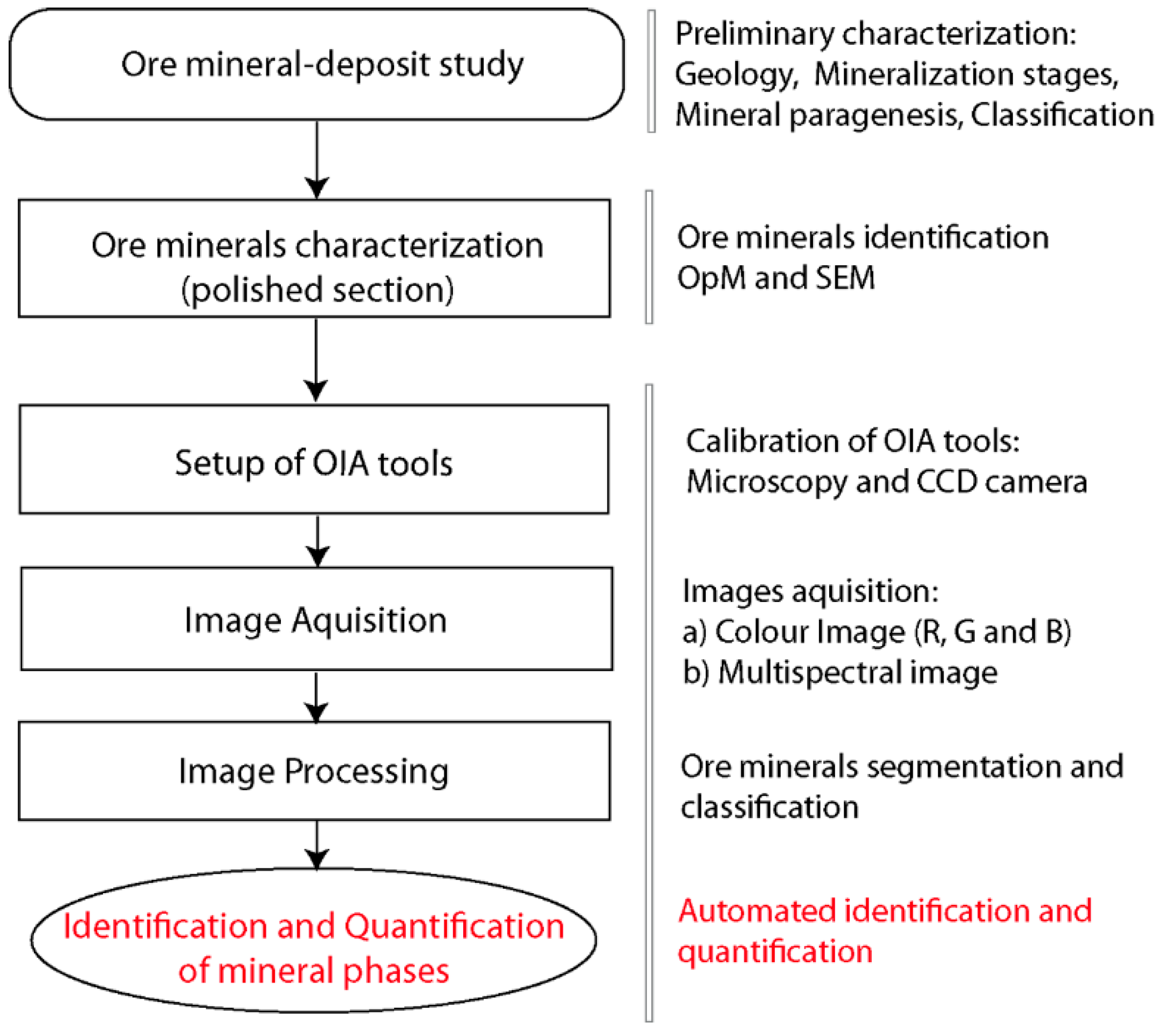
3. Materials and Methods

The procedure for the identification and quantification of mineral phases by OIA includes three main steps (Figure 2): the first step is the selection of representative samples and a visual ore mineral characterization yielding information about the site. The second step is the ore characterization comprising textural and mineralogical studies of the ore samples by OpM and SEM in polished sections, including a co-relation with preliminary studies. The final step is the OIA quantification of ore minerals found in polished samples (in Case 1, this means ore characterization using multispectral image analysis, and, in Case 2, gold characterization using RGB image analysis).

3.1. Sample Selection and Techniques

Samples from five sites (Figure 1b) were selected for the study, collecting 22 ore samples within the five ore veins: Sansón, La Y, Azul, Vizcaya and Guabo Verde (Table 1). These veins have significant economic mineralization (gold, silver and copper).
In order to study qualitatively the textural and mineralogical characteristics in ore samples (polished sections), optical microscopy (OpM) (Leica DM 6000 polarization microscope with magnification of 10× and 20×) and scanning electron microscopy (SEM) (JEOL 6100 SEM, using W-Filament, acceleration voltage of 20 kV and Inca Energy-200 software) were used (IGME, Oviedo). The identification of minerals in hand specimens (visual inspection with binocular microscope) and in the polished samples (study by OpM and SEM) represents a fundamental stage in implementing the quantification process by OIA. Automated identification and quantification by OIA will be conditioned by the mineral phases present and visible in the samples.
OIA is a technique designed for the automated identification and quantitative measurement of ore minerals based on their reflectance properties. In the present study, OIA was applied using an automated system developed by ETSIM Madrid based on multispectral reflectance values of ore minerals (Automated system for the identification and quantitative measurement of ore minerals -CAMEVA-), measured in visible, near IR and UV (375–1025 nm) light [24,32,43]. The system comprises a motorized reflected light microscope (Leica-DM-6000), a filter wheel (DTA RPF16) with 13 filters (Melles Griot: bandwidth 50 nm-FWHM-, between 375 nm and 1025 nm), a research B/W camera (BASLER SCA1400-17FM, interface IEEE-1394, an optical interface C-Mount 0.63×), an image analysis software (Aphelion 3.6) and, standard optical calibration (Ocean Optics STAN-SSH and STAN-SSL). Currently, 200 mineral images (20×) acquired for each polished section could be considered as representative for a sample in which the various ore species studied are abundant or ubiquitous [44]. In our study, we acquired 200 images (≈3.73·108 points per sample [9]) and will consider OIA measurements representative for major components (volume > 5%). However, statistical risk [45] increases significantly for minor components (1% < volume < 5%) and scarce species (volume < 1%). Therefore, a different strategy was applied for gold: not just a grid, but the whole surface of the section has also been analyzed, and then composed as a mosaic, so that not a single gold grain was missed.
RGB image analyses were conducted in the Oviedo IGME Laboratory. The imaging system used to capture color images is based on an RGB color model (i.e., in a RGB image of 24 bits, GL ranging in an 8-bit image from 0 to 255 for each R, G and B channel/band). RGB images are meant to show colored minerals as they are observed under the microscope. Color images were acquired using a ProgRes C5 (digital microscope camera with 5.0 Megapixel CCD-Color-2/3”, A/D conversion (max.) 3 × 8 Bit RGB, digital interface IEEE1394a firewire, optical interface C-Mount 0.63×) controlled by Image-Pro Plus-7.0 (image analysis software). According to [45], OIA quantification of visible gold (trace minerals and diameter >≈3 µm) in polished sections should be performed scanning the complete visible target mineral area. It is completed in order to get minimize error measuring all grains ore present in the samples with gold representative measurements. In our study, we will investigate the complete gold population visible in two samples. There exist some limitations to the OIA procedure related to the risk of misidentification caused by the spectral similarity of some ore minerals. Nevertheless, they could be reduced to a minimum if the ore deposit typology and the corresponding ore mineral species are defined previously [7].
OIA technique shows errors in quantification due to: (i) errors resulting from systematic observations of polished section (counting error); (ii) errors due to variability introduced by the user (operator error); or iii) errors encountered when 2D slices are used to estimate vol. % in the hand samples (specimen error). In our study, considering the quantification limited to polished section scale, specimen error is equivalent for OIA and microscopic estimation or point counting. In this study, we have not extrapolated measures in polished section to block samples or mineral deposit. Specimen error involves a sampling problem (sampling error). The errors due to counting-errors and operator-errors during quantification of mineralogical parameters were calculated based on methods of different authors [9,44,46,47]. In our case, the total error of the OIA (operator error) technique was 1.24% [47]. The counting error of OIA technique using 200 images by 20× magnification for mineralized area of 400 mm2 was about 1.95% [9,44]. Sampling error could be estimated using bootstrap resampling method [47]. In the case of gold measure by OIA, although all gold grains were acquired and quantified (about 300), for representative measures, more than 1000 particles will be required [46,47]. According to [11,48], OIA of polished sections comprises the following steps: setting up OIA tools, image acquisition, segmentation, feature extraction and classification. These stages of the present study are described below.

3.2. Setup of Equipment

According to [6,29,48], OIA is subjected to errors and the total error is accumulated at each individual step of sampling and analysis. The OIA tools of this study, which included a B/W camera, a color camera and an optical microscope, were updated before the image acquisition. A rigorous protocol for acquiring mineral images was established in order to warrant the reproducibility of method and results (Table 2). The following factors were considered for the evaluation and adjustment of OIA tools [6,11,32,48,49]: noise, spatial and temporal drifts, grey calibration, gain and geometric calibration. Image acquisition has to be done in optimal conditions including camera and microscope light source stabilization (Table 2).

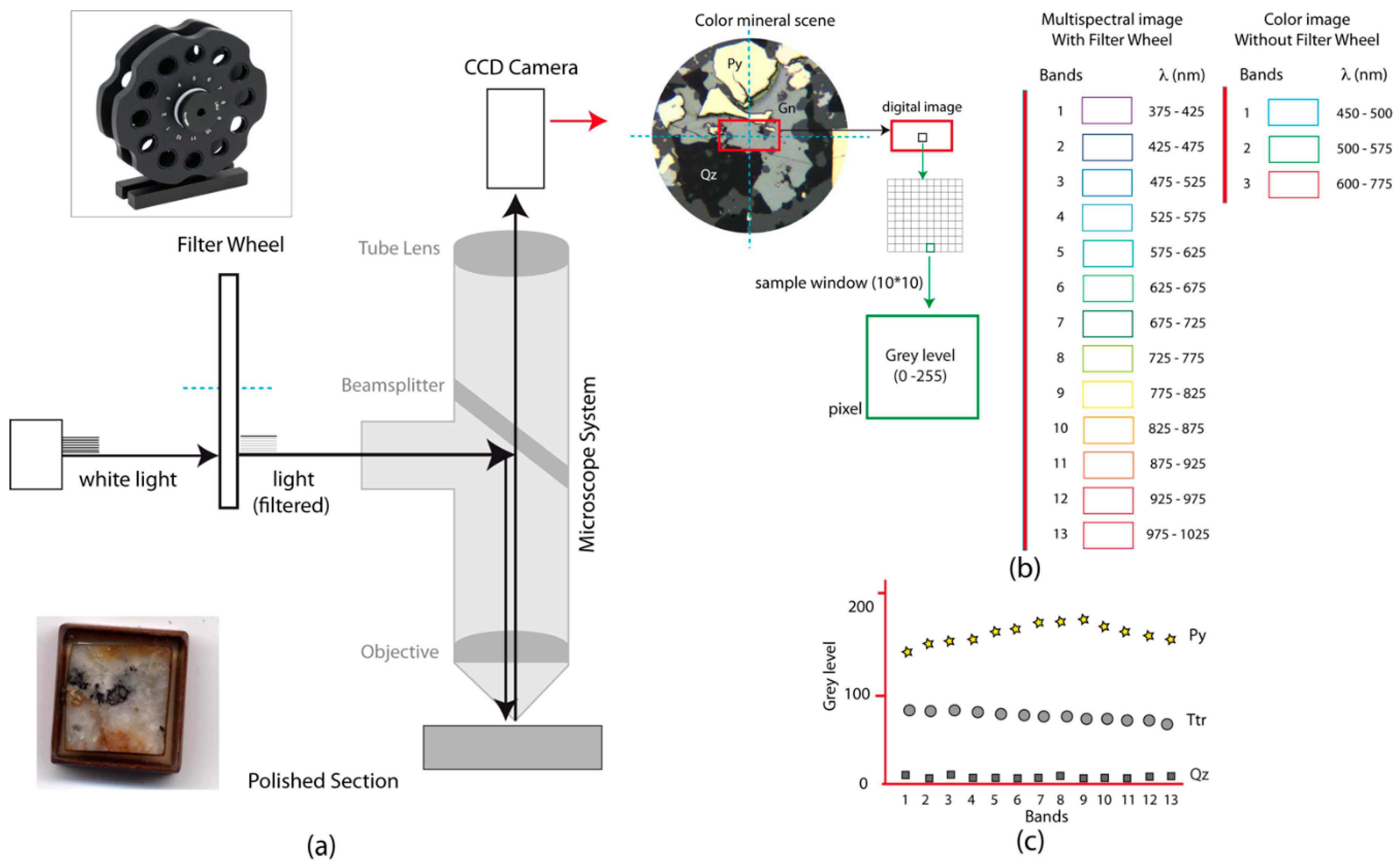
3.3. Image Acquisition

Multispectral images were acquired using the software of the B/W camera on the optical microscope (Figure 3a) with 13 wheel filters (CAMEVA System). A partial surface area (≈200 regions of interest by sample) of nine polished sections was studied. The procedure of image acquisition was as follows:
  • Selection of region of interest by manual focusing under non-polarized reflected light conditions. The ore samples were studied using objective lens 20× (N.A. 0.5). Total magnification was 460× (Table 2).
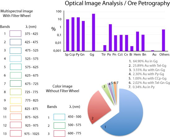
  • Automated establishment of the initial filter light conditions in the optical microscope. For each of the 13 filters an image of the same mineral scene is produced (noted as band 1 to 13). The image with the first filter corresponding to band 1 (375–425 nm bandwidth) is acquired (Figure 3b).
  • Time averaging: Eight images of the same scene with the first filter in a t-interval of 100 ms were acquired and averaged into a primary average image of band 1. This automated operation reduces electronic noise generated by the camera.
  • Saving the image in .tif format.
  • Automated movement of filter wheel to filter 2 (425–475 nm bandwidth), generating an image of band 2. This is followed by Steps 3 and 4 again. This operation was performed using all filters, producing 13 primary average images (Figure 3b).
  • Selection a new region of interest with automated (X-Y) displacements and focus (Z). The sequence is repeated until all regions of interest (≈200) are studied. Acquisition and quantification of 200 frames take about 4 h (each frame: 1.2 min).
RGB images were acquired using the software of the color camera on the optical microscope. The entire gold population of two polished sections was studied. The procedure was as follows:
7.
Selection of region of interest by manual focusing under non polarized reflected light conditions. The ore samples were studied using objective lens 20× (N.A. 0.5). Total magnification was 460× (Table 2).
8.
Time averaging: Images of the same scene in a t-interval of 100 ms were considered as a primary average image. This operation reduces electronic noise generated by the camera.
9.
Saving the image in .tif format.
10.
Automated separation of the color image into three channels: R, G and B.
11.
Selection a new region of interest with automated (X-Y) displacements and focus (Z). We repeated the sequence until all regions of interest (gold) were studied.

3.4. Image Segmentation

Image segmentation is the process of partitioning a digital image into multiple segments (sets of pixels) and it involves the identification and isolation of pixels that belong to a same category [51,52]. Ore mineral identification using image-processing techniques is usually achieved by segmentation based on edges or regions or a combination of both [6,21,32]. The segmentation ranges used for minerals segmentation were those established by [6,21] for color images and by [32,43,44] for multispectral images. The procedure was as follows:
  • Grey levels of each ore mineral in the polished section were calculated using a supervised training step. Sampling windows (10 × 10 pixels) were placed on regions that could be clearly considered as a specific ore mineral (mineral 1) in a primary average image (band 1). Normal distributions of grey levels were defined for the studied population.
  • For the mineral studied in band 1, mean (x) and standard deviation (σ) parameters were calculated. Segmentation ranges were defined as (x ± 3σ), with significance level of Y: 99.9%.
  • Saving the segmentation ranges for mineral 1 in band 1.
  • Selecting a new ore mineral (mineral 2) on an image in band 1 and repeating Steps 1 to 3 until covering all minerals (14 ore minerals + gangue) in this band.
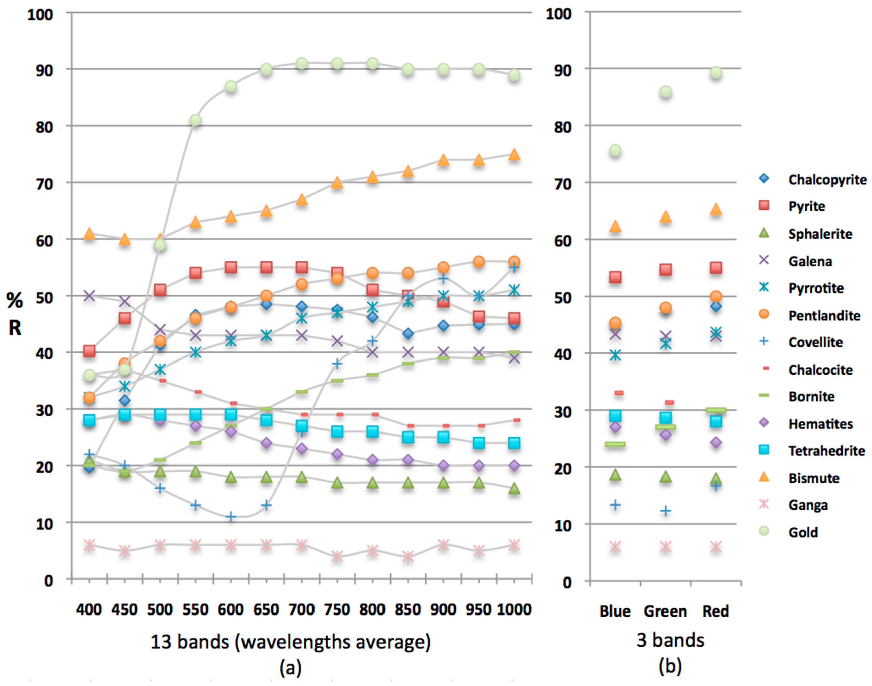
  • Selecting a new image (band 2) and repeating Steps 1 to 4. This operation is executed until all 13 bands or 3 bands are studied in multispectral image analysis or RGB image analysis, respectively.
Establishing segmentation ranges for all ore minerals in each spectral image [43,44], a final ore mineral segmentation is generated as the intersection of the 13 partial segmentations (applying minimum Mahalanobis distance classifier) [32]. Assuming a Gaussian distribution of grey levels (Y(μ − 3σ < X < μ+3σ): 99.7%), the final segmentation in multispectral image analysis had a level of Y: 98.7%. In RGB image analysis, final ore mineral segmentation is the intersection of three partial segmentations [6] with a level of Y: 99.1%. A simple check of the above segmentation ranges mentioned on our samples, following the same procedure was completed for local adjustments of segmentation ranges.

3.5. Feature Extraction

Once defined our objects (minerals), we selected the most appropriate mineral features for assessing their size and shape. The main parameters considered were the area (for all ore minerals), the diameter and the breadth (for gold particles). The area is measured as the sum of pixels having intensity values within the selected ranges. The diameter is measured as a line segment of a circle with similar area to the measured particle. The breadth is measured as minor distance between two tangential lines on the border of the object). Breadth concept has been used by metallurgical applications [21] for the improved analysis of particle size (gold grains). We have considered as gold particles mineral phases with sizes bigger than 4 pixels (ca. 0.40 µm2).

4. Results

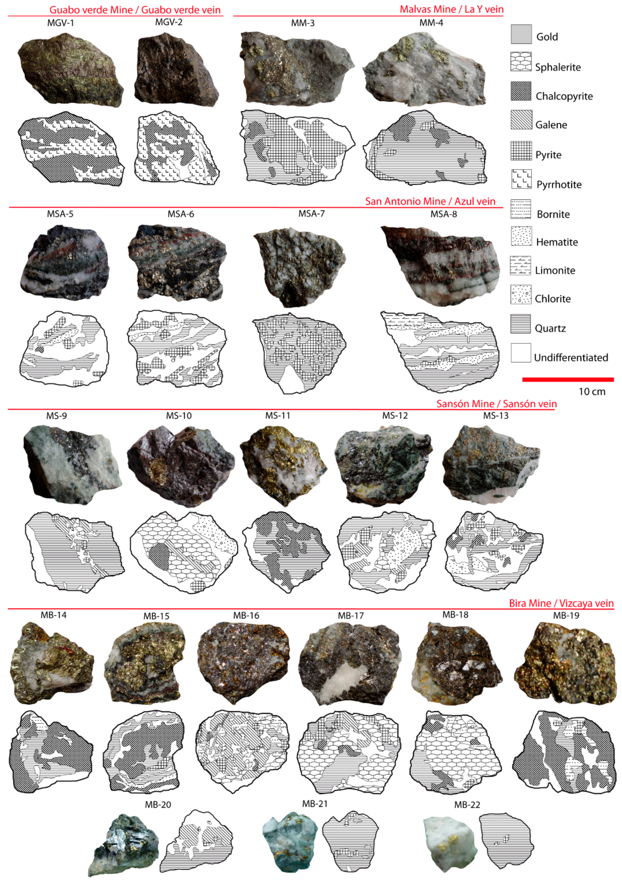
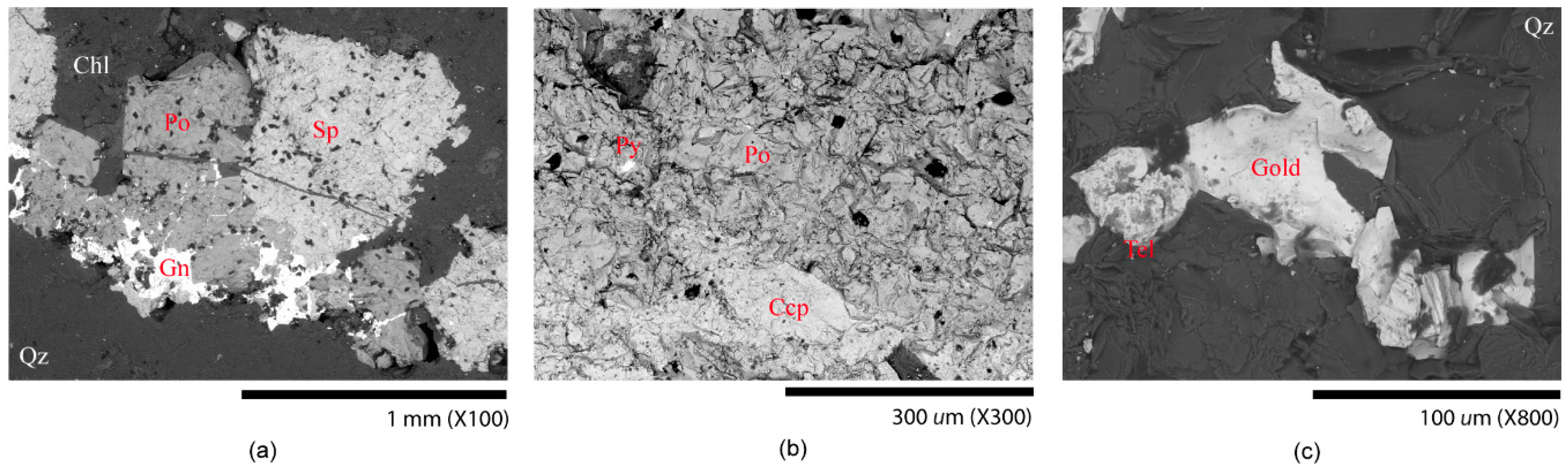
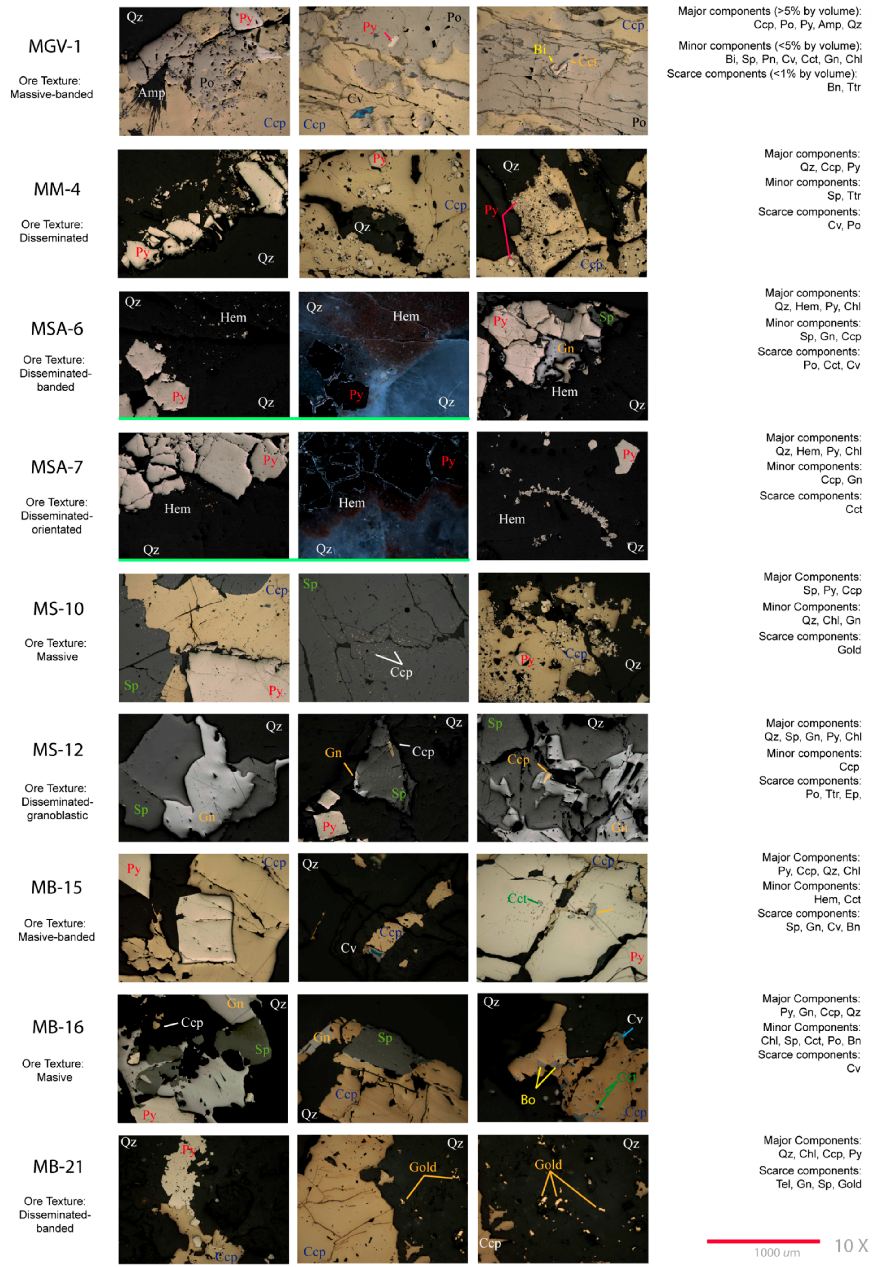
4.1. Microscopic Identification of Ore Minerals

Preliminary identification of minerals for each hand specimen (22 samples) is shown in Figure 4, in which the principal mineral species visible with unaided eye are shown. The mineralogy identified in the hand samples (gold, sphalerite, chalcopyrite, galena, pyrite, pyrrhotite, bornite, hematite, limonite, chlorite and quartz) and their description (i.e., MSA 5-6-8, banded quartz-pyrite-chlorite vein with pyrite-galena-sphalerite) allowed to: (i) corroborate that samples collected have representative mineralogy of the deposit; and (ii) choice samples to make polished sections. The results of the detailed microscopic study are shown in Figure 5, which displays representative mineral images, the main ore minerals and the ore texture, for each studied sample.
The study by reflection microscope and SEM permitted the identification of 13 ore minerals: gold, sphalerite, chalcopyrite, galena, pyrite, pyrrhotite, bornite, hematite, chalcocite, pentlandite, covellite, tetrahedrite and native bismuth. Furthermore, four gangue minerals were identified: quartz, amphibole, chlorite and epidote. In general, the textures correspond to a hydrothermal infill mainly characterized by open space filling textures (e.g., crustification, comb structure and symmetrical banding) and combined effects of local replacement and open space filling. The gold bearing samples (e.g., MB-21 in Figure 5) were identified as a quartz and sulfide ore with partially brecciated vein filling texture. Major components are quartz, chlorite, chalcopyrite and pyrite, minor components are galena and sphalerite and accessory components are gold and tellurides. The dominant mineral association is quartz-chlorite that forms coarse-grained crystalline aggregates. The sulfide phases are scattered or associated with quartz crystal aggregates. The identified mineral assemblages and textures are consistent with those of a hydrothermal filling (massive, massive-banded, disseminated-oriented and disseminated), already defined in previous research, and referred to as intermediate sulfidation epithermal deposit [36].
Complementary SEM studies were performed in specific samples (MGV-1, MS-12 and MB-21), sustaining descriptions made with the optical microscope about mineralogy, textures and gold mineralogical associations (Figure 6).

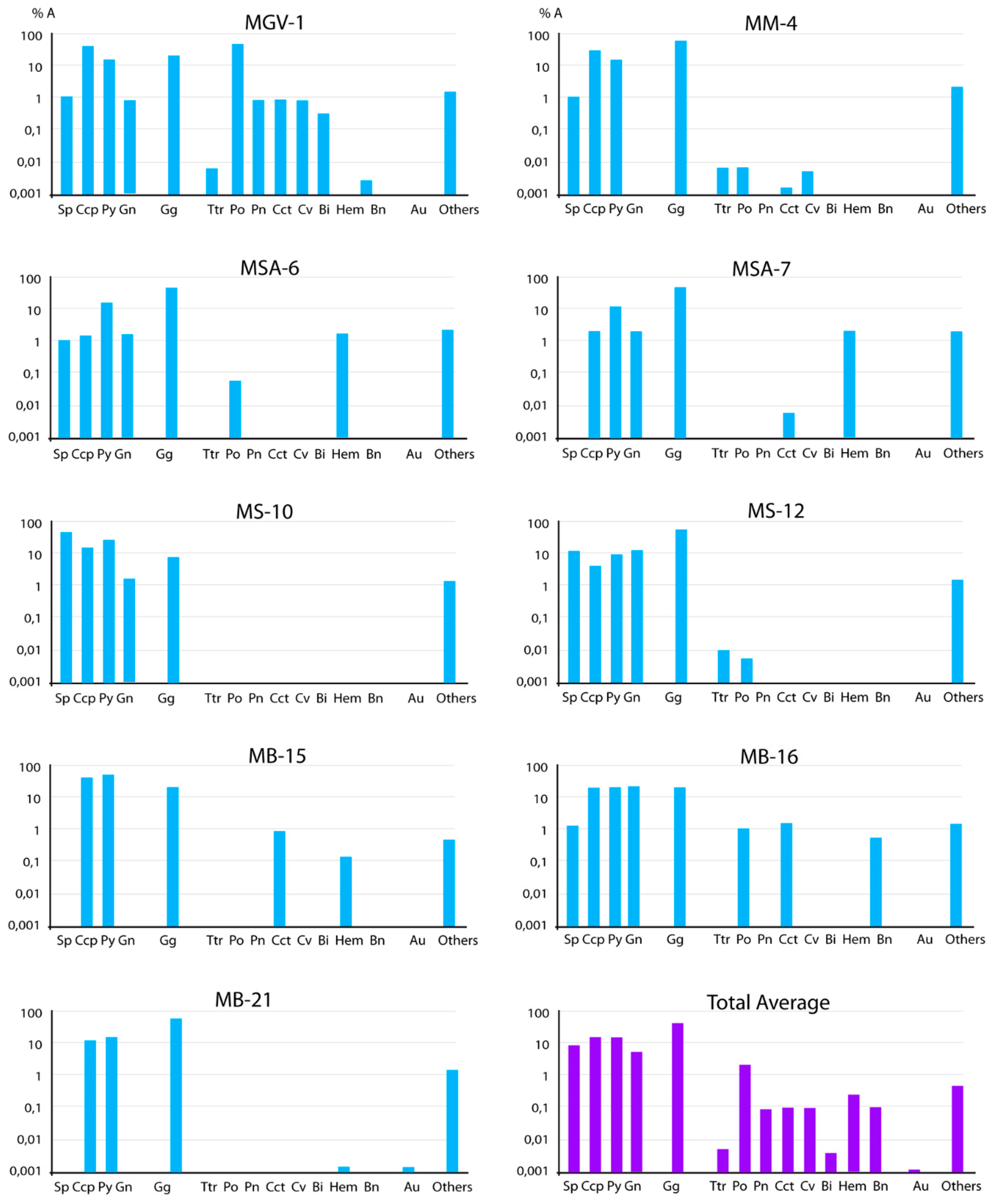
4.2. Ore Characterization by OIA (Case I)

The identification and quantification of opaque minerals by OIA was carried out in nine polished sections. The measurement process by CAMEVA multispectral analysis system was applied on mineral images acquired with a 20× magnification. The acquired images comprised 200 scenes of the mineral surface of each of the selected polished sections. The CAMEVA system allows the user to start the quantification process indicating the type of mineral deposit to study and then selecting the identified mineralogy from a theoretical ore mineralogical database [43]. This was because the local check of segmentation ranges completed in our samples did not generate any important change. The system also permits manual selection of minerals previously identified in each sample. The 13 ore minerals cited above (Section 4.1) were also checked and successfully identified by the automated CAMEVA system by means of their VNIR (visible and near-infrared) spectra.
The area of detected mineral grains is depicted in diagrams plotting the relative area of minerals of each mineral phase (Figure 7). An automated search provides data on the occurrence and distribution of the selected ore mineral grains. The quantified average abundance (% area) of minerals indicated the presence of four major sulfides: chalcopyrite (12%), pyrite (10%), sphalerite (9%) and galena (6%). Eight scarce mineral phases (between 0.001% and 1% each), 60% of gangue (quartz, chlorite and calcite), 0.0001% of gold and 2% of unidentified minerals, were also measured.

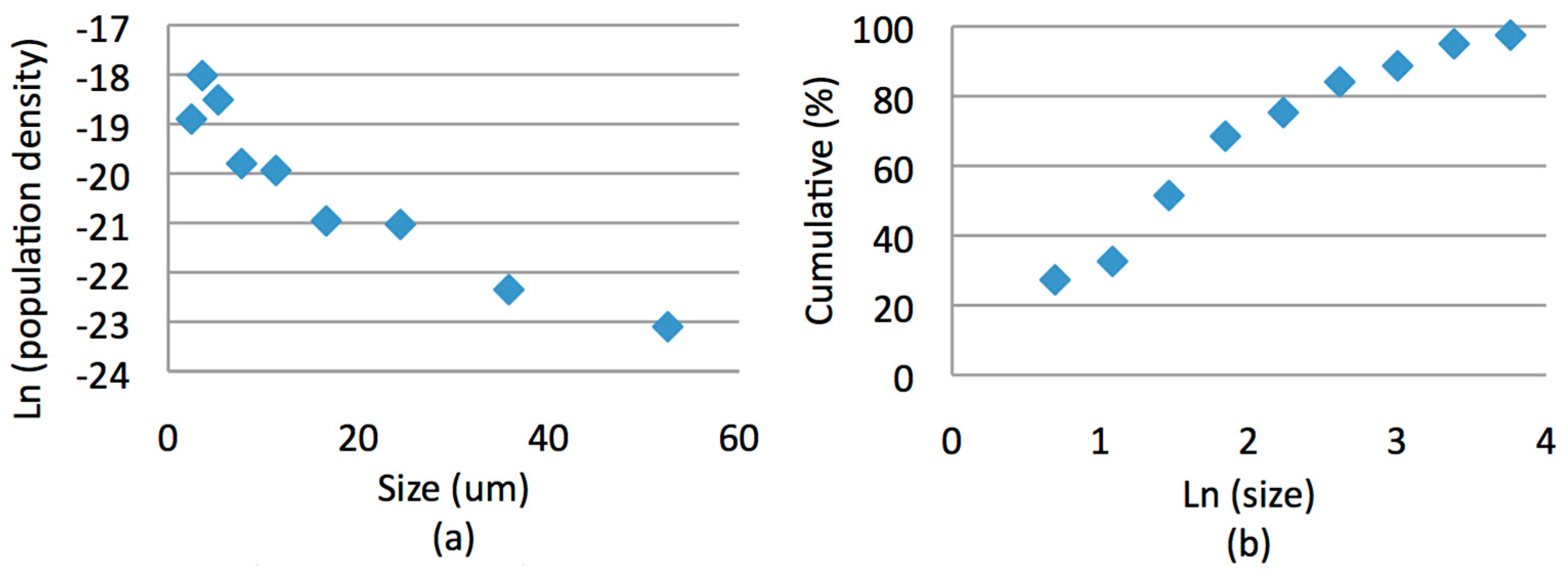
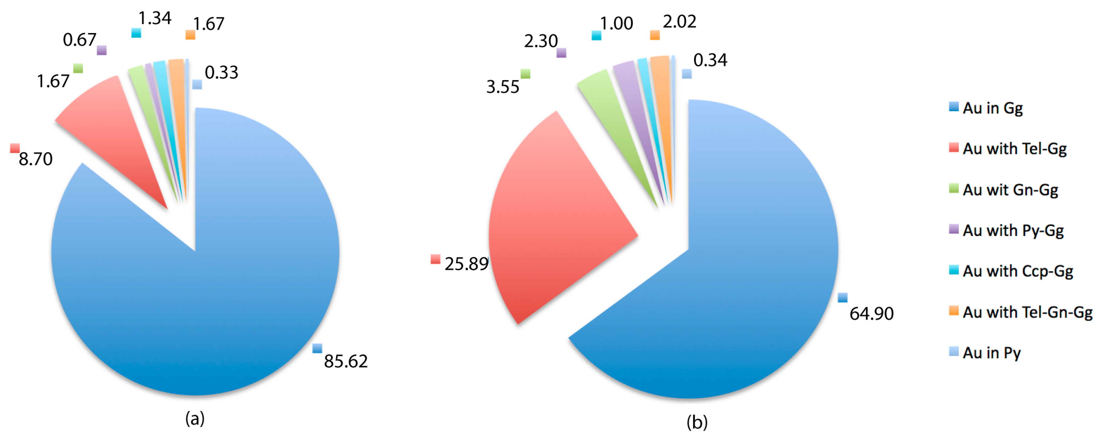
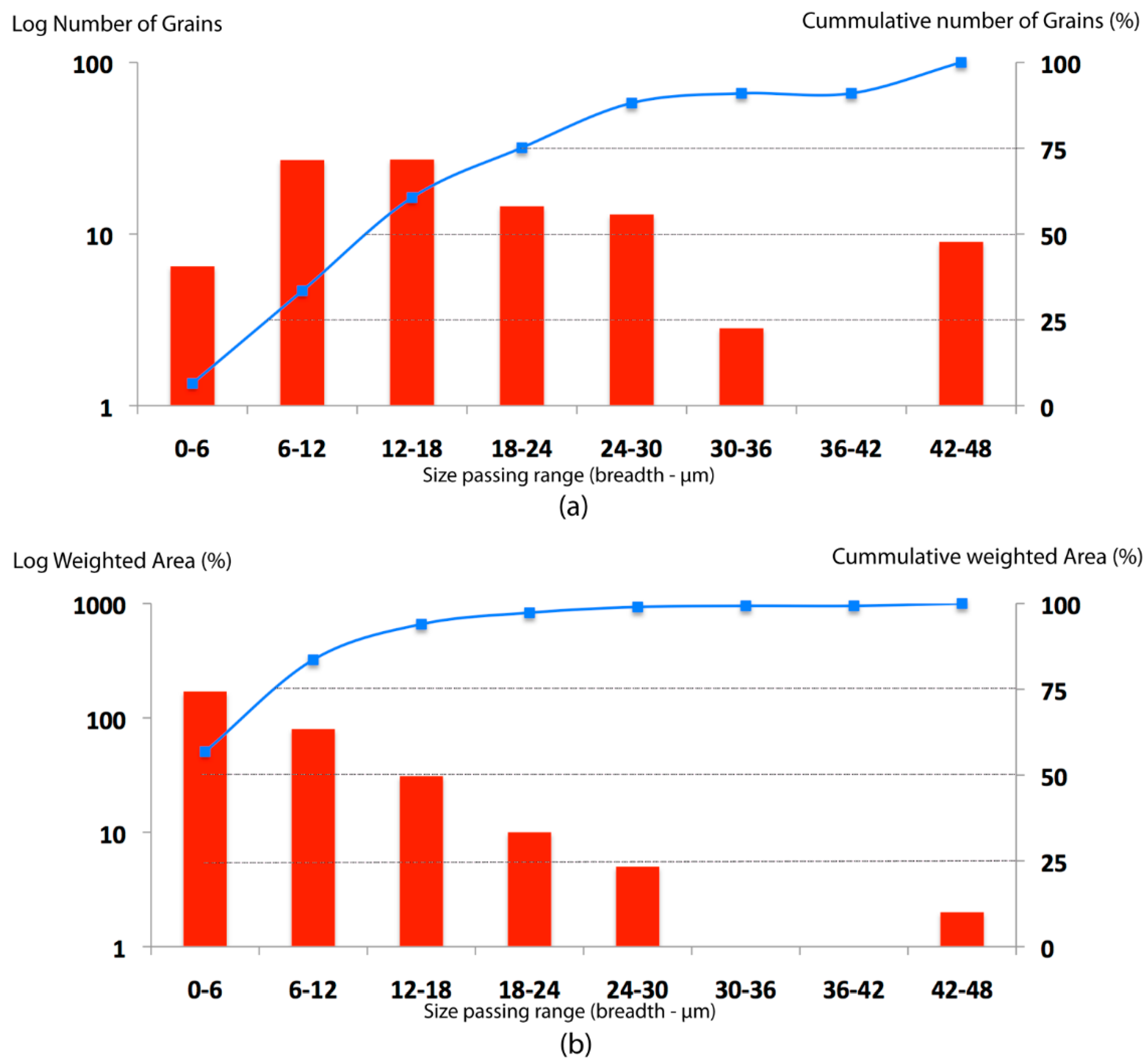
4.3. Gold Characterization by OIA (Case II)

The detailed quantification of gold by OIA was developed on specimens where previous mineralogical studies determined the presence of this mineral phase in significant quantities (approximately 300 gold grains on 8 cm2 studied area). The samples MB-21 and MB-21b, chosen for this study, correspond to the Vizcaya vein. The quantified gold (native gold and/or gold with variable silver and electrum contents) has appropriate particle sizes for observation by optical microscope with a magnification of 20×. The measurement process was performed using color analysis with the system of IGME-Oviedo and following a specific OIA protocol. Segmentation ranges used for gold segmentation were R: 220 ± 35, G: 205 ± 40 and B: 110 ± 45. Gold quantification (area, diameter and breadth) of the two specimens gave the following results: The gold area in the polished samples (27,198 μm2) is approximately 0.0034% of the total area of the ore minerals (8 cm2). The number of gold grains identified and quantified is 299. The area of the individual gold grains range is between ca. 0.40 and 1300 μm2. The statistical analysis of the area of gold grains shows an average of 90.97 μm2, a median of 26.67 μm2 and a standard deviation of 162.22 μm2. On the other hand, the range of gold grain breadth is between ca. 0.31 and 46.20 µm, with an average of 6.88 µm, a mean of 5.02 µm and a standard deviation of 6.71 µm. The range of gold grain diameter is between ca. 0.70 and 40.60 µm, with an average of 7.92 µm, a mean of 5.83 µm and a standard deviation of 7.30 µm.
OIA made it possible to quantify the distribution of gold particles (frequency and area) by the mineral association (included or in contact with gangue or sulfides). A gold grain that is completely surrounded by another mineral (i.e., included) is referred to by the word “in”. A gold grain positioned on the edge of another mineral (i.e., in contact with) is referred to by the word “with”.
The gold grains are mostly included in quartz but also in contact and/or included in sulfides. Detailed results are presented in Figure 8. It was also possible to classify these associations by the size passing range (particle breadth). Eight interval classes (breadth range in µm and class intervals: 6 µm) were established to describe the distribution of the data. These data are shown in Table 3 and Table 4.
Gold is found mostly as free gold or gold in gangue (64.90% of the area of gold and the 85.62% of the gold grains). This mineral association was identified automatically by the OIA system. The other associations, however, were checked manually on a grain by grain basis due to small grain size and related segmentation problems in mineral interfaces (contacts). Once completed the operator’s survey, the measurements of area and breadth were again carried out automatically by the software. Thus, 34,76% of the gold area related to the 14.04% of the gold grains corresponds to gold in partial contact with gangue and some other mineral phase like pyrite, galena, chalcopyrite or tellurides (hessite). Finally, 0.34% of the gold area related to the 0.33% of the gold grains corresponds to gold completely included in pyrite. Absolute and relative (cumulative) curves of number of gold grains (Figure 9a) and of gold weighted area (Figure 9b) versus breath range (in µm and class intervals: 6 µm) distribution were plotted. Data distribution shows the following breadth values of the gold grains for the main percentiles: 2.05 µm (Q25); 5.10 µm (Q50) and 9.96 µm (Q75) for number of grains and 10.26 µm (Q25); 15.53 µm (Q50) and 22.15 µm (Q75) for weighted area. The accumulated gold grain areas corresponding to these percentiles are: 667 μm2 (Q25), 1341 μm2 (Q50) and 1990 μm2 (Q75). Frequency diagram of number of gold-grains related to gold size passing classes (breadth, µm) and diagrams of weighted gold-grain area related to gold size passing classes (breadth, µm) in Figure 9 suggest a log normal size distribution although, the presence of gold grains (Figure 9b) with large size passing range (42–48 microns) would not correspond with the log normal distribution.
According to [53], the stereology of conversion of two-dimensional data obtained from study of polished sections is complex but can be approximated for convex shapes. Crystal size distribution (CSD) correction [53] could be applied on actual size distribution (2D-3D) with program CSD Corrections 1.52 [54]. Particle size measurements (e.g., diameter) are obtained from the binary images of gold grain and converted in 3D size distribution by correcting data by means of the Schwartz–Saltikov method [53]. An example of CSD diagrams calculated for gold grains measured by OIA are shown in Figure 10. These diagrams have allowed to optimize statistics for the largest grains (less abundant) and to reveal the details of the smallest grains distribution. For all gold grains, a linear correlation ln N(L) vs. size (L) diagrams is evidenced, supporting the gold CSD scale invariance over sizes ranging from about 0.1 up to more than 65 µm.

5. Discussion

5.1. OIA System

OIA as a mineralogical quantification tool presents an important advance in ore characterization and predictive metallurgy [16,17]. As has been shown in previous research, automated quantification of mineral phases by digital techniques [6,9,22,25,32,55] is appropriate for systematical and automatic mineral quantification in polished sections. Our results of the mineral abundance measurement (A%, Figure 9) give an example of the contribution that the OIA technique can make to qualitative mineragraphic descriptions.
According to [17,29], multispectral image analysis has demonstrated its superior potential with respect to conventional color imaging. A complete set of filters permits: (i) obtaining information even out of the visible region (Figure 11a), thus expanding the range of analysis; and (ii) obtaining a stack of multispectral images that can be segmented using multivariate discrimination. Thus, multispectral imaging yields additional information as compared to color imaging mode [29]. However, using RGB images, difficulties remain when opaque minerals have similar colors and reflectivity (Figure 11b and Table 5) in plane light, making it virtually impossible to distinguish them [17]. Some ore minerals studied here show overlapping characteristics (grey intensity values or reflectance) under the white light of the color camera. Some examples of common overlapping minerals found in our samples are: covellite-sphalerite-hematite-tetrahedrite-chalcocite (Reflection: 17%–30%) and pyrrhotite-galena-chalcopyrite-pentlandite (Reflection: 41%–48%). In Figure 11b, it is possible to see the overlapping of minerals (average of Reflection -%-). The application of the multispectral CAMEVA System, using wavelength specific filters allowed overlapping minerals to be separated (Figure 11a and Table 5).
RGB image analysis could be considered a simplification of a multivariate system where reflectance spectrum is limited to the visible spectrum in three bands (red, green and blue). According to [17,56], using RGB camera, the differences in these two parameters (reflectance and color) of opaque minerals are often great enough to make a clear distinction, especially in simple mineral assemblages. In our study, gold reflectance intensity and spectra were easily distinguished when comparing them to other minerals in the studied polished sections (Figure 10b). The quantification of the gold area and breadth (Figure 8 and Figure 9) yielded a detailed characterization of the abundance and geometry of this mineral in our samples, thus contributing important geometallurgical information, e.g., to optimize milling, ore recovery and processing method.
The present research sought to optimize the benefits of each of these applications. Thus, multispectral discrimination analysis was applied to identify and quantify various mineral phases (mineralogical abundance for every mineral in each studied polished section), while RGB analysis focused on the study of gold (geometric characterization and mineral association). In this study, OIA quantification must be considered representative on the polished section scale. Numerical support contributed by OIA is complementary to qualitative ore petrographic studies, and provides an essential tool to optimize geometallurgical processes. Its reliable application to assess industrial problems implies always, as a previous necessary requirement, a careful sampling and preparation procedure, ensuring that the sections are statistically representative of the orebody. The representativeness of the polished section in relation to the whole ore deposit, which must never be neglected, is however out of the scope of this contribution.
Despite the limitations of OIA due to difficult identification of mineral phases with similar reflectance and color and the impossibility to measure chemistry, the quantification method using digital images (multispectral and/or color) represents an accessible and relatively inexpensive option compared to new mineral quantification systems like QEMSCAN and MLA [13,57]. The use of integrated microscopes with image analysis systems allows the user to obtain a robust analysis, flexibility in the operating mode and speed of operation where more costly and complicated techniques are impractical. However, we must emphasize the importance of an expert operator to control and monitor the automatic OIA processes. This applies as well for SEM-based systems. According to [57,58], a combined approach using OIA techniques and new mineral quantification systems (e.g., QEMSCAN) will provide the most detailed understanding of ore mineral samples characterized.
It is important to comment that measures by OIA on multispectral images using 200 frames at 20× magnification (about 25 mm2) of the polished section (about 400 mm2) are conditioned by specimen error, counting error and operator error [9,44,46,47]. To polished section scale, counting error could be reduced studying totally mineralized area, in this case, measurement would last 45–60 h instead of 3–4 h. Nevertheless, the results obtained by the application of multispectral analysis in 200 frames per sample allowed a preliminary quantification of the abundance of each mineral in the samples selected. This served as a guide to plan more detailed analysis (i.e., quantification of gold measuring all grains present in the samples where it was identified). For detailed grain size distribution analysis, it is necessary to confirm the area of particle sections, which needs to be measured to achieve the required level of error in measured textural data (sampling error). This could be possible applying bootstrap resampling technique [47]. In the case of gold, about 300 grains were identified and quantified in two polished sections using OIA on color images with satisfactory results. The measurements made by OIA in this article were not focused on the characterization of the mineral deposit from which the samples were obtained. The work aims to be a complement to ore-petrographic studies and its precision at polished section scale. This will be subject to operator error and to the quantity of scattered frames over the entire surface of the specimen mineralized.

5.2. OIA Measures

The study of the samples from Zaruma-Portovelo mineral deposit (Figure 1a) by optical microscopic and optical image analyses has allowed corroborating information about vein mineralizations in two of three zones defined by [31,41] for this deposit: (a) zone with predominant sulfides in gold-bearing quartz and quartz-adularia veins in the Portovelo-Zaruma axis and northeast of Santa Barbara Mountain area (La Y and Vizcaya veins); and (b) zone with predominant sulfosalts and minor sulfides in gold-bearing quartz-calcite and quartz-chlorite veins around the central sulfide zone (Guabo Verde, Azul and Sansón veins). In our samples studied, the two types of mineralization associated with gold (sulfide and sulfosalts zones) are found and quantified in the same sample, highlighting overlapping alteration phases [41].
Furthermore, regarding the three successive mineralization stages distinguished by [41,42] in the mineral deposit studied: (i) quartz-pyrite stage (quartz-pyrite-chlorite-hematite; quartz-pyrite-chalcopyrite parageneses); (ii) quartz-polymetallic stage (quartz-galena-sphalerite; galena-chalcopyrite; sphalerite-pyrite-chalcopyrite-tetrahedrite-telluride-gold parageneses); and (iii) quartz-carbonate stage (quartz-calcite-pyrite parageneses). Our study, in addition to identifying the parageneses indicated above, has allowed the identification of other minerals such as pyrrhotite, bismuth native, chalcocite, pentlandite and bornite, also mentioned by [41].
In relation to visible gold identified in the samples from Vizcaya vein where, its mineral assemblage, abundance and relation between grain size and mineral association was quantified (Figure 8, Table 3 and Table 4), a better characterization of the mineralization stage in Zaruma-Portovelo mineral deposit (quartz-polymetallic stage) has been provided. The modal analysis obtained by OIA shows that the main minerals in contact with the gold are gangue and tellurides, there are also small amounts of chalcopyrite, galena and pyrite. A small proportion of the gold grains (0.34%) are included in pyrite, implying few difficulties to gold liberation.

6. Conclusions

The Zaruma-Portovelo mineral deposit study has provided a good test for the OIA methodology, allowing to corroborate previous characterizations of this ore deposit and to add more information about it (petrography and geometallurgy). From the methodological point of view, quantifying ores by OIA is feasible provided the following conditions are fulfilled:
  • The application, as well for optical as for SEM-based systems, should be supervised by an expert, and not be understood as a blackbox. A prior qualitative description of the mineralogy and information about the mineral deposit from which the ore samples come from may be welcome inputs, since the introduction of these mineralogical and metallogenetic criteria in the process of automated identification of mineral phases may avoid confusion in the recognition of mineral phases with equivalent GL response.
  • Equipment set-up ensuring optimum acquisition of images. Control of physical and electronic factors (polishing quality, stability-intensity light source, noise removal, etc.) during image acquisition limits the GL variation in the mineral phases, facilitating proper identification.
  • A preliminary study of GL responses (R, G and B bands in the color image and 13 bands in multispectral image) of the identified mineral phases to check ore identities with segmentation ranges defined in the literature, or available at [6,43]. The application of segmentation ranges for minerals of interest is performed for each of the distinct bands composing the images (color/multispectral), guaranteeing a correct classification.
  • The OIA systematic described in this paper can be applied in the study of other mineral deposits in the world. OIA could be used to provide initial ore mineral quantification at polished section scale with relatively low economic investment. It is a simple and accessible method that ensures the reproducibility of measurements and processes by following clearly defined protocols.
Regarding the results of the two case studies, RGB and multispectral analysis of samples of five veins of Zaruma-Portovelo yielded the following outcomes:
  • Automated identification and quantification of 15 mineral phases using multispectral images (Case 1) was carried out. These phases were previously identified with reflected light optical microscopy and by visual inspection with a binocular microscope, and they agreed with the expectations based on previous studies. The results of this experiment show that the ore mineral quantification on polished sections is possible applying OIA methods, allowing obtaining complementary information to traditional (qualitative) ore petrographic studies.
  • Detailed characterization of gold present in two of the polished samples (Case 2) was carried out using RGB images. Color images were acquired with 20× magnification of all the grains of gold present (299). These quantifications may provide an important contribution to more detailed studies focused on geometallurgical optimization through measurements of mineral associations, mineral liberation grade, mineral grain size and distribution and textural data.

Acknowledgments

The authors would like to express their thanks for the funding of this work provided through the Minería XXI Project (CYTED: 310RT0402). We also thank Xavier Valverde, Pablo López, Flavio Romero and Oscar Emilio Loor for their help and the authorization for rock sample collection in Gold Mines, Zaruma and Timea Kovacs for her suggestions. We also would like to thank the editorial office for the editorial handling and three anonymous reviewers for their constructive comments and corrections.

Author Contributions

Wilson Bonilla, Richard Banda, Paúl Carrion and Stallin Puglla collected the ore samples, studied hand samples and completed the geological setting of ore mineral deposit studied; Edgar Berrezueta, Berta Ordóñez-Casado and Ricardo Castroviejo conceived, designed and performed the experiments by Optical microscopy, SEM and optical image analysis; Edgar Berrezueta, Berta Ordóñez-Casado and Ricardo Castroviejo contributed analysis tools and analyzed the data of OIA measures; Edgar Berrezueta, Berta Ordóñez-Casado, Ricardo Castroviejo and Wilson Bonilla wrote the paper; and all authors participated in discussion and conclusion of this research article.

Conflicts of Interest

The authors declare no conflict of interest.

Abbreviations

The following abbreviations are used in this manuscript:
Ampamphibole
Augold
Bibismuth native
Gngalena
Augold
Hemhematite
Bibismuth native
Lmlimonite
Bnbornite
Pypyrite
Ccpchalcopyrite
Pnpentlandite
Cctchalcocite
Popyrrhotite
Chlchlorite
Spsphalerite
Cvcovellite
Teltellurides
Epepidote
Ttrtetrahedrite
Gggangue
Qzquartz (Whitney and Evans, 2010)
OIAOptical Image Analysis
MLAMineral liberation analyzer
QEMSCANQuantitative evaluation of minerals by scanning electron microscopy
CCDCharge-coupled device
GLGrey levels
RGBRed, green and blue system
B/WBlack and white
OpMOptical microscopy
SEMScanning electron microscopy
ETSIMEscuela Superior de Ingenieros de Minas
IGMEInstituto Geológico y Minero de España
IRInfrared
UVUltraViolet
CAMEVAAutomated system for the identification and quantitative measurement of ore minerals
VNIRThe visible and near-infrared
CSDCrystal size distribution

References

  1. Agarwal, J.C.; Schapiro, N.; Mallio, M.J. Process petrography and ore deposits. Min. Congr. J. 1976, 62, 28–35. [Google Scholar]
  2. Amstutz, G.C. How microscopy can increase recovery in your milling circuit. Min. World 1962, 24, 19–23. [Google Scholar]
  3. Schwartz, G.M. Solving metallurgical problems with the reflecting microscope. Eng. Min. J. 1923, 116, 237–238. [Google Scholar]
  4. Craig, J.; Vaughan, D. Ore Microscopy & Ore Petrography, 1st ed.; John Wiley and Sons. Inc.: New York, NY, USA, 1981; p. 406. [Google Scholar]
  5. Poliakov, A.; Donskoi, E. Automated relief-based discrimination of non-opaque minerals in optical image analysis. Miner. Eng. 2013, 55, 111–124. [Google Scholar] [CrossRef]
  6. Berrezueta, E.; Castroviejo, R. Automated microscopic characterization of metallic ores with image analysis: A key to improve ore processing. I: Test of the methodology. Rev. Metal. 2007, 43, 294–309. [Google Scholar] [CrossRef] [Green Version]
  7. Castroviejo, R.; Berrezueta, E. Automated microscopic characterization of metallic ores with image analysis: A key to improve ore processing. II. Metallogenetic discriminating criteria. Rev. Metal. 2009, 45, 439–456. [Google Scholar] [CrossRef] [Green Version]
  8. Ehrlich, R.; Kennedy, S.K.; Crabtree, S.J.; Cannon, R.L. Petrographic image analysis: Analysis of reservoir pore complexes. J. Sediment. Petrol. 1984, 54, 1365–1378. [Google Scholar]
  9. Grove, C.; Jerram, D.A. jPOR: An ImageJ macro to quantify total optical porosity from blue-stained thin sections. Comput. Geosci. 2011, 37, 1850–1859. [Google Scholar] [CrossRef]
  10. Russ, J.C. Computer Assisted Microscopy the Measurement and Analysis of Images, 1st ed.; Plenum Press: New York, NY, USA, 1990; p. 453. [Google Scholar]
  11. Pirard, E.; Lebrun, V.; Nivart, J.F. Optimal image acquisition of video images of reflected light. Eur. Microsc. Anal. 1999, 60, 9–11. [Google Scholar]
  12. Reedy, C.L. Review of digital image analysis of petrographic thin sections in conservation research. J. Am. Inst. Conserv. 2006, 45, 127–146. [Google Scholar] [CrossRef]
  13. Anderson, K.F.E.; Wall, F.; Rollinson, G.K.; Moon, C.J. Quantitative mineralogical and chemical assessment of the Nkout iron ore deposit, Southern Cameroon. Ore Geol. 2014, 62, 25–39. [Google Scholar] [CrossRef]
  14. Rollinson, G.K.; Andersen, J.C.O.; Stickland, R.J.; Boni, M.; Fairhurst, R. Characterisation of non-sulphide zinc deposits using QEMSCAN®. Miner. Eng. 2011, 24, 778–787. [Google Scholar] [CrossRef]
  15. Santoro, L.; Boni, M.; Rollinston, G.K.; Mondillo, G.; Balassone, G.; Clegg, A.M. Mineralogical characterization of the Hakkari nonsulfide Zn(Pb) deposit (Turkey): The benefits of QEMSCAN®. Miner. Eng. 2014, 69, 29–39. [Google Scholar] [CrossRef]
  16. Donskoi, E.; Suthers, S.P.; Fradd, S.B.; Young, J.M.; Campbell, J.J.; Raynlyn, T.D.; Clout, J.M.F. Utilization of optical image analysis and automatic texture classification for iron ore particle characterisation. Miner. Eng. 2007, 20, 461–471. [Google Scholar] [CrossRef]
  17. Lane, G.R.; Martin, C.; Pirard, E. Techniques and applications for predictive metallurgy and ore characterization using optical image analysis. Miner. Eng. 2008, 21, 568–577. [Google Scholar] [CrossRef]
  18. Spring, K.R. Cameras for digital microscopy. Methods Cell Biol. 2007, 81, 171–186. [Google Scholar] [PubMed]
  19. Köse, C.; Alp, I.; Ikibas, C. Statistical methods for segmentation and quantification of minerals in ore microscopy. Miner. Eng. 2012, 30, 19–32. [Google Scholar] [CrossRef]
  20. Berrezueta, E.; Castroviejo, R.; Pantoja, F.; Álvarez, R. Mineralogical study and digital image analysis quantification of gold ores from Nariño (Colombia). Application to the improvement of the ore processing. Bol. Geol. Min. 2002, 113, 369–379. [Google Scholar]
  21. Castroviejo, R.; Berrezueta, E.; Lastra, R. Microscopic digital image analyses of gold ores. A critical test of the methodology, comparing Reflected Light and SEM. Miner. Metall. Process. 2002, 19, 102–109. [Google Scholar]
  22. Goodall, W.R.; Scales, P.J. An overview of the advantages and disadvantages of the determination of gold mineralogy by automated mineralogy. Miner. Eng. 2007, 20, 506–517. [Google Scholar] [CrossRef]
  23. Petersen, K.R.P.; Aldrich, C.; Van Deventer, J.S.J. Analysis of ore particles based on textural pattern recognition. Miner. Eng. 1998, 11, 959–977. [Google Scholar] [CrossRef]
  24. Castroviejo, R.; Brea, C.; Pérez-Barnuevo, L.; Catalina, J.C.; Segundo, F.; Bernhard, H.J.; Pirard, E. Using computer vision for microscopic identification of ores with reflected light: Preliminary results. In Proceedings of the 10th biennial SGA Meeting, Smart Science for exploration and Mining, Townsville, Australia, 17–20 August 2009; pp. 682–684.
  25. Delbem, I.D.; Galéry, R.; Brandão, P.R.G.; Peres, A.E.C. Semi-automated iron ore characterisation based on optical microscope analysis: Quartz/resin classification. Miner. Eng. 2015, 82, 2–13. [Google Scholar] [CrossRef]
  26. Bartolacci, G.; Pelletier, P.; Tessier, J.; Duchesne, C.; Bosse, P.A.; Fournier, J. Application of numerical image analysis to process diagnosis and physical parameter measurement in mineral processes-Part I: Flotation control base on froth textural characteristics. Miner. Eng. 2006, 19, 734–747. [Google Scholar] [CrossRef]
  27. Pérez-Barnuevo, L.; Pirard, E.; Castroviejo, R. Textural descriptors for multiphasic ore particles. Image Anal. Stereol. 2012, 31, 175–184. [Google Scholar] [CrossRef]
  28. Benvie, B. Mineralogical imaging of Kimberlites using SEM-based techniques. Miner. Eng. 2007, 20, 435–443. [Google Scholar] [CrossRef]
  29. Pirard, E. Multispectral imaging of ore minerals in optical microscopy. Mineral. Mag. 2004, 68, 323–333. [Google Scholar] [CrossRef]
  30. Rivard, B.; Feng, J.; Gallie, A. Continuous wavelets for the improved use of spectral libraries and hyperspectral data. Remote Sens. Environ. 2008, 112, 2850–2862. [Google Scholar] [CrossRef]
  31. Criddle, A.J.; Stanley, C.J. Quantitative Data File for Minerals, 3rd ed.; Chapman Hall: London, UK, 1993; p. 635. [Google Scholar]
  32. Catalina, J.C.; Sagundo, F.; Brea, C.; Pérez-Barnuevo, L.; Samper, J.; Espí, J.A.; Sánchez, L.; Castoviejo, R. Use of multi-spectral analysis for automatic identification of ores. Geogaceta 2009, 46, 47–50. [Google Scholar]
  33. Pirard, E.; Bernhardt, H.D.; Catalina, J.C.; Brea, C.; Segundo, F.; Castroviejo, C. From Spectrophotometry to Multiespectral Image of Ore Minerals in Visible and Near Infrared (VNIR) Microscopy. In Proceedings of the Ninth International Congress for Applied Mineralogy, Brisbane, Australia, 8–10 September 2008.
  34. Donskoi, E.; Poliakov, A.; Holmes, R.; Suthers, S.; Ware, N.; Manuel, J.; Clout, J. Iron ore textural information is the key for prediction of downstream process performance. Miner. Eng. 2016, 86, 10–23. [Google Scholar] [CrossRef]
  35. Bonifazi, G. Digital multispectral techniques and automated image analysis procedures for industrial ore modeling. Miner. Eng. 1995, 8, 779–794. [Google Scholar] [CrossRef]
  36. Chiaradia, M.; Fontbote, L.; Beate, B. Cenozoic continental arc magmatism and associated mineralization in Ecuador. Miner. Deposita 2004, 39, 204–222. [Google Scholar] [CrossRef]
  37. Litherland, M.; Aspen, J.A. Terrane-boundary reactivation: A control on the evolution of the Northern Andes. J. S. Am. Earth Sci. 1992, 5, 71–76. [Google Scholar] [CrossRef]
  38. Van Thournout, F.; Salemink, J.; Valenzuela, G.; Merlyn, M.; Boven, A.; Muchez, P. Portovelo: A volcanic-hosted epithermal vein-system in Ecuador, South America. Miner. Deposita 1996, 31, 269–276. [Google Scholar] [CrossRef]
  39. Banda, R.; Vikentyév, I.V.; Nosik, L.P. Sulfur Isotopic Composition of the Vizcaya and Nikol Veins, Portovelo Zaruma Deposits, Ecuador. Dokl. Earth Sci. 2005, 405A, 1388–1392. [Google Scholar]
  40. Spencer, R.M.; Montenegro, J.L.; Gaibor, A.; Pérez, E.P.; Mantilla, G.; Viera, F.; Spencer, C.E. The Portovelo-Zaruma mining camp, SW Ecuador: Porphyry and epithermal environments. SEG Newsl. 2002, 49, 8–14. [Google Scholar]
  41. Vikentyev, I.; Banda, R.; Tsepin, A.; Prokofiev, V.; Vikentyeva, O. Mineralogy and formation conditions of Portovelo-Zaruma gold-sulphide veins deposit, Ecuador. Geochem. Mineral. Petrol. 2005, 43, 148–154. [Google Scholar]
  42. Bonilla, W. Metalogenia del distrito minero Zaruma-Portovelo, República del Ecuador. Ph.D. Thesis, Universidad de Buenos Aires, Buenos Aires, Argentina, 2009. [Google Scholar]
  43. Castroviejo, R.; Catalina, J.C.; Bernhardt, H.J.; Pirard, E.; Brea, C.; Pérez-Barnuevo, L.; Segundo, F.; Espí, J.A. Multispectral (Visible and Near Infra-Red, 400–1000 nm Range) Reflectance Data File from Common Ore Minerals. 2014. Available online: http://projects.gtk.fi/com/results/reflectance_data.html (accessed on 10 April 2016).
  44. Pérez-Barnuevo, L. Ensayo Metodológico para la Caracterización Automatizada de Menas Metálicas Mediante Análisis Digital de Imagen. Aplicación Geometalúrgica. Master’s Thesis, Universidad Politécnica de Madrid, Madrid, Spain, 2008. [Google Scholar]
  45. Castroviejo, R.; Chacón, E.; Muzquiz, C.; Tarquini, S. A preliminary Image Analysis characterization of massive sulphide ores from the SW Iberian Pyrite Belt (Spain). In Proceedings of the International Symposium on Imaging Applications in Geology, Liege, Belgium, 6–7 May 1999.
  46. Chayes, F.; Fairbairn, H.W. A test of the precision of thin section analysis by point counter. Am. Mineral. 1951, 36, 704–712. [Google Scholar]
  47. Evans, C.L.; Napier-Munn, T.J. Estimating error in measurements of mineral grain size distribution. Miner. Eng. 2013, 52, 198–203. [Google Scholar] [CrossRef]
  48. Berrezueta, E.; González-Menéndez, L.; Ordóñez-Casado, B.; Olaya, P. Pore network quantification of sandstones under experimental CO2 injection using image analysis. Comput. Geosci. 2015, 77, 97–110. [Google Scholar] [CrossRef]
  49. González, R.C.; Woods, R.C. Digital Image Processing, 3rd ed.; Addison-Wesley Publishing Co.: New York, NY, USA, 2008; p. 943. [Google Scholar]
  50. Whitney, D.; Evans, B. Abbreviations for names of rock-forming minerals. Am. Mineral. 2010, 96, 185–187. [Google Scholar] [CrossRef]
  51. Martínez-Martínez, J.; Benavente, D.; García del Cura, M.A. Petrographic quantification of brecciated rocks by image analysis. Application to the interpretation of elastic wave velocities. J. Eng. Geol. 2007, 90, 41–54. [Google Scholar] [CrossRef]
  52. Shapiro, L.; Stockman, G. Computer Vision, 1st ed.; Prentice-Hall: Upper Saddle River, NJ, USA, 2001; p. 609. [Google Scholar]
  53. Higgings, M. Measurement of crystal size distributions. Am. Mineral. 2000, 85, 105–1116. [Google Scholar]
  54. Higgings, M. CSD Corrections 1.52. CSD Correction software. 2016. Available online: http://www.uqac.ca/mhiggins/csdcorrections.html (accessed on 14 June 2016).
  55. Lastra, R.; Wilson, D.; Cabri, J. Automated gold search and applications in process mineralogy. Trans. Inst. Min. Metall. 1999, 108, 75–84. [Google Scholar]
  56. Berrezueta, E. Caracterización de Menas Mediante Análisis Digital de Imagen. Investigación y Diseño de un Sistema Experto Aplicable a Problemas Mineros. Ph.D. Thesis, Universidad Politécnica de Madrid, Madrid, Spain, 2004. [Google Scholar]
  57. Donskoi, E.; Manuel, J.; Austin, P.; Poliakov, A.; Peterson, M.; Hapugoda, S. Comparative study of iron ore characterisation by optical image analysis and QEMSCAN(TM). In Proceedings of the Iron Ore 2011, Perth, Australia, 11–13 July 2011.
  58. Donskoi, E.; Poliakov, A.; Manuel, J. Automated optical image analysis of natural and sintered iron ore. In Iron Ore: Mineralogy, Processing and Environmental Issues; Lu, L., Ed.; Elsevier: Perth, Australia, 2015; Volume 1, pp. 101–159. [Google Scholar]
Figure 1. (a) Simplified geological map of Ecuador and location of selected area; and (b) geological maps of Zaruma-Portovelo gold field with basic geology (volcanic and intrusive rocks), principal structures and more important veins. Modified from [38] with data from [39,40,41,42].
Geosciences 06 00030 g001
Figure 2. Schematic representation of the sequence of ore mineral identification and quantification using OIA. Based on [6].
Geosciences 06 00030 g002
Figure 3. Diagram of the experimental setup: (a) Configuration of reflected microscopy, filter wheel and CCD camera for multispectral image analysis. (b) An example of an optical reflection microscopic image with an example of sample window of 10×10 pixels. Multispectral and RGB bands with related wavelengths associated. (c) Grey level values from Py, Ttr and Qz plotted against bands (13 wavelengths). Mineral abbreviations follow [50].
Geosciences 06 00030 g003
Figure 4. Ore samples (22) of the studied intermediate-sulfidation epithermal deposit shown in Figure 1. Photographs of hand specimens and sketches with the principal identified ore minerals (11 mineral species are shown).
Geosciences 06 00030 g004
Figure 5. Reflected light photomicrographs and summary ore description of nine polished sections (objective lens magnification 10×: real grain size information provided by 100 µm scale bar at bottom right of the figure). Major, minor and scarce components are listed for each sample. Mineral abbreviations follow [50].
Geosciences 06 00030 g005
Figure 6. Backscattered electron micrographs of mineral associations. Images acquired using magnifications of 100× to 800: (a) MGV-1; (b) MS-12; and (c) MB-21 (assemblages of gold and telluride (hessite) in quartz vein).
Geosciences 06 00030 g006
Figure 7. Histograms (log scale) showing modal analyses of nine polished sections by automated optical microscopy (CAMEVA System). Thirteen ore minerals (sphalerite, chalcopyrite, pyrite, galena, tetrahedrite, pyrrhotite, pentlandite, chalcocite, covellite, native bismuth, bornite, hematite, and gold) and gangue were quantified. Nine polished samples and estimated total average.
Geosciences 06 00030 g007
Figure 8. Pie charts showing frequency distribution of type of mineral association of gold in polished sections MB-21 and MB-21b: (a) as percent of total number of gold grains; and (b) as proportion of area of gold grains (i.e., % volume gold).
Geosciences 06 00030 g008
Figure 9. Ore samples: MB-21 and MB-21b. (a) X-axis vs. left Y-axis: frequency diagrams of number of gold-grains (log scale) related to gold size passing classes (breadth, µm) with red-bars. X-axis vs. right Y-axis: cumulative number of gold grains (%) related to gold size passing classes (breadth, µm) with blue-points. Dash lines represent percentiles 25, 50 and 75. (b) X-axis vs. left Y-axis: frequency diagrams of weighted gold-grain area (log scale) related to gold size passing classes (breadth, µm) with red-bars. X-axis vs. right Y-axis: cumulative weighted gold area (%) related to gold size passing classes (breadth, µm) with blue-points. Dash lines represent percentiles 25, 50 and 75.
Geosciences 06 00030 g009
Figure 10. CSD diagrams of gold grains: (a) Size (length, µm) vs. Ln (population density) (mm-4). It is actually a histogram, as data are integrated over width of each size bin. Slope= −0.08 and Intercept = 70 µm; and (b) ln (size, µm) vs. Cum (%).
Geosciences 06 00030 g010
Figure 11. (a) Reflectance intensity response (average) of 14 ore minerals studied for 13 wavelengths bands (CAMEVA System). (b) Reflectance intensity response (average) of 14 ore minerals for Blue, Green and Red. Based on Quantitative Data File III [31].
Geosciences 06 00030 g011
Table 1. General information about the collected and selected ore samples (22 hand-specimens) and corresponding mines and veins.
MineLocation (UTM)VeinHand-Samples
Guabo Verde651806 E9603394 NGuabo VerdeMGV-1 and MGV-2
Malvas652882 E9594683 NLa YMM-3 and MM-4
San Antonio655434 E9592607 NAzulMSA-5 MSA-6, MSA-7 and MSA-8
Sansón655485 E9592398 NSansónMS-9, MS-10, MS-11, MS-12 and MS-13
Bira653994 E9592737 NVizcayaMB-14, MB-15, MB-16, MB-17, MB-18, MB-19, MB-20, MB-21 and MB-22
Table 2. Basic configuration of the optical microscope and digital camera to ensure the reproducibility of the measurements to be performed on polished sections. The configuration parameters are stored in the OIA-software that controls the digital camera and the microscope. RGB System is (1) and Multispectral System is (2) in the table. Modified from [6,32,47].
ProblemsSolutionsConfigurationInformation
Microscopes
Size of the object (mineral) vs. field of view(1 and 2) Objectives that allow the optimal view of the mineralObjective: 20×; Lens: 1×
c. mount: 0.63×
monitor 17 inch: 36x
Total magnification: 460×
Over-saturation of transmitted light(1) Appropriate lighting to avoid saturation of images12 V 100 W
Intensity: 116 (Crossed);
Intensity: 78 (Parallel)
Hal. Lamp;
Color temperature: 3200 K
Electronic Noise(1 and 2) Warm-up timeTime: 40 minOptimal warm-up time
Defocus(1) Manual focus
(2) Automatic focus
(1) Expert experience
(2) Macro for focus
Optical Resolution (R)(1 and 2)
R = ë/2*NA
0.4 µm/pixelë = wave length = 550 nm
NA = aperture = 0.5
ë = wave length = 400 nm
NA = aperture = 0.5
CCD Cameras
Short-term Electronic Noise(1) Image integration8 images; T: 100 msPeriod for integration
Periodic Electronic Noise(1) Average a sequence of images8 images; T: 16 s.Optimal period
Long-term Electronic Noise(1 and 2) Warm-up time90 minOptimal warm-up time of the CCD
Dark current(1) Numerical correctionBlack reference image Black_image.tifImage acquired with microscope light off
Spatial drift(1) Numerical correctionWhite reference image White_image.tifImage acquired without thin section
Color Calibration(1) Color balance
Manual configuration
White balance
R: 1.20; G: 0.90; B: 1.20
Gain: 1; Gamma: 0
Brightness: 0.50
Geometric Calibration(1 and 2)
Pixel/µm
Calibration 20×:
0.312 µm/pixel
Micrometer image
Pixel size: 3.4 × 3.4 µm
Image Configuration(1 and 2)
Standard Image configuration
Color RGB.tif; Grey Multispectral.tif; 8 bits;
1290 × 972 VGA pixels;
Grey Level (GL) Min.: 0
Max.: 255
Table 3. Number of gold grains measured according to their mineral association and gold size passing range (breadth in µm). Samples: MB-21 and MB-21b. Class interval: 6 µm.
AssociationBreadth Range (µm)
[0–6)[6–12)[12–18)[18–24)[24–30)[30–36)[36–42)[42–48)
Au in Gg1596522711 1
Au with Tel_Gg7851 4 1
Au with Gn-Gg 221
Au with Py-Gg 11
Au with Ccp-Gg13
Au with Tel-Gn-Gg311
Au in Py 1
Au total17080311051 2
Table 4. Areas of gold grains (µm2) according to their mineral association and gold size passing range (breadth in µm). Samples: MB-21 and MB-21b. Class interval: 6 µm.
AssociationBreadth Range (µm)
[0–6)[6–12)[12–18)[18–24)[24–30)[30–36)[36–42)[42–48)
Au in Gg1495574050252944527626 1295
Au with Tel_Gg19678912355203147 1156
Au with Gn-Gg 203441322
Au with Py-Gg 202424
Au with Ccp-Gg20252
Au with Tel-Gn-Gg41216292
Au in Py 94
Au total17527200719442113674626 2451
Table 5. Examples of specific multispectral characteristics (multispectral and color) that are unique to each mineral studied (averages in percent and ratios).
MineralsMultispectral CharacteristicsRGB Characteristics
Average %Ratio B13/B1Ratio B7/B2Average %Ratio R/B
Chalcopyrite42.722.281.5147.101.06
Pyrite50.191.141.1754.331.03
Sphalerite17.920.760.8918.330.98
Galena42.770.780.8643.110.99
Pyrrhotite43.771.591.3841.661.10
Pentlandite48.921.751.3947.781.10
Covellite31.462.501.9016.940.89
Chalcocite30.620.780.7830,160.90
Bornite30.852.001.8427.011.25
Hematite23.770.710.7625.670.90
Tetrahedrite26.850.860.9028.550.98
Bismuth63.381.231.1763.891.02
Gangue5.461.010.806.001.00
Gold78.622.472.4683.661.20

