Article

DL-AWI: Adaptive Full Waveform Inversion Using a Deep Twin Neural Network

Bureau of Economic Geology, John A. and Katherine G. Jackson School of Geosciences, The University of Texas at Austin, Austin, TX 78712, USA
*
Author to whom correspondence should be addressed.
Geosciences 2026, 16(2), 65; https://doi.org/10.3390/geosciences16020065
Submission received: 12 December 2025 / Revised: 21 January 2026 / Accepted: 29 January 2026 / Published: 2 February 2026
(This article belongs to the Special Issue Geophysical Inversion)

Abstract

Full waveform inversion (FWI) iteratively improves the accuracy of the model by minimizing the discrepancies between the predicted and the observed data. However, FWI commonly suffers from cycle skipping when the initial model is poor, leading to an erroneous result. To mitigate this problem, we propose deep-learning-backed adaptive waveform inversion (DL-AWI), which introduces a deep twin neural network to precondition the waveforms and compare the ratio of two signals with a zero-lag spike, thereby enhancing the stability of the inversion process. DL-AWI can project the synthetic and observed signals into an extended latent space via several convolutional neural networks (CNNs) with shared weights, which can accelerate the data matching. Compared with classic FWI methods, the proposed DL-AWI provides a wider space for model updates, significantly decreasing the risk of being trapped in local minima. We use synthetic and field examples to validate its efficiency in subsurface model inversion, and the results show that DL-AWI is robust even when a poor initial model is provided.

1. Introduction

Full waveform inversion (FWI) is playing an increasingly important role in the field of seismic exploration due to its high-resolution superiority of subsurface model reconstruction [1,2,3,4]. Stopin et al. [5] conducted FWI based on wide-azimuth data for improved velocity, which helps imaging of complex geological structures. Wang et al. [6] incorporated generative models into the FWI process to improve the resolution of the final results. Taufik et al. [7] developed a learned regularization via diffusion model for elastic FWI, reaching improved data fitting and model accuracy. Moreover, Silva et al. [8] introduced a receiver-extension scheme for time-lapse FWI to address non-repeatable issues (e.g., noise), thereby providing more accurate time-lapse models.
However, although FWI, as well as its recent developments, has provided satisfactory results, FWI is highly nonlinear, and the commonly used L2-norm-based objective function may mislead the inversion toward a local minimum when a good initial model is not available [9,10,11,12,13], which is related to the cycle skipping phenomenon. Numerous scholars have proposed various schemes to address this issue. First, low-frequency components benefit FWI as they are less sensitive to errors associated with the initial model [14]. So, Fang et al. [15] used a CNN to map high-frequency signals to their low-frequency version and recovered the missing low-frequency information for FWI. Wang et al. [16] put forward a method to predict the missing low-frequency components based on a dense convolutional network used to mitigate the non-convexity of FWI. Second, many scholars have dedicated themselves to developing good initial models through traveltime tomography, migration velocity analysis, or incorporating prior information, such as well log data [17,18,19,20]. Nevertheless, creating a robust initial model is a demanding task, and it will inevitably require extra computational cost. Third, several researchers derived more convex objective functions as alternatives to alleviate cycle skipping. Warner and GUasch [21] proposed adaptive waveform inversion (AWI) by penalizing the deconvolution of the predictions and the observations to be a zero-lag spike, and Li et al. [22] extended AWI to multiparameter inversion. Additionally, Yang et al. [23] applied the concept of optimal transport and the quadratic Wasserstein metric to quantify data differences during FWI, thereby improving robustness and noise resistance. Next, Wang et al. [13] combined Wasserstein-1 and Fourier metrics to create a high-resolution velocity model, which prevented the inversion process from falling into local minima. Moreover, Li and Alkhalifah [24] formulated a matching-filter-based FWI to extend the search space for better convexity and convergence properties of the objective function. Fourth, as an extended version of FWI, envelope inversion (EI) [25,26] and wavefield reconstruction inversion (WRI) [27,28] are able to stabilize the inversion process when the initial model is not located within the convergence region of the global minimum.
Recently, with the fast development of computing power, deep learning (DL) is widely used in seismic denoising [29,30], interpolation [31,32], inversion [33,34], earthquake monitoring [35], and so on. Attracted by the strong capability of DL in feature extraction and nonlinear mapping, many scholars have proposed to integrate DL into FWI to enhance the quality of the recovered models [36,37]. For instance, Yang et al. [38] utilized a specific U-Net to project shot gathers directly to their corresponding velocity model, and the learned network produced promising results at a low cost. Sun and Alkhalifah [39] proposed an improved machine learning (ML)-based optimization scheme for FWI and validated its effectiveness. Dhara and Sen [40] developed a physics-guided FWI that can map shot gathers to reliable velocity model directly, avoiding the requirement of a good initial model in classic FWI. Additionally, Alali and Alkhalifah [41] conducted multi-scale FWI assisted by a Unet to better recover the salt body in FWI, and Ren et al. [42] incorporated a self-supervised method for seismic forward prospecting in tunnels, which can improve the final image quality and guide underground engineering excavation. Furthermore, numerous scholars have considered incorporating DL to formulate a new FWI misfit function for improved accuracy and robustness [43]. Yang and Ma [44] integrated generative adversarial networks (GANs) into FWI in an unsupervised manner and obtained promising inversion results. Saad et al. [45,46] proposed SiameseFWI, an extended full waveform inversion framework based on a Siamese network that enhances data fitting and improves both final accuracy and robustness. Nevertheless, although SiameseFWI can achieve a better result when the initial model is poor, it completely depends on the network to implement enhanced data matching and requires more iterations.
In this paper, we propose an improved ML-based misfit by introducing a deep neural network to precondition the predicted and the observed data for better data fitting, namely DL-AWI. DL-AWI is nonstationary and incorporates a deep twin network with several CNN layers to extract the non-stationary data characteristics, and utilizes local matching to address the complexity of amplitude and phase variations in seismic data. However, a global and stationary matching filter used in classic AWI cannot cope with the varying amplitude and phase difference of seismic data [47]. Compared to classic AWI, the network can balance the energy difference during waveform matching in an extended latent space, improving the convergence rate. Furthermore, compared to SiameseFWI, the proposed DL-AWI has significantly improved initial model tolerance and provides a wider convergence region. DL-AWI can converge to the global minimum more efficiently and adapt to some extreme conditions (e.g., a simple initial model with constant layers).
In detail, the deep neural network mainly contains two CNN branches to extract representative characterizations of input data progressively to construct a latent space for data comparison. The predicted and observed data will first be mapped onto an extended latent space to highlight the preferred feature maps, and then deconvolution will be conducted between the estimated feature maps, trace by trace. Next, we use the Euclidean loss function to measure the misfit between the deconvolution result and a zero-lag spike, which can be exploited to update the network and velocity model simultaneously until the process reaches the predefined maximum number of iterations. More importantly, we integrate the data mapping and model update processes into a flexible automatic differentiation (AD) framework, thereby avoiding the derivation of an adjoint source in the latent space. Compared with classic FWI, classic AWI, and SiameseFWI, DL-AWI can significantly reduce the dependence on the initial model and provide reliable results more efficiently when cycle skipping occurs. The remainder of this paper is organized as follows. In the second section, we will first review the theory of classic AWI and then introduce the mathematical formulation of the proposed DL-AWI. Next, we will use synthetic and field data examples to validate the superiority of DL-AWI.

2. Methodology

2.1. Adaptive Waveform Inversion

In this section, we begin by reviewing the reverse formulation of adaptive waveform inversion (AWI) [21], which is developed to mitigate cycle skipping. Classic FWI aims to minimize the data residual between the synthesized data p ( v , t ) and the observed data d ( t ) in the least square loss, and this widely used misfit function for acoustic FWI can be formulated as
J FWI = 1 2 p ( v , t ) d ( t ) 2 2 ,
where v curr corresponds to the current velocity model. Similar to Equation (1), the objective function of AWI has the following form:
J AWI = 1 2 T w ( t ) 2 2 w ( t ) 2 2 ,
D ( t ) w ( t ) = p ( v , t ) ,
where D ( t ) is a Toeplitz matrix constructed by d ( t ) and T is a weight function that monotonically increases away from zero time lag and is represented here by a matrix. In other words, this optimization problem gradually transforms the deconvolution result w ( t ) to a zero-lag delta-like function.
Notably, governed by the acoustic wave equation, p ( v , t ) is the signals of the wavefield u x , t , v located at the receivers. Alternatively, we can rewrite Equation (3) as
w ( t ) = arg min 1 2 D ( t ) w ( t ) p ( v , t ) 2 2 ,
A ( v ) u x , t , v = s ( t ) ,
where operator R represents the process of extracting the wavefield at each receiver location, s ( t ) is the source wavelet, and A ( v ) = t 2 v 2 2 is the wavefield propagation operator. According to the theory of the adjoint state method [48], the gradient of Equation (2) with respect to velocity has the following expression:
v J AWI = t u for x , t , v A ( v ) v u bac x , t , v ,
A ( v ) u for x , t , v = s ( t ) ,
A ( v ) u bac x , t , v = a ( t ) ,
a ( t ) = J AWI p v , t = D ( t ) D T ( t ) D ( t ) 1 T 2 2 J AWI I w T t w t w t ,
where I is an identity matrix and u for x , t , v curr and u bac x , t , v curr are the wavefield generated by source wavelet s ( t ) and adjoint source wavelet a ( t ) , respectively [21]. Then, the model update process is summarized as
v k + 1 = v k β v J AWI ,
where k is the iteration and β stands for step length.

2.2. Deep-Learning-Assisted AWI

Although AWI performs well when the initial model is poor, AWI does not consider the local nature of the seismic data, which may lead to suboptimal inversion results [47]. From Equation (9), we can find that AWI does not, by nature, address the discrepancy between simulated and real data. In view of this, we propose a deep-learning-based AWI (DL-AWI). DL-AWI can first learn to extract feature maps from the predicted and observed data using a CNN, thereby highlighting more local information for better data fitting. Furthermore, DL-AWI is embedded into a flexible AD framework, which not only simplifies and facilitates the calculation of the adjoint source for each iteration [45,49] but also provides the opportunity to filter features that cannot be matched between simulated and observed data.
Equations (2) and (3) show that the main concept of AWI is to update w ( t ) toward a zero-lag delta function δ ( t ) . Consequently, we can derive an equivalent objective function of AWI as
J AWI ( v ) = 1 2 w ( v , t ) δ ( t ) 2 2 .
Based on Equation (11), we can formulate a modified objective function J ^ AWI in an extended latent space via CNN feature extraction, where
J ^ AWI ( v , θ ) = 1 2 w ^ ( v , θ , t ) δ ( t ) 2 2 ,
w ^ ( v , θ , t ) = arg min 1 2 Toep E d ( t ) , θ w ^ ( t ) E p ( v , t ) , θ 2 2 ,
where Toep ( ) aims to construct a Toeplitz matrix based on a given vector, E ( ) represents the CNN-based feature extraction operator, θ is the network parameters, and w ^ ( v , θ , t ) is the matching filter. Compared with Equation (3), we can find that Equation (13) aims to first transfer data into an extended latent space and match the extracted features trace by trace instead of data itself via a filter w ^ ( t ) . The CNN will focus more on local information due to the small size of the convolution kernel, resulting in improved data fitting. Notably, based on Equations (12) and (13), the velocity and network parameter θ are automatically updated via the AD framework. Due to the mathematical equivalence between AD and the adjoint state method [50], we can derive the adjoint source of DL-AWI a ^ ( t ) used for velocity update with the following form for intuitive illustration:
a ^ ( t ) = J ^ AWI w ^ ( t ) w ^ ( t ) E ( p , θ ) E ( p , θ ) p = G T G 1 G T w ^ ( v , θ , t ) δ ( t ) E p ,
where G = Toep E d ( t ) , θ and E p is the derivative of E ( p , θ ) with respect to p . Note that the extended adjoint source a ^ ( t ) used for the velocity update is also related to the neurons. The updated neurons help to balance the amplitude and phase difference and accelerate the convergence rate of the inversion process. Compared to Equation (9), Equation (14) can focus more on local waveform difference with the help of CNN kernels, which can more effectively deal with the non-stationary amplitude and phase variation. Classic AWI applies matching-filter normalization to the adjoint source, which may lead to the risk of ignoring non-stationary amplitude variations during inversion.
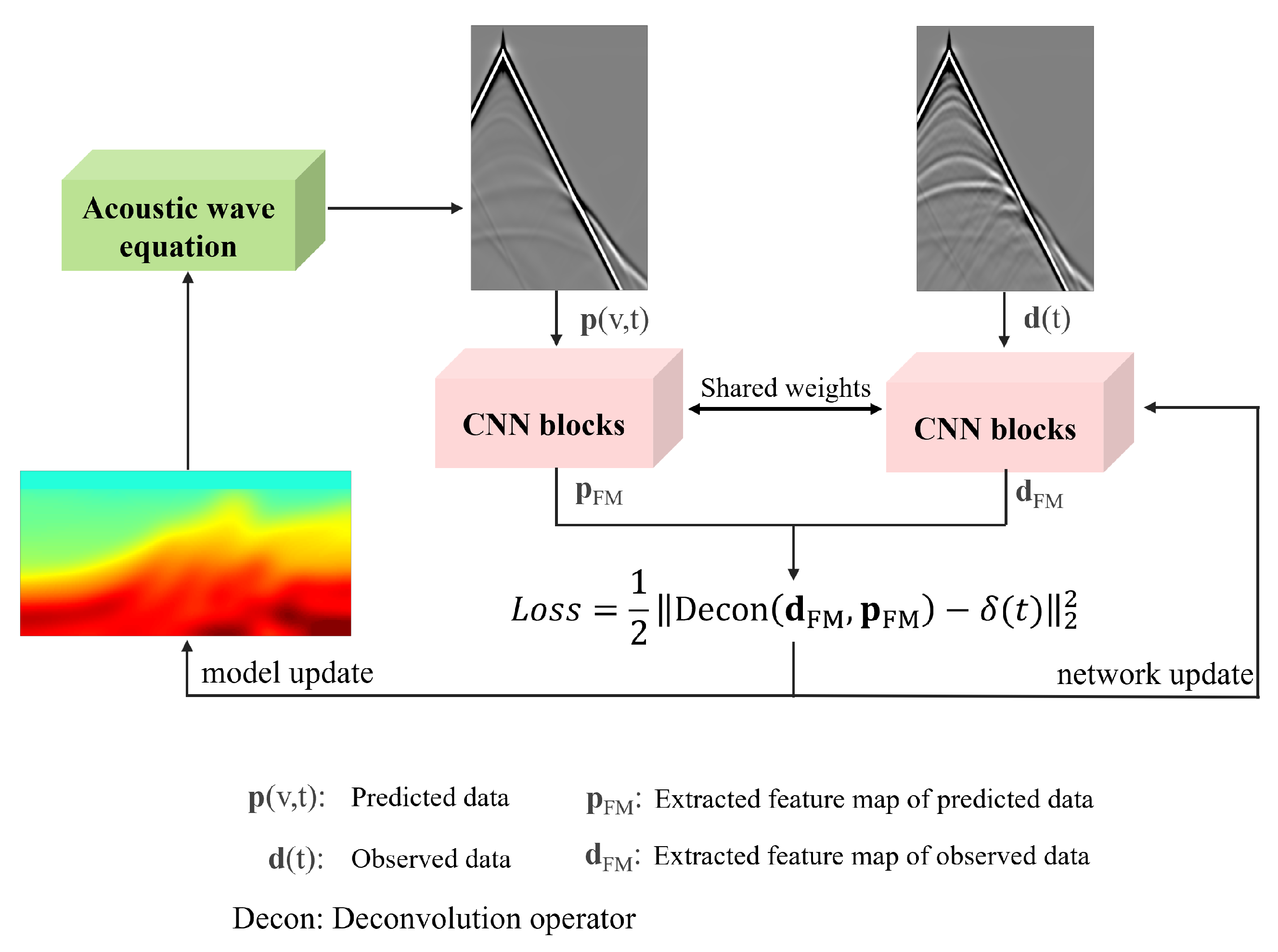
In detail, Figure 1 shows the workflow of the inversion process. First, the synthesized data p ( v curr , t ) and observed data d ( v real , t ) are input into the CNN blocks with shared weights to create feature maps p FM and d FM trace by trace in a latent space. Subsequently, a deconvolution-based loss function is used to update the velocity and network parameters simultaneously. Finally, using the updated velocity, we generate new predicted data and input the new predicted data and observed data into CNN blocks to obtain the refined feature maps. All steps are performed based on PyTorch 2.9.0 and the deepwave toolbox 0.0.20 [51].
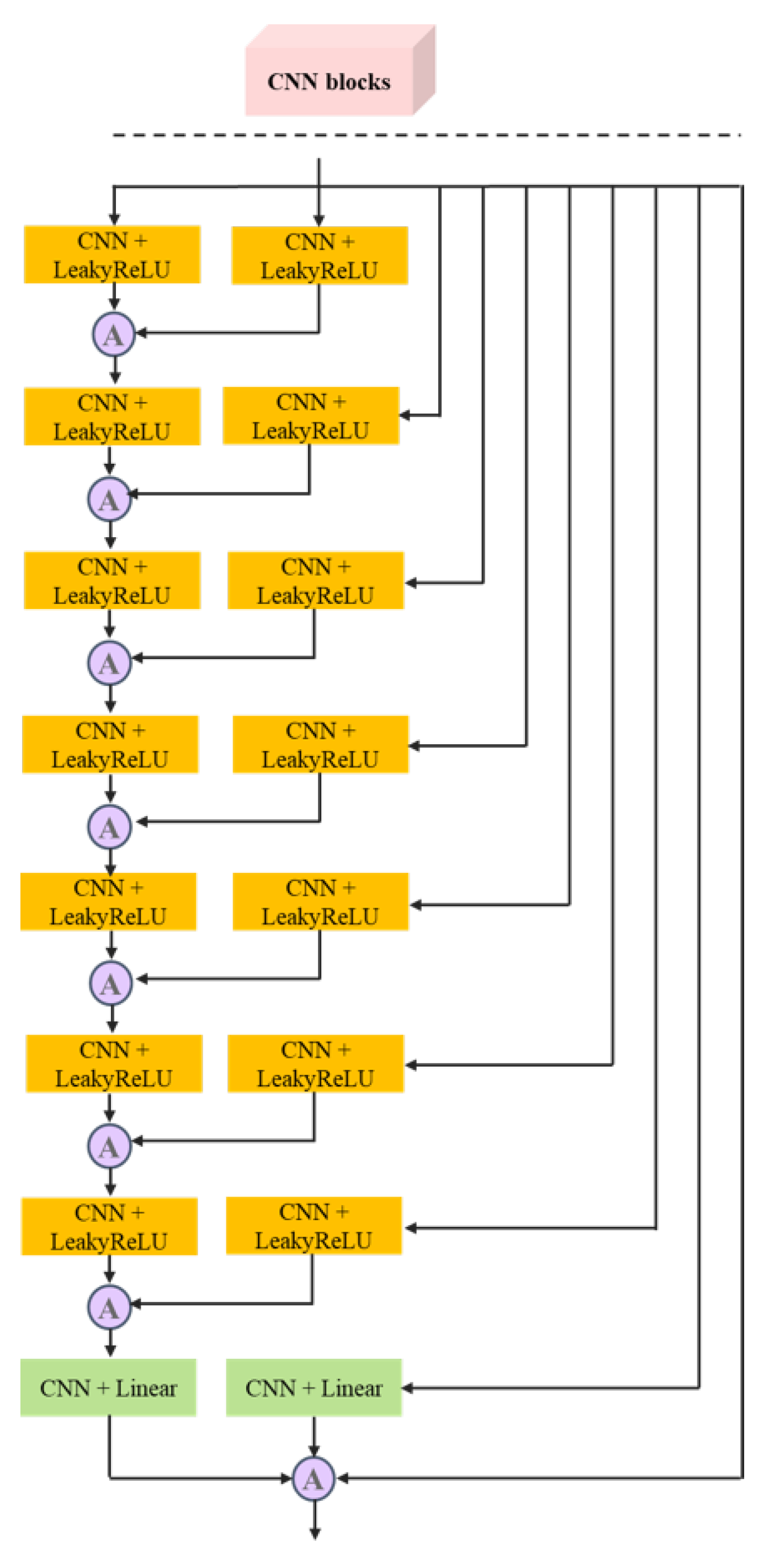
Figure 2 displays the detailed architecture of the CNN blocks. The architecture is relatively simple. We do not use any up- or down-sampling layers, so the extracted feature maps have the same size as the original input data. Reading from top to bottom, the number of extracted feature maps of each CNN layer is 1, 2, 2, 4, 4, 2, 1, and 1, respectively, and the convolution kernel size in each CNN layer is set to 3 × 3. Given an input vector s Ω N b × N t × N x , the input will first go through the main branch with eight consecutive CNN layers connected by addition operators, where N b , N t , and N x represent the batch size, the number of time samples, and the number of traces. Furthermore, eight additional CNN layers are connected to the output of each CNN layer in the main branch via skip connections. The summation of the output of each CNN layer in the main branch and the output of the corresponding skip connection will be fed into the next CNN layer. Mathematically, the output of the first seven CNN layers y i (e.g., i 1 7 ) can be expressed as
y i = σ W i m y i 1 + σ W i k s ,
where W i m and W i k are the weight matrix of the i-th CNN layers in the main branch and the corresponding skip connection. σ is the LeakyReLU activation function. Specifically, y 1 = σ W 1 m s + σ W 1 k s and the final output of the CNN block y 8 can be written as
y 8 = γ W 8 m y 7 + γ W 8 k s + s ,
where γ stands for the linear activation function. Equation (16) represents an improved data-fitting process, where the first two terms beginning with γ are the data-driven shaping constraints. Note that Equations (15) and (16) follow a ResNet-like residual learning paradigm and can mitigate the gradient vanishing problem. Meanwhile, the extra shaping constraints can counteract those components that are challenging to match after fine-tuning, leading to model updates and final inversion results.

3. Results

In this section, to demonstrate the superiority of the proposed DL-AWI, we will apply the proposed DL-AWI to two synthetic examples and a field example and compare it with the classic FWI method, classic AWI method [21], and the SiameseFWI [45], which are the state-of-the-art FWI algorithms. Specifically, SiameseFWI adopts Euclidean distance to build the misfit function. Classic AWI and DL-AWI use a deconvolution-based misfit function for inversion. All the experiments are conducted using an NVIDIA RTX 6000 GPU, and we use the Adam method to optimize the network and velocity model.

3.1. Marmousi Model

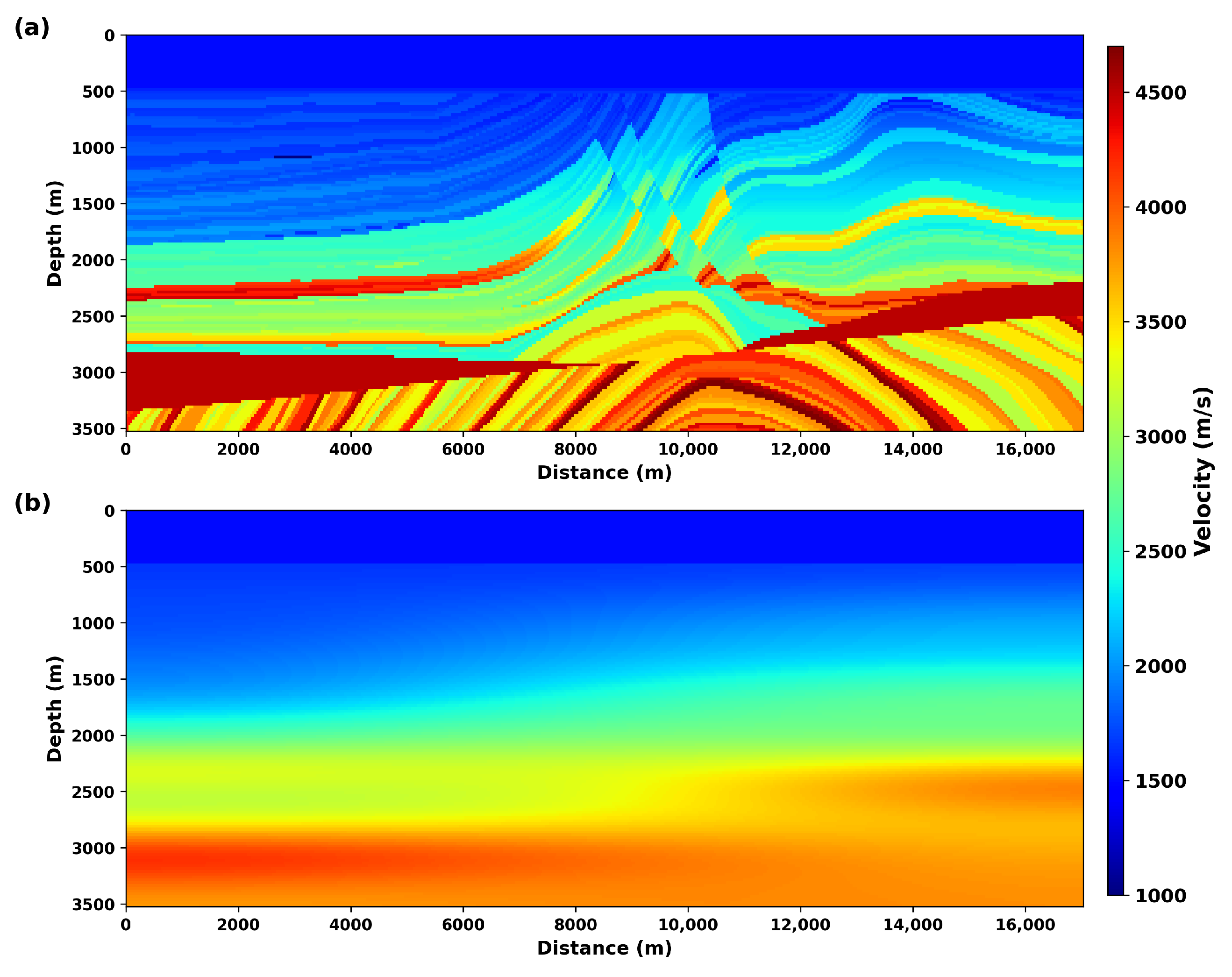
We first apply the proposed DL-AWI to the Marmousi model to evaluate the performance. The size of the velocity model is 141 × 681 with a sampling interval of 25 m, and we uniformly ignite 136 shots at the surface using a 5 Hz Ricker wavelet. The effective bandwidth range is approximately 2 to 8 Hz. Figure 3a,b show the real and initial models used for inversion, where we can see that the initial model is poor, which can result in cycle skipping if FWI is performed directly. During the inversion process, the number of iterations is set to 60, and the learning rates for the velocity update and network update are 5 and 0.0001, respectively.
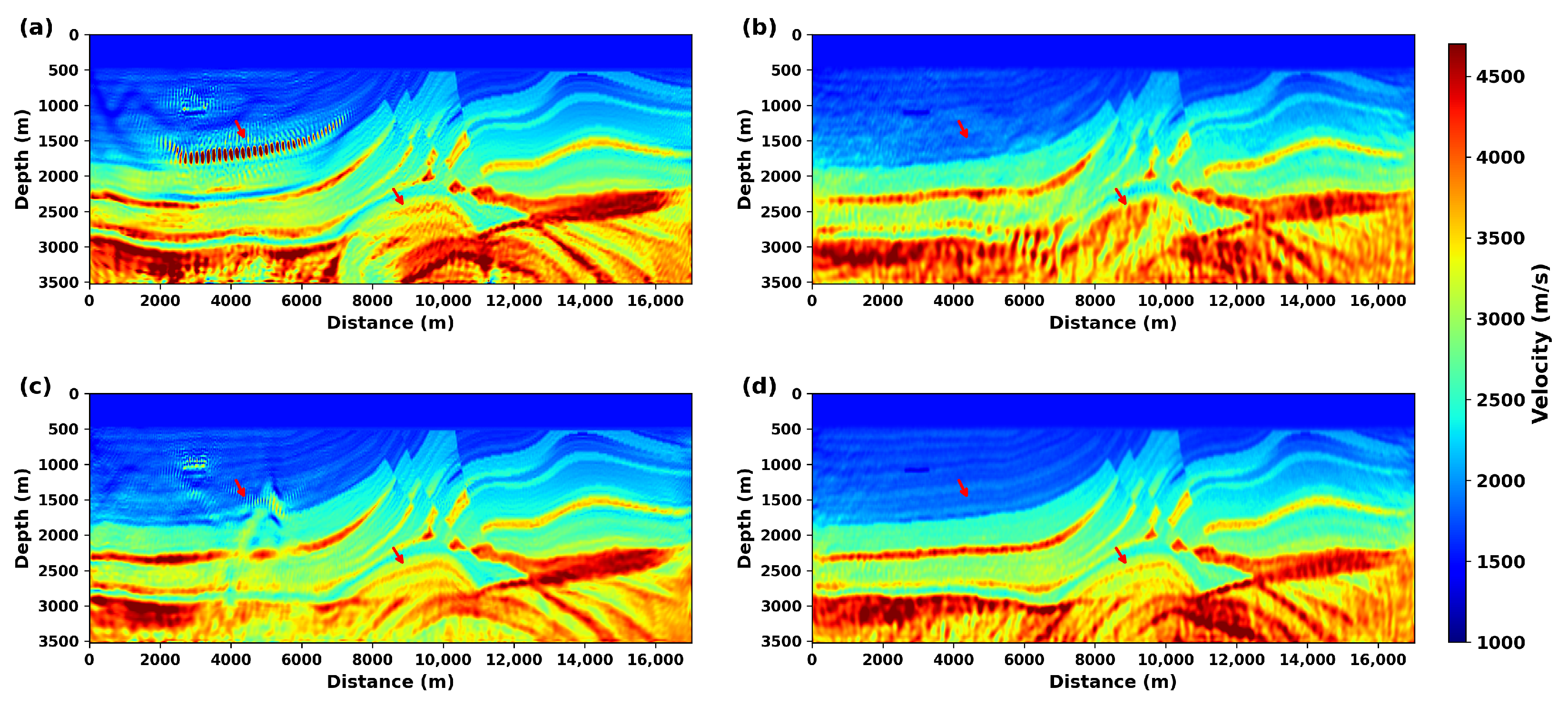
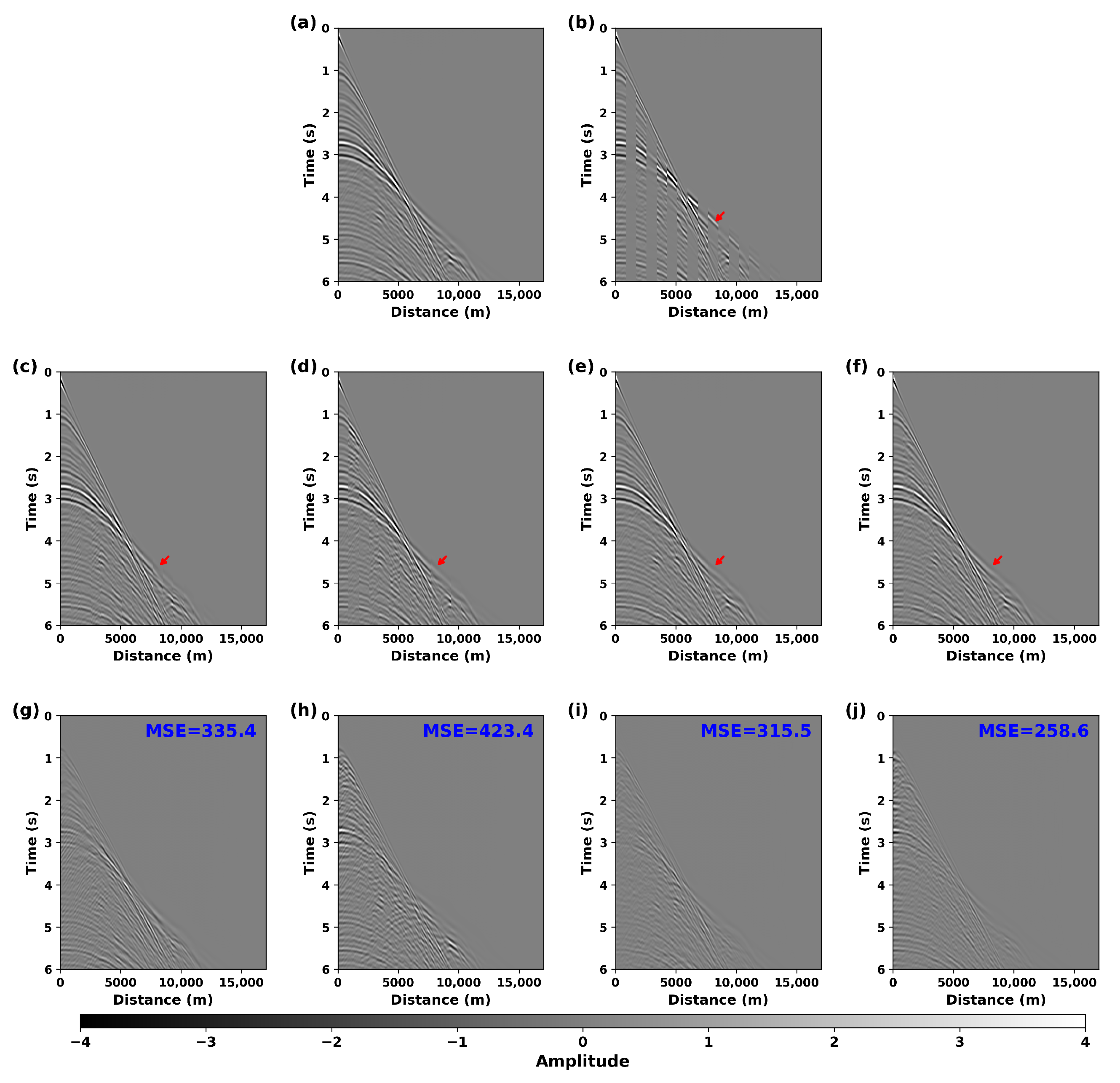
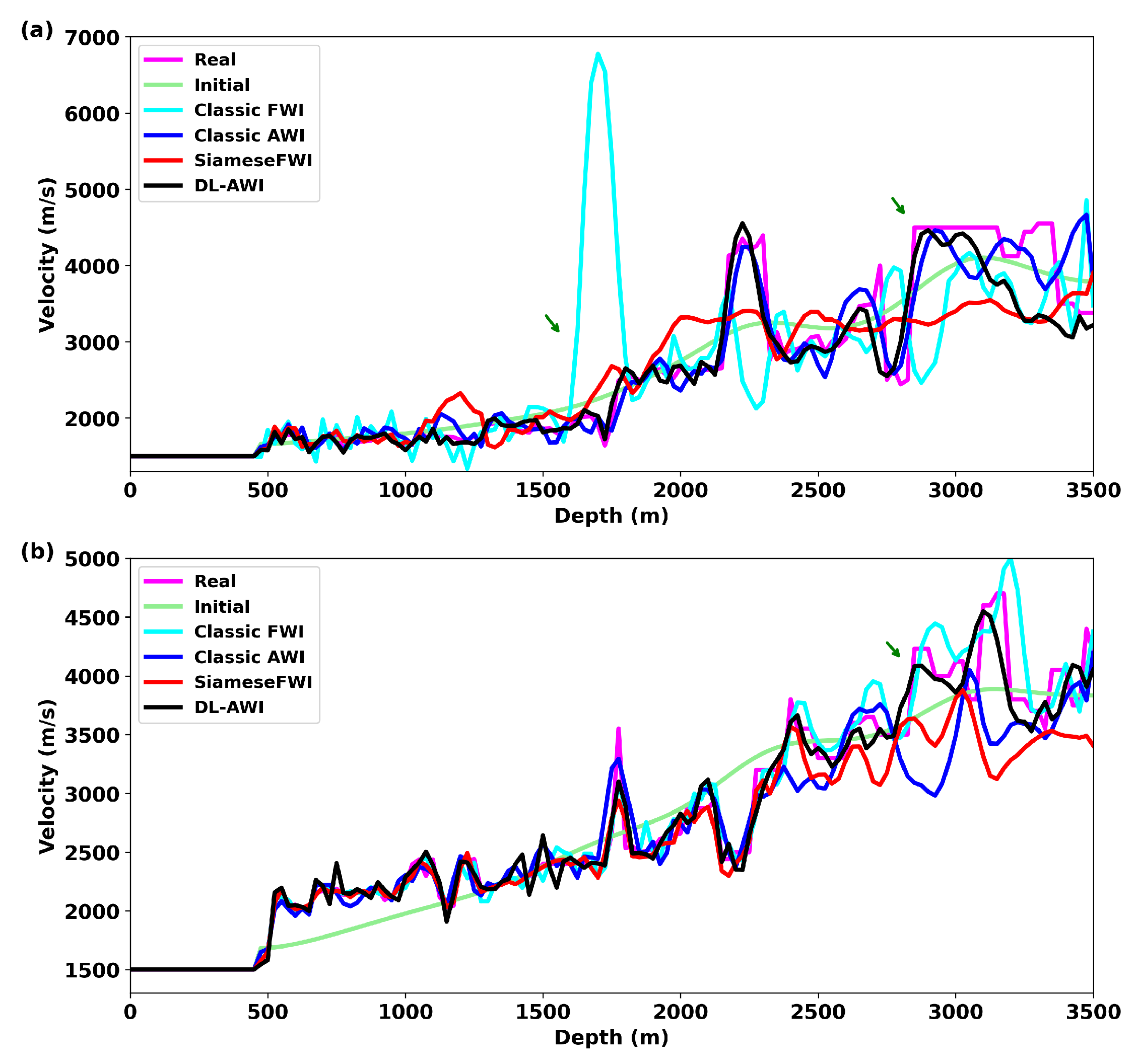
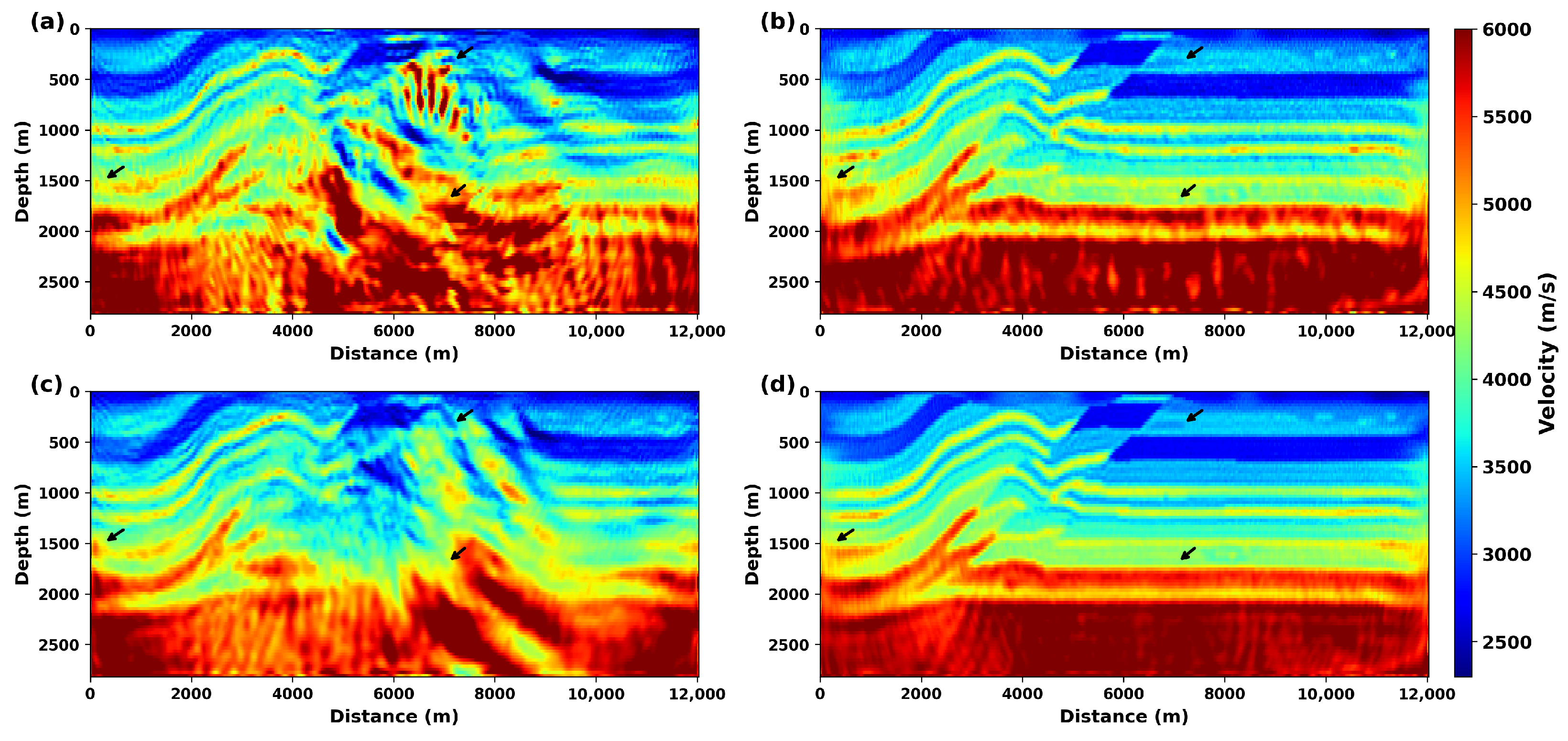
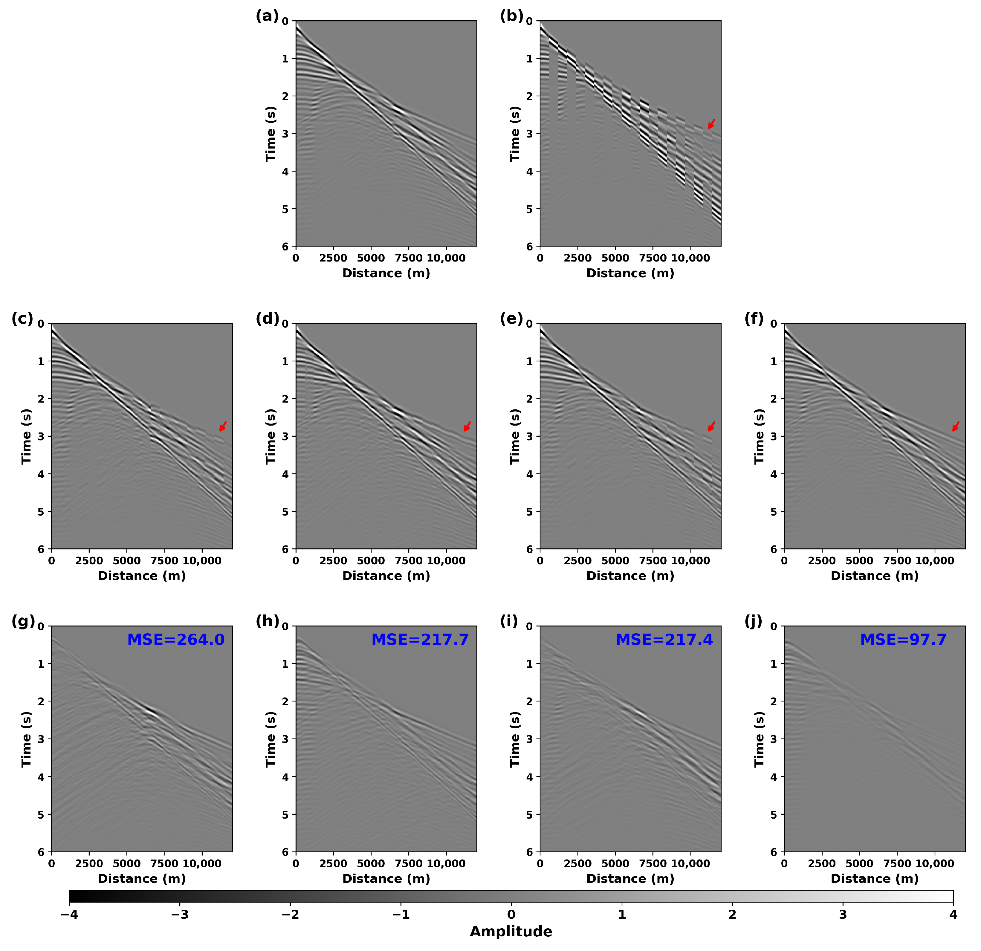
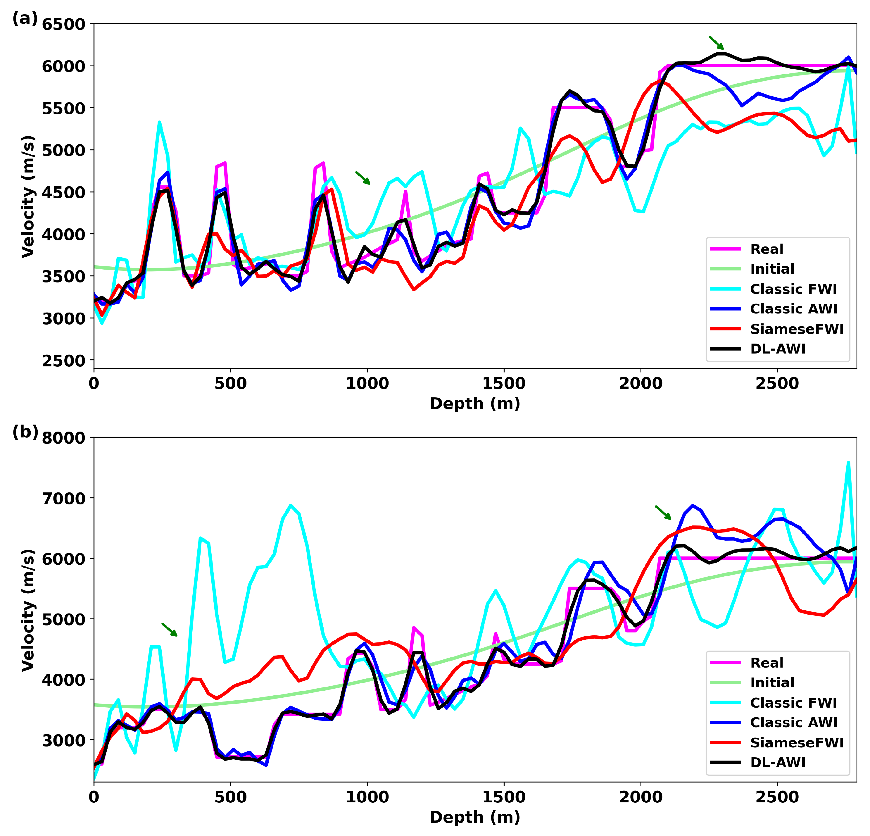
Figure 4 displays the inverted results using classic FWI, classic AWI, SiameseFWI, and DL-AWI. From a poor initial model, we find that the results in Figure 4a,c show more artifacts due to the effect of cycle skipping (e.g., highlighted by the red arrows), which demonstrates that classic FWI and SiameseFWI fail to provide reliable results. Figure 4b,d are the results of classic AWI and DL-AWI, where we can see that, compared with the real model, the inverted results are promising, indicating the robustness of classic AWI and DL-AWI. However, it is noticeable that the result of DL-AWI is cleaner than that of classic AWI. The result of DL-AWI displays more details (e.g., highlighted by the red arrows). Figure 5 compares the shot gathers generated using the real model, the initial model, and the inverted model. Note that from Figure 5b, we can see that the diving waves are mismatched at the far offset, indicating that the initial model is poor. Figure 5c–f show the interleaved shot generated by the real model and the inverted results using different methods. Obviously, at the far offset, we can see that the generated shot in Figure 5f shows an improved continuity and similarity (e.g., marked by red arrow), demonstrating that the inverted result of DL-AWI is more reliable. Figure 5g–j show the final data residual corresponding to different benchmarks, where we can see that DL-AWI can lead to a lower mean squared error (MSE), which means that DL-AWI can converge faster under the same conditions. To provide an intuitive comparison, we extract two vertical profiles from Figure 4 at distances of 4000 m and 10,000 m, and the results are displayed in Figure 6. It is apparent that although the accuracy of DL-AWI decreases at greater depths compared with the ground truth (magenta line), its performance (black line) remains visually superior to that of the other benchmark methods. We use the green arrows to highlight the obvious improvements, demonstrating the superiority of the proposed DL-AWI.
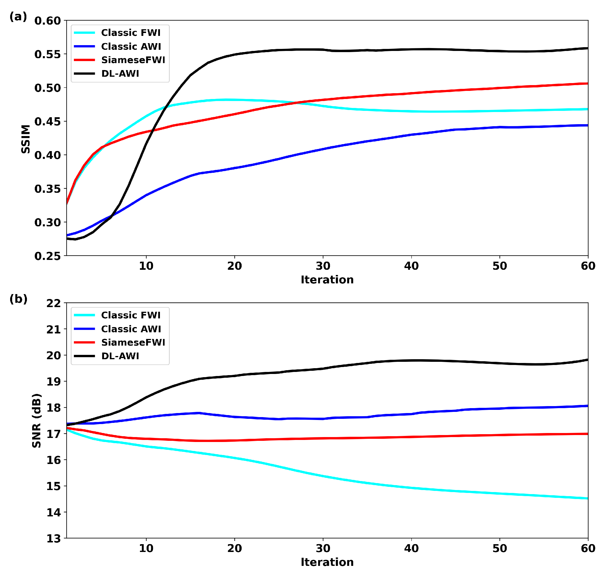
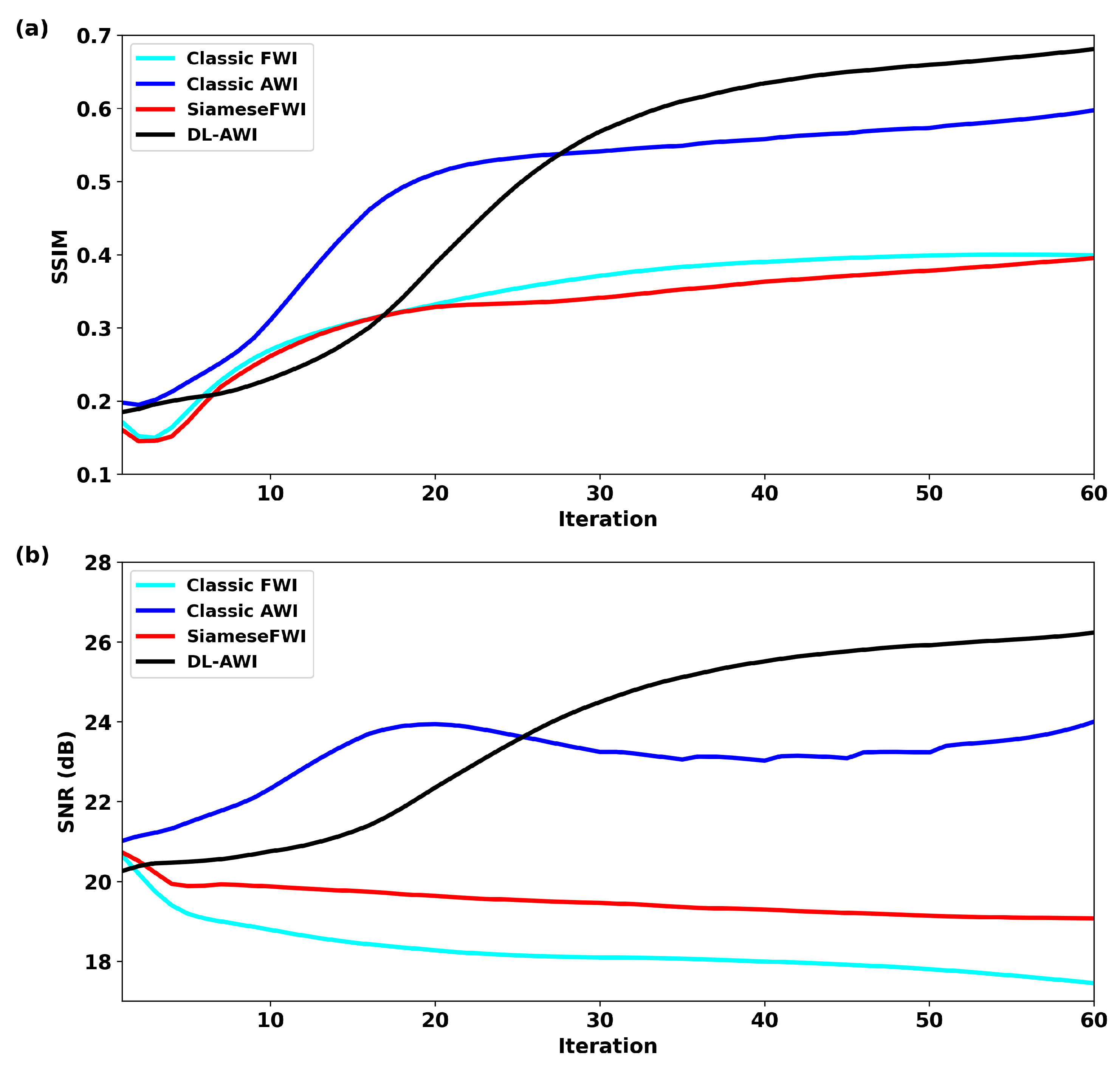
Moreover, we also use the signal-to-noise ratio (SNR) and structure similarity index measure (SSIM) to quantify the inverted results. Figure 7 depicts the SNR and SSIM variation curves of the Marmousi model with an increasing number of iterations. In detail, from Figure 7a, we can find that the increasing rate of SSIM curves of classic FWI and SiameseFWI will decrease gradually, which means that it is challenging for classic FWI and SiameseFWI to update the current model toward the real model. As for the SSIM curves of classic AWI and DL-AWI, we observe that they increase as expected, and DL-AWI accelerates model updates for the same number of iterations, validating its improved efficiency. Figure 7b is the SNR variation curve. We find that the SNR variations corresponding to classic FWI and SiameseFWI are small because, when trapped in local minima, they cannot progressively correct the gradient error. Furthermore, we observe that the curves for classic AWI and DL-AWI increase. However, with the help of the deep twin network, DL-AWI can benefit from data fitting during data matching after fine-tuning, providing improved results.

3.2. Overthrust Model

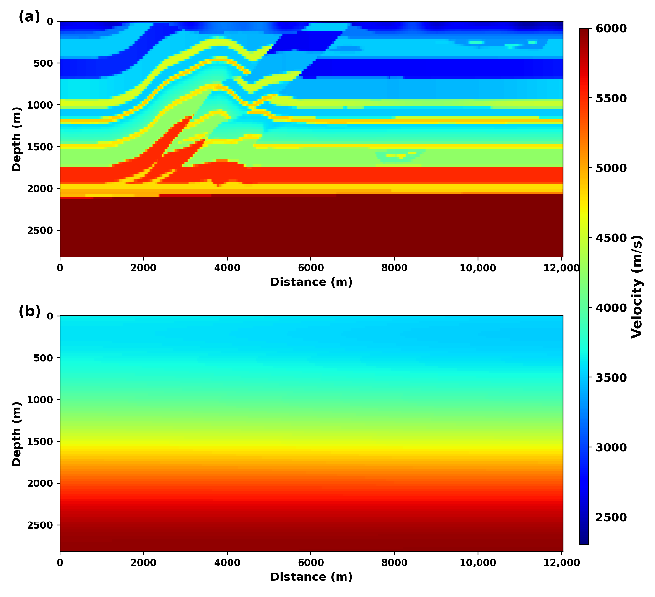
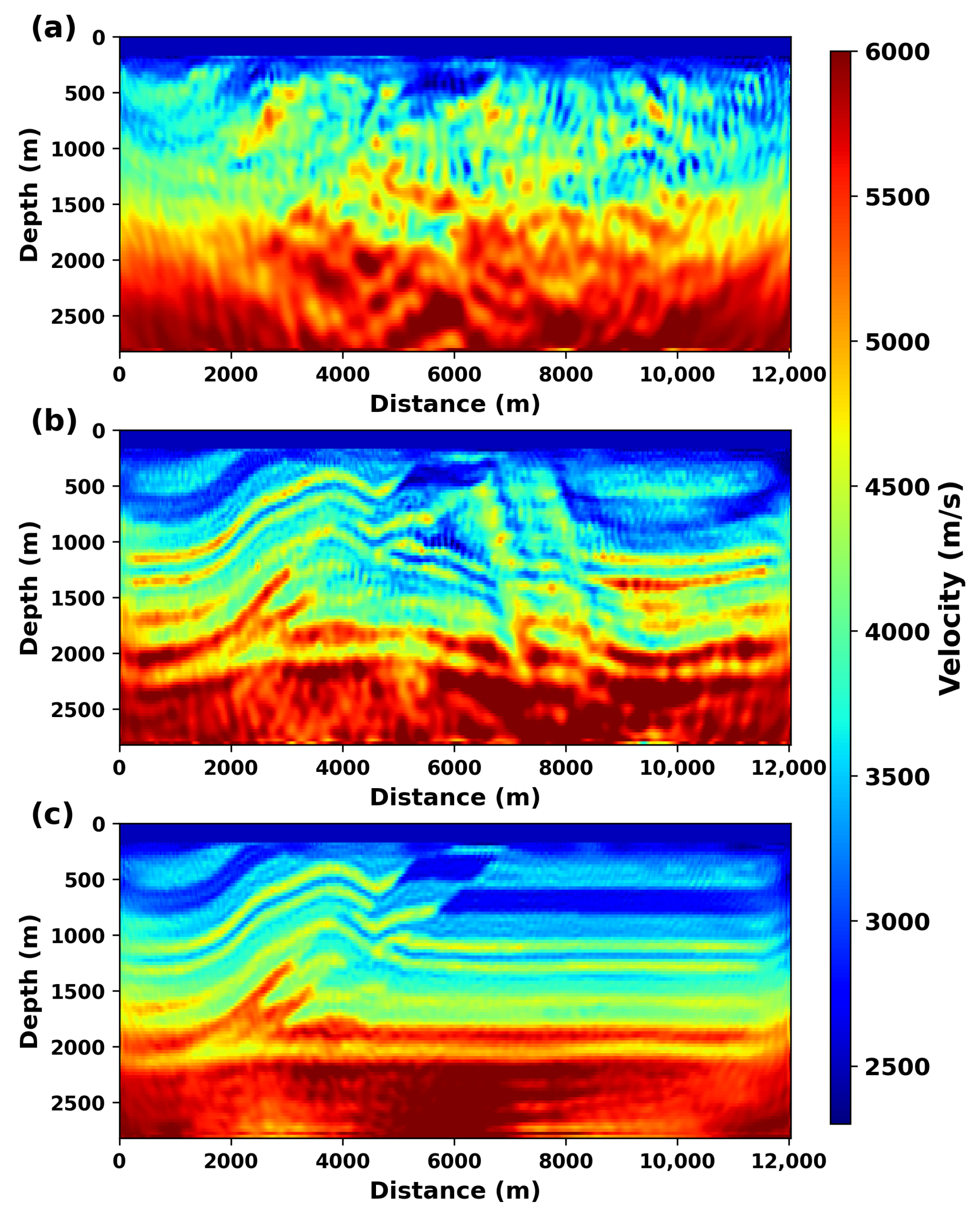
We then use the SEG/EAGE overthrust model to compare the efficacy of the proposed DL-AWI with benchmarks. We uniformly generate 80 shots at the surface with a 5 Hz Ricker wavelet because a 5 Hz wavelet contributes to the robustness of the inversion process, and we will discuss the choice of wavelet in the discussion section. The model size is 94 × 401 with an interval of 30 m, and the other parameters are unchanged. Figure 8a shows the real model, and Figure 8b is the initial model used in the experiment. The poor initial model will cause cycle skipping. Figure 9 shows the inverted results using different methods. Comparing classic FWI, classic AWI, and SiameseFWI with DL-AWI, it is obvious that the result of DL-AWI shows improved accuracy and resolution. Due to the poor initial model, although classic FWI and SiameseFWI cannot recover the real model, we find that SiameseFWI can suppress some artifacts during the inversion process to some extent with the help of the deep neural network. Figure 9b,d show the inverted results of classic AWI and DL-AWI, respectively. It is apparent that the result shown in Figure 9d is more accurate, especially at the edge and deep positions (e.g., highlighted by the black arrows). The result of AWI shows obviously abnormal lower values at the bottom left corner, and such a phenomenon may be caused by the complexity of globally matching using AWI. As for DL-AWI, it will match the mapped predictions and the observations in an extended latent space, where more attention will be paid to local signal features. Figure 10 displays the generated shots using the real model, the initial model, and the inverted model corresponding to different benchmarks. From Figure 10b, we can see that the shot waveform at the far offset is mismatched, indicating that the initial model is poor. Figure 10c–f compare the real shot with the predicted shot created using the inversion results of different methods. In particular, we can find that the shot in Figure 10f shows improved similarity. Figure 10g,j depict the final data residual corresponding to classic FWI, classic AWI, SiameseFWI, and DL-AWI, respectively. It is obvious that the data residual shown in Figure 10j is the lowest, indicating that DL-AWI provides a more accurate inversion result.
Figure 11 shows the extracted vertical profiles at different positions from Figure 9 for further comparison. Compared with the real model, we can easily find that the result of DL-AWI is superior in terms of accuracy in both Figure 11a,b. Classic FWI and SiameseFWI are trapped in the local minima, and we can see that the inverted velocity models (cyan and red lines) are far away from the real model (magenta line). Additionally, although classic AWI performs better than classic FWI and SiameseFWI, it results in more errors at a depth of 2200 m than DL-AWI as shown in Figure 11b, which demonstrates that DL-AWI is more effective and robust under the same circumstances. Figure 12 shows the SSIM and SNR curves corresponding to the second synthetic example. SSIM considers changes in local structure information, and SNR mainly focuses on the amplitude fidelity. Both of them can evaluate the accuracy of the inverted results from different perspectives. Obviously, although the SSIMs corresponding to classic FWI and SiameseFWI increase, the final results are not accurate due to the cycle skipping problem. In contrast, classic AWI and DL-AWI are both effective for recovering the velocity model and, notably, DL-AWI exhibits a higher convergence rate than classic AWI. As for the SNR curves shown in Figure 12b, we can see that classic FWI and SiameseFWI lead to inferior results with lower SNRs. Compared to classic AWI, DL-AWI offers a better velocity model, and more iterations are required for classic AWI to achieve the same performance. Both the SNR and SSIM validate the great efficiency and robustness of DL-AWI.

3.3. Field Data

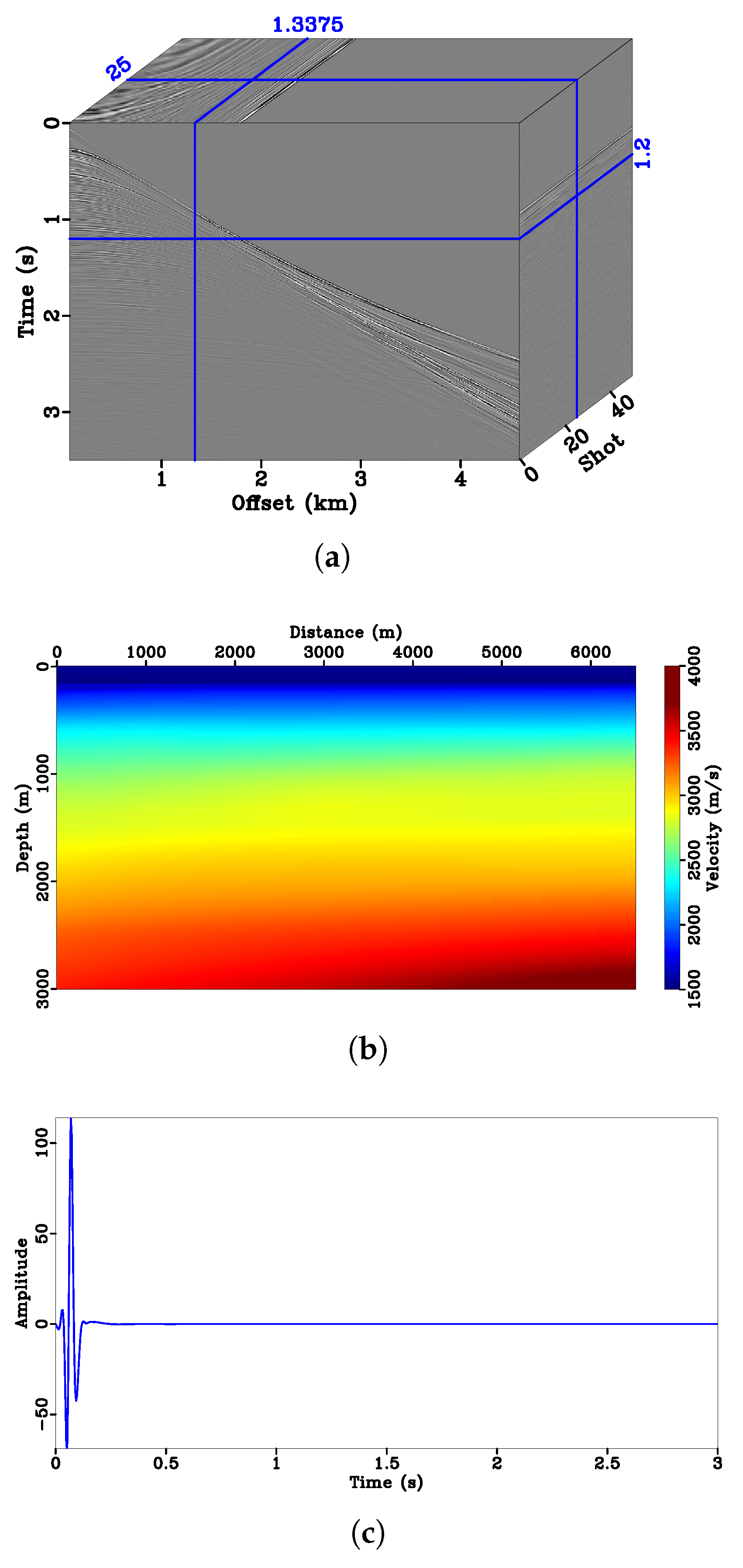
In this section, we use a field example from the South China Sea to evaluate the effectiveness of DL-AWI. The field data comprises 50 shots with an interval of approximately 100 m. Each shot gather contains 360 traces, and the offset ranges from 0.0875 km to 4.5875 km. Figure 13 shows the original shot gathers, the initial velocity model, and the corresponding source wavelet. Then, we apply a bandpass filter to the original dataset to extract the signals ranging from 5 to 10 Hz for inversion. During the experiment, we also keep the learning rates for velocity update and network update unchanged and perform inversion for 15 iterations.
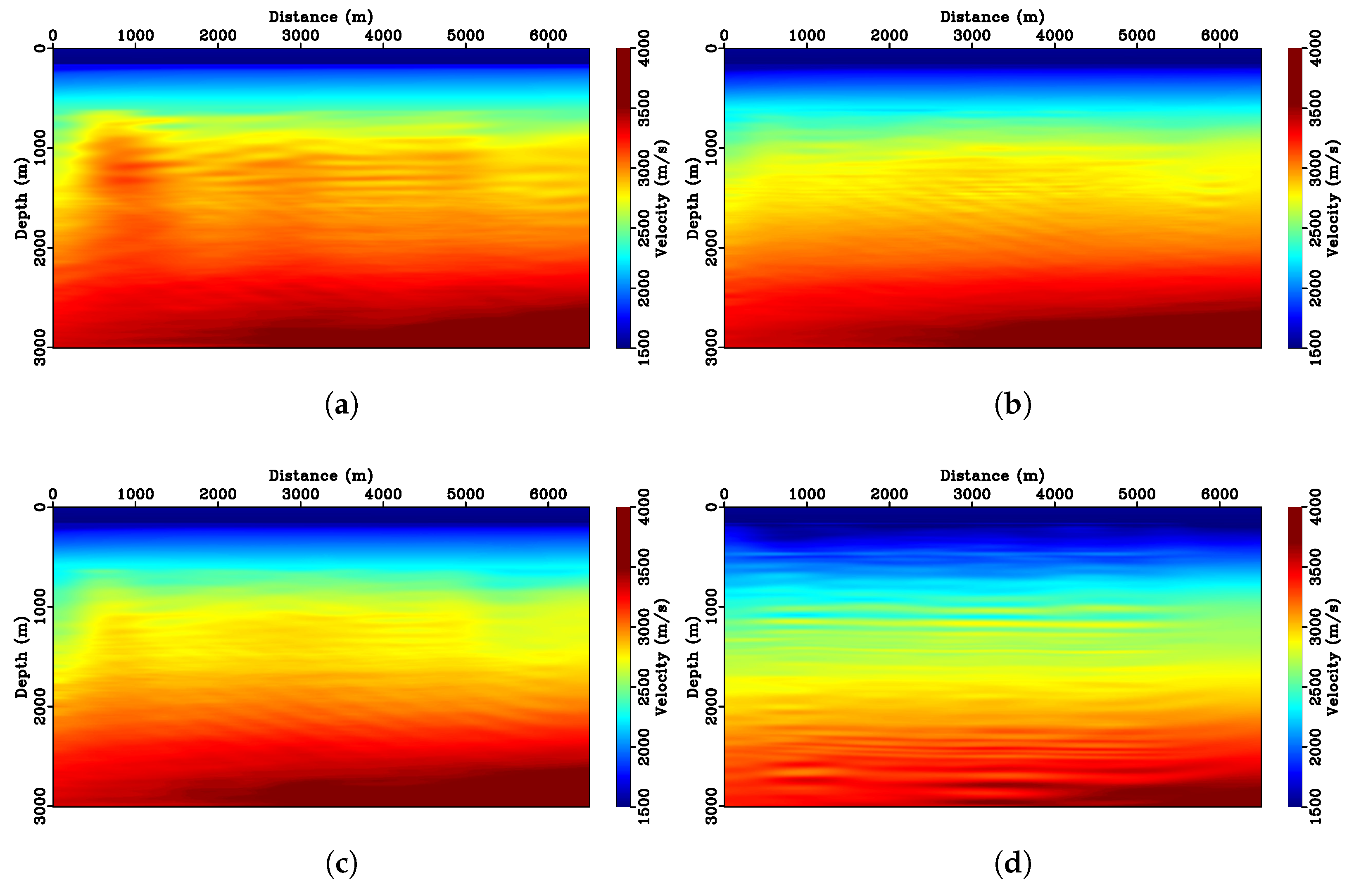
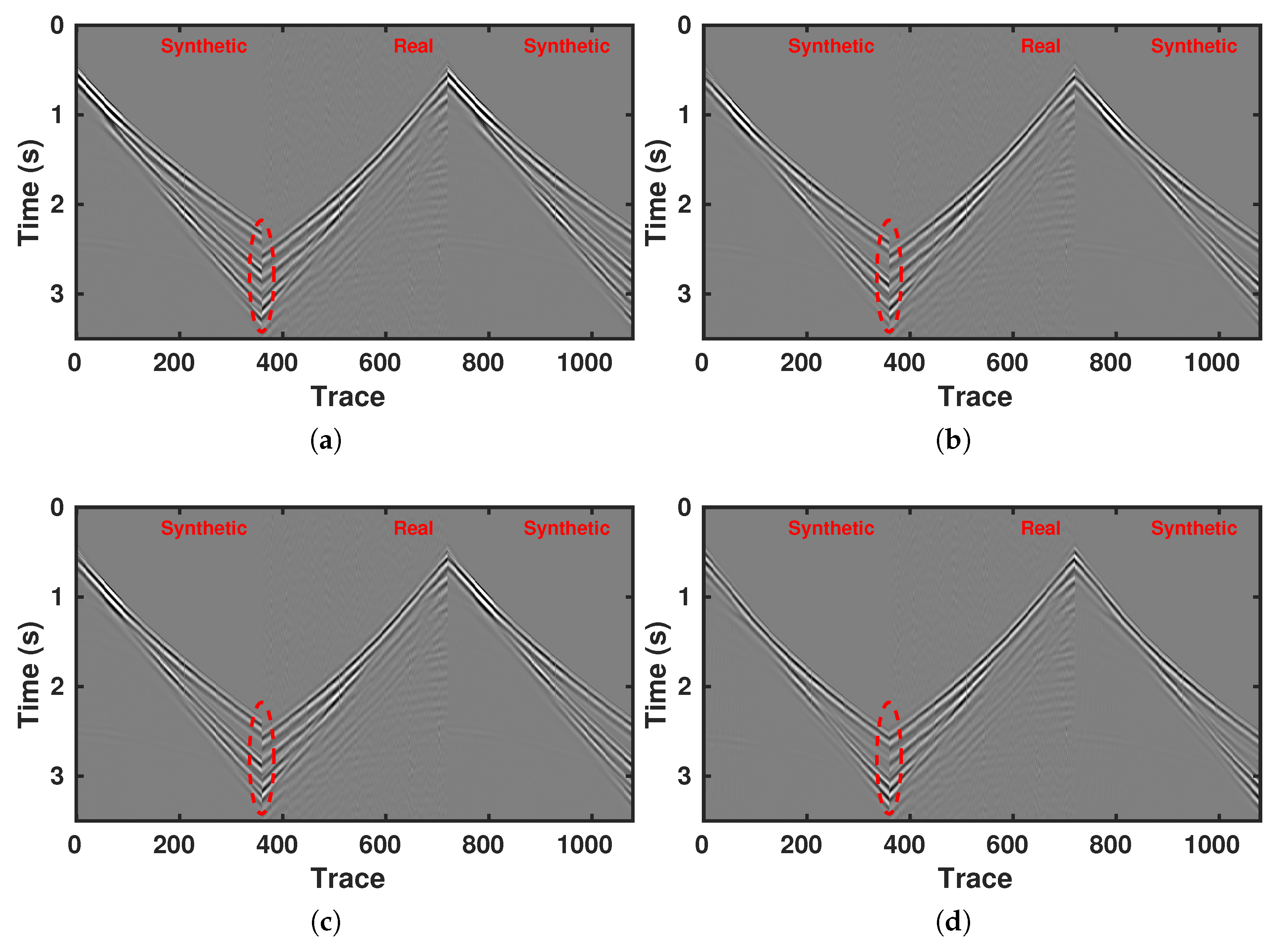
Figure 14 shows the inverted velocity model using classic FWI, classic AWI, SiameseFWI, and DL-AWI, respectively. Compared with the initial model, the background velocity values shown in Figure 14b,d decrease. The velocity values in Figure 14a,c increase slightly. To evaluate the accuracy of the inverted velocity models in Figure 14, we generate synthetic diving waves using the inverted models and compare them with the real diving waves. Figure 15 shows the results of the diving wave comparison. Figure 15a compares the real and synthetic diving wave after classic FWI, where we can see an obvious mismatch at the far offset (e.g., highlighted by the red ellipse). Due to the effect of cycle skipping, classic FWI cannot provide an accurate result. Figure 15b–d display the real and synthetic diving waves after classic AWI, SiameseFWI, and DL-AWI. By careful observation, we can see that the time difference between real and synthetic diving waves is completely corrected by DL-AWI, demonstrating its efficacy and robustness. Although classic AWI and DL-AWI can mitigate the mismatch, DL-AWI is more efficient with the same number of iterations, thereby reducing the computational cost of the inversion process.
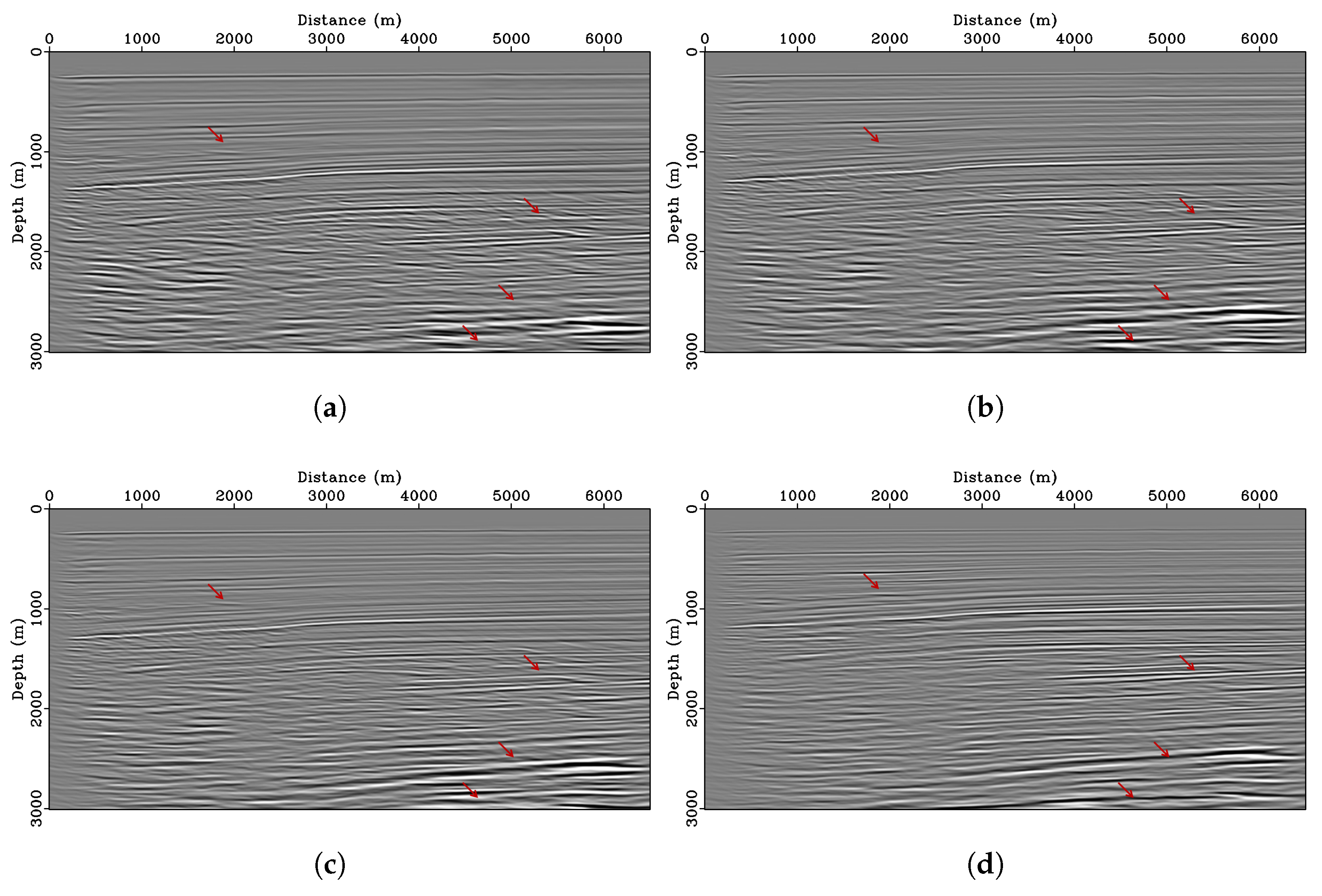
Next, we conduct Kirchhoff prestack depth migration (PSDM) using the inverted velocity models to evaluate the contribution of the velocity model to the image. Figure 16 displays the migration profiles corresponding to velocity models obtained by different methods. Comparing Figure 16d with Figure 16a–c, it is obvious that the velocity obtained by DL-AWI can lead to a better visual quality with improved resolution (e.g., highlighted by the red arrows). Notably, compared with Figure 16a, although we can see that the image quality improves in Figure 16b,c at the right corner, the ability of classic AWI and SiameseFWI to alleviate cycle skipping is inferior and less efficient than that of DL-AWI. Figure 17 shows the extracted offset domain common image gather (ODCIG) at different locations. It is intuitive that the events in Figure 17d are almost flattened, validating the reliability of the inverted velocity using DL-AWI. Compared with Figure 17a, we find that the events in Figure 17b,c are still curving, which demonstrates the suboptimal efficacies of classic AWI and SiameseFWI when dealing with cycle skipping.

4. Discussion

In this section, we discuss the robustness of the proposed DL-AWI and provide some caveats for its practical applications. All the experiments are based on the Overthrust model shown in Figure 8.

4.1. Dependence on Initial Models

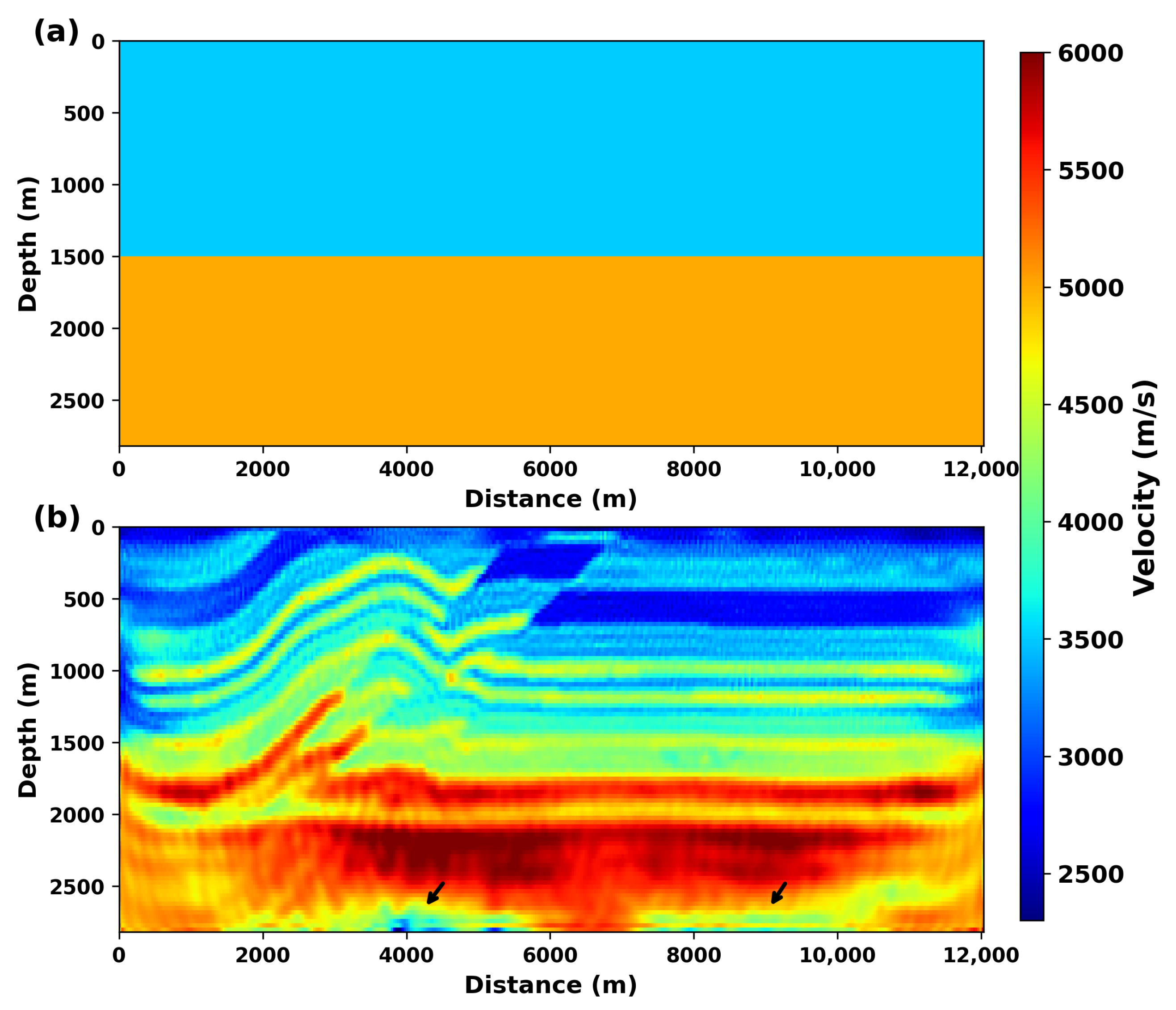
First of all, we analyze the sensitivity of DL-AWI to initial models. We create a fairly poor initial model for inversion, as shown in Figure 18a, which is a simple layered constant-velocity model with velocities of 3500 m/s and 5000 m/s. We conduct DL-AWI for 60 iterations and keep the other parameters unchanged. Figure 18b shows the final inversion result based on Figure 18a. Surprisingly, the inversion result is satisfactory. To quantify the inverted result, the SNR and SSIM corresponding to Figure 18b are 19.33 dB and 0.66, respectively. Note that although the accuracy is relatively low at some bottom positions, the inversion validates that DL-AWI can significantly mitigate the strong dependence of FWI on a good initial model and demonstrates the potential to obtain reliable results under extreme conditions.

4.2. The Influence of Low-Frequency Components and Bandwidth

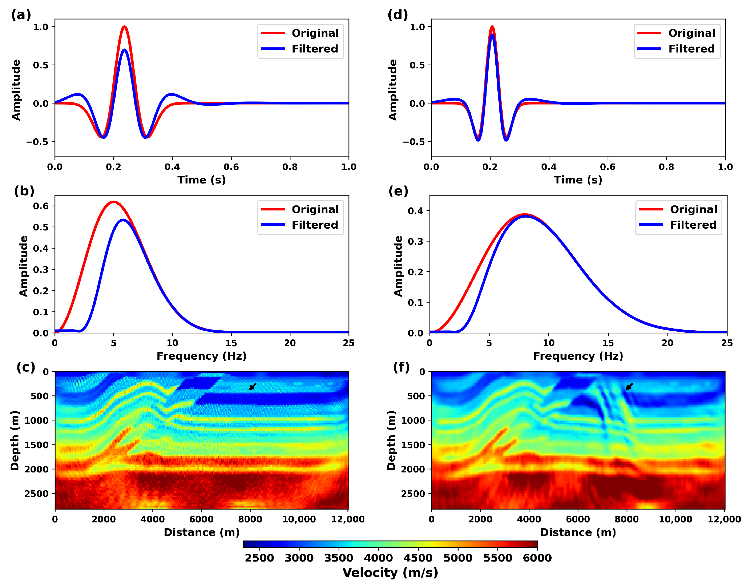
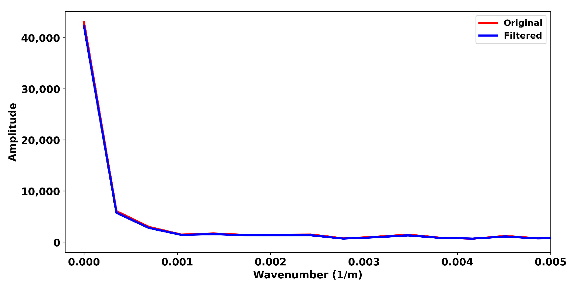
Moreover, we will analyze the influences of low-frequency components and frequency bandwidth on the proposed DL-AWI because they are important factors. To evaluate the influence of low-frequency components, we first filtered the components below 3 Hz in the wavelet, and the corresponding waveform and spectrum are displayed in Figure 19a,b. Based on the initial model shown in Figure 8b, Figure 19c shows the final inversion result inverted using a filtered 5 Hz Ricker wavelet, where we can see that DL-AWI is robust and can also provide reliable results when the low-frequency components are missing. Then we use an 8 Hz wavelet and filter those components below 3 Hz. The corresponding wavelet and spectrum are shown in Figure 19d,e. Figure 19f displays the final inversion result using the filtered 8 Hz wavelet, where we can see some obvious artifacts (e.g., marked by the black arrow) due to the poor initial model. In reality, we suggest using a multiscale scheme to conduct inversion. We can begin with low frequencies (e.g., 3 Hz) and gradually add higher-frequency components to improve accuracy and resolution. At the early inversion stage, incorporating more high-frequency components may yield inferior results. Moreover, Figure 20 shows the spectrum of the inverted velocity shown in Figure 9c,d. The inversion results are obtained using a 5 Hz wavelet with and without low-frequency components. It is clear that the spectrum matches with each other, indicating that the proposed DL-AWI can recover low-wavenumber components for the velocity model and is less dependent on the low-frequency components in the raw seismic data.

4.3. Noise Level Influence

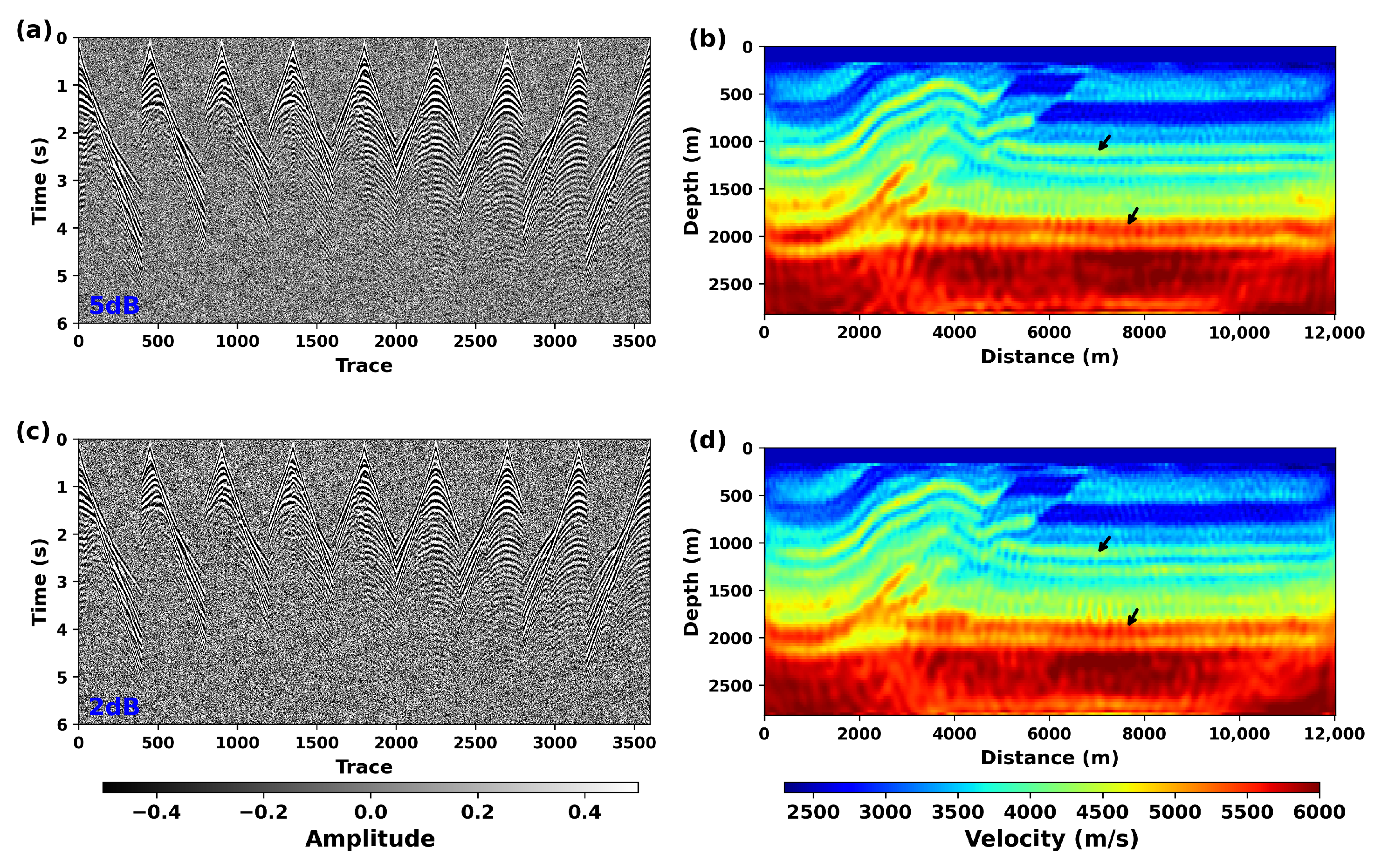
Additionally, the noise level can also influence the final performance of DL-AWI. Based on the Overthrust model, we generate noisy data with different noise levels (e.g., 5 dB and 2 dB) and conduct inversion to assess the effects of noise based on Figure 8b. Figure 21 shows the noisy data and the corresponding inversion results, where the final model SNR and SSIM of the inverted results are 24.01 dB, 23.32 dB, 0.55, and 0.52, respectively. Intuitively, compared to the reference model shown in Figure 9d, we can recognize that although the accuracy and resolution of the final inversion result will degrade with increasing noise level (for example, marked by black arrows), the proposed DL-AWI is also able to suppress artifacts related to the poor initial model.

4.4. Computational Cost Analysis

In addition, we compare the computational costs of classic FWI, classic AWI, SiameseFWI, and DL-AWI. Based on the inversion results shown in Figure 9, the corresponding computational times are 321 s, 377 s, 319 s, and 324 s, respectively. Notably, compared with classic FWI and AWI, the proposed DL-AWI incurs only a small additional computational burden. Currently, all the experiments in the manuscript are based on 2D data. Regarding 3D FWI, we expect the computational cost to increase, and we will make addressing this issue a major focus of our future research.

4.5. Ablation Tests and Architecture Analysis

Next, we will perform ablation experiments to evaluate the architecture of the deep neural network. In our first ablation experiment, we remove all the skip connections in the CNN blocks and conduct the inversion process with the other parameters unchanged. Figure 22a shows the final inverted result, where we can see that the inverted result is less accurate and contains more artifacts. The final SNR and SSIM of Figure 22a are 18.3 dB and 0.21, respectively. We believe that skip connections are helpful and necessary for DL-AWI because the network weights are randomly initialized, which cannot guarantee that the network will build a wide latent space that includes the global convergence region. The additional skip connections can provide sufficient original information to mitigate instability in the early stages of the inversion process [32]. Furthermore, we also assess the influence of the number of CNN layers used for inversion. Based on Figure 2, we change the number of CNN layers to 5 and 10 and reconduct the inversion. Figure 22b,c are the inverted results, and the corresponding SNR and SSIM are 19.2 dB and 0.32 and 24.6 dB and 0.64, respectively. Obviously, fewer CNN layers may prevent the network from extracting the most relevant signals for data matching, leading to suboptimal results. Moreover, compared with the result shown in Figure 9d, increasing the number of CNN layers does not yield visible improvements. In most cases, eight CNN layers are suitable in terms of accuracy and computational cost. Regarding the architectural design, more complex models (e.g., Transformer-based architectures) could potentially achieve better global data fitting. However, in practice, it is not necessary to completely eliminate the mismatch between the predicted and observed data. Instead, it suffices to construct a simple, compact filter to correct phase differences exceeding half a cycle, which is sufficient to ensure the stability of the inversion. Although a Transformer-based model may achieve comparable performance, FWI is already computationally expensive, and adopting such architectures would further increase the computational burden.

4.6. Interpretation of the Inversion Mechanism

The principle of the deep twin network in the DL-AWI algorithm is to extract the most distinct components in the synthetic and observed data for misfit calculation so that the iterative inversion process will only focus on the most dominant wave components (e.g., direct and refracted waves) in early iterations. Later on, as the gradient-based inversion process (left part in Figure 1) recovers more velocity details, the synthetic data will contain more complicated wave components (e.g., diving and reflected waves). The deep twin network will further extract the more complicated wave components for misfit calculation [45]. This strategy is analogous to the multi-scale inversion scheme, which has been demonstrated to overcome cycle-skipping issues, albeit to a limited extent, in a completely data-driven, neural-network-guided manner. This approach can also be understood as a concatenated traveltime tomography and full waveform inversion framework, all through the inclusion of convolutional neural networks. By including more complex wave components across epochs, the proposed DL-AWI gradually recovers the lowest-wavenumber velocity model and then the higher-wavenumber velocity model components. Similar ideas have also been explored in the global seismology community by designing the time windows to extract the most distinct components over the iterations [52]. However, here, we leverage CNNs for adaptively choosing these “time windows” as well as correcting their time shifts and amplitude errors.
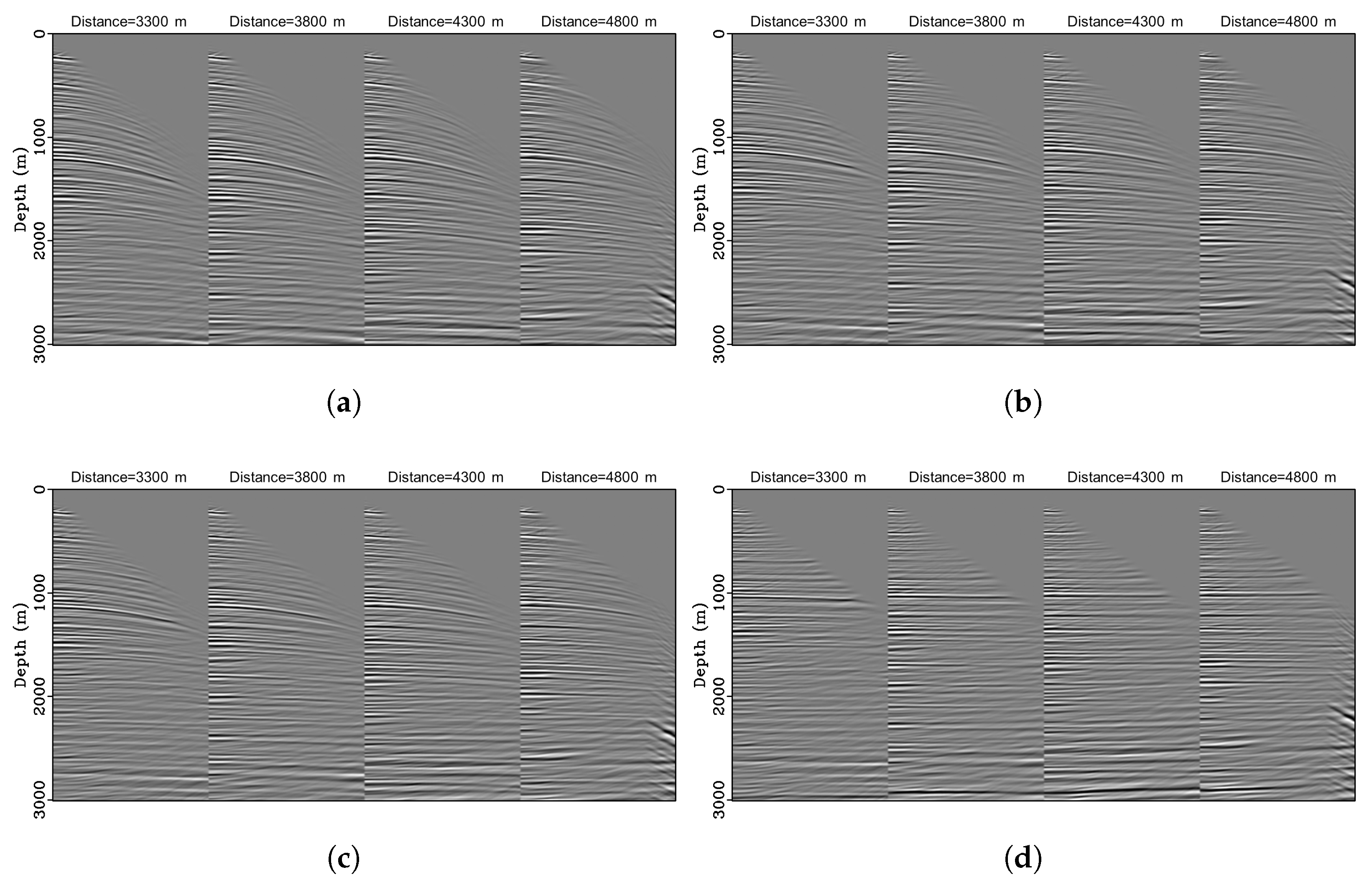
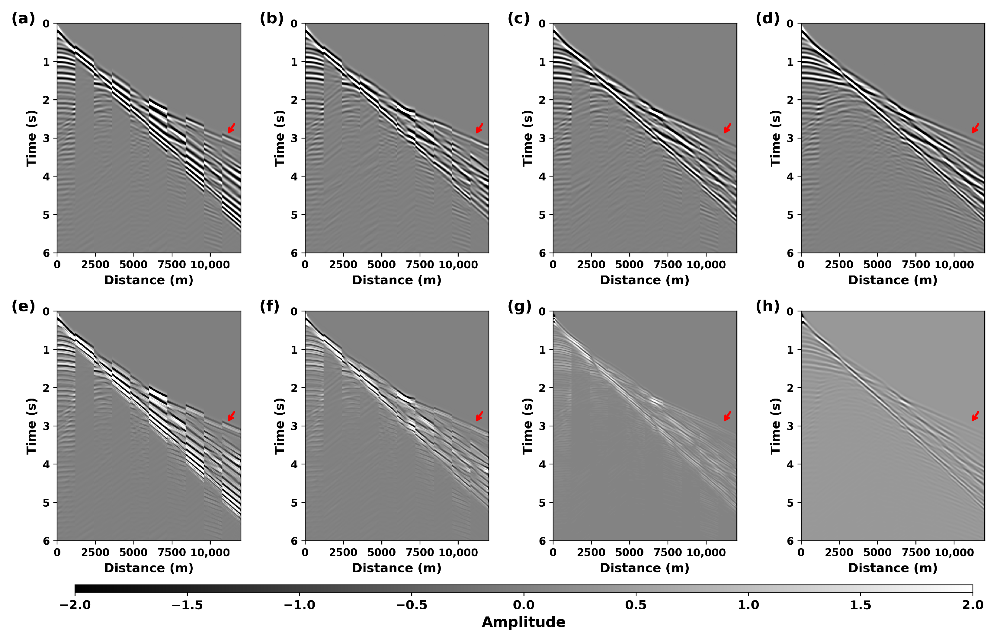
In detail, Figure 23 shows the original predicted and observed data and their extended version in an interleaved manner. Figure 23a–d show the original observed and predicted data with an increasing number of iterations, where we can see obvious waveform differences in terms of energy and phase. Specifically, Figure 23e–g show the extended observed and predicted data in the latent domain with the increasing number of iterations. Unlike the original data, we can see that the amplitude discrepancy decreases after network mapping. The network provides a robust environment for data matching by balancing the amplitude difference between the predicted and the observed data, facilitating the process of data matching. More importantly, the balanced data can effectively contribute to the accelerated convergence rate of the deconvolution-based objective function. During the whole inversion process, we can see that DL-AWI can deal with amplitude and phase mismatches simultaneously. Classic AWI and SiameseFWI solely rely on either network mapping or a more convex objective function to escape from local minima, leading to suboptimal performance and efficiency on waveform fitting.
The two network branches share the same weight for the purpose of only extracting similar patterns from both synthetic and observed data, instead of paying special attention to one component and ignoring others for both network branches. The network training process (right-hand side of Figure 1) aims to produce optimally fitted waveforms that highlight only the gradually simulated wave components during normal FWI. In this sense, it is comparable to the widely used matching filtering approach in FWI [10,24] and the dynamic time warping (DTW)-based approaches [53,54], but it is significantly different from all these existing methods by leveraging CNNs to match not only the time difference caused by velocity errors but also the amplitude difference caused by visco-elastic or physically unexplainable effects. The proposed method is built on top of the recently proposed SiameseFWI [45] approach, which leverages similar ideas for matching synthetic and observed waveforms. However, DL-AWI extends the SiameseFWI idea by substituting the common absolute-error-based objective function with the more adaptive deconvolution-based objective function [21].

5. Conclusions

In this paper, we propose a deep-learning-based framework for adaptive waveform inversion, referred to as DL-AWI. The proposed DL-AWI incorporates a deep twin network with shared weights to map predictions and observations into an extended latent space, thereby mitigating the nonlinearity of FWI when a poor initial model is provided. Through iterations, the twin network recovers more nonlinear components and helps to precondition the data for misfit calculation. DL-AWI can use deep-learning-based regularization to counteract signals that are difficult to match, leading to improved data fitting and inversion results. Moreover, we integrate the entire DL-AWI process into an AD framework to make it more flexible and automatic, thereby significantly simplifying the complex mathematical derivations in FWI. Compared with classic FWI, classic AWI, and SiameseFWI, both synthetic and field examples demonstrate that DL-AWI can not only achieve superior performance when cycle skipping occurs but also offer better results with improved accuracy and efficiency.

Author Contributions

Conceptualization, C.L. and Y.C.; methodology, C.L. and Y.C.; software, C.L.; validation, C.L. and Y.C.; formal analysis, C.L.; investigation, C.L.; resources, Y.C.; data curation, C.L.; writing—original draft preparation, C.L.; writing—review and editing, Y.C.; visualization, C.L.; supervision, Y.C.; project administration, Y.C.; funding acquisition, Y.C. All authors have read and agreed to the published version of the manuscript.

Funding

This research was funded by the Texas Seismological Network and Seismology Research (TexNet), and the State of Texas, which provided financial support for this publication under UT’s award # 201503664.

Data Availability Statement

The data used in this manuscript can be obtained by contacting the corresponding author.

Acknowledgments

The manuscript benefited from constructive comments from five reviewers.

Conflicts of Interest

The authors declare no conflicts of interest.

References

  1. Tarantola, A. Inversion of seismic reflection data in the acoustic approximation. Geophysics 1984, 49, 1259–1266. [Google Scholar] [CrossRef]
  2. Tape, C.; Liu, Q.; Maggi, A.; Tromp, J. Adjoint Tomography of the Southern California Crust. Science 2009, 325, 988–992. [Google Scholar] [CrossRef]
  3. Xue, Z.; Zhu, H.; Fomel, S. Full-waveform inversion using seislet regularization. Geophysics 2017, 82, A43–A49. [Google Scholar] [CrossRef]
  4. Deng, Y.; Liu, G.; Du, J.; Li, C.; Wu, Q. Structure Guided Multiparameter Waveform Inversion With Attenuation Compensation in Viscoacoustic Medium. IEEE Geosci. Remote Sens. Lett. 2023, 20, 3001005. [Google Scholar] [CrossRef]
  5. Stopin, A.; Édouard Plessix, R.; Abri, S.A. Multiparameter waveform inversion of a large wide-azimuth low-frequency land data set in Oman. Geophysics 2014, 79, WA69–WA77. [Google Scholar] [CrossRef]
  6. Wang, F.; Huang, X.; Alkhalifah, T.A. A Prior Regularized Full Waveform Inversion Using Generative Diffusion Models. IEEE Trans. Geosci. Remote Sens. 2023, 61, 4509011. [Google Scholar] [CrossRef]
  7. Taufik, M.H.; Wang, F.; Alkhalifah, T. Learned Regularizations for Multi-Parameter Elastic Full Waveform Inversion Using Diffusion Models. J. Geophys. Res. Mach. Learn. Comput. 2024, 1, e2024JH000125. [Google Scholar] [CrossRef]
  8. Silva, D.; S.L.E., F.; Karsou, A.; Moreira, R.M.; Cetale, M. Bayesian Weighted Time-Lapse Full-Waveform Inversion Using a Receiver-Extension Strategy. IEEE Trans. Geosci. Remote Sens. 2024, 62, 5921522. [Google Scholar] [CrossRef]
  9. Guitton, A.; Ayeni, G.; Díaz, E. Constrained full-waveform inversion by model reparameterization. Geophysics 2012, 77, R117–R127. [Google Scholar] [CrossRef]
  10. Zhu, H.; Fomel, S. Building good starting models for full-waveform inversion using adaptive matching filtering misfit. Geophysics 2016, 81, U61–U72. [Google Scholar] [CrossRef]
  11. Alkhalifah, T.A. Full Waveform Inversion in an Anisotropic World: Where Are the Parameters Hiding? European Association of Geoscientists & Engineers: Utrecht, The Netherlands, 2016. [Google Scholar] [CrossRef]
  12. Li, C.; Liu, G.; Deng, Y. Nonstationary phase-corrected full-waveform inversion with attenuation compensation in viscoacoustic medium. J. Geophys. Eng. 2022, 19, 724–738. [Google Scholar] [CrossRef]
  13. Wang, L.; Min, F.; Pan, S.; Song, G.; Tan, L.; Wang, K. FWI-WF: Robust full-waveform inversion using hybrid Wasserstein-1 and Fourier metrics. Geophysics 2024, 89, F117–F128. [Google Scholar] [CrossRef]
  14. Li, Y.E.; Demanet, L. Full-waveform inversion with extrapolated low-frequency data. Geophysics 2016, 81, R339–R348. [Google Scholar] [CrossRef]
  15. Fang, J.; Zhou, H.; Li, Y.E.; Zhang, Q.; Wang, L.; Sun, P.; Zhang, J. Data-driven low-frequency signal recovery using deep-learning predictions in full-waveform inversion. Geophysics 2020, 85, A37–A43. [Google Scholar] [CrossRef]
  16. Wang, Z.; Liu, G.; Du, J.; Li, C.; Qi, J. Low-Frequency Extrapolation of Prestack Viscoacoustic Seismic Data Based on Dense Convolutional Network. IEEE Trans. Geosci. Remote Sens. 2022, 60, 5919113. [Google Scholar] [CrossRef]
  17. Shin, C.; Cha, Y.H. Waveform inversion in the Laplace domain. Geophys. J. Int. 2008, 173, 922–931. [Google Scholar] [CrossRef]
  18. Taillandier, C.; Noble, M.; Chauris, H.; Calandra, H. First-arrival traveltime tomography based on the adjoint-state method. Geophysics 2009, 74, WCB1–WCB10. [Google Scholar] [CrossRef]
  19. Ding, C.; Ma, J. Automatic migration velocity analysis via deep learning. Geophysics 2022, 87, U135–U153. [Google Scholar] [CrossRef]
  20. Yao, J.; Wang, Y. Building a full-waveform inversion starting model from wells with dynamic time warping and convolutional neural networks. Geophysics 2022, 87, R223–R230. [Google Scholar] [CrossRef]
  21. Warner, M.; Guasch, L. Adaptive waveform inversion: Theory. Geophysics 2016, 81, R429–R445. [Google Scholar] [CrossRef]
  22. Li, C.; Liu, G.; Li, F.; Wang, Z. Robust joint adaptive multiparameter waveform inversion with attenuation compensation in viscoacoustic media. Geophysics 2024, 89, R231–R246. [Google Scholar] [CrossRef]
  23. Yang, Y.; Engquist, B.; Sun, J.; Hamfeldt, B.F. Application of optimal transport and the quadratic Wasserstein metric to full-waveform inversion. Geophysics 2018, 83, R43–R62. [Google Scholar] [CrossRef]
  24. Li, Y.; Alkhalifah, T. Extended full waveform inversion with matching filter. Geophys. Prospect. 2021, 69, 1441–1454. [Google Scholar] [CrossRef]
  25. Wu, R.; Luo, J.; Wu, B. Seismic envelope inversion and modulation signal model. Geophysics 2014, 79, WA13–WA24. [Google Scholar] [CrossRef]
  26. Liu, Z.; Zhang, J. Joint traveltime, waveform, and waveform envelope inversion for near-surface imaging. Geophysics 2017, 82, R235–R244. [Google Scholar] [CrossRef]
  27. van Leeuwen, T.; Herrmann, F.J. Mitigating local minima in full-waveform inversion by expanding the search space. Geophys. J. Int. 2013, 195, 661–667. [Google Scholar] [CrossRef]
  28. Lin, Y.; van Leeuwen, T.; Liu, H.; Sun, J.; Xing, L. A fast wavefield reconstruction inversion solution in the frequency domain. Geophysics 2023, 88, R257–R267. [Google Scholar] [CrossRef]
  29. Siahkoohi, A.; Verschuur, D.J.; Herrmann, F.J. Surface-related multiple elimination with deep learning. In 89th Annual International Meeting, SEG, Expanded Abstracts; Society of Exploration Geophysicists: Houston, TX, USA, 2019; pp. 4629–4634. [Google Scholar] [CrossRef]
  30. Xu, Z.; Luo, Y.; Wu, B.; Meng, D.; Chen, Y. Deep Nonlocal Regularizer: A Self-Supervised Learning Method for 3-D Seismic Denoising. IEEE Trans. Geosci. Remote Sens. 2023, 61, 5921517. [Google Scholar] [CrossRef]
  31. Yoon, D.; Yeeh, Z.; Byun, J. Seismic Data Reconstruction Using Deep Bidirectional Long Short-Term Memory With Skip Connections. IEEE Geosci. Remote Sens. Lett. 2021, 18, 1298–1302. [Google Scholar] [CrossRef]
  32. Saad, O.M.; Helmy, I.; Chen, Y. Unsupervised deep-learning framework for 5D seismic denoising and interpolation. Geophysics 2024, 89, V319–V330. [Google Scholar] [CrossRef]
  33. Sun, J.; Innanen, K.A.; Huang, C. Physics-guided deep learning for seismic inversion with hybrid training and uncertainty analysis. Geophysics 2021, 86, R303–R317. [Google Scholar] [CrossRef]
  34. Wang, Z.; Wang, S.; Zhou, C.; Cheng, W. Dual Wasserstein generative adversarial network condition: A generative adversarial network-based acoustic impedance inversion method. Geophysics 2022, 87, R401–R411. [Google Scholar] [CrossRef]
  35. Saad, O.M.; Chen, Y.; Siervo, D.; Zhang, F.; Savvaidis, A.; chin Dino Huang, G.; Igonin, N.; Fomel, S.; Chen, Y. EQCCT: A production-ready EarthQuake detection and phase picking method using the Compact Convolutional Transformer. IEEE Trans. Geosci. Remote Sens. 2023, 61, 4507015. [Google Scholar] [CrossRef]
  36. Zhang, Z.; Alkhalifah, T. High-resolution reservoir characterization using deep learning-aided elastic full-waveform inversion: The North Sea field data example. Geophysics 2020, 85, WA137–WA146. [Google Scholar] [CrossRef]
  37. Zhu, W.; Xu, K.; Darve, E.; Biondi, B.; Beroza, G.C. Integrating deep neural networks with full-waveform inversion: Reparameterization, regularization, and uncertainty quantification. Geophysics 2022, 87, R93–R109. [Google Scholar] [CrossRef]
  38. Yang, F.; Ma, J. Deep-learning inversion: A next-generation seismic velocity model building method. Geophysics 2019, 84, R583–R599. [Google Scholar] [CrossRef]
  39. Sun, B.; Alkhalifah, T. ML-descent: An optimization algorithm for full-waveform inversion using machine learning. Geophysics 2020, 85, R477–R492. [Google Scholar] [CrossRef]
  40. Ahara, A.; Sen, M.K. Physics-guided deep autoencoder to overcome the need for a starting model in full-waveform inversion. The Leading Edge 2022, 41, 375–381. [Google Scholar] [CrossRef]
  41. Alali, A.; Alkhalifah, T. Integrating U-Nets Into a Multiscale Full-Waveform Inversion for Salt Body Building. IEEE Trans. Geosci. Remote Sens. 2023, 61, 4505911. [Google Scholar] [CrossRef]
  42. Ren, Y.; Wang, J.; Wang, Q.; Yang, S. Self-supervised learning waveform inversion for seismic forward prospecting in tunnels: A case study in Pearl River Delta Water Resources Allocation Project in China. Geophysics 2024, 89, WA309–WA321. [Google Scholar] [CrossRef]
  43. Sun, B.; Alkhalifah, T. ML-misfit: A neural network formulation of the misfit function for full-waveform inversion. Front. Earth Sci. 2022, 10, 1011825. [Google Scholar] [CrossRef]
  44. Yang, F.; Ma, J. Wasserstein Distance-Based Full-Waveform Inversion With a Regularizer Powered by Learned Gradient. IEEE Trans. Geosci. Remote Sens. 2023, 61, 5904813. [Google Scholar] [CrossRef]
  45. Saad, O.M.; Harsuko, R.; Alkhalifah, T. SiameseFWI: A Deep Learning Network for Enhanced Full Waveform Inversion. J. Geophys. Res. Mach. Learn. Comput. 2024, 1, e2024JH000227. [Google Scholar] [CrossRef]
  46. Saad, O.M.; Alkhalifah, T. F-SiameseFWI: A novel deep-learning framework for multisource full-waveform inversion. Geophysics 2025, 90, R221–R230. [Google Scholar] [CrossRef]
  47. Yong, P.; Brossier, R.; Métivier, L.; Virieux, J. Localized adaptive waveform inversion: Regularizations for Gabor deconvolution and 3-D field data application. Geophys. J. Int. 2023, 235, 448–467. [Google Scholar] [CrossRef]
  48. Pratt, R.G.; Shin, C.; Hick, G.J. Gauss–Newton and full Newton methods in frequency–space seismic waveform inversion. Geophys. J. Int. 1998, 133, 341–362. [Google Scholar] [CrossRef]
  49. Baydin, A.G.; Pearlmutter, B.A.; Radul, A.A.; Siskind, J.M. Automatic differentiation in machine learning: A survey. J. Mach. Learn. Res. 2017, 18, 5595–5637. [Google Scholar]
  50. Liu, F.; Li, H.; Zou, G.; Li, J. Automatic Differentiation-Based Full Waveform Inversion With Flexible Workflows. J. Geophys. Res. Mach. Learn. Comput. 2025, 2, e2024JH000542. [Google Scholar] [CrossRef]
  51. Richardson, A. Deepwave, Version 0.0.20. 2023. Available online: https://zenodo.org/records/8381177 (accessed on 28 January 2026).
  52. Maggi, A.; Tape, C.; Chen, M.; Chao, D.; Tromp, J. An automated time-window selection algorithm for seismic tomography. Geophys. J. Int. 2009, 178, 257–281. [Google Scholar] [CrossRef]
  53. Ma, Y.; Hale, D. Wave-equation reflection traveltime inversion with dynamic warping and full-waveform inversion. Geophysics 2013, 78, R223–R233. [Google Scholar] [CrossRef]
  54. Tan, J.; Wang, W.; Langston, C. Full waveform inversion based on dynamic time warping and application to reveal the crustal structure of western Yunnan, southwest China. J. Geophys. Res. Solid Earth 2024, 129, e2024JB029303. [Google Scholar] [CrossRef]
Figure 1. The sketch of the inversion process of DL-AWI. The CNN blocks aim to extract representative feature maps for improved data fitting, and the loss function is used to update the model and network simultaneously.
Geosciences 16 00065 g001
Figure 2. The detailed architecture of CNN blocks for hidden waveform feature extraction. A represents an element-wise addition operator.
Geosciences 16 00065 g002
Figure 3. (a) True Marmousi velocity model. (b) Initial velocity model.
Geosciences 16 00065 g003
Figure 4. (a) Inverted Marmousi model using classic FWI. (b) Inverted Marmousi model using classic AWI. (c) Inverted Marmousi model using SiameseFWI. (d) Inverted Marmousi model using DL-AWI.
Geosciences 16 00065 g004
Figure 5. (a) A shot gather generated using the real model (reference). Interleaved display of the real shot and the shot generated using the (b) initial model, (c) the inversion result of classic FWI, (d) the inversion result of classic AWI, (e) the inversion result of SiameseFWI, and (f) the inversion result of DL-AWI. Final data residual corresponding to (g) classic FWI, (h) classic AWI, (i) SiameseFWI, and (j) DL-AWI.
Geosciences 16 00065 g005
Figure 6. (a) Single traces extracted from Figure 4 at distance = 4000 m. (b) Single traces extracted from Figure 4 at distance = 10,000 m.
Geosciences 16 00065 g006
Figure 7. (a) SSIM variation for the inverted Marmousi model with increasing iterations. (b) SNR variation for the inverted Marmousi model with increasing iterations.
Geosciences 16 00065 g007
Figure 8. (a) True SEG/EAGE overthrust velocity model. (b) Initial velocity model.
Geosciences 16 00065 g008
Figure 9. (a) Inverted overthrust model using classic FWI. (b) Inverted overthrust model using classic AWI. (c) Inverted overthrust model using SiameseFWI. (d) Inverted overthrust model using DL-AWI.
Geosciences 16 00065 g009
Figure 10. (a) Shot generated using the real model (reference). Interleaved display of the real shot and the shot generated using the (b) initial model, (c) the inversion result of classic FWI, (d) the inversion result of classic AWI, (e) the inversion result of SiameseFWI, and (f) the inversion result of DL-AWI. Final data residual corresponding to (g) classic FWI, (h) classic AWI, (i) SiameseFWI, and (j) DL-AWI.
Geosciences 16 00065 g010
Figure 11. (a) Single traces extracted from Figure 9 at distance = 4050 m. (b) Single traces extracted from Figure 9 at distance = 6990 m.
Geosciences 16 00065 g011
Figure 12. (a) SSIM variation corresponding to the overthrust model with increasing iterations. (b) SNR variation corresponding to the overthrust model with increasing iterations.
Geosciences 16 00065 g012
Figure 13. (a) Original shot gathers. (b) Initial velocity model of field data. (c) Estimated wavelet of field data.
Geosciences 16 00065 g013
Figure 14. (a) Inverted result of classic FWI. (b) Inverted result of classic AWI. (c) Inverted result of SiameseFWI. (d) Inverted result of DL-AWI.
Geosciences 16 00065 g014
Figure 15. (a) Diving wave comparison after classic FWI. (b) Diving wave comparison after classic AWI. (c) Diving wave comparison after SiameseFWI. (d) Diving wave comparison after DL-AWI.
Geosciences 16 00065 g015
Figure 16. (a) Migration profile using velocity inverted by classic FWI. (b) Migration profile using velocity inverted by classic AWI. (c) Migration profile using velocity inverted by SiameseFWI. (d) Migration profile using velocity inverted by DL-AWI.
Geosciences 16 00065 g016
Figure 17. (a) Offset domain common image gather (ODCIG) corresponding to classic FWI. (b) Offset domain common image gather (ODCIG) corresponding to classic AWI. (c) Offset domain common image gather (ODCIG) corresponding to SiameseFWI. (d) Offset domain common image gather (ODCIG) corresponding to DL-AWI.
Geosciences 16 00065 g017
Figure 18. (a) Layered initial model for sensitivity test. (b) Inverted result using DL-AWI based on (a).
Geosciences 16 00065 g018
Figure 19. (a) A 5 Hz wavelet with and without low-frequency components (e.g., below 3 Hz filtered). (b) Spectrum comparison of the 5 Hz wavelet. (c) Inverted result using the filtered 5 Hz wavelet. (d) An 8 Hz wavelet with and without-low frequency components (e.g., below 3 Hz filtered). (e) Spectrum comparison of the 8 Hz wavelet. (f) Inverted result using the filtered 8 Hz wavelet.
Geosciences 16 00065 g019
Figure 20. Spectrum comparison between the velocity model inverted using a 5 Hz wavelet without and with low-frequency removal.
Geosciences 16 00065 g020
Figure 21. (a) Noisy shot gather (data SNR = 5 dB). (b) Inverted result based on (a) (model SNR = 24.01 dB, SSIM = 0.55). (c) Noisy shot gather (data SNR = 2 dB). (d) Inverted result based on (c) (model SNR = 23.32 dB, SSIM = 0.52).
Geosciences 16 00065 g021
Figure 22. Ablation test for network architecture evaluation. (a) Inverted result without skip connection. (b) Inverted result with 5 CNN layers. (c) Inverted result with 10 CNN layers.
Geosciences 16 00065 g022
Figure 23. Data comparison in an interleaved manner. (ad) Original observed data (odd panels) and predicted data (even panels) after 1, 5, 15, and 50 iterations. (eh) Extended observed data (odd panels) and predicted data (even panels) after 1, 5, 15, and 50 iterations.
Geosciences 16 00065 g023
Disclaimer/Publisher’s Note: The statements, opinions and data contained in all publications are solely those of the individual author(s) and contributor(s) and not of MDPI and/or the editor(s). MDPI and/or the editor(s) disclaim responsibility for any injury to people or property resulting from any ideas, methods, instructions or products referred to in the content.