Abstract
Rainfall infiltration is one of the main factors inducing slope instability, while the spatial heterogeneity and uncertainty of soil parameters have profound impacts on slope response characteristics and stability evolution. Traditional deterministic analysis methods struggle to reveal the dynamic risk evolution process of the system under heavy rainfall. Therefore, this paper proposes an uncertainty analysis framework combining Karhunen–Loève Expansion (KLE) random field theory, Polynomial Chaos Kriging (PCK) surrogate modeling, and Monte Carlo simulation to efficiently quantify the probabilistic characteristics and spatial risks of rainfall-induced slope instability. First, for key strength parameters such as cohesion and internal friction angle, a two-dimensional random field with spatial correlation is constructed to realistically depict the regional variability of soil mechanical properties. Second, a PCK surrogate model optimized by the LARS algorithm is developed to achieve high-precision replacement of finite element calculation results. Then, large-scale Monte Carlo simulations are conducted based on the surrogate model to obtain the probability distribution characteristics of slope safety factors and potential instability areas at different times. The research results show that the slope enters the most unstable stage during the middle of rainfall (36–54 h), with severe system response fluctuations and highly concentrated instability risks. Deterministic analysis generally overestimates slope safety and ignores extreme responses in tail samples. The proposed method can effectively identify the multi-source uncertainty effects of slope systems, providing theoretical support and technical pathways for risk early warning, zoning design, and protection optimization of slope engineering during rainfall periods.
1. Introduction
Global climate change has intensified in recent decades, leading to a marked increase in extreme meteorological events [1]. Among these, rainfall-induced slope landslides have become a pervasive and destructive geological hazard in mountainous regions worldwide, posing severe threats to engineering infrastructure, human life, and socioeconomic stability. In China, for instance, rainfall-triggered slope instabilities account for over 60% of annual geological disasters, frequently resulting in traffic paralysis, infrastructure collapse, substantial economic losses, and casualties [2,3]. The fundamental mechanism underlying such disasters involves rainfall infiltration, which modifies the pore water pressure distribution within slope soils and degrades critical geotechnical strength parameters (e.g., cohesion and internal friction angle), thereby escalating the risk of slope failure [4,5].
Slope stability assessment is a cornerstone of geotechnical engineering, with two dominant methodological paradigms developed over the past century: deterministic and probabilistic approaches. While these methods have laid the foundation for hazard mitigation, their inherent limitations hinder accurate characterization of the complex, multi-faceted nature of rainfall-induced slope instability. A comprehensive review of existing methods and their shortcomings is presented below.
Deterministic methods are rooted in classical soil mechanics, relying on fixed, single-valued input parameters to compute the slope Safety Factor (FS)—a threshold metric where FS indicates instability. These methods are widely adopted in engineering practice due to their simplicity and computational efficiency. Representative techniques include the following:
(1) Limit equilibrium methods (LEMs): Classical approaches such as the Bishop simplified method [6], Janbu method [7], and Morgenstern–Price method [8], which assume rigid-body sliding and equilibrium of forces/moments to derive FS. Tozato et al. [9] extended LEMs by integrating three-dimensional infiltration analysis, enabling landslide risk mapping under varied rainfall scenarios.
(2) Numerical simulation methods: Finite element (FE) and finite difference (FD) models (e.g., PLAXIS 3D, FLAC3D) that simulate stress–strain behavior of slopes. Wang et al. [10] advanced mixed-stress FE theory by incorporating gravity terms into the modified complementary energy functional, improving the accuracy of slope deformation predictions. (3) Empirical methods: Empirical formulas derived from field observations (e.g., Terzaghi’s “Slope stability charts” [11]), which provide rapid FS estimates for simple slope geometries. Despite their utility, deterministic methods suffer from a critical flaw: they ignore the inherent spatial heterogeneity and parameter uncertainty of natural soils. Geotechnical parameters (e.g., c and phi) vary significantly across spatial scales due to depositional processes and weathering, while measurement errors and limited sampling further introduce uncertainty [12]. By using average or “representative” parameter values, deterministic methods oversimplify real-world complexity, often leading to overestimated safety margins or underestimated failure risks [13]. This limitation is particularly pronounced in rainfall-induced instability, where parameter variability interacts dynamically with transient infiltration processes.
To address parameter uncertainty, probabilistic methods have emerged to quantify the probability of slope failure by treating geotechnical parameters as random variables or random fields. Key approaches include:
Monte Carlo Simulation: A foundational technique that generates thousands of parameter samples to compute failure probability. Xing et al. [14] applied MCS to develop a reliability design framework for rock slopes, demonstrating its practicality in engineering. However, MCS requires exhaustive sampling (often 106 iterations) for statistical convergence, leading to prohibitive computational costs for complex FE/FD models [15].
Surrogate model-based methods: Polynomial Chaos Expansion (PCE) [16] and Response Surface Methods (RSM) [17] reduce computational burden by approximating the slope response function. Cheng et al. [18] used PCE for global sensitivity analysis of structural deflection, highlighting its efficiency in uncertainty propagation. Nevertheless, PCE suffers from the “curse of dimensionality” in high-dimensional problems (e.g., multi-parameter spatial variability), while RSM struggles to capture nonlinear slope responses [19].
(3) Random Finite Element Method (RFEM): Integrates random field theory with FE analysis to model spatial variability. Vanmarcke [20] pioneered the application of random fields in geomechanics, and Griffiths et al. [21] further developed RFEM for slope reliability assessment. However, RFEM still faces efficiency challenges in dynamic, time-varying scenarios (e.g., transient rainfall infiltration).
(4) Bayesian inference methods: Incorporate field monitoring data to update parameter distributions [22], but rely heavily on high-quality data and complex probabilistic modeling, limiting their widespread application.
Beyond efficiency issues, probabilistic methods exhibit two additional critical limitations:
(1) Inadequate spatial variability modeling: Most methods treat parameters as independent random variables or assume simplistic spatial correlation (e.g., exponential covariance without field validation), failing to capture the complex, scale-dependent heterogeneity of natural soils [23].
(2) Neglect of time-varying effects: Rainfall infiltration is a dynamic process that alters soil moisture, pore water pressure, and strength parameters over time. However, most probabilistic studies adopt static parameter distributions, ignoring the temporal evolution of uncertainty during infiltration [24].
A fundamental limitation across both paradigms is the lack of integrated frameworks that simultaneously account for parameter uncertainty, spatial variability, and time-varying effects—three interconnected dimensions driving rainfall-induced slope instability. Existing methods typically address 1–2 dimensions in isolation: deterministic methods ignore all three; The MCS and RFEM consider uncertainty and spatial variability but not time-variability; and the PCE and RSM focus on uncertainty and efficiency but neglect spatial-temporal coupling [25]. This gap prevents a comprehensive understanding of the complex, nonlinear mechanisms underlying slope failure, hindering the development of accurate risk assessment and early warning systems.
To address the aforementioned limitations, this study proposes an integrated uncertainty analysis framework for rainfall-induced slope stability, combining KLE random field modeling, PCK surrogate modeling, and Monte Carlo simulation. The method is explicitly designed to resolve the core flaws of prior work through targeted innovations, as shown in Table 1:

Table 1.
Correspondence between Limitations of Existing Methods and Targeted Innovations of the Proposed Framework.
The study’s core contents are structured as follows:
Parameter characterization and random field generation: Fit marginal distributions (e.g., lognormal, Weibull) for c and phi using field test data, model spatial correlation via variogram analysis, and generate 2D spatial random fields using KLE.
PCK surrogate model construction: Train the PCK model using FE simulation data (e.g., slope displacement, FS) under diverse parameter combinations, optimizing the model structure via 5-fold cross-validation.
Monte Carlo probabilistic simulation: Conduct large-scale sampling (105 iterations) using the trained PCK model to predict FS distributions and potential instability areas across rainfall stages.
Statistical analysis and validation: Identify the most unstable stage, quantify extreme response characteristics, and validate the method against deterministic results and field observations.
This study’s contributions are threefold: (1) a novel integrated framework for multi-dimensional uncertainty analysis in rainfall-induced slope stability; (2) improved efficiency and accuracy in risk prediction via PCK-KLE integration; (3) actionable insights for slope engineering risk early warning and protection optimization. The findings aim to advance the state-of-the-art in slope stability assessment and provide technical support for disaster mitigation in mountainous regions
2. Materials and Methods
2.1. Stochastic Field Modeling Based on Karhunen–Loève Expansion
The KLE is a dimensionality reduction method for random fields based on spectral decomposition of stochastic processes [26]. By discretizing continuous random fields into a finite number of uncorrelated random variables, it achieves efficient characterization of spatial variability. Its core idea is to construct an orthogonal basis using eigenvalues and eigenfunctions of the covariance function, and to truncate higher-order terms based on the principle of minimum mean square error, thereby reducing computational complexity while preserving major statistical characteristics. To accurately describe the spatial variability of slope soil strength parameters, this paper adopts the Karhunen–Loève Expansion to build a two-dimensional random field model. This method effectively preserves the spatial correlation structure of parameters and achieves dimensionality compression by representing the random field as a linear combination of orthogonal random variables through spectral decomposition of the covariance function [27]. For cohesion and internal friction angle, their marginal probability distributions are first determined based on laboratory tests and field data, using Lognormal and Beta distributions for fitting, and the Spearman rank correlation coefficient is used to describe the statistical dependence between them (the Spearman rank correlation coefficient (denoted as ρ) is a non-parametric statistical measure that assesses the monotonic relationship between two variables by analyzing the correlation between their ranks rather than raw values, making it robust to outliers and suitable for non-linear relationships that follow a consistent increasing or decreasing pattern). Spatial correlation is modeled using exponential covariance functions, with correlation lengths obtained through inversion of geological survey reports and tomography results. The truncation order of KL expansion is set based on the cumulative eigenvalue contribution rate, ensuring more than 95% energy retention, thus achieving a balance between computational efficiency and representation accuracy. Based on this, the generated random field is used as the input field for the finite element model to express the spatial heterogeneity of soil parameters. Through a self-compiled interface program linking GeoStudio 2025.1 and MATLAB R2024a, seepage-stress coupling numerical simulations under multiple scenarios are completed, safety factors and plastic zone development data at each time step are collected, and a high-fidelity training sample set is constructed to provide reliable data support for subsequent surrogate model training.
2.1.1. Mathematical Foundation and Theoretical Framework
The mathematical expression of KLE [28] is
is an independent random variable with mean 0 and variance 1 (usually assumed to follow the standard normal distribution).
2.1.2. Implementation Steps and Key Technologies
- 1.
- Preliminary Data Processing
Deseasonalization/De-trending: If the random field is non-uniform, deterministic trend components need to be separated using methods such as polynomial fitting.
Normalization: Standardize the data to have zero mean and unit variance to ensure the stability of the covariance matrix.
- 2.
- Covariance Function Selection
The covariance function must satisfy positive definiteness. Common forms include:
(1) Gaussian type [29]: As shown in Formula (3), it is suitable for spatial distributions with strong continuity.
(2) Exponential type [30]: As shown in Formula (4), it is more sensitive to short correlation distances.
- 3.
- Solving Eigenvalue Problems
Due to the fact that Fredholm integral equations generally have no analytical solutions, numerical methods must be employed.
- (1)
- Galerkin Method: Discretizes integral equations into matrix eigenvalue problems, suitable for irregular domains and complex covariance functions.
- (2)
- Wavelet-Galerkin Technique: Combines wavelet basis functions to improve computational efficiency, suitable for large-scale random fields.
- 4.
- Order Truncation Determination
Control precision through energy retention ratio, for example:
The truncation order increases with the correlation distance, and the truncation error of the exponential covariance function is lower than that of the Gaussian type.
- 5.
- Non-Gaussian Random Field Processing
Map the standard normal variable to the actual distribution (such as Weibull or lognormal distribution) through Nataf transformation or Box–Cox transformation to satisfy the actual statistical characteristics of engineering parameters.
2.2. Alternative Modeling Theory
The basic surrogate model (also known as meta-model or model of models) is widely used to approximate real responses. Currently, commonly used meta-models include PCE [31], High-Dimensional Model Representation (HDMR) [32], and Kriging model [33], among many other machine learning algorithms. This study focuses on three methods: PCE, Kriging, and PCK, which will be discussed in detail below.
2.2.1. Polynomial Chaos Expansion (PCE)
As one of the successful methods in surrogate modeling [34], PCE’s (Polynomial Chaos Expansion) core idea is to decompose the output response (i.e., Quantity of Interest, QoI) into a multivariate polynomial basis orthogonal to the joint probability density function (PDF) of input variables [35,36]. By using PCE technology, the model Y can be approximated as a polynomial expansion form :
Therefore, the initial computational model M can be rewritten as the sum of the truncated version of the infinite series in Equation (6) and the residual :
Error can be estimated through normalized empirical error (NEE) or k-fold cross-validation techniques. Specifically, NEE calculates the generalization error by evaluating the response of the meta-model to the experimental design model’s assessment results, Y.
According to statistical learning theory, the use of the k-fold cross-validation technique can effectively overcome the limitations of neural network overfitting. This method divides the entire observation data N into k mutually exclusive and exhaustive subgroups, equally partitioning the training set into k subsets—using only one subset as the validation set, while the remaining (k − 1) subsets are used for training. The Leave-One-Out (LOO) method is a special case of k-fold cross-validation, where the number of subgroups equals the amount of observation data (i.e., k = N) [37]:
This study benefits from cross-validation (CV) errors in two main scenarios. First, k-fold cross-validation error is used to identify the optimal meta-model from three candidate methods. Second, the leave-one-out cross-validation (LOO CV) technique is employed in surrogate-assisted reliability methods (i.e., AK-MCS, APCK-MCS).
2.2.2. Kriging
Kriging originated from geostatistical data in mining engineering and is also known as Gaussian process modeling. The performance of the Kriging metamodel in terms of accuracy and efficiency has been studied in the literature [39]. In the Kriging method, the model response MK(x) is a realization of a Gaussian process, indexed by x:
Among them, consists of N bias functions and regression coefficients . The second term is composed of the variance of the Gaussian process and a zero-mean stationary Gaussian process . The parameter is a correlation function that can take various types, such as exponential, Gaussian, linear, and cubic.
To evaluate the accuracy of predicted data, the following form of Leave-One-Out (LOO) validation error (or general k-fold CV) can be used:
2.2.3. Polynomial Chaos Kriging (PCK)
PCK is a novel meta-modeling technique [40], which ingeniously combines the advantages of Kriging and PCE. Specifically, PCK consists of a general Kriging model, whose trend is modeled by a set of sparse orthogonal polynomials (i.e., PCE). Kriging captures local fluctuations by interpolating the variation in model output Y with neighboring experimental points, while PCE can accurately estimate the global characteristics of Y. Therefore, by combining both the global and local approximation characteristics of these two methods [41], PCK becomes a more robust meta-modeling method. The PCK model is defined as follows:
Based on the determination of the optimal polynomial set contained in the trend and the calibration of the Kriging model, the PCK model was constructed. In the Optimal PCK (OPCK) method, the PCK model is obtained through an iterative process. Specifically, the optimal polynomial set is determined by the LARS [31] algorithm. This algorithm generates a sparse polynomial set in each iteration, which is ranked based on the correlation of current residuals (in descending order). The optimal set of orthonormal polynomials was selected using the Least Angle Regression (LARS) algorithm. This algorithm builds the model iteratively by identifying basis functions with the highest correlation to the model residuals. The iteration termination condition is governed by the Leave-One-Out (LOO) cross-validation error. Specifically, the algorithm computes the LOO error after adding each new basis term, and the process is halted when the error stabilizes or reaches a global minimum. This ensures that the resulting sparse PCE model achieves high predictive generalization while avoiding overfitting. Each polynomial is then added individually to the trend of the PCK model. After each iteration, the newly generated PCK model is calibrated. Finally, the PCK models are compared through the LOO error estimator to obtain the optimal result. In short, the advantage of the OPCK meta-model lies in utilizing the minimized LOO error in the PCK model. The flowchart of this process is shown in Figure 1.
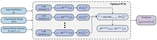
Figure 1.
Iterative Mechanism of OPCK Construction Process.
2.3. Control Equations of Rainfall Infiltration Model
Using the finite element simulation software COMSOL Multiphysics 6.2, an unsaturated slope model was developed to analyze seepage and slope stability during rainfall infiltration. The software provides various contour maps to illustrate the temporal variations in stress field, seepage field, displacement field, and slope Factor of Safety (FOS). MATLAB scripts were used to extract field variable information, thus facilitating the identification of underlying patterns.
2.3.1. Water Flow in Unsaturated Soil
According to Darcy’s Law, the water volume flow rate through a unit area of unsaturated soil can be expressed as follows:
Among them, the unsaturated flow and mechanical deformation are coupled in the last term on the right-hand side of the above equation, where represents the identity matrix and represents the strain rate. It is worth noting that to calculate saturation and pore water pressure, the basic equations of unsaturated flow must be solved. The hydraulic conductivity of unsaturated soil can be expressed as follows:
The initial values of porosity and hydraulic conductivity are denoted by subscripts of zero.
2.3.2. Elastic–Plastic Deformation in Soil
According to Bishop [6], under conditions of constant gas phase and negligible overpressure, the effective stress (σ′) can be expressed as follows:
Under such circumstances, it is assumed that the effective stress parameter (χ) equals saturation. In traditional solid mechanics methods, an additive strain rate decomposition approach is employed to separate the plastic and elastic components of the strain rate, which is based on the continuous tensile plastic relationship correlated with effective stress.
In the formula, represents the strain rate, and represent the plastic and elastic components of the strain rate, respectively, D is the stiffness matrix, and λ is the plastic multiplier. It is worth noting that, in order to represent soil plasticity, the Mohr-Coulomb model is used as the yield criterion, combined with the non-associated flow rule.
2.3.3. Local Safety Factor Method
The Local Safety Factor (LSF) [43] directly evaluates local stability by comparing the shear strength of a point within the slope under potential failure conditions with the current actual shear strength. Its core formula is based on the Mohr-Coulomb criterion as follows:
In the formula, and represent the maximum and minimum effective stresses (kPa), respectively. Combining with the volume averaging method proposed by Wang Xu [44], the regional overall stability can be further quantified through spatial integration.
In the formula, represents the study area; represents the values of different local safety factors within each grid unit of the study area.
2.4. Calculation Procedure
Figure 2 demonstrates the entire process of rainfall-induced slope instability probability analysis presented in this paper. The workflow covers five core steps: parameter modeling, random field generation, surrogate model construction, instability prediction, and result analysis. Detailed explanations are as follows:
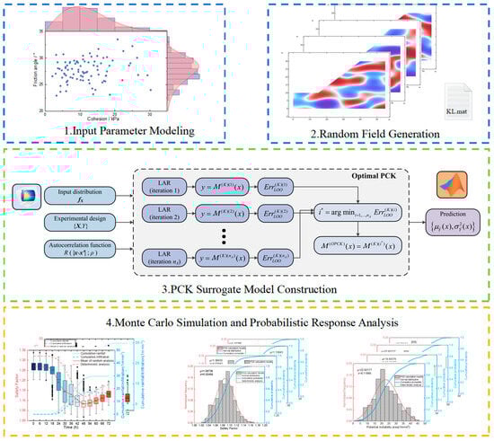
Figure 2.
Numerical Simulation Framework for Uncertainty Analysis.
Step 1: Marginal Distribution Fitting. Firstly, for the physical and mechanical parameters of slope soil, cohesion (C) and internal friction angle (φ) are selected as the main uncertain input variables. Through measured data or literature, marginal probability distribution fitting is performed for these two parameters, and a joint probability density plot (as shown in the upper left of the figure) is used for two-dimensional correlation analysis and visualization modeling, providing basic distribution information for subsequent random field generation.
Step 2: KL Expansion and Spatial Random Field Generation: Based on the aforementioned parameter’s marginal distribution and spatial correlation assumptions, the Karhunen–Loève (KL) expansion method, combined with exponential autocorrelation functions, is used to generate two-dimensional random fields with spatial correlation for cohesion and internal friction angle (as shown in multiple random images in the upper right of the figure). This process achieves high-dimensional dimensionality reduction by truncating KL mode functions, obtaining a set of representative principal component samples (KL modes) to characterize the parameter’s fluctuation characteristics in space.
Step 3: Intelligent Surrogate Model (PCK) Construction: Considering the high time-consuming issue of large-scale finite element/limit equilibrium method calculations, this paper constructs a response surface model based on Latin hypercube sampling (LHS) and PCK (Polynomial Chaos Kriging): First, a certain number of training sample points (input: KL modal parameters, output: safety factor/instability area) are selected, which are calculated through COMSOL finite element simulation. Multiple candidate models are built through stepwise regression (LAR), and the optimal model is selected using cross-validation error (LOO). Finally, the optimal PCK model is output, which can efficiently predict the response mean and variance under any input. This model significantly improves the efficiency of subsequent Monte Carlo sampling.
Step 4: Monte Carlo Simulation and Probabilistic Response Prediction Based on the trained PCK model, the Monte Carlo method is used to generate a large number (e.g., 10,000 groups) of random samples, quickly predicting the safety factor (FS) and potential instability area under each sample. Subsequently, the probability characteristics of all samples are statistically analyzed, and the following are plotted: safety factor box plots at different times; probability distribution of potential instability area; FS/area histograms and cumulative probability curves at critical moments. These results reflect the stability evolution characteristics and uncertain response of the slope during rainfall infiltration.
Step 5: Result Analysis and Risk Identification: Finally, by comparing the deterministic analysis results with the mean/distribution characteristics of stochastic analysis, the limitations of deterministic methods in risk assessment are identified. Meanwhile, combining the evolution trend of safety factors with the spatial distribution pattern of instability areas, the most unstable stage of the system is identified, providing a quantitative basis for early warning window division and protection strategies in slope engineering.
3. Model Settings
This study constructed an idealized two-dimensional slope-platform composite terrain model to simulate and analyze rainfall infiltration and runoff processes. As shown in Figure 3, the model structure mainly consists of an inclined slope and a horizontal platform. The model has a lateral length of 55 m and a longitudinal elevation range from 0 m to 30 m. The slope of the inclined section is 38.23°, and the platform elevation is 10 m. The entire area is divided into regular computational grids for numerical simulation calculations, including 6266 domain units and 431 boundary units.
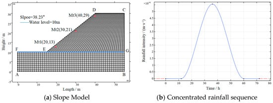
Figure 3.
Slope Geometric Model and Boundary Conditions.
The platform area (left side) extends from point A to F, then to G, and finally to B. The slope area extends from E to D, then to C, and finally to G. Therein, AB serves as the fixed constraint boundary, AF and BC as roller support boundaries, and FEDC as the rainfall boundary. Mt1 (20,13), Mt2 (30,21), and Mt3 (40,29) are selected as typical monitoring points for analyzing the variable change process of the deterministic model. The initial water level is set at 10 m, marked by the blue line in the figure. The rainfall boundary adopts a concentrated rainfall sequence, and the right figure shows the rainfall intensity curve applied to the model. The rainfall duration is approximately 72 h, with a bell-shaped distribution, and the peak rainfall intensity is about 20 mm/h, occurring at the midpoint of the rainfall period (around the 36th hour). Existing research has thoroughly examined extreme rainfall scenarios of constant intensity [45,46] and the bell-shaped rainfall sequence selected for this study is more representative. This rainfall pattern effectively combines ‘prolonged light rainfall’ with ‘short-duration heavy rainfall’: the initial phase of light precipitation serves as a pre-wetting effect, analogous to prolonged light rain conditions; whereas the peak phase in the middle simulates the impact of short-duration heavy rainfall. This non-stationary process elicits a pronounced lag effect in the response of pore water pressure. This rainfall process is used to drive the simulation of the hydrological response in the model, while other hydraulic parameters are shown in the Table 2.
Table 2.
Material Physical and Mechanical Parameters.
4. Result Analysis
4.1. Definitive Analysis
To deeply understand the influence mechanism of rainfall infiltration on slope stability, this section first simulates and analyzes the pore water pressure changes and soil deformation responses of the deterministic model under rainfall conditions. Given known soil parameters, boundary conditions, and rainfall inputs, this model obtains the evolution process of system response through numerical methods, clarifying the combined action characteristics of rainfall on the slope seepage field and stress field.
Figure 4 presents six color-coded images illustrating pore water pressure distribution (in kPa) across six time periods (12 h, 24 h, 36 h, 48 h, 60 h, 72 h). The color gradient from red to blue indicates pressure zones progressing from high to negative. During the initial phase (12–24 h), rainfall has not penetrated deep into the soil, primarily affecting surface layers with minimal pore water pressure changes and predominantly negative pressure. In the intermediate phase (36–48 h), intensified rainfall causes water infiltration into deeper layers, gradually forming positive pressure zones on the upper slope surface. Notably, water accumulation becomes evident at the platform-slope junction, leading to rapid pressure increases. The final phase (60–72 h) shows expanding pore pressure peaks penetrating into the slope interior, with continuously growing saturated zones. This cumulative infiltration effect reflects the potential risk of slope instability.
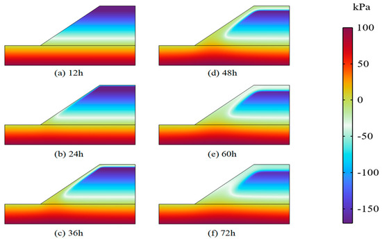
Figure 4.
Evolution process of slope pore water pressure under rainfall conditions.
Figure 5a presents the time-dependent variations in pore water pressure at three monitoring points (Mt1, Mt2, Mt3). Mt1 (near the toe): The pore pressure remains relatively stable with sustained negative pressure, indicating minimal seepage influence in this area. Mt2 (on the slope surface): Pore pressure rapidly increases after 36 h, approaching 0 kPa, suggesting significant water accumulation. Mt3 (near the crest): The fastest pressure rise reaches peak at 48 h before a slight decline, indicating effective drainage commencement after the rainfall peak. Figure 5b shows vertical displacement trends over time: All three points exhibit increasing displacement with prolonged rainfall duration, particularly with rapid displacement growth after 36 h, demonstrating soil softening and sliding caused by infiltration. Mt1 shows maximum displacement: The toe area experiences severe soil saturation and softening, achieving approximately 3.5 mm displacement; Mt2 and Mt3 show delayed displacement. This indicates that the slope surface responds later than the platform and is affected by pore pressure migration. Displacement stabilizes after 48 h, corresponding to the rainfall peak period, suggesting the slope system gradually reaches a new equilibrium state.
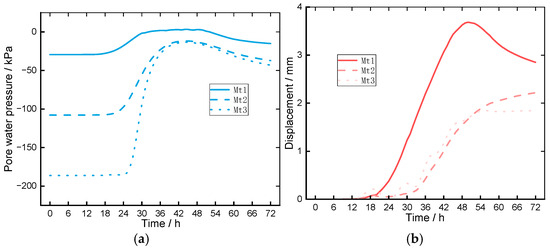
Figure 5.
Variation Curve of Monitoring Points under Rainfall Conditions: (a) Monitoring point pore water pressure variation. (b) Monitoring point displacement variation.
4.2. Uncertainty Analysis
In practical engineering applications, soil physical and mechanical parameters often exhibit significant uncertainties, which may arise from material heterogeneity, measurement errors, or construction disturbances. To better evaluate the impact of these uncertainties on slope responses, this study extends deterministic models by incorporating parameter stochasticity. Specifically, the Karhunen–Loeve (KL) expansion method was applied to generate 1000 sets of stochastic field data for two critical parameters—cohesive force and internal friction angle—thereby enabling comprehensive uncertainty analysis of slope systems.
As shown in the Figure 6, the distribution characteristics of the parameter space were constructed through random sampling of soil parameters—cohesion and friction angle. The scatter plot displays the distribution of samples in the two-dimensional parameter space, while the marginal histogram and kernel density curve reveal that cohesion primarily clusters within the 5–20 kPa range, exhibiting a mildly skewed distribution. The friction angle predominantly falls within the 28–34 range, demonstrating a relatively concentrated distribution. Consequently, this study adopts Weibull-distributed cohesion samples and normally distributed friction angle samples, with their correlation coefficient set at −0.5 [47]. During the construction of the stochastic field, an exponential autocorrelation function was employed to model spatial variability, with horizontal autocorrelation scales set at 15 m and vertical autocorrelation scales at 6 m, reflecting the spatial correlation characteristics of soil parameters in different directions.
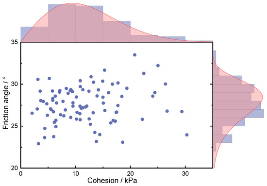
Figure 6.
Sample distribution of cohesion and internal friction angle parameters.
Figure 7 presents a typical spatial distribution sample of soil strength parameters generated by the KL expansion method, including cohesion (Figure 7a) and internal friction angle (Figure 7b). These two diagrams, respectively, demonstrate the spatial variation characteristics of these parameters within the computational domain under spatial correlation control. The figures reveal that the spatial fields exhibit overall continuity and smoothness, aligning with the actual spatial distribution patterns of soil parameters. In Figure 7a’s cohesion spatial field, high-value zones (red) and low-value zones (blue) alternate, primarily concentrated in the lower part of the platform zone and the upper-middle slope area, with maximum values around 15 kPa and minimum values approaching 5 kPa. Figure 7b’s internal friction angle spatial field shows distinct low-friction zones (blue) at the toe of the slope and platform edges, ranging approximately between 25–32 degrees, consistent with the statistical characteristics established earlier.
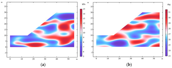
Figure 7.
Random field of shear strength parameters based on Karhunen–Loève expansion method. (a) A typical cohesive force random field. (b) A typical random field of internal friction angle.
Both stochastic fields exhibit significant spatial correlation, with horizontal variations being relatively gradual while vertical fluctuations are more pronounced—a pattern that aligns closely with the predefined autocorrelation scale parameters (15 m horizontally, 6 m vertically). The implementation of such stochastic fields provides a more realistic representation of soil mechanical parameter uncertainties, thereby establishing a reliable input foundation for subsequent probabilistic stability analyses.
To investigate the impact of soil parameter uncertainties on slope stability, this study employs the KL expansion and stochastic field modeling methods to generate 1000 spatially correlated strength parameter samples (cohesion and friction angle) for slope stability analysis. The corresponding safety factors and potential instability areas are calculated using the slope stability model. Considering the cost of large-scale direct simulations, we utilize the PCK surrogate model to train an efficient and reliable surrogate response surface. Subsequently, the trained PCK model generates 10,000 input samples through Monte Carlo sampling, enabling rapid prediction of safety factors and instability areas. The resulting safety factor box plots and multiple response curves at different time points, as shown in Figure 8, comprehensively demonstrate the evolution characteristics of slope stability under uncertainty conditions.
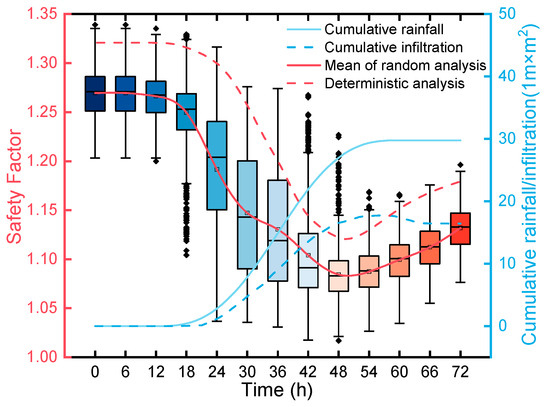
Figure 8.
Box Plot Curves of Safety Factors at Different Time Points.
The box plots in the figure demonstrate the distribution range of safety coefficients at different time intervals (every 6 h), reflecting fluctuations in slope stability caused by parameter uncertainties. During the initial phase (0–24 h, dark blue), the safety coefficients remained consistently high with stable distribution and compact box heights, indicating minimal rainfall impact and good slope stability. In the intermediate phase (24–48 h, light blue to gray), increased rainfall intensity caused a significant drop in average safety coefficients, accompanied by enlarged box heights, extended upper and lower branches, and multiple outliers. This indicates heightened uncertainty in slope response, with some samples entering critical or unstable states. In the later phase (48–72 h, light orange to red), reduced rainfall led to slight convergence of distribution, though the median value remained low, suggesting incomplete recovery to high-stability conditions and persistent risks. The box plots reveal that the safety coefficient fluctuates most dramatically between 36–54 h—coinciding with the peak rainfall infiltration period—highlighting the system’s most unstable and sensitive state during this critical timeframe.
The figure further overlays four key curves that demonstrate the coupling relationship between rainfall processes and stability evolution. The red dashed line (Deterministic analysis) represents deterministic model calculations, showing a steady downward trend but failing to reveal response variability. Notably, the deterministic model significantly overestimates slope stability. The red solid line (mean of random analysis) indicates the mean trajectory of stochastic analysis, aligning closely with the median trend in the box plot and being substantially lower than deterministic results. This suggests traditional analytical methods may overestimate system safety under parameter uncertainties. The blue dashed line (cumulative infiltration) and solid line (cumulative rainfall) represent cumulative infiltration and rainfall, respectively. The sharp decline in the safety factor during the rapid infiltration phase (approximately 30–48 h) indicates a close correlation between slope instability and water infiltration.
In traditional stability analysis, slope safety is typically evaluated using a single safety factor metric, which fails to capture the spatial characteristics of localized instability or progressive failure. To quantify the spatial extent of potential slope instability during rainfall events, this study employs a PCK surrogate model combined with Monte Carlo sampling to analyze the uncertainty of potential instability areas under different time conditions. The surrogate model construction follows the methodology described earlier: First, 1000 spatial correlation intensity parameter samples were generated and integrated with finite element stability analysis results to obtain corresponding instability area data. Subsequently, this dataset was fed into the PCK model for training, generating 10,000 new samples through Monte Carlo simulation to rapidly predict slope instability areas. The resulting box plots and response curves are illustrated in Figure 9.
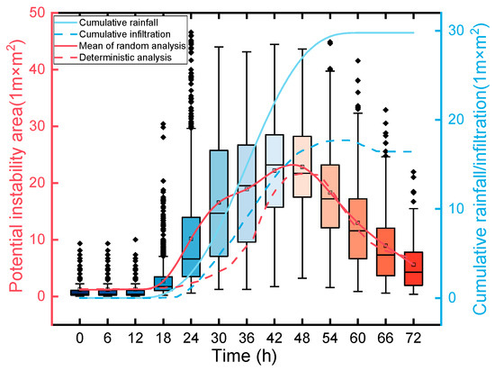
Figure 9.
Box plot curves of potential slope instability areas under different time periods.
The box plot in the figure illustrates the distribution characteristics of potential instability areas under different rainfall periods (measured by the area of regions with local safety coefficients < 1.0). During the initial stage (0–18 h), the instability area is minimal, with the box height approaching zero. Most samples show no instability zones, indicating that rainfall has not yet effectively infiltrated the system, maintaining overall stability. In the development stage (24–48 h), the instability area rapidly expands, the box height significantly increases, and the distribution range fluctuates dramatically. Some samples exhibit instability areas exceeding 40 m2, suggesting the emergence of large potential landslide zones in localized slopes. In the later stage (54–72 h), the instability area shows an overall downward trend as the box scope contracts, though persistent long whiskers and outliers indicate incomplete recovery of instability zones in some samples, revealing lingering spatial instability. Notably, the 36–54 h period coincides with peak instability fluctuations, aligning perfectly with the phase of minimum safety coefficients, further confirming this as the most sensitive and hazardous phase for slope stability.
The red dashed line (Deterministic analysis) depicts the predicted instability area evolution in deterministic analysis, showing a typical peak process with a maximum value of approximately 20 m2, which fails to reflect potential extreme instability scenarios in real-world conditions. The red solid line (Mean of random analysis) represents the mean results of stochastic analysis, exhibiting a trend similar to the deterministic curve but showing significantly higher values during the peak phase (36–54 h). Additionally, the outliers and long whiskers in the box plot reveal that the instability area may expand from zero to dozens of square meters at the same time node, indicating highly uneven risk distribution and complex spatial evolution—critical information that deterministic analysis struggles to capture.
To further investigate the uncertainty characteristics of slope stability response during peak rainfall infiltration periods, this study selected four critical time points (36 h, 42 h, 48 h, and 54 h) for in-depth analysis of the safety factor’s probability distribution. Figure 10 presents the safety factor distribution histogram obtained through the PCK agent model and Monte Carlo sampling, overlaid with normal fitting curves, cumulative probability curves, and deterministic analysis values (dashed line). This visualization reveals the system’s instability trends and risk levels across different phases.
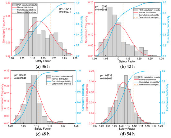
Figure 10.
Probability distribution histogram of slope safety factor during critical rainfall period (36–54 h).
During the initial phase of rapid seepage at 36 h, the safety factor distribution exhibited significant skewness with a mean μ = 1.13043 and standard deviation σ ≈ 0.0597. The frequency distribution showed mild right-skewness with elongated tails, indicating some samples had notably low safety factors. The cumulative probability curve demonstrated a gradual slope, suggesting substantial system response volatility. The deterministic results are positioned to the right of the mean, revealing overestimated risks. This stage marked the initial phase of rapid seepage volume increase, where local slope disturbances began to manifest distinct response asymmetry. At 42 h, when system fluctuations peaked, instability risks intensified with μ = 1.10395 and σ ≈ 0.05038. The distribution became further skewed, with a significant increase in samples below 1.10. The cumulative probability curve rapidly rose near FS = 1.10, indicating a concentration of samples near the critical state. The deterministic values remained above the mean, suggesting underestimated risks. This period represented the system’s most unstable phase, with analysis showing significantly elevated instability probabilities, making it a critical early warning period. At 48 h, system disturbances peaked with a concentrated probability distribution (μ = 1.08435, σ ≈ 0.03042). The distribution converged toward normality, though the mean had dropped near the instability boundary. Reduced standard deviation indicated diminished volatility, signaling the system’s entry into a “global weakening” phase. The deterministic values remained on the right side of the distribution, approximately 5% above the true mean. Despite decreased volatility, overall system stability had fallen below the critical threshold, requiring vigilant monitoring. After 54 h of rainfall, the system partially recovers with a normalized distribution (μ = 1.08738, σ ≈ 0.02468). The distribution remains nearly symmetrical, approaching the standard normal distribution. The cumulative probability curve shows steepness, indicating concentrated system response. The deterministic results align with the mean but show slight rightward skew. During this phase, rainfall intensity diminishes as some areas stabilize, though the system has not fully escaped the critical state.
To further quantify the dynamic fluctuation characteristics of slope spatial response, this section conducts probabilistic statistical analysis on potential instability areas during critical rainfall phases. Figure 11 displays the distribution of instability areas at four time points: 36 h, 42 h, 48 h, and 54 h. The bar chart shows the frequency distribution of simulated samples, with overlaid curves including: the red line representing the normal distribution fit; the blue line indicating the cumulative probability curve; and the yellow dashed line showing deterministic calculation values.
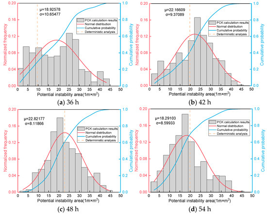
Figure 11.
Probability Distribution Histogram of Potential Slope Instability Area during Critical Rainfall Period (36–54 h).
As shown in Figure 11, the initial response emerges 36 h after rainfall, with a skewed distribution exhibiting significant fluctuations. The mean (μ) is 18.93 m2 and standard deviation (σ) reaches 10.65 m2, representing the highest volatility during this phase. The histogram displays a right-skewed shape with elongated tails, indicating some sample areas exceed 40 m2. The deterministic value (approximately 11 m2) remains notably lower than the mean, failing to identify potential large-scale instability zones. The cumulative probability curve shows slow growth, suggesting inadequate risk identification. Although instability zones have appeared, spatial responses remain highly uncertain, indicating the slope has entered the initial disturbance stage. After 42 h of rainfall infiltration, instability areas expand with enhanced symmetry, achieving a mean of 22.17 m2 and σ = 9.37 m2. The histogram approaches symmetrical distribution, demonstrating good normality fit. Most samples cluster within the 15–30 m2 range, reflecting intensified overall instability trends. The steepening cumulative probability curve indicates concentrated risk in instability areas. The deterministic prediction value (approximately 17 m2) remains below the mean, underscoring insufficient response to extreme scenarios. This phase marks the accelerated expansion period for potential instability development and serves as a critical window for risk management. At 48 h post-rainfall infiltration, the system reaches its most unstable phase with concentrated risks. The distribution shows reduced volatility (μ = 22.82 m2, σ = 8.12 m2) and closer convergence to normality. The deterministic value stabilizes at approximately 20 m2, though tail risks remain underrepresented. Cumulative probability shifts concentrate, with 60% of samples falling within the 15–30 m2 range. This stage marks the peak plateau of instability areas, where most samples exhibit large unstable zones, constituting the critical period for emergency response. By 54 h, rainfall intensity diminishes, and instability scope narrows (μ = 18.29 m2, σ = 8.60 m2). The distribution shifts rightward with extended tails, showing occasional large-scale instability cases. While the mean value decreases, volatility persists, indicating partial regional instability. The deterministic value again underestimates extreme responses. The system begins recovery, but local high-risk areas—particularly tail samples—remain critical for monitoring extreme scenarios.
5. Discussion
5.1. Sensitivity Analysis of KL Expansion Truncation Order
The accuracy and computational efficiency of the random field discretization are critically dependent on the truncation order M in the KL expansion. A low M may fail to capture the local variability of soil properties, leading to an underestimation of failure probability, while an excessively high M increases computational cost without significant accuracy gains. To address the sensitivity of the simulation results to the truncation order, we conducted a convergence analysis of the global variance error and the cumulative energy contribution.
Figure 12 illustrates the impact of the truncation order M on the stochastic field representation accuracy. The blue curve represents the average variance error (defined as ), while the red curve depicts the cumulative contribution of eigenvalues.
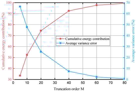
Figure 12.
Impact of the truncation order M on the stochastic field representation accuracy.
As observed in Figure 12, the variance error exhibits a sharp decline as M increases from 5 to 80. Specifically:
At M = 5, the representation is poor, with a variance error exceeding 65% and a cumulative energy contribution of less than 35%. This indicates that low-order truncation results in a significant loss of high-frequency fluctuation information. As M reaches 40, the variance error drops significantly to approximately 8%, and the cumulative energy contribution surpasses 90%. The curve begins to flatten, suggesting that the marginal gain from adding more terms diminishes. When M increases to 60 and 80, the cumulative energy contribution exceeds 97.7% and approaches 99%, respectively, while the variance error becomes negligible (<3%).
Considering the balance between numerical precision and computational efficiency, a truncation order of M = 50 (corresponding to a cumulative energy threshold of approximately 95%) was selected for the uncertainty analysis. This threshold ensures that the generated random fields retain sufficient spatial variability features required for slope stability assessment, while maintaining a manageable dimensionality for the stochastic finite element model.
5.2. Comparison of Surrogate Model Performance
This section compares the predictive capabilities of PCE, Kriging, and PCK models based on the coefficient of determination (R2), Root Mean Square Error (RMSE), and construction time. The parity plots comparing the predicted and true Factor of Safety (FS) are presented in Figure 13.
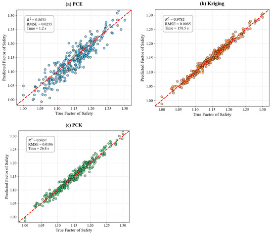
Figure 13.
Prediction performance diagrams for three distinct proxy models.
The PCE model (Figure 13a) shows the lowest accuracy (R2 = 0.8031, RMSE = 0.0255) with noticeable scatter, although it is the most computationally efficient (1.2 s). Conversely, the Kriging model (Figure 13b) yields the highest precision (R2 = 0.9782, RMSE = 0.0085), but this comes at the expense of the highest computational cost (158.5 s).
The PCK model (Figure 13c) demonstrates a superior balance between accuracy and efficiency. By combining the global trend capture of PCE with the local refinement of Kriging, PCK achieves an accuracy (R2 = 0.9657, RMSE = 0.0106) close to that of the Kriging model. Notably, its computational time is drastically reduced to 26.8 s, which is approximately six times faster than the pure Kriging approach. Given these results, the PCK model is deemed the most robust and efficient surrogate for the probabilistic analysis.
5.3. Monte Carlo Simulation Convergence
To assess the accuracy of the surrogate models proposed in this study, a direct Monte Carlo Simulation (MCS) was employed as the benchmark solution. The reliability of the MCS results depends heavily on the sample size; an insufficient number of simulations may lead to unconverged statistical moments. Therefore, a convergence analysis was conducted to determine the appropriate number of realizations.
Figure 14 illustrates the convergence history of the cumulative mean safety factor with respect to the number of simulations. As observed in the figure, the cumulative mean exhibits significant fluctuations during the initial phase (0 to 2000 simulations) due to the randomness of the sampling process. However, as the number of simulations increases, the curve gradually stabilizes. Beyond 6000 simulations, the variation becomes negligible, and the mean value converges asymptotically to approximately 1.140.
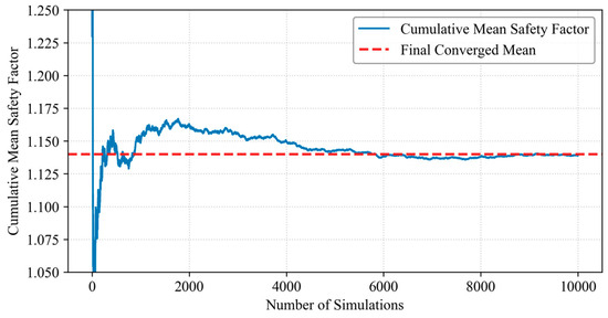
Figure 14.
Convergence history of the Monte Carlo Simulation.
Consequently, a sample size of N = 10,000 was selected for the benchmark dataset. This quantity ensures that the statistical error is minimized, providing a robust “ground truth” for evaluating the performance of the PCE, Kriging, and PCK models.
6. Conclusions
This study addresses slope instability caused by rainfall infiltration, focusing on key scientific challenges including soil parameter uncertainties, seepage–mechanical coupling responses, and probabilistic risk evolution. It develops an integrated slope instability analysis framework combining random field modeling, agent-based modeling, and probabilistic simulation. The key findings are as follows:
(1) The Karhunen–Loeve (KL) expansion method effectively constructs spatially correlated soil strength parameter fields by fitting the edge distributions of cohesion and internal friction angle. By combining the KL expansion with exponential autocorrelation functions, a two-dimensional spatially correlated parameter random field is generated. This field demonstrates distinct spatial correlation and fluctuation patterns, accurately capturing the heterogeneity of soil physical parameters across different regions, thereby providing reliable input for subsequent analyses.
(2) The Polynomial Chaos Kriging (PCK) surrogate model combines global and local approximation capabilities, delivering both high accuracy and computational efficiency. This study introduces a PCK model that integrates the global expansion advantages of Polynomial Chaos Expansion (PCE) with the local interpolation capabilities of Kriging. By employing the LARS algorithm to select the optimal polynomial set and using leave-one-out cross-validation (LOO-CV) to optimize the model structure, we ultimately obtain a high-precision, low-error optimal PCK model. Compared to traditional finite element methods, PCK maintains response accuracy while improving computational efficiency by several dozen times, significantly reducing the cost of large-scale sample simulations.
(3) Uncertainty simulations revealed critical phases and spatial risk characteristics in slope stability evolution. Monte Carlo simulations demonstrated that both the slope safety factor and potential instability area exhibited distinct temporal patterns during rainfall events. The 36–54 h period proved to be the most critical unstable phase, characterized by rapid intensification of rainfall infiltration, significant pore pressure increases, and dramatic fluctuations in slope response, making the system highly sensitive. During this phase, the safety factor reached its lowest average value with maximum standard deviation, while potential instability areas showed significant volatility. Some samples even exhibited large-scale sliding zones, highlighting pronounced spatiotemporal uncertainties.
(4) Traditional deterministic methods systematically overestimate risks and fail to reveal extreme responses. Comparative analysis shows that the safety factors and instability areas calculated by conventional deterministic models are consistently higher than the stochastic averages predicted by the PCK model, failing to accurately reflect the risk expansion caused by uncertainties. Moreover, deterministic analysis cannot identify extreme instability scenarios in tail samples, which may underestimate warning ranges and protective requirements, potentially creating safety blind spots in actual engineering projects.
Author Contributions
Conceptualization, B.Z.; Methodology, B.Z., K.H., H.S. and Q.C.; Software, B.Z. and Q.C.; Validation, B.Z.; Formal Analysis, B.Z., Q.C. and H.W.; Investigation, B.Z. and Q.C.; Resources, B.Z.; Data Curation, H.W.; Writing—Original Draft Preparation, B.Z.; Writing—Review & Editing, B.Z., K.H. and H.S.; Visualization, B.Z. and Q.C.; Supervision, K.H. and H.S.; Project Administration, B.Z. All authors have read and agreed to the published version of the manuscript.
Funding
This research received no external funding.
Data Availability Statement
The original contributions presented in this study are included in the article. Further inquiries can be directed to the corresponding author.
Conflicts of Interest
The authors declare no conflicts of interest.
References
- Gariano, L.S.; Guzzetti, F. Landslides in a changing climate. Earth-Sci. Rev. 2016, 162, 227–252. [Google Scholar] [CrossRef]
- Harianto, R.; Alfrendo, S.; Choon, E.L. Effects of Rainfall Characteristics on the Stability of Tropical Residual Soil Slope. In Proceedings of the E3S Web of Conferences, Lyon, France, 17–21 October 2016; p. 915004. [Google Scholar] [CrossRef]
- Ministry of Natural Resources of the People’s Republic of China. 2022 China Natural Resources Statistical Bulletin (Excerpts). China Natural Resources News, 13 April 2023; (In Chinese). [Google Scholar] [CrossRef]
- Jia, Z.; Zhu, L.; Guo, M.; Zhang, Y.; Zhang, X.; Yin, Y. Rainfall-Induced Failure Mechanisms of Cohesive Slopes in Deep Excavations. Geotech. Geol. Eng. 2025, 43, 495. [Google Scholar] [CrossRef]
- Wang, X.; Zhang, Y.; Li, W.; Xiao, J.; Tan, F.; Huang, C. Mechanisms of pile-soil stress and deformation in excavations under the coupled effects of excavation disturbance and extreme rainfall infiltration. Sci. Rep. 2025. [Google Scholar] [CrossRef] [PubMed]
- Bishop, A.W. The Use of the Slip Circle in the Stability Analysis of Slopes. Géotechnique 1955, 5, 7–17. [Google Scholar] [CrossRef]
- Janbu, N. Slope Stability Computations; Embankment Dam Engineering Casagrande Volume; John Wiley & Sons, Inc.: New York, NY, USA, 1973. [Google Scholar]
- Morgenstern, N.R.; Price, V.E. The Analysis of the Stability of General Slip Surfaces. Géotechnique 1965, 15, 79–93. [Google Scholar] [CrossRef]
- Tozato, K.; Dolojan, N.L.J.; Touge, Y.; Kure, S.; Moriguchi, S.; Kawagoe, S.; Kazama, S.; Terada, K. Limit equilibrium method-based 3D slope stability analysis for wide area considering influence of rainfall. Eng. Geol. 2022, 308, 106808. [Google Scholar] [CrossRef]
- Wang, R.; Guo, R.; Liu, C. Study on Hybrid Stress Finite Elements of 3D Arbitrary Polyhedral Considering Gravity. Acta Mech. Solida Sin. 2025, 1–11. [Google Scholar] [CrossRef]
- Karl, T. Stability of Steep Slopes on Hard Unweathered Rock. Geotechnique 1962, 12, 251–270. [Google Scholar] [CrossRef]
- Metya, S.; Bhattacharya, G. Probabilistic Stability Analysis of the Bois Brule Levee Considering the Effect of Spatial Variability of Soil Properties Based on a New Discretization Model. Indian Geotech. J. 2016, 46, 152–163. [Google Scholar] [CrossRef]
- Griffiths, D.V.; Lane, P.A. Slope stability analysis by finite elements. Géotechnique 2001, 51, 653–654. [Google Scholar] [CrossRef]
- Peng, X.; Li, D.Q.; Cao, Z.J.; Tang, X.S.; Zhou, C.B. Monte Carlo simulation-based reliability design method for rock slopes. J. Rock Mech. Eng. 2016, 35, 3794–3804. (In Chinese) [Google Scholar]
- Tamimi, S.; Amadei, B.; Frangopol, D.M. Monte Carlo simulation of rock slope reliability. Comput. Struct. 1989, 33, 1495–1505. [Google Scholar] [CrossRef]
- Pascual, B.; Adhikari, S. A reduced polynomial chaos expansion method for the stochastic finite element analysis. Sadhana Acad. Proc. Eng. Sci. 2012, 37, 319–340. [Google Scholar] [CrossRef]
- Wong, F.S. Slope Reliability and Response Surface Method. J. Geotech. Eng. Asce 1985, 111, 32–53. [Google Scholar] [CrossRef]
- Cheng, Q.; Cheng, Z. Global Sensitivity Analysis of Structural Random Response Based on Polynomial Chaotic Expansion. Acad. J. Sci. Technol. 2025, 16, 78–80. [Google Scholar] [CrossRef]
- De Meulenaere, R.; Coppitters, D.; Sikkema, A.; Maertens, T.; Blondeau, J. Uncertainty Quantification for Thermodynamic Simulations with High-Dimensional Input Spaces Using Sparse Polynomial Chaos Expansion: Retrofit of a Large Thermal Power Plant. Appl. Sci. 2023, 13, 10751. [Google Scholar] [CrossRef]
- Vanmarcke, J.H. Random Fields: Analysis and Synthesis; MIT Press: Cambridge, MA, USA, 1983; Available online: https://books.google.com.sg/books?hl=zh-CN&lr=&id=0MCxDV1bonAC&oi=fnd&pg=PR5&ots=LPdjpB2kSS&sig=3YdvFv-xnQRsWuUGRe3sZt-aSCI&redir_esc=y#v=onepage&q&f=false (accessed on 15 November 2025).
- Wolfe, G.F.D.; Griffiths, D.V.; Huang, J. Probabilistic Slope Stability Analysis Of Embankment Dams Using Random Finite Elements (Rfem). In Proceedings of the Association of State Dam Safety Officials Annual Conference, Washington, DC, USA, 20–23 September 2010. [Google Scholar]
- Li, J.; Spencer, B.F.; Elnashai, A.S. Bayesian Updating of Fragility Functions using Hybrid Simulation. J. Struct. Eng. 2013, 139, 1160–1171. Available online: https://www.researchgate.net/publication/261987177_Bayesian_Updating_of_Fragility_Functions_Using_Hybrid_Simulation (accessed on 15 November 2025). [CrossRef]
- Griffiths, D.V.; Fentont, G.A. The Random Finite Element Method (RFEM) in Steady Seepage Analysis; Springer: Vienna, Austria, 2007. [Google Scholar] [CrossRef]
- Tozato, K.; Sugo, D.; Dolojan, N.L.J.; Nomura, R.; Terada, K.; Takase, S.; Kaneko, K.; Moriguchi, S. Rapid prediction of rainfall-induced landslides over a wide area aided by a simulation-based surrogate model. Comput. Geotech. 2025, 188, 107480. [Google Scholar] [CrossRef]
- Keshtegar, B.; Hasanipanah, M.; Nguyen-Thoi, T.; Yagiz, S.; Amnieh, H.B. Potential efficacy and application of a new statistical meta based-model to predict TBM performance. Int. J. Min. Reclam. Environ. 2021, 35, 471–487. [Google Scholar] [CrossRef]
- Shibata, T.; Koch, M.C.; Papaioannou, I.; Fujisawa, K. Efficient Bayesian inversion for simultaneous estimation of geometry and spatial field using the Karhunen-Loève expansion. Comput. Methods Appl. Mech. Eng. 2025, 441, 117960. [Google Scholar] [CrossRef]
- Yin, Z.; Pan, W.; Zheng, X. A spectral-fast Voronoi framework based on multivariate Karhunen–Loève expansion for simulation of two-dimensional random fields. Appl. Math. Model. 2026, 150, 116422. [Google Scholar] [CrossRef]
- Wu, Y.; Zhi, P. Reliability assessment of RAC chloride concentration using Karhunen–Loève expansion with digital-image kernels. Constr. Build. Mater. 2020, 245, 118352. [Google Scholar] [CrossRef]
- Zhou, B.; Li, R.; Zhang, C.-S.; Chen, Z. Combined discontinuous and continuous Galerkin methods for fractured poroelastic media flow on polytopic grids. J. Comput. Appl. Math. 2026, 474, 116986. [Google Scholar] [CrossRef]
- Ahmed, Q.M.; Salahuddin, A.A. A polynomial extrapolation-based wavelet-Galerkin method for dynamic response reconstruction. Ain Shams Eng. J. 2023, 14, 102009. [Google Scholar]
- Blatman, G.; Sudret, B. Adaptive sparse polynomial chaos expansion based on least angle regression. J. Comput. Phys. 2011, 230, 2345–2367. [Google Scholar] [CrossRef]
- Chowdhury, R.; Rao, B. Assessment of high dimensional model representation techniques for reliability analysis. Probab. Eng. Mech. 2009, 24, 100–115. [Google Scholar] [CrossRef]
- Shen, W.; Lin, J.K.D.; Chang, C. Design and analysis of computer experiment via dimensional analysis. Qual. Eng. 2018, 30, 311–328. [Google Scholar] [CrossRef]
- Sudret, B. Global sensitivity analysis using polynomial chaos expansions. Reliab. Eng. Syst. Saf. 2008, 93, 964–979. [Google Scholar] [CrossRef]
- Ghanem, R.G.; Spanos, P.D. Stochastic Finite Elements: A Spectral Approach; Courier Corporation: Chelmsford, MA, USA, 2003. [Google Scholar]
- Xu, J.; Wang, D. Structural reliability analysis based on polynomial chaos, Voronoi cells and dimension reduction technique. Reliab. Eng. Syst. Saf. 2019, 185, 329–340. [Google Scholar] [CrossRef]
- Marelli, L.N.; Sudret, S.B. UQLab User Manual–Polynomial Chaos Expansions; Technical Report; Report UQLab-V1.4-104; Chair of Risk, Safety and Uncertainty Quantification; ETH: Zurich, Switzerland, 2021. [Google Scholar]
- Babacan, S.D.; Molina, R.; Katsaggelos, A.K. Bayesian compressive sensingusing Laplace priors. IEEE Trans. Image Process. 2009, 19, 53–63. [Google Scholar] [CrossRef]
- Lataniotis, C.; Wicaksono, D.; Marelli, S.; Sudret, B. UQLab User Manual–Kriging (Gaussian Process Modeling); Technical Report; Report UQLab-V1.3-105; Chair of Risk, Safety and Uncertainty Quantification; ETH: Zurich, Switzerland, 2019. [Google Scholar]
- Pan, Q.-J.; Zhang, R.-F.; Ye, X.-Y.; Li, Z.-W. An efficient method combining polynomial-chaos kriging and adaptive radial-based importance sampling for reliability analysis. Comput. Geotech. 2021, 140, 104434. [Google Scholar] [CrossRef]
- Schöbi, R. Surrogate models for uncertainty quantification in the contextof imprecise probability modelling. In IBK Bericht; ETH: Zurich, Switzerland, 2019; p. 505. [Google Scholar]
- van Genuchten, M.T. A closed-form equation for predicting the hydraulic conductivity of unsaturated soils. Soil Sci. Soc. Am. J. 1980, 44, 892–898. [Google Scholar] [CrossRef]
- Lu, N.; Şener-Kaya, B.; Wayllace, A.; Godt, J.W. Analysis of rainfall-induced slope instability using a field of local factor of safety. Water Resour. Res. 2012, 48, 9524. [Google Scholar] [CrossRef]
- Xu, W. Impact of Slope Runoff on Shallow Slope Stability; Zhejiang University: Hangzhou, China, 2023. (In Chinese) [Google Scholar]
- Nian, G.; Chen, Z.; Zhang, L.; Bao, M.; Zhou, Z. Treatment and application of two boundary conditions in slope rainfall infiltration. Rock. Soil Mech. 2020, 41, 4105–4115. (In Chinese) [Google Scholar] [CrossRef]
- Nian, G.; Chen, Z.; Zhou, Z.; Zhang, L.; Bao, M. Seepage and stability analysis of fractured rock slopes based on the dual-medium model. J. Coal Sci. 2020, 45, 736–746. (In Chinese) [Google Scholar] [CrossRef]
- Zhou, X. Copula-Based Simulation of Cross-Correlation Stochastic Fields and Reliability Analysis of Soil Slopes. Ph.D. Thesis, Wuhan University of Technology, Wuhan, China, 2020. (In Chinese). [Google Scholar] [CrossRef]


Disclaimer/Publisher’s Note: The statements, opinions and data contained in all publications are solely those of the individual author(s) and contributor(s) and not of MDPI and/or the editor(s). MDPI and/or the editor(s) disclaim responsibility for any injury to people or property resulting from any ideas, methods, instructions or products referred to in the content. |
© 2026 by the authors. Licensee MDPI, Basel, Switzerland. This article is an open access article distributed under the terms and conditions of the Creative Commons Attribution (CC BY) license.