Review

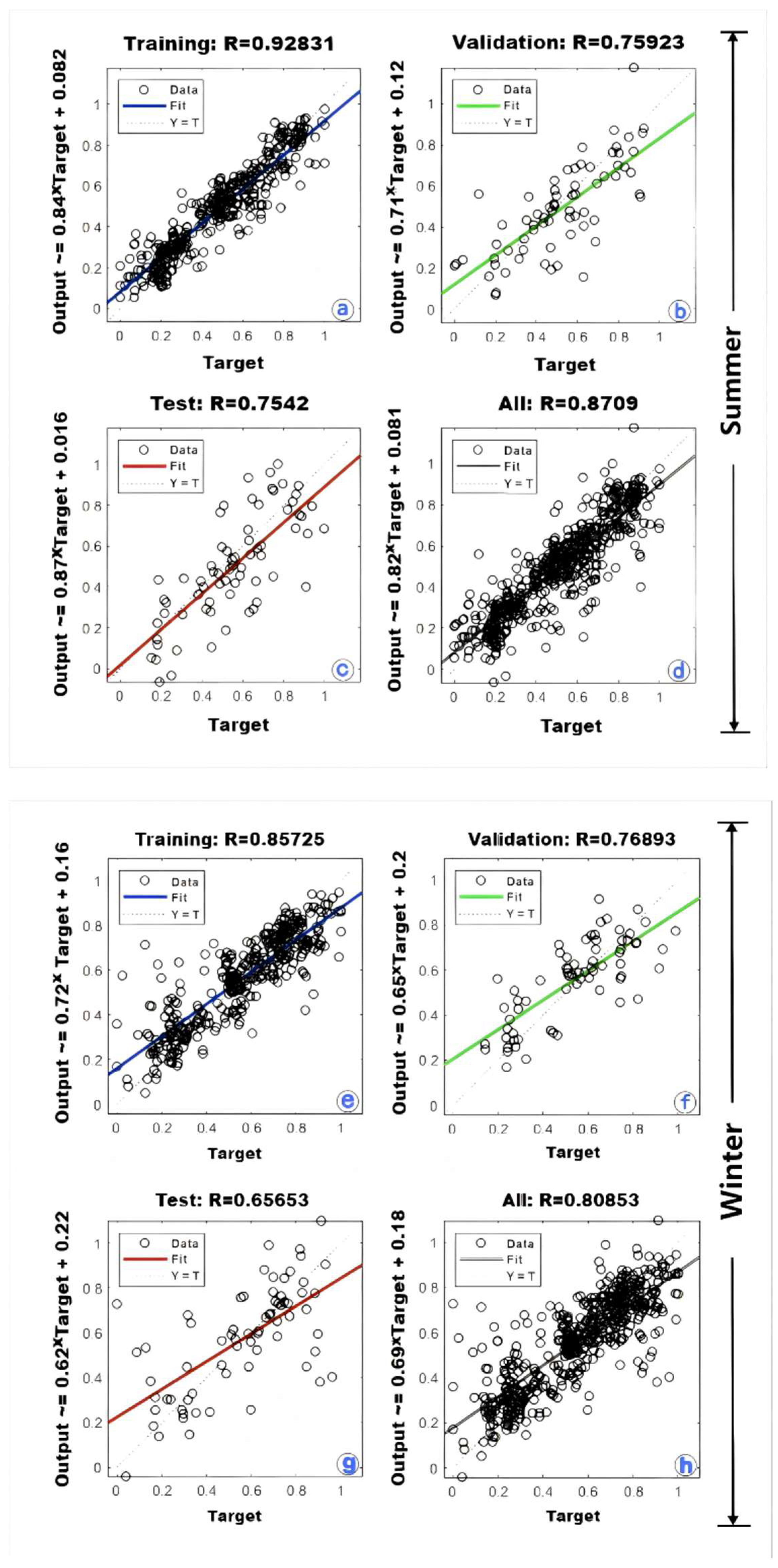
An Overview of the Indian Monsoon Using Micropaleontological, Geochemical, and Artificial Neural Network (ANN) Proxies During the Late Quaternary

1
School of Oceanography and Ecological Science, Shanghai Ocean University, Shanghai 201306, China
2
International Research Center for Marine Biosciences, Shanghai Ocean University, Ministry of Science and Technology, Shanghai 201306, China
3
Department of Earth and Environmental Sciences, University of Ottawa, Ottawa, ON K1N 6N5, Canada
4
School of Earth Sciences, Ohio State University, Columbus, OH 43201, USA
5
College of Life Sciences, Jiangxi Science and Technology Normal University, Nanchang 330038, China
*
Author to whom correspondence should be addressed.
Geosciences 2025, 15(7), 241; https://doi.org/10.3390/geosciences15070241
Submission received: 2 February 2025 / Revised: 29 May 2025 / Accepted: 20 June 2025 / Published: 24 June 2025
(This article belongs to the Section Climate and Environment)

Abstract

Atmospheric pressure gradients determine the dynamics of the southwest monsoon (SWM) and northeast monsoon (NEM), resulting in rainfall in the Indian subcontinent. Consequently, the surface salinity, mixed layer, and thermocline are impacted by the seasonal freshwater outflow and direct rainfall. Moreover, seasonally reversing monsoon gyre and associated currents govern the northern Indian Ocean surface oceanography. This study provides an overview of the impact of these dynamic changes on sea surface temperature, salinity, and productivity by integrating more than 3000 planktonic foraminiferal censuses and bulk sediment geochemical data from sediment core tops, plankton tows, and nets between 25° N and 10° S and 40° E and 110° E of the past six decades. These data were used to construct spatial maps of the five most dominant planktonic foraminifers and illuminate their underlying environmental factors. Moreover, the cured foraminiferal censuses and the modern oceanographic data were used to test the newly developed artificial neural network (ANN) algorithm to calculate the relationship with modern water column temperatures (WCTs). Furthermore, the tested relationship between the ANN derived models was applied to two foraminiferal censuses from the northern Bay of Bengal core MGS29-GC02 (13°31′59″ N; 91°48′21″ E) and the southern Bay of Bengal Ocean Drilling Program (ODP) Site 758 (5°23.05′ N; 90°21.67′ E) to reconstruct the WCTs of the past 890 ka. The reconstructed WCTs at the 10 m water depth of core GC02 suggest dramatic changes in the sea surface during the deglacial periods (i.e., Bolling–Allerǿd and Younger Dryas) compared to the Holocene. The WCTs at Site 758 indicate a shift in the mixed-layer summer temperature during the past 890 ka at the ODP Site, in which the post-Mid-Brunhes period (at 425 ka) was overall warmer than during the prior time. However, the regional alkenone-derived sea-surface temperatures (SSTs) do not show such a shift in the mixed layer. Therefore, this study hypothesizes that the divergence in regional SSTs is most likely due to differences in seasonality and depth habitats in the paleo-proxies.

1. Introduction

One of the dramatic changes in tropical hydrology and its ensuing impact on the Indian subcontinent is the regular return of the Indian summer monsoon (ISM), also known as the southwest monsoon (SWM). It forms due to seasonal differences in solar insolation (heating), resulting in a thermal and atmospheric pressure gradient between the adjacent continental landmasses (mostly the Tibetan Plateau) and the southern Indian Ocean (at about 30° S) [1,2]. Ensemble model data [3] indicate that the south Indian Ocean contributes the most summer season moisture to India, representing 46%, followed by local recycling (30.40%), the Arabian Sea (19.6%), and the Bay of Bengal (4%). More recent investigations indicate an even greater role of synoptic lows and depressions, accounting for 60 to 80% of the total precipitation in the core monsoon zone [4] and up to 80% of total Indian precipitation [5]. In any event, this synoptic low pressure sets the stage for a strong low-level cross-equatorial airflow, which reaches its maximum intensity during the SWM. It directly affects the agrarian lives of millions of people [6] in the Indian subcontinent. Paleo-proxy records show that the SWM strength switched between weak and strong states on the centennial to millennial scale [7,8], impacting the rainfall in the Ganga–Brahmaputra–Meghna (GBM) catchment. In contrast to the SWM, the less prominent northeast winter monsoon (NEM) winds reverse, with cold, dry air blowing from the atmospheric high-pressure area in Siberia toward the ocean. As a result, the Bay of Bengal, Andaman Sea, and Arabian Sea receive an insignificant runoff from the Indian rivers compared to the SWM.
The Bay of Bengal (BoB), surrounded on three sides by land, is the world’s least saline ocean basin and receives ~2950 km3 of runoff annually [9]. The BoB precipitation begins between late April and mid-May, reaching ~10° N between mid-May and mid-June, with strong rainfall over the northern BoB and India from June to September [10]. The entire system is strongly seasonal (Figure 1), with 80 to 90% of precipitation resulting from the SWM (June to September) [11]. Evaporation plays a minor role, with precipitation plus runoff minus evaporation [(P + R) − E] being positive throughout the year [12]. Runoff to the BoB is dominated by GBM discharge, peaking at ~1 × 10⁵ m3/s between August and September, approximately a month after peak precipitation over the surrounding landmasses in July [13]. Hence, the BoB surface salinity is strongly coupled to the precipitation and runoff (Figure 1 and Figure 2).
In contrast to the BoB, two seaways, namely, the straits of Bab-el-Mandeb and Hormuz, connect the Red Sea and the Persian Gulf, respectively, to the north, providing conduits for high salinity waters to the Arabian Sea during the summer (Figure 1). The Persian Gulf is separated from the northern Indian Ocean by a 25 m shallow bathymetric constriction, whereas the sill depth of the Red Sea is 137 m. On the eastern margin, there are minor discharges from a few small Indian rivers, except the Indus River, with a 54 km3 annual discharge. The other notable feature on the Somalia and Oman margins in the western Arabian Sea during the SWM is the intense upwelling driven by Ekman transport, which brings cold, nutrient-rich deep water to the surface, thereby enhancing productivity [14,15] and cooling the sea surface. In contrast to the Somali and Oman margin, a weak upwelling system on the west coast of India (e.g., Pakistan margin) during the NEM seems to be mostly restricted to shelf waters [16]. One of the physical demonstrations of the upwelling system is the seasonal appearance of the oxygen minimum zone (OMZ) along the margins of Somalia, Oman, and Pakistan. However, the extent to which the OMZ determines the preservation of planktonic foraminifera and the accumulation of organic carbon on these margins has not been fully explored.
Figure 1. The approximate position of various Indian subcontinent rivers and surface currents of the northern Indian Ocean and the location of sediment cores discussed in this study are shown. The red and blue arrows illustrate presumed moisture pathways during the summer (SWM) and winter (NEM) Indian monsoons. Black and white arrows show various surface currents that reverse directions between SWM and NEM, mostly in the tropical and northern Indian Ocean [17]. The large circles covering the Arabian Sea and Bay of Bengal reflect evaporation and precipitation [18]. Note: EICC and WICC, East and West Indian Coastal Currents; NMC/SMC, NE, and SW Monsoon Currents; NEC, North Equatorial Current; SEC, South Equatorial Current; EACC, East African Coastal Current; the summer equivalent of SECC is located further south, south of 10° S (see [19]. Note also that IR = Indus River, GR = Ganga River, BR = Brahmaputra River, MR = Meghna River, IrR = Irrawaddy River, SR = Salween River, BoB = Bay of Bengal, and AS = Andaman Sea.
Geosciences 15 00241 g001
A stronger SWM greatly increases precipitation over the GBM catchments, leading to enhanced runoff and direct rainfall over the BoB, resulting in low salinity (~24 psu; practical salinity unit) and a freshwater lid during June. However, the highest annual salinity (34 psu) in the BoB occurs in May (Figure 2). This salinity difference of ~10 psu reduces to ~2 psu in the autumn/winter [20] when the inter-tropical convergence zone retreats toward the equator, the GBM runoff decreases, and direct rainfall ceases [10]. These low-salinity waters flow along the East India Coastal Current on the eastern Indian continental margin, which reverses after the SWM. The second hydrologic cycle tied to the migration of the SWM is the Irrawaddy outflow draining into the Andaman Sea. Consequently, the low-salinity freshwater plume begins to emerge in the Andaman Sea from the end of summer to late fall (Figure 2f). In contrast to the BoB, the Arabian Sea is mostly influenced by atmospheric net positive divergence flux during the summer (E-P; 3 to 3.5 mm/day [18], hence inducing more evaporation (green circle, Figure 1). As a result, paleo-proxy records [18] from the Arabian Sea region cover an important but incomplete picture of the SWM. In comparison, atmospheric net negative divergence and GBM-Irrawaddy outflow dominate the BoB (blue circle, Figure 1). Despite the importance of understanding the impact of past rainfall intensity and, consequently, the GBM-Irrawaddy runoff into the BoB, very few fragmentary paleo-proxy records exist that cover the last glacial period (the past 25 ka); thus, long-term perspectives on the SWM are scarce.
Figure 2. Sea-surface salinity (SSS) and sea-surface temperature (SST) of the northern Indian Ocean are between 40° E and 100° E and 10° S and 35° N. Striking salinity conditions developed between the Arabian Sea and the Bay of Bengal during the (a) NEM and (b) SWM, in which the highest salinity was observed in the northeastern Arabian Sea. A low-salinity cone was observed in the Bay of Bengal during the NEM (a). Due to the low GBM discharge, a large low-salinity gradient (from North to South) was found during the SWM, resulting from the combined effect of the GBM discharge and direct precipitation. There is no difference in temperature in the Arabian Sea and Bay of Bengal thermocline during the NEM (c), but a distinct difference appears during the SWM (d). A well-developed salinity cell with 36.5 psu (e) was found in the Arabian Sea during the NEM. However, two distinct low-salinity cells were discovered around the southern tip of the Indian subcontinent. In contrast to the NEM, the entire Arabian Sea shows high salinity, but low salinity (f) in the Bay of Bengal, demonstrating the salinity gradient between the two basins due to the ISM. Data used to derive these maps were obtained from Reagan et al. [20] and Locarnini et al. [21], and the Ocean Data View program was used to plot salinity and temperature.
Geosciences 15 00241 g002
The understanding of the long-term ISM evolution, due to the close connection between the solid Earth and global atmospheric circulation since the rise of the Himalayas [22], has been of great scientific interest. The rise of the Himalayas has also been partially attributed to changes in the global biogeochemical cycles, including the Earth’s regulation of atmospheric CO2 concentration [23]. Moreover, considering the population density of the Indian subcontinent and its surrounding regions, as well as their dependence on rainfall for subsistence farming, understanding the dynamics of the ISM is of great societal significance. Due to low sedimentation rates in the depositional environment in the northern Indian Ocean, the traditional piston cores provide mostly short-term climate history. To unravel a longer-term perspective on the ISM, the Deep-Sea Drilling Program (DSDP) and Ocean Drilling Program (ODP) drilled numerous sites between 1972 and 1987 in the BoB and the Arabian Sea. The newest drilling campaigns by the International Ocean Drilling Program (IODP) between 2013 and 2023, designated “marginal seas around Asia,” drilled four sites in the BoB and the eastern Arabian Sea [24]. These ongoing efforts by the international scientific community reflect a desire to better understand the dynamics of the ISM and their impact on global biogeochemical cycles and regional hydrology.
Planktonic foraminifera have been used over the last six decades as qualitative to semi-quantitative indicators of past sea-surface temperature (SST), water mass dynamics, and oceanographic fronts in the North Atlantic and Indian oceans [25,26,27,28,29]. Imbrie and Kipp [30] used the foraminiferal census to develop a transfer function to estimate SST in the North Atlantic, which Kipp [31] updated by adding additional core top data. Hutson and Prell [32] reported a paleontological transfer function for Indian Ocean planktonic foraminifera. The Climate Long-Range Investigation, Mapping, and Prediction (CLIMAP Project (refs. [33,34]) used foraminiferal assemblages census to reconstruct SST during the Last Glacial Maximum (LGM). Prell and the Brown University group [35] provided the first foraminiferal distribution and their use in reconstructing the SST during the LGM and the last glacial cycle from the Indian Ocean. Prell et al. [36] reconstructed the surface circulation of the Indian Ocean during the 18 ka, whereas Cullen [37] used sediment cores between the equator and 20° N covering mostly the BoB to reconstruct past salinity through foraminiferal census for the same period. Subsequently, Cullen and Prell [38] used >250 surface sediment samples between 12° S and 25° N of the Indian Ocean, providing a history of the distribution and preservation of planktonic foraminifera. Using sediments from the Oman margin ODP Site 723, Anderson and Prell [39] reported foraminiferal census, especially the % Globigerina bulloides, to assess the SWM of the past 300 ka. However, the authors did not use a foraminiferal census to reconstruct sea surface temperatures (SST). Moreover, Vénce-Peyré et al. [40,41] used foraminifers and radiolaria census from upwelling and non-upwelling sites of the Somali Basin to reconstruct paleohydrographic changes during the last 160 ka, but did not report any SST data. De et al. [42] used three planktonic and benthic foraminifera and pteropods from the Maldive Platform ODP Site 716 to reconstruct the wind intensity during the past 444 ka. Nearly two decades after the CLIMAP [33,34] report, Barrows and Juggins [43] used >1300 core tops to reconstruct SSTs around the Australian margin and the Indian Ocean during the LGM as a part of the multiproxy approach for the reconstruction of the glacial ocean surface (MAGRO) project. Bhadra and Saraswat [44] reported 1.45 Ma planktonic foraminiferal assemblage record from the northwestern BoB IODP Site U1446 but did not report any SST. Gayathri et al. [45] recently reported a high-resolution planktonic foraminiferal census from the northeastern BoB core MGS29-GC02. The authors utilized the records to highlight changes in salinity and productivity associated with shifts in the ISM over the past 15 ka. However, the existing published literature has not yet reported any longer duration productivity, SSTs, or salinity using foraminiferal census from the Indian Ocean.
This study provides an overview of the distribution of dominant planktonic foraminiferal species and their utility in reconstructing past changes in the mixed layer and thermocline using foraminiferal census and sediment geochemical data published between 1971 and 2024 from the northern Indian Ocean (Figure 3). Existing 14C-AMS dates were used to verify the age of sediment core tops. However, the available oxygen isotope stratigraphy was also used to assess the core top age wherever 14C-AMS dates are unavailable. Moreover, the foraminiferal census was used to train the artificial neural network (ANN) code to calculate water column temperatures (WCTs), specifically the mixed-layer and thermocline depths for winter and summer, which were calibrated using the 2023 World Ocean Atlas observational data [20]. Upon successful testing, the ANN technique was used to estimate WCTs using the planktonic foraminiferal census from two northern Indian Ocean cores and ODP Site 758 [46] for the past 890 ka. Furthermore, this study used published alkenones-derived SSTs to compare temperatures among the paleo-proxy records and provide a broader perspective on the last glacial–interglacial climate cycle from three northern Indian Ocean sites. Our findings illuminate changes in the mixed layer and thermocline across eight glacial cycles and highlight stark differences in ocean heat content [47] between before and after the Mid-Brunhes Event in the northern Indian Ocean.

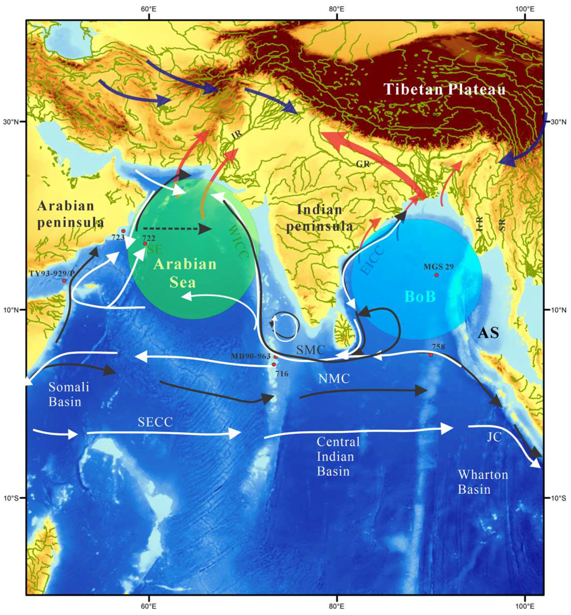
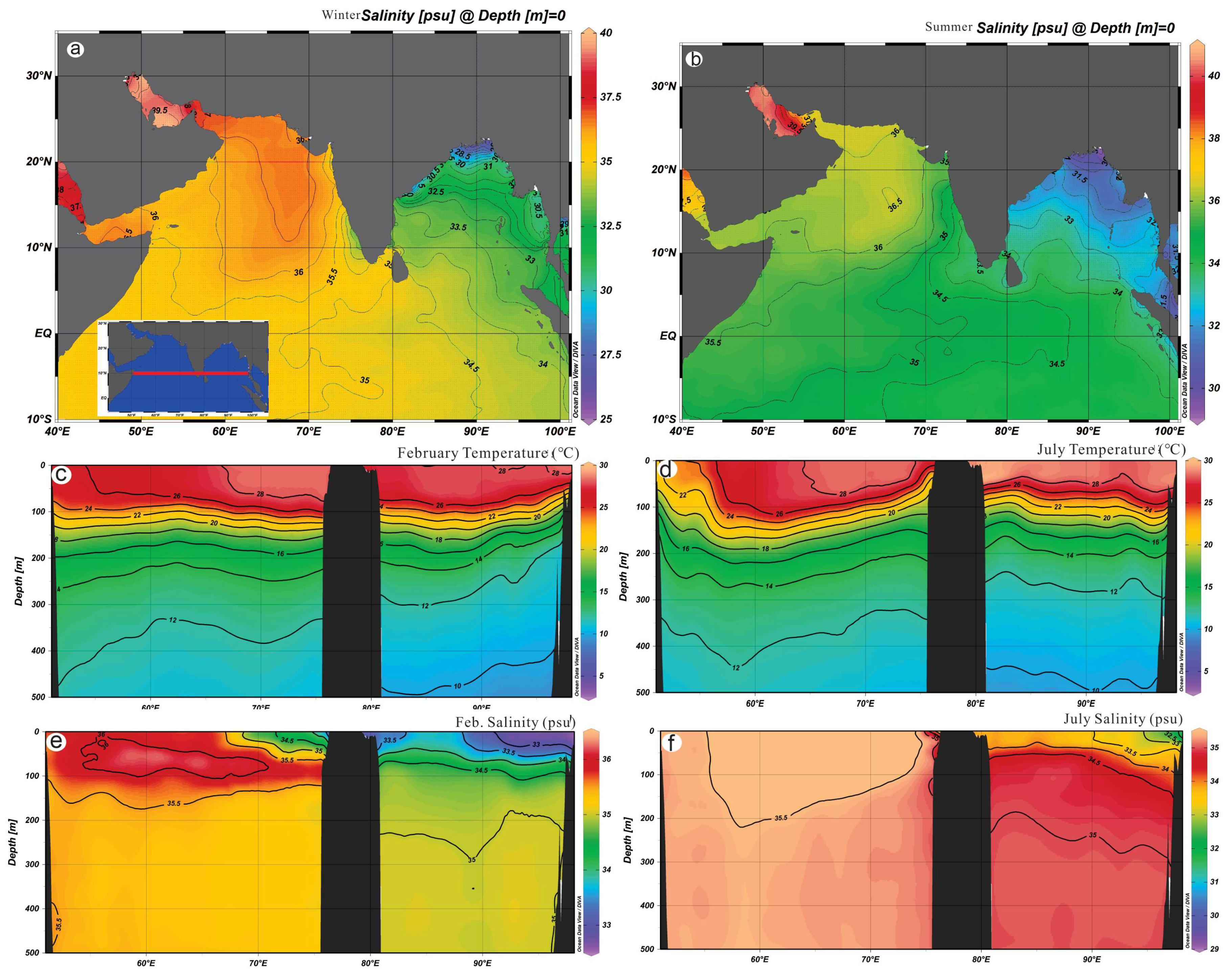
2. Modern Surface and Deep Circulation of the Indian Ocean

The GBM traverses the Indo-Gangetic plain and much of Bangladesh, draining freshwater from monsoonal rainfall [62] and ablating the Tibetan glaciers [63]. Moreover, the Brahmaputra River also receives freshwater from NE Indian highlands, Myanmar, and eastern Tibet. About 80% of the monsoonal rain falls on the GBM catchments (Figure 1), draining most of the Indo-Gangetic/Meghna plains and NW Myanmar [64,65]. As a result, ~1330 km3/yr of freshwater [66] discharges into the BoB [19] during the summer, directly determining the sea surface hydrography. In contrast to eastern and northern India, the Indus River mostly drains the NW plain of the Indian subcontinent and discharges into the eastern Arabian Sea [67].
The northern Indian Ocean surface currents reverse their direction synchronously with the SWM and NEM [17,68]. During the SWM, the East Indian Coastal Current (EICC) flows northward along the eastern Indian continental margin (Figure 1) in the BoB. Part of the EICC may also enter the Andaman Sea through its northern channel [69]. Moreover, the West Indian Coastal Current (WICC) follows the West Indian coast in the Arabian Sea and flows equatorward [68,70]. However, both the EICC and WICC reverse during the NEM. In winter, the westward-flowing North Equatorial Current (NEC) also brings surface waters through the Strait of Malacca, reaching 7.5° N in the BoB. The other notable surface circulations that change direction are the SWM and NEM currents (i.e., SMC and NMC), which link the western Java coastal waters by the Java Current to the Arabian Sea [68]. The westward-flowing South Equatorial Current (SEC) between 5° S and 15° S brings western Pacific waters through the Indonesian throughflow, occupying depths between 0.50 and 1.20 km [71,72,73]. At around 5° N of the Somali margin, these waters turn eastward and thus feed the thermocline.
Abram et al. [74] reviewed the Indian Ocean Dipole (IOD) and the ambiguous claims of its impact on the past Indian monsoons [75]. This brief description gives an important context for the IOD but does not claim to be an in-depth review of modern-day tropical Indian Ocean climate dynamics. The eastern equatorial Indian Ocean acts as a gateway through various straits between the western Pacific and Indian Ocean, which might modulate the impact of interannual-, annual-, decadal-, or longer-scale ocean-atmospheric events, namely, the El-Niño Southern Oscillation (ENSO), La-Niña, or IOD on the Indian monsoons. The IOD is most commonly defined based on the Dipole Mode Index (DMI) associated with the interannual SST oscillations between the eastern and western Indian Ocean in which the positive DMI phase is characterized by the high SST anomaly in the western Indian Ocean and cold SST anomaly in the east due to enhanced upwelling off the Java-Sumatra coast [76,77]. Thus, the positive and negative DMI impacted the zonal gradients and atmospheric convection over the tropical Indian Ocean and surrounding landmasses [76,78]. However, the extent to which the DMI exerts influence on the SWM is inadequately understood, most likely due to the geographical positions of the SST anomalies between the equatorial western Indian Ocean (10° S–10° N; 50° E–70° E) and the southeastern Indian Ocean (10° S–equator; 90° E–110° E) [76]. It is plausible that the DMI impacts the upwelling regions of the western Arabian Sea and, thus, affects the SWM; however, such an oceanographic link between the two regions remains to be established.
The mean February and July SSTs vary from 15 to 32.5 °C and 21 to 34 °C, respectively, whereas the salinities range from 28–41 and 27–40 psu (practical salinity unit) in the Arabian Sea and BoB (Figure 2). The mean sea surface salinities in the northern BoB and the Andaman Sea are the lowest (~24 psu) in August and the highest (34 psu) in May and generate a strong NE–SW salinity gradient [79]. The mean seasonal SSTs in the northern BoB are the coldest (~26 °C) during the winter and warmest (~28–29 °C) during the summer. The mixed-layer depths vary from 30 to 50 m (Figure 2) in February and July in the central BoB, in which the deepening of the mixed layer was attributed to the runoff during the SWM [20]. It is surprising to identify low-salinity (35.5 psu) cells cropping out on the coast of Somalia and a small, even lower-salinity (34.5 psu) cell along the southern tip of India, whereas a low-salinity cell appears in the BoB (Figure 2e) during February. In contrast to February, the low-salinity cells disappeared in the Arabian Sea due to positive E-P, and a low-salinity cell appeared in the eastern BoB during July, most likely due to the GBM runoff.
Unlike the Atlantic Ocean, which ventilates in the north in the Norwegian–Greenland–Labrador seas through North Atlantic Deep Water (NADW) formation and upwells in the south near the Antarctic Polar Front, the deep Indian Ocean only ventilates from the south. In the southeast, deep waters comprised of equal amounts of lower-circumpolar Deep Water (LCPDW) and Antarctic Bottom Water (AABW) [80] enter the Southeast Indian Ocean through the Perth Basin, providing about one-quarter of the global AABW [81,82]. This AABW originates from the Ross Sea, travels along the Wilkes-Adélie Coast [83,84,85], and spills into the Central Indian Basin through numerous deep gaps of the 90° E ridge [80,86]. In the southwest, waters entering into the Crozet-Madagascar and Mozambique basins are comprised of LCPDW (>3.8 km) and are overlain by the upper CPDW between 2 and 3.8 km [84]. These waters flow as the western boundary current into the Somali and Arabian basins after passing through the Amirante Passage [80,87]. In the northern Indian Ocean, the nutrient content of the northward-flowing deep waters progressively ages owing to the lack of ventilation and is not modified by mixing with any other deep-water mass [84,87,88]. The only deep-water mass that exits from the Indian Ocean is the Indian Deep Water in the 2–3.5 km range [84,87,89]. The Indian Deep Water, a mixture of upwelled bottom water and UCPDW, flows as the southward boundary current in the western Indian Ocean and has high silica, low oxygen, and high salinity [90,91].
The cold and dense AABW floods the deepest part of the Antarctic Ocean and moves northward to fill the global ocean. The Atlantic and Indian Oceans’ Antarctic Intermediate Water (AAIW) originates primarily in the Southeast Pacific just off Chile as a portion of the new AAIW flows eastward through the Drake Passage, north of the Subantarctic Front [92,93,94]. While passing through this passage, some modifications to AAIW occur, and newly formed intermediate waters are added by injecting surface waters into the subtropical gyre at the Brazil–Falkland Current confluence [95]. The AAIW can be traced as far north as 20° S in the Indian Ocean due to its low salinity and high nutrient and oxygen content [94,96]. High salinity (40 psu) intermediate waters are formed in the northwestern Indian Ocean through the inflow of Persian Gulf and Red Sea saline waters. Circulation patterns strongly influence the foraminiferal preservation in the various sub-basins of the Indian Ocean [97,98,99].

3. Materials and Methods

This study uses the published planktonic foraminiferal census by Frerichs [57], Guptha et al. [58], Brown University [51], Mohtadi et al. [55], Cortese et al. [59], Munz et al. [53], Anbuselvan and Nathan [52], Munir et al. [54], Bhadra and Saraswat [61], and Salman and Saraswat [50]. These data are plotted in Figure 3 and are listed in Table S1. These data mostly comprise sediment core tops, plankton nets, and tows, as reported by researchers. We have cleaned the data by identifying and deleting repetitive points from the same core sites to avoid overrepresentation in the kriging when plotting individual foraminiferal distributions. Notably, some of these data were part of the CLIMAP project [33,34], which was subsequently used by many publications, including the MARGO [100] project and other successive publications, without filtering. Moreover, Munz et al. [53] added 274 new data points to the MARGO dataset, primarily from the western Indian and eastern African margins, resulting in improved foraminiferal spatial maps.
The calcium carbonate, i.e., wtCaCO3%, from the bulk sediments was collected from 1241 core tops, both from the continental margin and deep sea, where the former appears to be highly influenced by the terrestrial sediments but the latter records pelagic sediments. These data were recently compiled by Zhang et al. [99] and Saraswat et al. [101], and this study is listed in Table S2. Unfortunately, the first wtCaCO3% data covering the entire Indian Ocean, reported by Kolla et al. [97], are lost (pers. comm., Kolla, January 2025).
An effort was made to collate total organic carbon data from the same predefined geographic region, with limited success due to a lack of published data or data that were gathered but remain unpublished. As a result, a more accurate measure of productivity cannot be assessed. However, recently, Saraswat et al. [101] reported data from 66 sediment samples from the Bay of Bengal and Andaman Sea, which were used to assess the impact of terrestrial discharge on CaCO3 concentration, thereby informing the foraminiferal census. Furthermore, Zhang et al. [99] compiled 689 core tops (i.e., late Holocene), CaCO3%, which were used to calculate particulate organic carbon from the Indian Ocean. This study uses all the available data to assess the productivity related to planktonic foraminiferal abundance.
There has always been an interest in understanding the relationship between present-day oceanographic conditions and modern faunas and floras, with the aim of reconstructing climatic variations in the Quaternary period. To date, three different approaches have been used to quantify the relationship between faunal data and the physical properties of the environment. The first approach, known as the Imbrie–Kipp transfer function (IKTF) method [30], employs the standard statistical technique of Q-mode principal component analysis to decompose the variation in the faunal census into a small number of variables, which are then regressed against the known physical parameters. Hutson [102] developed the modern analog technique (MAT), which searches the database of modern faunas of samples with an assemblage that most resembles the fossil assemblage. Those two approaches were significantly improved in the modern analog with the similarity index (SIMMAX) method [103] and the revised analog method (RAM) [104]. However, one contemporary approach is the use of artificial intelligence and machine learning, specifically artificial neural networks (ANNs), which rely on the assumption that there is a relationship between the distribution of modern faunas and the physical properties of the environment. Artificial neural networks (ANNs) can overcome problems associated with fuzzy and nonlinear relationships between sets of input and output variables. Once trained, the neural network serves as a unique transfer function; yet, at the same time, this nonlinear and recurrent function is so complex that it can simulate a decision-making algorithm. The available core top foraminiferal census from the northern Indian Ocean was cured following three criteria: (i) the record does not contain at least 15 foraminiferal species; (ii) records show a high degree of dissolution (e.g., a high % G. menardii); and (iii) high terrigenous input and siliceous fossils. Following these criteria, one hundred and ninety-four (194) core top (Figure 3b) foraminiferal censuses were regressed against the WCTs (i.e., 10 m, 100 m, and 200 m) using the modern oceanographic data from the 2023 WOA [20].
We have used 80% of the foraminiferal census to train the ANN model, and the rest of the data (i.e., 20%) was used for testing and validation, as shown in Figure 4. The model outputs show an excellent coefficient of correlation (R) of 0.928 during the summer, indicating that it performs well on the training set, with a strong linear relationship between predicted and actual values. The R-values between the predicted and actual values are 0.759 and 0.754 for the validation and test sets, respectively, suggesting that the model performs reasonably and satisfactorily compared to the training set (Figure 4). However, the overall R-value is 0.8709 when all the model results are pooled, which is considered good. In contrast to summer, the R-value is lower, i.e., 0.857, for winter. The extent to which factors contribute to a lower R-value for winter compared to summer is unclear. One of the possibilities for a foraminiferal census is a summer bias, such as a high percentage of G. ruber, G. sacculifer, etc., which requires further study and, thus, cannot be resolved at present.
The depth habitat and ecological niche of planktonic foraminifers in the tropical Indian Ocean are well known and are listed in Table 1. However, a few species, such as G. bulloides, G. glutinata, G. siphonifera, etc., mostly found on the continental margin, are briefly described here. G. bulloides is mostly found in the upwelling regions of the western Arabian Sea [14] and eastern BoB [58] and is considered a mixed-layer species. N. dutertrei has a high tolerance for low-salinity regions, such as in the northern BoB [58]. Likewise, G. rubescens, G. siphonifera, and G. glutinata were also found in similar environmental conditions [45,58].
The utility of ANNs in reconstructing past environmental conditions, including SSTs, was demonstrated in the North Atlantic [112,113] and for the latest short Holocene record [98] in a western Arabian Sea core, but the ANN technique has not been applied to the northern Indian Ocean for longer duration climate records. Therefore, this study chooses a foraminiferal census from core MGS29-GC02 [45] due to its higher resolution but short duration and ODP Site 758 [46], which has coarser resolution but longer duration (i.e., 890 ka) planktonic foraminiferal census and other available sediment geochemical data to test our ANN analytics.

4. Results and Discussion

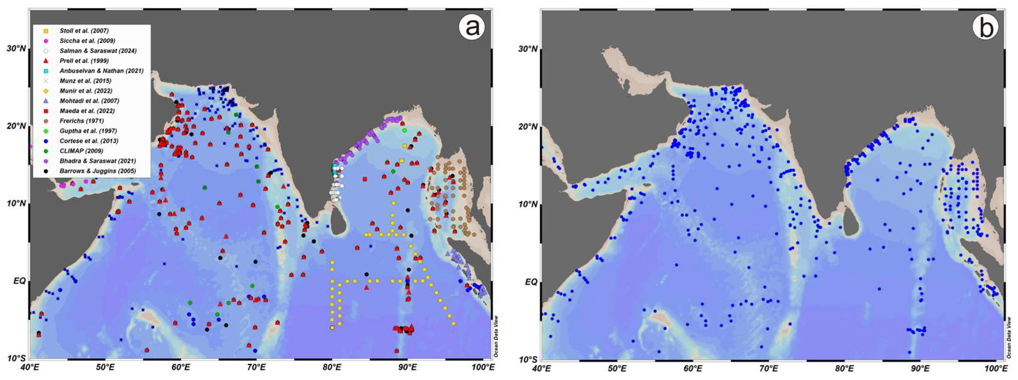
4.1. Relationships Between the Sediment Carbonate Concentration and Modern Foraminiferal Distribution

The sedimentary processes on the continental margin, pelagic sedimentation, and deep ocean circulation mostly influence the abundance of foraminiferal tests in sediments. This paradigm is well reflected by the distribution of various foraminifers and the lack of foraminiferal tests and <10% CaCO3 in deep basins, namely, the Wharton Basin, Central Indian Basin, Somali Basin, etc. (Figure 1, Figure 5 and Figure 6). The vast amount of terrigenous sediment discharge and associated freshwater dominate the continental shelf and upper slope of the BoB and the Andaman Sea during the SWM. As a result, the turbid water is likely to have an adverse effect on the ecology in the mixed layer and thermocline. This, in turn, impacts the foraminiferal concentration, as appears in Figure 5, either by limiting productivity or terrigenous dilution. For example, the foraminiferal spatial maps show scarce foraminiferal tests, whether on the BoB, Andaman Sea, or western Indian coast, irrespective of the species. Recently, Saraswat et al. [101] combined >700 surface samples from the BoB and Andaman Sea to demonstrate that the continental shelf and slope sediments contain <10% CaCO3, whereas the deepest part of the central northeast Indian Ocean, away from the mouth of GBM River systems, contains the highest %wtCaCO3 (Figure 5). These findings are consistent with the %wtCaCO3 concentration in the wider Indian Ocean, which has a limited supply of terrigenous sediments and siliceous fossils (e.g., diatoms). In contrast to the deep basins and continental margin, all the topographic highs, including most of the mid-Indian Ridge and the Ninety East Ridge, have high amounts of carbonates (Figure 5).
Three principal factors determine the foraminiferal concentration in the vast open Indian Ocean are the variations in (i) carbonate critical depth (CCrD; [114]), (ii) carbonate compensation depth (CCD; [115]), and (iii) the bottom water carbonate ion [CO32−] concentration [98]. Kolla et al. [97] adopted the CCrD (the depth below which less than 10% carbonate is present) for the Indian Ocean because of its relative ease of determination and comparison with published data from the Pacific and Atlantic oceans. The authors reported that the CCrD in the 10° N-0° region is 4500 m in the BoB, 4800 m in the Arabian Fan, and exceeds 5100 m in the Somali Basin. The CCrD is slightly deeper (i.e., 4800 m) in the 0–10° S region of the BoB compared to the 10° N–0°, whereas the CCrD is still over 5100 m in the Somali Basin. Cullen and Prell [38] assessed the CCD (where the carbonate input rate equals the carbonate dissolution rate) in the northern Indian Ocean, particularly noting that foraminiferal abundance decreases logarithmically in the equatorial region. In the eastern equatorial region, i.e., Wharton and Central Indian basins, whole tests are absent in sediments below 4600 m, while in the west (Somali Basin), whole tests are absent in the sediments below 5000 m (Figure 5).
Building on the works of Cullen and Prell [38], Peterson and Prell [98] reported multiple dissolution indices using a suite of sediment cores in the eastern equatorial Indian Ocean between 2° N and 15° S and 70° E and 104° E. The authors reported that the foraminiferal lysocline is located at approximately 3800 m in the eastern equatorial Indian Ocean, near the saturation horizon for calcite in the water column. Below the lysocline, the increase in foraminiferal fragmentation, decrease in absolute abundance, and progressive modification of planktonic foraminiferal assemblages with depth are accompanied by an increasing carbonate loss rate from the sediments. Moreover, Peterson and Prell [98] reported that up to 60% of planktonic foraminiferal tests in the >150 μm fractions were already broken at the depth of the lysocline, most likely due to the oxidation of organic matter incorporated into the sediments. Broecker and Takahashi [116] reported that the lysocline in the Atlantic and the Pacific oceans was associated with a critical carbonate ion concentration [CO32−], suggesting that dissolution is a thermodynamic process. Peterson and Prell [98] adopted the ∆CO32− (calcite), i.e., the difference between the in situ [CO32−] ion concentration of seawater and the saturation ion concentration [CO32−] for calcite at the in-situ temperature–pressure conditions. In this understanding, positive values of ∆CO32− represent supersaturation, and negative values indicate undersaturation of CaCO3 in seawater [117]. The ∆CO32− is principally governed by the circulation of IBW and AABW in the Indian Ocean, where the latter is undersaturated with CO32−. As a result, the deep Wharton and Central Indian basins do not show intact foraminifers even with the high productivity of calcite species in the equatorial Indian Ocean, as reflected in the CaCO3 in the 90° E ridge (Figure 5). It is one of the reasons dissolution-resistant species, e.g., G. menardii, G. dutertrei, etc. (Figure 6), show a higher concentration than the dissolution-prone species [38,99].

4.2. Modern Foraminiferal Distribution, Surface Currents, and Deep Circulation

The planktonic foraminiferal distribution reflects a combination of influence among the surface currents, deep circulation, and terrestrial supply along the continental margin in the Indian Ocean [97]. It is challenging to verify whether all core tops (Figure 6a) used in this study represent modern oceanographic conditions or even the late Holocene due to low sedimentation rates in parts of the tropical Indian Ocean due to great depths. However, this study followed the age assignment from the original publications despite acknowledging these discrepancies, which cannot be rectified at present. In addition, some core tops did not report full foraminiferal counts, resulting in a skewed concentration of certain foraminifera, which was considered when interpreting the impact of surface currents and deep circulation. For example, Cullen and Prell [38] grouped the 17 most abundant species in the northern Indian Ocean into three categories based on the foraminiferal lysocline (FL) using >250 geographically widespread surface sediment samples. The authors assigned (i) dissolution-resistant species, namely, G. menardii, G. tumida, G. dutertrei, and Pulleniatina obliquiloculata, which show a rapid and continuous increase in relative abundance at and below the FL; (ii) dissolution-susceptible species, namely, G. ruber, G. bulloides, and G. glutinata, exhibit a rapid and continuous decrease in relative abundance at and below the FL; and (iii) moderately susceptible species G. conglobatus, G. aequilateralis (now known as G. siphonifera), and G. conglomerata rapidly increase in abundance at the FL and systematically decrease with depth below FL. These foraminiferal groups provide a broader view of how to treat such large data to assess competing factors between preservation and dissolution. Munz et al. [53] excluded data from the BoB and the Red Sea due to “unique environmental forcing”; however, the authors used a variety of additional criteria to filter the data, such as high numbers of Sphaeroidinella dehiscens as an indicator of dissolution, grouping Globigerinella siphonifera and Globigerinella calida and Globorotalia menardii and Globorotalia tumida due to their morphological similarity [118], etc. In any event, this study has selected five dominant foraminifers, namely, G. ruber, G. sacculifer, G. bulloides, P. obliquiloculata, and Neogloboquadrina dutertrei that comprise nearly >80% of the total foraminiferal concentration of the dataset. In addition, we have chosen these five species due to their utility in reconstructing past upwelling, SST, and SSS ([18,39,55,119,120,121] and references thereafter). The spatial distribution of five species is illustrated in Figure 6, following Cullen and Prell [38], and their respective water mass indicator is listed in Table 1.
The distribution of % G. bulloides (Figure 6b) mostly follows the distribution patterns of Cullen and Prell [38], i.e., high % G. bulloides on the Oman and SW Indian margin, the BoB, and the Andaman Sea. However, three new high % G. bulloides regions emerged compared to the contour of Cullen and Prell [38] on the Somali margin, eastern equatorial Africa around 5° S, and Java coast, which could be attributed to the contribution by Mohtadi et al. [55], Munz et al. [53], and Munir et al. [54]. The high G. bulloides concentration in these tropical regions is mostly due to upwelling related to Ekman pumping and wind stress [14,122]. Moreover, the new G. bulloides spatial distribution on the western BoB margin is due solely to the contribution by Bhadra and Saraswat [61] and Salman and Saraswat [50]. One of the interesting points to note is the emergence of a high % G. bulloides east off Sri Lanka, which is most likely an artifact of the kriging method, as there are only two core tops on the Malabar coast (i.e., western Sri Lankan margin). Two white semi-circles centered at 80° E and 95° E suggest the absence of G. bulloides (Figure 6b), reflecting the lack of core tops (Figure 6a).
Both G. ruber (white variety) and G. sacculifer (Figure 6c,d) have identical abundances with <5% concentration on the Oman and Somali margins and Somali and Central Indian basins. However, G. ruber (w) is high in the BoB and western Indian continental margins, Andaman Sea, Java coast, and 90° E ridge (Figure 6c). Moreover, the new data show a high concentration of G. ruber (w) on the eastern African margin around 5° S and the Java coast, compared to the contour of Cullen and Prell [38]. The concentration of G. ruber in the equatorial region is patchy, most likely due to the impact of differential dissolution [37,98]. The contour of G. sacculifer (Figure 6d) on the wider Oman and Somali margins is identical to the distribution of Cullen and Prell [38], with < 5% that extends to the Pakistan margin. Three new high % G. sacculifer regions emerged in the new map on the Java coast, west of 90° E, around 8° S, and 5° S on the eastern African coast. The G. sacculifer distribution generally varies between 10 and 15% in most of the Central Indian Basin and the Bay of Bengal. The near absence of G. sacculifer in the Somali Basin and west of the Central Indian Basin is most likely due to the great depths that suffered significant dissolution [97,99].
The near identical distribution of N. dutertrei and P. obliquiloculata (Figure 6e,f) between 60° E and 70° E in the deep Somali Basin and the equatorial region reflects the preservation of relatively dissolution-resistant species at the expense of the dissolution-prone species [38,97]. Moreover, these two species are ubiquitous in the northern Indian Ocean with <10% concentration; however, these species are rare, especially P. obliquiloculata, with <2.5% on the continental margin of the BoB, Andaman Sea, western Indian coast, Persian Gulf, and Oman margin (Figure 6f). It is known that N. dutertrei lives in active current systems, along continental margins [38], as evident from its presence on the Somali upwelling site and the EICC (Figure 6e).
Globigerinita glutinata and Globorotalia menardii are cosmopolitan species in the northern Indian Ocean, although their distributions are patchy (not illustrated). The distribution of G. glutinata is identical to G. ruber (w), with >30% concentration on the Oman margin, the Gulf of Aden, and the Persian Gulf. However, it decreases to less than 20% on the western Indian coast and the west of the Andaman Sea. G. menardii is <10% in the Arabian Sea but >20% in the southern BoB [38].

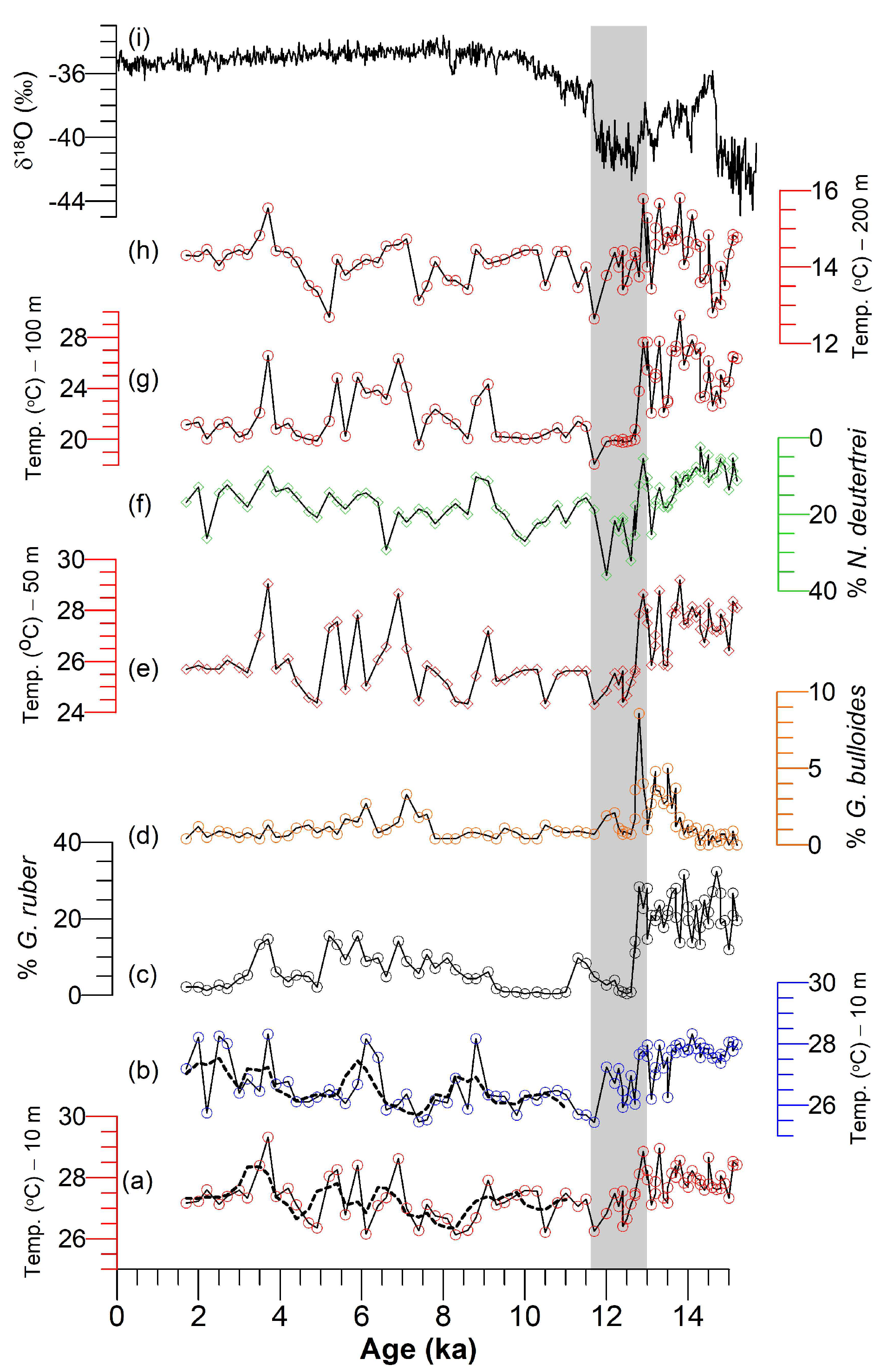
4.3. WCTs at the Northern and Southern Bay of Bengal Core MGS29-GC02 and Site 758

4.3.1. Northern Bay of Bengal WCTs from Core MGS29-GC02 During the Last 15 ka

We first applied our ANN code to a recently published northeastern BoB foraminiferal assemblage records from core MGS29-GC02 [45]. Gayathri et al. [45] reconstructed the water column characteristics by dividing the foraminiferal census data into two groups, i.e., salinity and productivity tracking species, during the past 15 ka. One of the interesting aspects of the data set is its high temporal resolution, ranging between 100 and 300 years, with only two 14C-AMS dates constraining the stratigraphy. Hence, the onset or demise of the abrupt climate events, namely, the warm Bolling–Allerød and cold Younger Dryas periods, may require further constraints when compared with the Greenland ice cores [123] or Indo-Asian speleothem records [124]. The average modern winter (Jan–March) and summer (July–Sept) temperatures at 10 m water depth of nearby core MGS29-GC02 are 27.35 °C and 28.77 °C [20], respectively. The age of the core top is 1.70 ka, in which the reconstructed WCTs at 10 m water depth in winter and summer are 27.19 °C and 27.17 °C, respectively (Figure 7a). Therefore, it is reasonable to assert that the ANN estimated WCTs are accurate within the limits of uncertainty, given the lack of a modern core top sample in core MGS29-GC02 and the uncertainty in foraminiferal census.
The warm WCTs at a 10 m water depth in summer and winter nicely match with high % G. ruber (Figure 7c) during the warm B/A period, consistent with the negligible concentration of upwelling species G. bulloides (Figure 7d). Lighter seawater oxygen isotopes (δ18Osw) in the Andaman Sea and the Bay of Bengal [18,125] further support a strengthened ISM during the B/A period. In contrast to the B/A, the high % G. bulloides, along with G. glutinata and the fertile species [45], suggest upwelling and nutrient-rich conditions during the YD, implying a weak SWM. Our reconstructed WCTs at a 10 m water depth in summer and winter (Figure 7a,b) and a 50 m water depth in summer (Figure 7e) are concordant with the weakened SWM.
The average winter and summer WCTs at a 10 m depth are 26.60 °C and 27.27 °C, respectively, consistent with a trace concentration of G. bulloides (Figure 7c). However, the % N. dutertrei inversely correlates with the WCT at a 50 m water depth during the Holocene compared to the deglacial period (15.20–12.90 ka), suggesting an enhanced ISM [45]. The enhanced ISM would precondition a freshwater environment, leading to a low-salinity environment in which high-tolerance species, such as N. dutertrei, G. rubescens, G. siphonifera, and G. glutinata, would thrive.

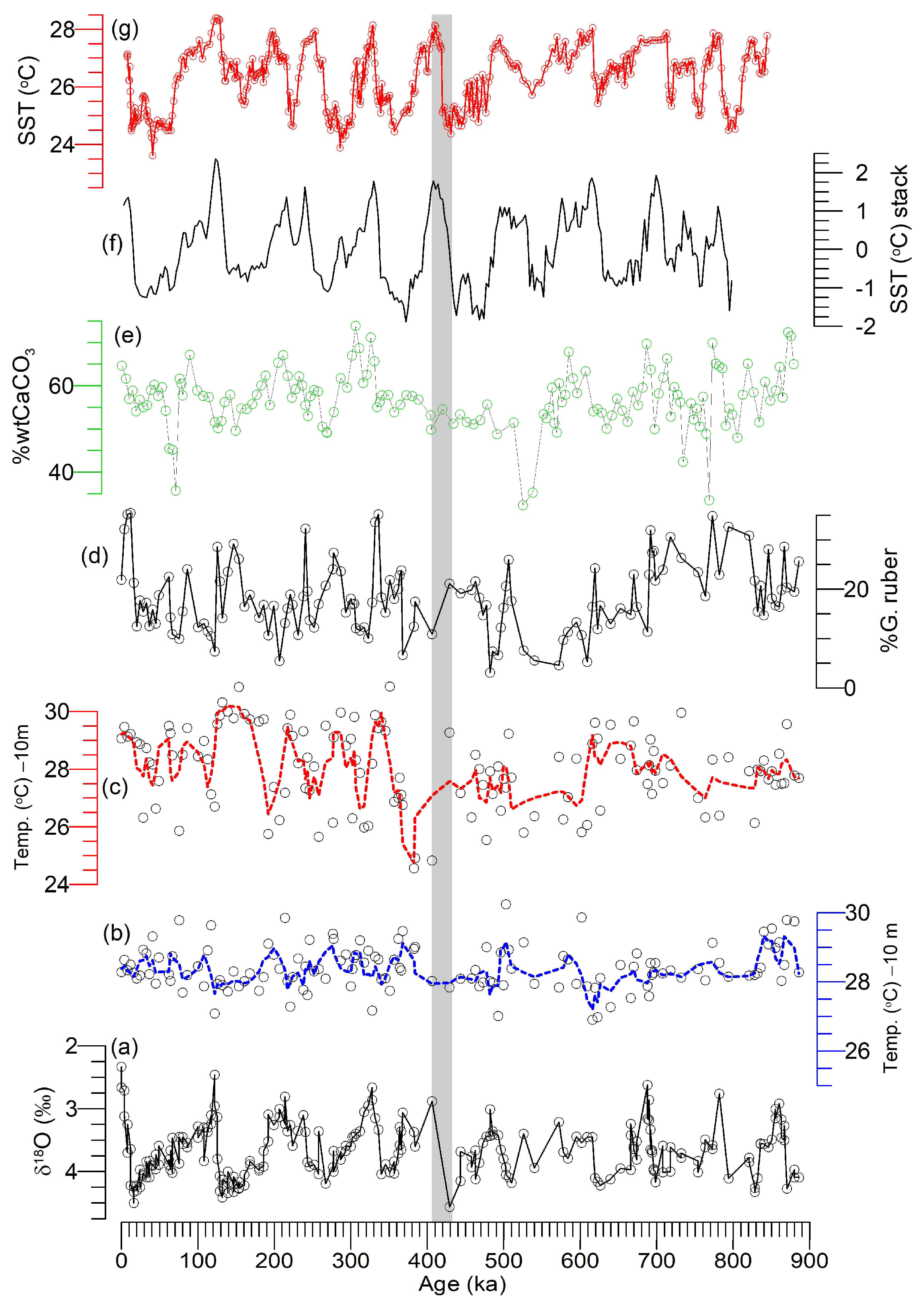
4.3.2. WCTs from the Southern Bay of Bengal ODP Site 758 During the Past 890 ka

The WCTs from Site 758 were plotted with the alkenones-derived SST from the Oman margin ODP Site 722 [126] in Figure 8 and the stacked global SST record [127]. The familiar glacial–interglacial cycles reported in the benthic δ18O record (Figure 8a) are absent in the WCTs at Site 758 (Figure 8b,c), although there appears to be a shift at 410 ka from an overall cooler climate before 410 ka to a warmer climate. Data from Site 758 are plotted following the age model of Chen and Farrell [46] to preserve data structure. Moreover, the temporal resolution is more than 9 kyrs; hence, the tentative boundary at 410 ka can be adjusted by updating the age model, which is not the focus of this study. In contrast to Site 758 WCTs, the alkenone-SSTs [115] from the western Arabian Sea ODP Site 722 (Figure 8g) reflect familiar glacial–interglacial cycles of the last 890 ka. It is known that there are differences in the paleo-proxy records due to inherent differences in depth habitats, ecology, and seasonality of the paleo-proxies, namely, alkenone-SST versus WCTs, as the former often represents the mean annual (for divergent views, see Stein et al. [128]) temperature [126] compared to the seasonal temperature by the latter (i.e., foraminifers). Moreover, Site 722 is influenced by upwelling during the summer, whereas Site 758 is mostly under the influence of seasonal reversal of the surface currents (Figure 1). However, it is clear that the alkenone-SSTs [126] reproduce the canonical glacial–interglacial cycles of the last 890 ka (Figure 8g) compared to the WCTs at Site 758 despite these differences. The benthic foraminiferal δ18O stratigraphy of Site 758 appears to have no irregularities as the δ18O curve reflects typical glacial–interglacial cycles [129], consistent with the global SST stack [127] or sea-level records [130]. Therefore, the one-step temperature shift at 410 ka (Figure 8) at Site 758 during the past 890 ka most likely suggests the impact of compounding factors on the estimation of WCTs. These factors are (i) an inaccurate ANN model (or code), (ii) foraminiferal ecology and habitats (Table 1), (iii) changes in the mixed-layer and thermocline temperatures, or (iv) complications with the foraminiferal census, which are briefly discussed below.
The algorithms used to formulate the ANN code are a simple backpropagation technique previously employed by earlier researchers, including Malmgren and Nordlund [131], Malmgren et al. [112], and Barrows and Juggins [43]. In this study, we followed the approach of Kucera et al. [132] and utilized a genetic algorithm to optimize the BP-ANN neural network. Additionally, we have successfully applied our ANN code to test the reproducibility of modern WCTs (see above; Figure 7) and key reference North Atlantic temperature records [133]. The successful reconstruction of the upper water temperature structure in the northern Bay of Bengal and North Atlantic (e.g., during the LGM) demonstrates the sensitivity of BP-ANN to reconstruct both cold and warm temperatures. Therefore, it is concluded that there are no significant errors in our ANN code when constructing modern and reconstructing past WCTs.
Numerous earlier studies [26,134,135] and a brief description in Section 3 and Section 4.2 provide information about the ecology and habitats of planktonic foraminifers worldwide, including the northern Indian Ocean. Hence, this study does not aim to provide an exhaustive description of foraminiferal ecology or habitats, nor is that its focus; however, most of the dominant species used in the ANN code for reconstructing the WCTs did not significantly alter their ecology or habitats during the Quaternary [34,132]. As such, this study hypothesizes that the foraminiferal depth habitats or ecology did not considerably impact the reconstructed WCTs shown in Figure 8.
A well-known modern climatological phenomenon, described in Section 2, i.e., the SWM dynamics, GBM outflow, and evaporation, results in changes in the northern BoB and Arabian Sea mixed layer and thermocline. It is reasonable to assume that near identical (i.e., late Holocene or the Present) climatic conditions prevailed during the past warm periods such as MIS 5e, 7e, 9e, and so on, thus recording similar mixed-layer and thermocline conditions. Moreover, climatic conditions during the cold periods, such as MIS 2, 4, 6, 10, and so on, would also be similar to the modern NEM conditions, i.e., less runoff and windy conditions, which may have weakened the stratification. Therefore, it is unreasonable to assume drastic changes in the mixed-layer and thermocline structure during the past 1 Ma, hence their negligible impact on the reconstructed WCTs.
Finally, the low-temperature interval between 415 ka and 370 ka (Figure 8) coincides with the onset of the mid-Brunhes evolution at 425 ka (considering the coarse temporal resolution and age model uncertainty), which could be attributed to the beginning of intense dissolution resulting in the low abundances of dissolution-prone species such as G. ruber and G. sacculifer. The low %wtCaCO3 (Figure 8e) [98] further supports this hypothesis. Site 758 is situated above the modern Indian Ocean CCD or CCrD [97,98]. However, the low %wtCaCO3 intervals associated with the cold periods must have a low bottom water [CO32−] concentration, which would have facilitated the dissolution. Low [CO32−]-bearing AABW must have flooded the Indian Ocean bottom water, including at Site 758, during those periods. In contrast to those periods, the NADW must have replaced the AABW during warm periods like the modern period, thus facilitating more foraminiferal test preservation. The coarse temporal resolution of the foraminiferal census prevented us from clearly assessing the lead and lag among the benthic foraminiferal δ18O, bulk sediments CaCO3, and WCTs at Site 758. Furthermore, one of the challenging tasks is the lack of a longer-duration, high-resolution foraminiferal census from the northern Indian Ocean to further test our ANN code. In this context, fresh sediments from the IODP Expeditions 354 (southern Bay of Bengal) and 355 (eastern Arabian Sea) could provide answers to many questions, thereby filling important gaps in our understanding of temperature evolution and monsoon dynamics [24].

4.4. Complexities in the Northern Indian Ocean’s Last Glacial Cycle Temperature Records

One of the complexities in reconstructing past sea surface temperatures (SSTs) or water column temperatures (WCTs) in the northern Indian Ocean is the divergence in temperature among paleo-proxies. We have plotted four SST records from the past 200 ka in the Indian Ocean to highlight the issues. For example, Herbert et al. [126] used alkenones (UK37) to reconstruct SSTs of the last 3.50 Ma from Site 722. In that record, the warmest SST during the MIS 5.5 and Holocene periods and cooler temperatures between 70 and 12 ka with minor warming centered at 30 ka (Figure 9d) were found during the last climatic cycle. In contrast to the open ocean Site 722, the Gulf of Aden core TY93-929/P (Figure 9e) suggests a gradual cooling that started from the optimum SST of about 28 °C at MIS 5.5 and continued up to 80 ka (Figure 9) using the same alkenone-derived SSTs. If the modern observational understanding of SWM is applied, it would suggest that MIS 5.5 would be associated with colder SSTs due to strong upwelling. Moreover, the coldest SSTs between 75 and 50 ka and 25 and 15 ka were interrupted by a warm interval between 40 and 22 ka (Figure 9). The interval between 25 and 15 can be loosely correlated to the deglaciation, including the LGM; however, the cooling between 75 and 50 ka is unprecedented in the northern tropics, as it coincides with colder MIS 4 and the warmer part of MIS 3.3.
The coldest SSTs during MIS 6 were generally 1–2 °C warmer than the coldest SSTs of the last glacial cycle. A potentially problematic limitation of UK37 is that lateral transport disproportionately impacts alkenone records. From the high-resolution Bermuda Rise drift site, Ohkouchi et al. [136] showed that radiocarbon dates in the alkenones are 7 kyr older than in the coexisting age of planktonic foraminifera. The authors reasoned that this temporal offset was likely due to the lateral transport of alkenones on fine-grained particles from the Nova Scotian margin, which markedly influenced estimates of SSTs [137]. Because alkenone carriers are very light (coccolithophores), they can travel long distances and have been shown to better record transport than local SST in areas characterized by vigorous surface currents such as the Agulhas Current [138] in the southwestern Indian Ocean. Therefore, the UK37-SST will show more divergence from SSTs reconstructed from other methods, such as foraminiferal assemblage-based MAT, radiolarian-based transfer function, and the Mg/Ca ratio. The extent to which lateral advection modulated the alkenone-SST in core TY93-929/P (Figure 9e) and Site 722 is unknown.
Figure 9. SST records from the northern Indian Ocean, including the western Arabian Sea. (a) Benthic foraminiferal oxygen isotopes (δ18O) in Site 758 [46]. The mixed-layer (i.e., 10 m water depth) temperature during the winter (b) and summer (c) of Site 758 were compared with three alkenone-derived SSTs from (d) western Arabian Sea Site 722 [126] and (e) piston core TY93929/P [139] and (f) Maldives Platform core MD90-963 [139]. All the records are plotted according to their published age models. The vertical grey bar represents the time interval of the penultimate deglaciation, whereas the discontinuous black line covering from (d) to (f) highlights the discrepancies in the onset of the cooling among the three SST records.
Geosciences 15 00241 g009
One of the starkest examples of divergences in SSTs among the paleo-proxies is reported from core MD79-257 in the southwestern Indian Ocean [120]. Levi et al. [138] have compared MAT-SST with those of the UK37-SST [140] from the same core MD79-257 and showed that the deglacial warming started around 18 ka in MAT-SST, whereas in the UK37-SST record, it started around 15.5 ka, thus demonstrating an offset of ~2.5 kyr for the same time horizon. Moreover, the MAT-SST reached Holocene SST by 14 ka, whereas UK37-SST slowly increased until 7 ka. In contrast to the western Arabian Sea sites (i.e., ODP 722 and TY TY93-929/P), the Maldives Platform core MD90-963 (i.e., northern Indian Ocean) does not show any temperature changes between MIS 6 and 5 but shows gradual (but minor) SST rise from 158 ka to 70 ka with a warm SST [139,141]. This trend could be superposed by the seasonality (<2 °C) during the last glacial cycle. Moreover, the overall cooling between 70 ka and 18 ka is in stark contrast with the Oman margin [126,127,128,129,130,131,132,133,134,135,136,137,138,139,140,141,142] and Site 758 records [46]. It is puzzling to note similar SST features for sites directly dominated by the SWM (i.e., Site 722 and TY TY93-929/P) and for a site mainly influenced by the NEM (MD90-963). Rostek et al. [141] offered two hypotheses to address the divergent SSTs. (i) The global warming recorded for MIS 5.5 could have counteracted and overwhelmed the seasonal cooling tied to the upwelling by the SWM. It is conceivable that the global cooling during glacial stages counteracted the seasonal warming associated with the weakened SWM upwelling. (ii) Strengthening the NEM during the cold periods was sufficient to mix the surface water column and create a seasonal cooling that canceled the weakening of the SWM upwelling. These are well-reasoned hypotheses; however, it is a challenging task to test them due to the low sedimentation rates in sediment cores from the northern equatorial Indian Ocean. Furthermore, these hypotheses do not explain the unprecedented cooling during MIS 3 and 2 compared to MIS 5 and 1. Pahnke and Sachs [142] suggested an increase in thermal gradients between the high and low to mid-latitudes at times of high-latitude ice sheet growth, implying an impact of the Northern Hemisphere cooling. However, the extent to which thermal gradients apply to the equatorial northern Indian Ocean must be worked out by obtaining high-resolution climate records and modeling results.

5. Conclusions

This study analyzed available foraminiferal census and bulk sediment carbonate data from sediment core tops and plankton tows and nets, spanning 25° N to 10° S and 40° E to 110° E. Various authors and institutions published most of these data between 1971 and 2024. However, this synthesis also used a few unpublished core tops’ foraminiferal censuses and carbonate data. Moreover, this study developed an artificial neural network (ANN) model to reconstruct water column temperatures (WCTs) by regressing the foraminiferal census of the core tops against modern oceanographic data from the northern Indian Ocean. Subsequently, the ANN code was successfully applied to the northern and southern Bay of Bengal core MGS29-GC02 and ODP Site 758 foraminiferal assemblage count to reconstruct the WCTs during the past 890 ka. The main conclusions are listed below.
(i)
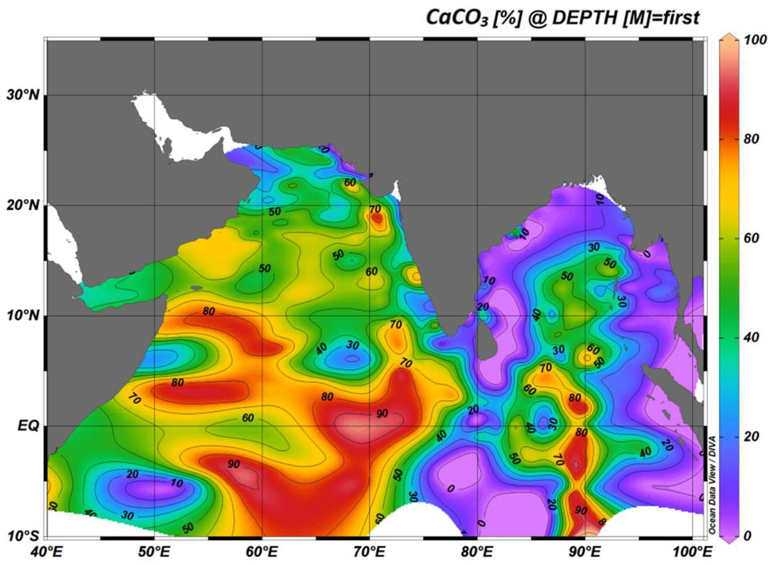
The improved spatial maps suggest that the low abundance of foraminiferal tests and % wtCaCO3 on the continental margin is most likely due to the large supply of terrigenous sediments borne by the numerous large rivers traversing the Indian subcontinent. However, the low % wtCaCO3 concentration and low abundance of foraminiferal tests in the deep basins such as the Somali Basin, Central Indian Basin, and Wharton Basin are due to the dissolution of carbonate as a result of intrusion by the low bottom water [CO32−]-bearing AABW.
(ii)
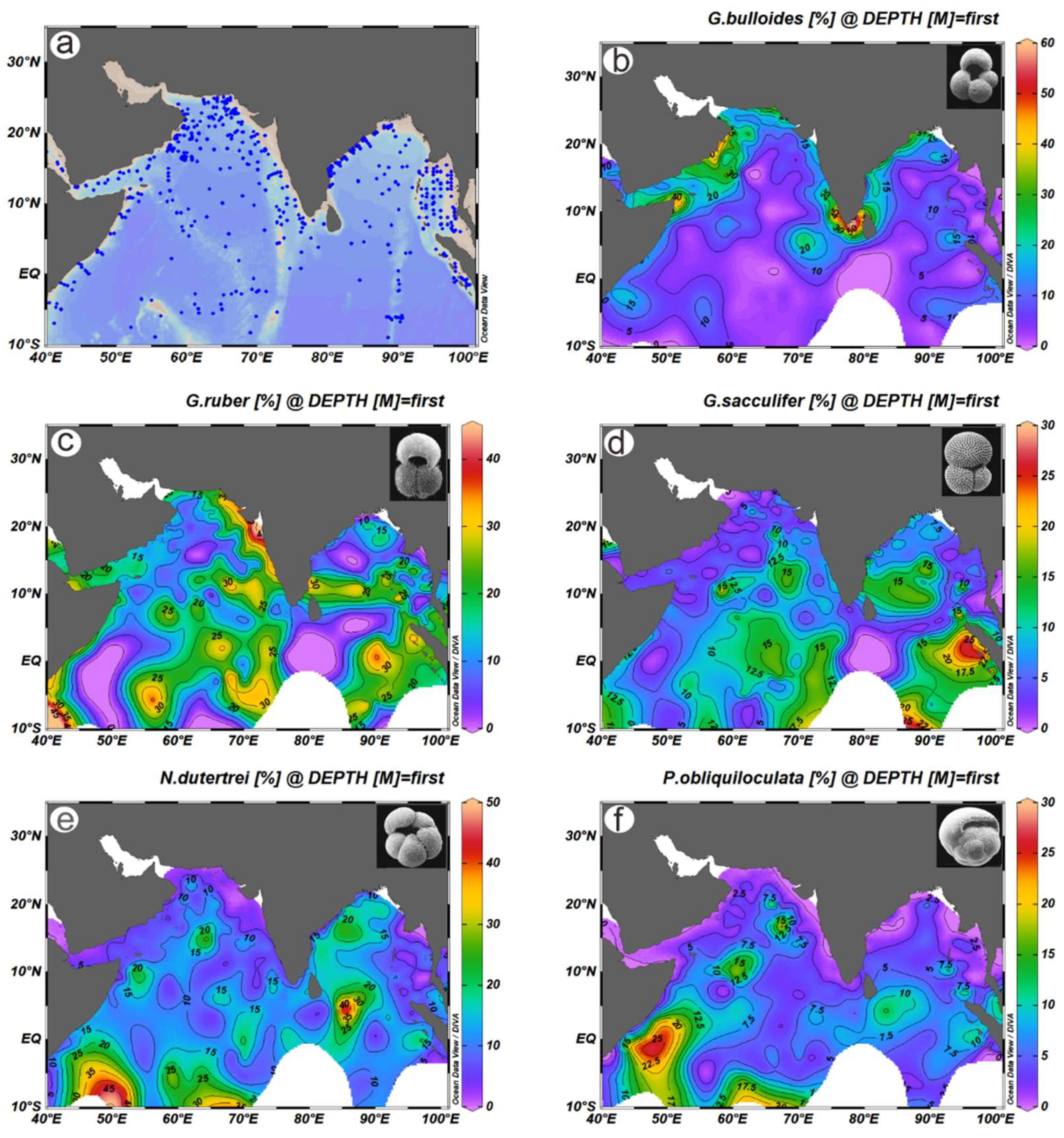
The most abundant Globigerinoides ruber (white), with a >30% concentration on the western Indian margin and southern equatorial Indian Ocean but >20% in the eastern Bay of Bengal, the Andaman Sea, and the Java coast, was found. The abundance of Globigerina bulloides is >30% in the upwelling region of the western Arabian Sea, but is also common (<10%) in the western BoB continental margin and the southern tip of India. G. sacculifer is ubiquitous in the northern Indian Ocean but is scarce in the western Arabian Sea. The abundance of Pulleniatina obliquiloculata is ~5%, with >10% scattered patches, but its abundance increases in the southwestern Indian Ocean. Neogloboquadrina dutertrei shows a near-identical distribution to P. obliquiloculata, except the former has a high concentration in the eastern Bay of Bengal. The dissolution-resistant characteristics of N. dutertrei and P. obliquiloculata tests facilitated their high preservation in the equatorial and southern Indian Ocean, even with the circulation of the Antarctic Bottom water. In contrast to the open Indian Ocean, the low foraminiferal concentration on the continental margin is most likely influenced by the terrestrial dilution.
(iii)
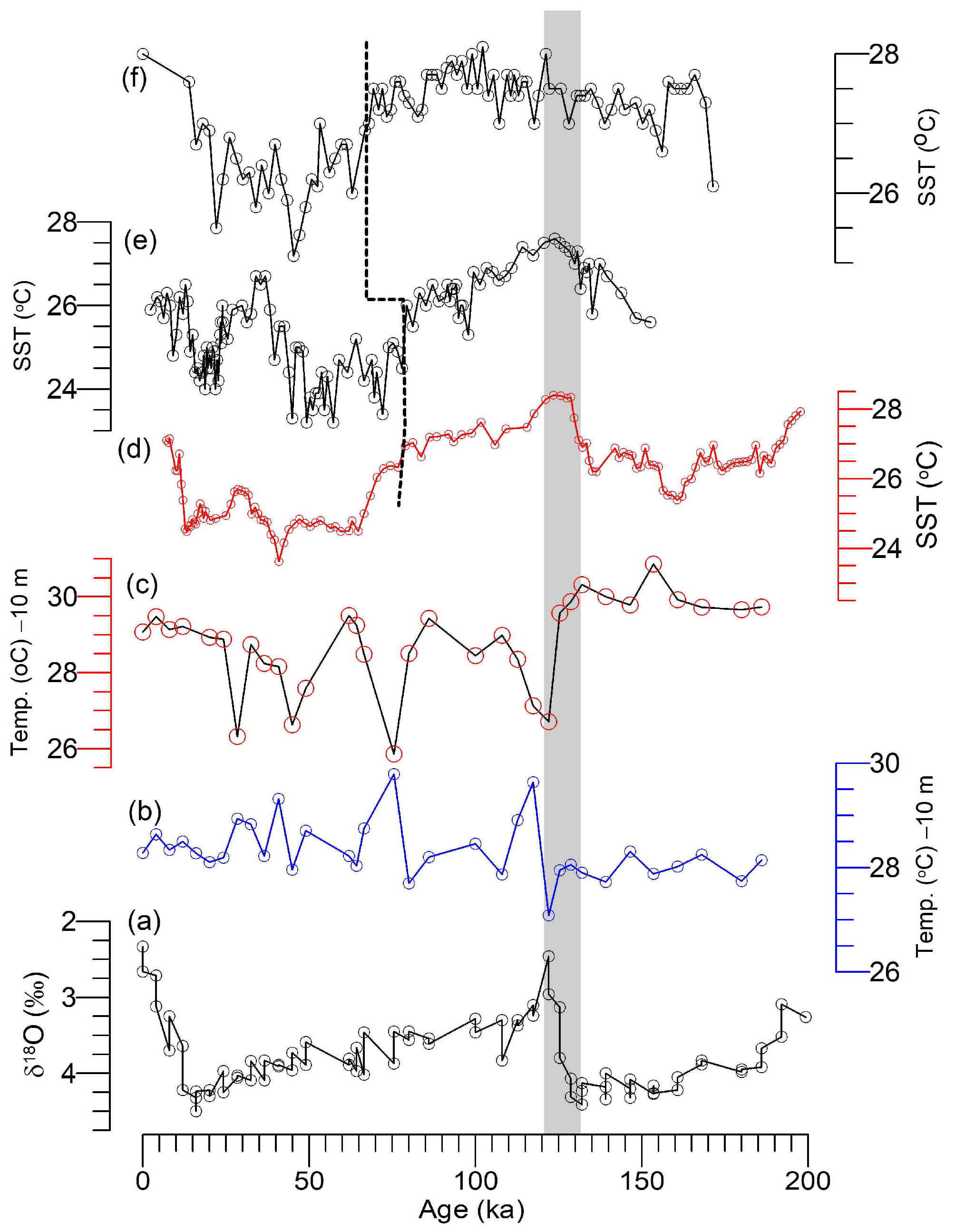
The reconstructed WCTs from core MGS29-GC02 suggest various influences from the freshwater during the Bolling–Allerǿd, Younger Dryas, and Holocene. Moreover, the WCTs from ODP Site 758 suggest a one-step change in the mixed-layer (i.e., 10 m water depth) temperature during the summer. However, no discernible change in temperature at 100 m and 200 m water depths was found. In contrast to ODP Site 758, the alkenone-derived sea-surface temperature at the western Arabian Sea ODP Site 722 shows canonical glacial–interglacial climate cycles of the last 1 Ma.
(iv)
There are divergences between the WCTs and alkenone-derived SSTs among the regional temperature composite, which could either be due to changes in depth habitats and seasonality in the paleo-proxies or be impacted by the upwelling of cold water.

Supplementary Materials

The following supporting information can be downloaded at https://www.mdpi.com/article/10.3390/geosciences15070241/s1; Figure S1: Water column temperature at 10 m, 100 m, and 200 m water depth of ODP Site 758; Tables S1 and S2: List of core locations used for Figure 3, Figure 5 and Figure 6.

Author Contributions

Conceptualization, H.R.; methodology, H.R. and Y.W.; validation, X.H. and C.K.S.; formal analysis, M.Z.; investigation, H.R. and M.Z.; resources, H.R.; data curation, X.H. and Y.W.; writing—original draft preparation, H.R. and X.H.; writing—review and editing, H.R., X.H., C.K.S. and M.Z.; visualization, X.H., Y.W. and C.K.S.; supervision, H.R.; project administration, H.R.; funding acquisition, H.R. All authors have read and agreed to the published version of the manuscript.

Funding

This research was funded by the National Natural Science Foundation of China, grant numbers 41976056 and 41776064.

Data Availability Statement

Data used in this article are archived at http://ed/nrcan.gc.ca/index_e.php (accessed on 18 June 2025) and are freely available.

Acknowledgments

Part of this study was conducted when the Atlantic Canada Opportunities Agency supported the senior author. M. Vermooten, Q.F. Sun, and A. Nur are acknowledged for their help in organizing published data. The Ocean Drilling Program (ODP) provided access to some parts of the data for this study.

Conflicts of Interest

The authors declare no conflicts of interest.

References

  1. Kutzbach, J.E.; Street-Perrott, F.A. Milankovitch forcing of fluctuations in the level of tropical lakes from 18 to 0 kyr BP. Nature 1985, 317, 130–134. [Google Scholar] [CrossRef]
  2. Webster, P.; Magana, V.O.; Palmer, T.; Shukla, J.; Thomas, R.; Yanai, M.; Yasunari, T. Monsoons: Processes, predictability, and the prospects for prediction. J. Geophy. Res. 1998, 1031, 14451–14510. [Google Scholar] [CrossRef]
  3. Mei, R.; Ashfaq, M.; Rastogi, D.; Leung, L.R.; Dominguez, F. Dominating Controls for Wetter South Asian Summer Monsoon in the Twenty-First Century. J. Climate 2015, 28, 3400–3419. [Google Scholar] [CrossRef]
  4. Hunt, K.M.R.; Fletcher, J.K. The relationship between Indian monsoon rainfall and low-pressure systems. Clim. Dyn. 2019, 53, 1859–1871. [Google Scholar] [CrossRef]
  5. Hurley, J.; Boos, W. A global climatology of monsoon low-pressure systems. Quarter. J. Roy. Meteoro. Soc. 2014, 141, 1049–1064. [Google Scholar] [CrossRef]
  6. Masson-Delmotte, V.P.; Zhai, A.; Pirani, S.L.; Connors, C.; Péan, S.; Berger, N.; Caud, Y.; Chen, L.; Goldfarb, M.I.; Gomis, M.; et al. (Eds.) Climate Change 2021: The Physical Science Basis; Contribution of Working Group I to the Sixth Assessment Report of the IPCC; Cambridge University Press: Cambridge, UK; New York, NY, USA, 2021. [Google Scholar]
  7. Gupta, A.K.; Anderson, D.M.; Overpeck, J.T. Abrupt changes in the Asian southwest monsoon during the Holocene and their links to the North Atlantic Ocean. Nature 2003, 421, 354–357. [Google Scholar] [CrossRef]
  8. Kathayat, G.; Sinha, A.; Breitenbach, S.; Tan, L.; Spötl, C.; Li, H.; Dong, X.; Zhang, H.; Ning, Y.; Allan, R.; et al. Protracted Indian monsoon droughts of the past millennium and their societal impacts. Proc. Nat. Acad. Sci. USA 2022, 119, e2207487119. [Google Scholar] [CrossRef]
  9. Sengupta, D.; Raj, B.; Shenoi, S. Surface freshwater from Bay of Bengal runoff and Indonesian Throughflow in the Tropical Indian Ocean. Geophy. Res. Lett. 2006, 33, L22609. [Google Scholar] [CrossRef]
  10. Geen, R.; Bordoni, S.; Battisti, D.S.; Hui, K. Monsoons, ITCZs, and the Concept of the Global Monsoon. Rev. Geophy. 2020, 58, e2020RG000700. [Google Scholar] [CrossRef]
  11. Bastia, F.; Equeenuddin, S.M. Spatio-temporal variation of water flow and sediment discharge in the Mahanadi River, India. Global Planet. Change 2016, 144, 51–66. [Google Scholar]
  12. Dey, S.; Dash, M.; Sasmal, K.; Jana, S.; Nadimpalli, J. Impact of river runoff on seasonal sea level, Kelvin waves, and East India Coastal Current in the Bay of Bengal: A numerical study using ROMS. Reg. Stud. Mar. Sci. 2020, 35, 101214. [Google Scholar] [CrossRef]
  13. Akhil, V.P.; Durand, F.; Lengaigne, M.; Vialard, J.; Keerthi, M.G.; Gopalakrishna, V.V.; Deltel, C.; Papa, F.; de Boyer Montégut, C. A modeling study of the processes of surface salinity seasonal cycle in the Bay of Bengal. J. Geophy. Res. Oceans 2014, 119, 3926–3947. [Google Scholar] [CrossRef]
  14. Curry, W.B.; Ostermann, D.R.; Guptha, M.V.S.; Ittekkot, V. Foraminiferal production and monsoonal upwelling in the Arabian Sea: Evidence from sediment traps. Geol. Soc. Lond. Sp. Pub. 1992, 64, 93–106. [Google Scholar] [CrossRef]
  15. Vishal, C.R.; Gauns, M.U.; Pratihary, A.K. Suboxic waters of the eastern Arabian Sea shelter secondary chlorophyll maximum dominated by heterotrophic dinoflagellate Pronoctiluca spp. (order Noctilucales). Eviron. Monitorin. Ass. 2025, 197. [Google Scholar] [CrossRef]
  16. Ganapati, P.M.; Murphy, V.S.R. Salinity and temperature variation of surface waters off the Visakhapatnam coast. Univ. Mem. Oceanogr. I 1954, 49, 125–142. [Google Scholar]
  17. Shankar, D.; Vinaychandran, P.N.; Unnikrishnan, A.S. The monsoon currents in the north Indian Ocean. Prog. Oceanogr. 2002, 52, 63–120. [Google Scholar] [CrossRef]
  18. Rashid, H.; Flower, B.P.; Poore, R.Z.; Quinn, T.M. A ~25 ka monsoon variability record from the Andaman Sea. Quat. Sci. Rev. 2007, 26, 2586–2597. [Google Scholar] [CrossRef]
  19. Murata, F.; Terao, T.; Hayashi, T.; Asada, H.; Matsumoto, J. Relationship between the atmospheric conditions at Dhaka, Bangladesh, and rainfall at Cherrapunjee, India. Nat. Hazards 2008, 44, 399–410. [Google Scholar] [CrossRef]
  20. Reagan, J.R.; Boyer, T.P.; García, H.E.; Locarnini, R.A.; Baranova, O.K.; Bouchard, C.; Cross, S.L.; Mishonov, A.V.; Paver, C.R.; Seidov, D.; et al. World Ocean Atlas 2023; Dataset: NCEI Accession 0270533; NOAA National Centers for Environmental Information: Asheville, NC, USA, 2024. [Google Scholar]
  21. Locarnini, R.A.; Mishonov, A.V.; Baranova, O.K.; Reagan, J.R.; Boyer, T.P.; Seidov, D.; Wang, Z.; Garcia, H.E.; Bouchard, C.; Cross, S.L.; et al. World Ocean Atlas 2023, Volume 1: Temperature. National Centers for Environmental Information (U.S.); NOAA Atlas NESDIS 89; NOAA National Centers for Environmental Information (NCEI): Silver Spring, MD, USA, 2024. [Google Scholar]
  22. Molnar, P.; England, P.; Martinod, J. Mantle Dynamics, Uplift of the Tibetan Plateau, and the Indian Monsoon. Rev. Geophy. 1993, 31, 357–396. [Google Scholar] [CrossRef]
  23. Raymo, M.E.; Ruddiman, W.F. Tectonic forcing of Late Cenozoic climate. Nature 1992, 359, 117–122. [Google Scholar] [CrossRef]
  24. Clift, P.D.; Betzler, C.; Clemens, S.C.; Christensen, B.; Eberli, G.P.; France-Lanord, C.; Gallagher, S.; Holbourn, A.; Kuhnt, W.; Murray, R.W.; et al. A synthesis of monsoon exploration in the Asian marginal seas. Sci. Drilling 2022, 31, 1–29. [Google Scholar] [CrossRef]
  25. Bé, A.W.H.; Hamlin, W.H. Ecology of Recent Planktonic Foraminifera: Part 3: Distribution in the North Atlantic during the Summer of 1962. Micropaleontology 1967, 13, 87–106. [Google Scholar] [CrossRef]
  26. Bé, A.W.H.; Tolderlund, D.S. Distribution and ecology of living planktic foraminifera in surface waters of the Atlantic and Indian oceans. In Micropaleontology of Oceans; Funnell, B.M., Riedel, W.R., Eds.; Cambridge University Press: New York, NY, USA, 1971; pp. 105–149. [Google Scholar]
  27. Rashid, H.; Lu, Q.-Q.; Zeng, M.; Wang, Y.; Zhang, Z.-W. Sea-Surface Characteristics of the Newfoundland Basin of the Northwest Atlantic Ocean during the Last 145,000 Years: A Study Based on the Sedimentological and Paleontological Proxies. Appl. Sci. 2021, 11, 3343. [Google Scholar] [CrossRef]
  28. Schafer, C.T.; Rashid, H. Can planktonic Foraminifera help to implement the New United Nations High Seas Treaty? Proc. Nova Scotian Inst. Sci. 2024, 53, 205–217. [Google Scholar]
  29. Zeng, M.; Rashid, H.; Zhou, Y.-X.; McManus, J.F.; Wang, Y. Dynamics of the subpolar gyre and transition zone of the North Atlantic during the last glacial cycle. Quarter. Sci. Rev. 2023, 314, 108215. [Google Scholar] [CrossRef]
  30. Imbrie, J.; Kipp, N.G. Chapter: A New Micropaleontological Method for Quantitative Paleoclimatology: Application to a Late Pleistocene Caribbean Core. In The Late Cenozoic Glacial Ages; Turekian, K., Ed.; Yale University Press: New Haven, CT, USA, 1971; pp. 71–181. [Google Scholar]
  31. Kipp, N.G. New transfer function for estimating past sea-surface conditions from seabed distribution of planktonic foraminifera in the North Atlantic. In Investigation of Late Quaternary Paleoceanography and Paleoclimatology; Cline, R.M., Hays, J.D., Eds.; Geological Society of America Memoir: Boulder, CO, USA, 1976; Volume 145, pp. 3–41. [Google Scholar]
  32. Hutson, W.H.; Prell, W.L. A Paleoecological Transfer Function, FI-2, for Indian Ocean Planktonic Foraminifera. J. Paleontol. 1980, 54, 381–398. [Google Scholar]
  33. CLIMAP Project Members. The surface of the ice-age Earth. Science 1976, 191, 1131–1137. [Google Scholar] [CrossRef]
  34. CLIMAP Project Members. Seasonal Reconstructions of the Earth’s Surface at the Last Glacial Maximum. Geol. Soc. Amer. Map Chart Ser. 1981, MC-36, 1–18. [Google Scholar]
  35. Prell and the Brown University group (1980, 1984). NOAA National Centers for Environmental Information. Available online: https://doi.org/10.25921/WMEJ-6P14 (accessed on 2 January 2025).
  36. Prell, W.L.; Hutson, W.H.; Williams, D.F.; Bé, A.W.H.; Geitzenauer, K.; Molfino, B. Surface circulation of the Indian Ocean during the last glacial maximum, approximately 18,000 yr B.P. Quat. Res. 1980, 14, 309–336. [Google Scholar] [CrossRef]
  37. Cullen, J.L. Microfossil evidence for changing salinity patterns in the Bay of Bengal over the last 20,000 years. Palaeogeo. Palaeoclim. Palaeoeco. 1981, 35, 315–356. [Google Scholar] [CrossRef]
  38. Cullen, J.L.; Prell, W.L. Planktonic foraminifera of the northern Indian Ocean: Distribution and preservation in surface sediments. Mar. Micropaleo. 1984, 9, 1–52. [Google Scholar] [CrossRef]
  39. Anderson, D.M.P.; Prell, W.L. A 300 kyr record of upwelling off Oman during the Late Quaternary: Evidence of the Asian Southwest Monsoon. Paleoceanography 1993, 8, 193–208. [Google Scholar] [CrossRef]
  40. Vénce-Peyré, M.-T.; Caulet, J.P.; Grazzini, C.V. Glacial/interglacial changes in the equatorial part of the Somali Basin (NW Indian Ocean) during the last 355 kyr. Paleoceanography 1997, 12, 640–648. [Google Scholar] [CrossRef]
  41. Vénce-Peyré, M.T.; Caulet, J.P.; Grazzini, C.V. Paleohydrographic Changes in the Somali Basin (5°N Upwelling and Equatorial Areas) During the Last 160 kyr, Based on Correspondence Analysis of Foraminiferal and Radiolarian Assemblages. Paleoceanography 1995, 10, 473–491. [Google Scholar] [CrossRef]
  42. De, S.; Sarker, S.; Gupta, A.K. Orbital and suborbital variability in the equatorial Indian Ocean as recorded in sediments of the Maldives Ridge (ODP Hole 716A) during the past 444 ka. In Monsoon Evolution and Tectonics–Climate Linkage in Asia; Clift, P.D., Tada, R., Zheng, H., Eds.; Geological Society of London: London, UK, 2010; Volume 342, pp. 17–27. [Google Scholar]
  43. Barrows, T.T.; Juggins, S. Sea-surface temperatures around the Australian margin and the Indian Ocean during the Last Glacial Maximum. Quat. Sci. Rev. 2005, 24, 1017–1047. [Google Scholar] [CrossRef]
  44. Bhadra, S.R.; Saraswat, R. A strong influence of the mid-Pleistocene transition on the monsoon and associated productivity in the Indian Ocean. Quat. Sci. Rev. 2022, 295, 107761. [Google Scholar] [CrossRef]
  45. Gayathri, N.M.; Sreevidya, E.; Sijinkumar, A.V.; Nath, B.N.; Sandeep, K.; Kurian, P.J.; Pankaj, K. Last 15 ka record of water column changes associated with Indian summer monsoon variability from the northeastern Bay of Bengal. Quat. Int. 2025, 723, 109713. [Google Scholar] [CrossRef]
  46. Chen, M.T.; Farrell, J.W. Planktonic Foraminifer Faunal Variations in the Northeastern Indian Ocean: A High-Resolution Record of the Past 800,000 Years from Site 758. In Proceedings of the Ocean Drilling Program, Scientific Results Vol. 121; Weissel, J., Peirce, J., Taylor, E., Alt, J., Eds.; Ocean Drilling Program: College Station, TX, USA, 1991; pp. 125–140. [Google Scholar]
  47. Yang, Y.-P.; Zhang, L.-L.; Yi, L.; Zhong, F.-C.; Lu, Z.-Y.; Wan, S.; Du, Y.-F.; Xiang, R. A contracting Intertropical Convergence Zone during the Early Heinrich Stadial 1. Nat Comm. 2023, 14, 4695. [Google Scholar] [CrossRef]
  48. Stoll, H.M.; Arevalos, A.; Burke, A.; Ziveri, P.; Mortyn, G.; Shimizu, N.; Unger, D. Seasonal cycles in biogenic production and export in Northern Bay of Bengal sediment traps. Deep Sea Res. Part (II) 2007, 54, 558–580. [Google Scholar] [CrossRef]
  49. Siccha, M.; Trommer, G.; Schulz, H.; Hemleben, C.; Kucera, M. Factors controlling the distribution of planktonic foraminifera in the Red Sea and implications for the development of transfer functions. Mar. Micropaleontol. 2009, 72, 146–156. [Google Scholar] [CrossRef]
  50. Salman, M.; Saraswat, R. Intrusion of Arabian Sea high salinity water and monsoon—Associated processes modulate planktic foraminiferal abundance and carbon burial in the southwestern Bay of Bengal. Environ. Sci. Pollut. Res. 2024, 31, 24961–24985. [Google Scholar] [CrossRef] [PubMed]
  51. Prell, W.; Martin, A.; Cullen, J.; Trend, M. NOAA. 1999. Available online: https://www.ncdc.noaa.gov/paleo-search/study/5908 (accessed on 2 January 2025).
  52. Anbuselvan, N.; Nathan, D.S. Distribution and environmental implications of planktonic foraminifera in the surface sediments of southwestern part of Bay of Bengal, India. J. Sed. Environ. 2021, 6, 213–235. [Google Scholar] [CrossRef]
  53. Munz, P.M.; Siccha, M.; Lückge, A.; Böll, A.; Kucera, M.; Schulz, H. Decadal-resolution record of winter monsoon intensity over the last two millennia from planktic foraminiferal assemblages in the northeastern Arabian Sea. Holocene 2015, 25, 1756–1771. [Google Scholar] [CrossRef]
  54. Munir, S.; Sun, J.; Morton, S.L.; Zhang, X.; Ding, C. Horizontal Distribution and Carbon Biomass of Planktonic Foraminifera in the Eastern Indian Ocean. Water 2022, 14, 2048. [Google Scholar] [CrossRef]
  55. Mohtadi, M.; Max, L.; Hebbeln, D.; Baumgart, A.; Krück, N.; Jennerjahn, T. Modern environmental conditions recorded in surface sediment samples off W and SW Indonesia: Planktonic foraminifera and biogenic compounds analyses. Mar. Micropaleontol. 2007, 65, 96–112. [Google Scholar] [CrossRef]
  56. Maeda, A.; Kuroyanagi, A.; Iguchi, A.; Gaye, B.; Rixen, T.; Nishi, H.; Kawahata, H. Seasonal variation of fluxes of planktic foraminiferal tests collected by a time-series sediment trap in the central Bay of Bengal during three different years. Deep Sea Res. Part (I) 2022, 183, 103718. [Google Scholar] [CrossRef]
  57. Frerichs, W.E. Planktonic foraminifera in the sediments of the Andaman Sea. J. Foram. Res. 1971, 1, 1–14. [Google Scholar] [CrossRef]
  58. Guptha, M.V.S.; Curry, W.B.; Ittekkot, V.; Muralinath, A.S. Seasonal variation in the flux of planktonic foraminifera: Sediments trap results from the Bay of Bengal, Northern Indian Ocean. J. Foram. Res. 1997, 27, 5–19. [Google Scholar] [CrossRef]
  59. Cortese, G.; Dunbar, G.B.; Carter, L.; Scott, G.; Bostock, H.; Bowen, M.; Crundwell, M.; Hayward, B.W.; Howard, W.; Martínez, J.I.; et al. Southwest Pacific Ocean response to a warmer world: Insights from Marine Isotope Stage 5e. Paleoceanography 2013, 28, 585–598. [Google Scholar] [CrossRef]
  60. CLIMAP Project Members (2009): Planktic Foraminifera Counts in Surface Sediment Samples [Dataset]. PANGAEA. Available online: https://doi.org/10.1594/PANGAEA.51927 (accessed on 18 June 2025).
  61. Bhadra, S.R.; Saraswat, R. The flux of planktic Foraminifera; sediment trap results from the Bay of Bengal, northern Indian Ocean. Deep-Sea Res. Part (II) 2021, 183, 104927. [Google Scholar] [CrossRef]
  62. Hasan, Z.; Akhter, S.; Kabir, A. Analysis of rainfall trends in southeast Bangladesh. J. Environ. 2014, 3, 51–56. [Google Scholar]
  63. Thompson, L.G.; Yao, T.; Davis, M.E.; Henderson, K.A.; Mosley-Thompson, E.; Lin, P.-N.; Beer, J.; Synal, H.-A.; Cole-Dai, J.; Bolzan, J.F. Tropical Climate Instability: The Last Glacial Cycle from a Qinghai-Tibetan Ice Core. Science 1997, 276, 1821–1825. [Google Scholar] [CrossRef]
  64. Papa, F.; Prigent, C.; Aires, F.; Jimenez, C.; Rossow, W.B.; Matthews, E. Interannual variability of surface water extent at global scale, 1993–2004. J. Geophys. Res. 2010, 115, D12111. [Google Scholar] [CrossRef]
  65. Robinson, R.A.J.; Brezina, C.A.; Parrish, R.R.; Horstwood, M.S.A.; Oo, N.W.; Bird, M.I.; Thein, M.; Walters, A.S.; Oliver, G.J.H.; Zaw, K. Large rivers and orogens: The evolution of the Yarlung Tsangpo–Irrawaddy system and the eastern Himalayan syntaxis. Gondwana Res. 2014, 26, 112–121. [Google Scholar] [CrossRef]
  66. Subramanian, V. Sediment load of Indian Rivers. Curr. Sci. 1993, 64, 928–930. [Google Scholar]
  67. Perry, G.D.; Duffy, P.B.; Miller, N.L. An extended data set of river discharges for validation of general circulation models. J. Geophy. Res. 1996, 101, 21339–21349. [Google Scholar] [CrossRef]
  68. Schott, F.A.; McCreary, J.P. The monsoon circulation of the Indian Ocean. Progr. Oceanog. 2001, 51, 1–123. [Google Scholar] [CrossRef]
  69. Chatterjee, A.; Shankar, D.; McCreary, J.P.; Vinayachandran, P.N.; Mukherjee, A. Dynamics of Andaman Sea circulation and its role in connecting the equatorial Indian Ocean to the Bay of Bengal. J. Geophys. Res. Oceans 2017, 122, 3200–3218. [Google Scholar] [CrossRef]
  70. Chaudhuri, A.; Shankar, D.; Aparna, S.G.; Amol, P.; Fernando, V.; Kankonkar, A.; Michael, G.S.; Satelkar, N.P.; Khalap, S.T. Observed variability of the West India Coastal Current on the continental slope from 2009–2018. J. Earth Syst. Sci. 2020, 129, 57. [Google Scholar] [CrossRef]
  71. Gordon, A. Indian-Atlantic transfer of thermocline water at the Agulhas Retroflection. Science 1985, 227, 1030–1033. [Google Scholar] [CrossRef] [PubMed]
  72. Wijffels, S.E.; Meyers, G. An Intersection of Oceanic Waveguides: Variability in the Indonesian Throughflow Region. J. Phys. Oceanog. 2003, 34, 1232–1253. [Google Scholar] [CrossRef]
  73. Talley, L.D. Freshwater transport estimates and the global overturning circulation: Shallow, deep and throughflow components. Progr. Oceanogr. 2008, 78, 257–303. [Google Scholar] [CrossRef]
  74. Abram, N.J.; Hargreaves, J.A.; Wright, N.M.; Thirumalai, K.; Ummenhofer, C.C.; England, M.H. Palaeoclimate perspectives on the Indian Ocean Dipole. Quat. Sci. Rev. 2020, 237, 106302. [Google Scholar] [CrossRef]
  75. Zhou, X.-Q.; Alphonse, S.D.; Shi, X.-X.; Bassinot, F.; Moreno, E.; Jin, X.-B.; Beaufort, L.; Liu, C.-L. Changes in Atmospheric Convection Over the Indo-Pacific Warm Pool and Coupled IOD and ENSO Patterns During the Last Glacial Maximum. Geophys. Res. Lett. 2025, 52, e2024GL112276. [Google Scholar] [CrossRef]
  76. Saji, N.H.; Goswami, B.N.; Vinayachandran, P.N.; Yamagata, T. A dipole mode in the tropical Indian Ocean. Nature 1999, 401, 360–363. [Google Scholar] [CrossRef]
  77. Saji, N.H.; Xie, S.-P.; Tam, C.-Y. Satellite observations of intense intraseasonal cooling events in the tropical south Indian Ocean. Geophys. Res. Lett. 2006, 33, L14704. [Google Scholar] [CrossRef]
  78. Cai, W.-J.; Wu, L.-X.; Lengaigne, M.; Li, T.; McGregor, S.; Kug, J.-S.; Yu, J.-Y.; Stuecker, M.F.; Santoso, S.; Li, X.-C.; et al. Pantropical climate interactions. Science 2019, 363, eaav4236. [Google Scholar] [CrossRef]
  79. Gordon, A.L.; Shroyer, E.L.; Mahadevan, A.; Sengupta, D.; Freilich, M. Bay of Bengal: 2013 northeast monsoon upper-ocean circulation. Oceanography 2016, 29, 82–91. [Google Scholar] [CrossRef]
  80. Srinivasan, A.; Garraffo, Z.; Iskandarani, M. Abyssal circulation in the Indian Ocean from a 1/12° resolution global hindcast. Deep Sea Res. Part (I) 2009, 56, 1907–1926. [Google Scholar] [CrossRef]
  81. Rintoul, S.R.; Bullister, J.L. A late winter hydrographic section from Tasmania to Antarctica. Deep Sea Res. Part (I) 1999, 46, 1417–1454. [Google Scholar] [CrossRef]
  82. Sloyan, B.M. Antarctic bottom and lower circumpolar deep water circulation in the eastern Indian Ocean. J. Geophy. Res. 2006, 111, C02006. [Google Scholar] [CrossRef]
  83. Warren, B.A. Transindian hydrographic section at Lat. 18°S: Property distributions and circulation in the South Indian Ocean. Deep-Sea Res. 1981, 28, 759–788. [Google Scholar] [CrossRef]
  84. Mantyla, A.; Reid, J. On the origins of deep and bottom waters of the Indian Ocean. J. Geophy. Res. 1995, 100, 2417–2439. [Google Scholar] [CrossRef]
  85. Fukamachi, Y.; Rintoul, S.R.; Church, J.A.; Aoki, S.; Sokolov, S.; Rosenberg, M.A.; Wakatsuchi, M. Strong export of Antarctic Bottom Water east of the Kerguelen plateau. Nat. Geosci. 2010, 3, 327–331. [Google Scholar] [CrossRef]
  86. Warren, B.A.; Johnson, G.C. The overflows across the Ninety-east Ridge. Deep-Sea Res. (II) 2002, 49, 1423–1439. [Google Scholar]
  87. Johnson, G.C.; Musgrave, D.L.; Warren, B.A.; Ffield, A.; Olson, D.B. Flow of Bottom and Deep Water in the Amirante Passage and Mascarene Basin. J. Geophy. Res. 1998, 103, 30973–30984. [Google Scholar] [CrossRef]
  88. Orsi, A.H.; Jacobs, S.S.; Gordon, A.L.; Visbeck, M. Cooling and ventilating the Abyssal Ocean. Geophy. Res. Lett. 2001, 28, 2923–2926. [Google Scholar] [CrossRef]
  89. Rashid, H.; Wang, Y.; Gourlan, A.T. Impact of climate on past Indian monsoon and circulation: A perspective based on radiogenic and trace metal geochemistry. Atmosphere 2021, 12, 330. [Google Scholar] [CrossRef]
  90. Reid, J.L. On the total geostrophic circulation of the Indian Ocean: Flow patterns, tracers, and transports. Prog. Oceanogr. 2003, 56, 137–186. [Google Scholar] [CrossRef]
  91. Srinivasan, A.; Top, Z.; Schlosser, P.; Hohmann, R.; Iskandarani, M.; Olson, D.B.; Lupton, J.E.; Jenkins, W.J. Mantle 3He distribution and deep circulation in the Indian Ocean. J. Geophy. Res. 2004, 109, C06012. [Google Scholar] [CrossRef]
  92. England, M.H.; Godfrey, J.S.; Hirst, A.C.; Tomczak, M. The mechanism for Antarctic Intermediate Water renewal in a world ocean model. J. Phy. Oceanogr. 1993, 23, 1553–1560. [Google Scholar] [CrossRef]
  93. Toggweiler, J.R.; Bjornsson, H. Drake Passage and palaeoclimate. J. Quarter. Sci. 2000, 15, 319–328. [Google Scholar] [CrossRef]
  94. Talley, L.D.; Pickard, G.L.; Emery, W.J.; Swift, J.H. Descriptive Physical Oceanography: An Introduction, 6th ed.; Elsevier: Amsterdam, The Netherlands, 2011; p. 555. [Google Scholar]
  95. Talley, L.D. Antarctic Intermediate Water in the South Atlantic. In The South Atlantic: Present and Past Circulation; Wefer, G., Berger, W.H., Siedler, G., Webb, D., Eds.; Springer: Berlin/Heidelberg, Germany, 1996; pp. 219–238. [Google Scholar]
  96. Kroopnick, P.M. The distribution of C of δCO2 in the world oceans. Deep-Sea Res. (A) 1985, 32, 57–84. [Google Scholar] [CrossRef]
  97. Kolla, V.; Bé, A.W.H.; Biscaye, P.E. Calcium carbonate distribution in the surface sediments of the Indian Ocean. J. Geophy. Res. 1976, 15, 2605–2616. [Google Scholar] [CrossRef]
  98. Peterson, L.C.; Prell, W.L. Carbonate dissolution in Recent sediments of the eastern equatorial Indian Ocean: Preservation patterns and carbonate loss above the lysocline. Mar. Geol. 1985, 64, 259–290. [Google Scholar] [CrossRef]
  99. Zhang, H.-D.; Luo, Y.-M.; Yu, J.-M.; Zhang, L.-L.; Xiang, R.; Yu, Z.-J.; Huang, H. Indian Ocean sedimentary calcium carbonate distribution and its implications for the glacial deep ocean circulation. Quat. Sci. Rev. 2022, 28, 107490. [Google Scholar] [CrossRef]
  100. Kucera, M.; Rosell-Melé, A.; Schneider, R.; Waelbroeck, C.; Weinelt, M. Multiproxy approach for the reconstruction of the glacial ocean surface (MARGO). Quat. Sci. Rev. 2005, 24, 813–819. [Google Scholar] [CrossRef]
  101. Saraswat, R.; Fathima, R.; Salman, M.; Suokhrie, T.; Saalim, S.M. Decoupling of carbon burial from productivity in the northeast Indian Ocean. Sci. Total Environ. 2024, 947, 174587. [Google Scholar] [CrossRef]
  102. Hutson, W.H. Transfer functions under no-analog conditions: Experiments with Indian Ocean planktonic foraminifera. Quat. Res. 1977, 8, 355–361. [Google Scholar] [CrossRef]
  103. Pflaumann, U.; Duprat, J.; Pujol, C.; Labeyrie, L. SIMMAX: A modern analog technique to deduce Atlantic Sea surface temperatures from planktonic foraminifera in deep-sea sediments. Paleoceanography 1996, 11, 15–36. [Google Scholar] [CrossRef]
  104. Waelbroeck, C.; Labeyrie, L.; Duplessy, J.C.; Joel, G.; Labracherie, M.; Leclaire, H.; Duprat, J. Improving paleo-SST estimates based on planktonic fossil faunas. Paleoceanography 1998, 13, 272–283. [Google Scholar] [CrossRef]
  105. Bé, A.W.H. Foraminifera families: Globigerinidae and Globorotaliidae. In Fiches D’identification du Zooplancton; Charlottenlund Slot; International Council for the Exploration of the Sea: Copenhagen, Denmark, 1967; Sheet 108; pp. 1–9. [Google Scholar]
  106. Ravelo, A.C.; Fairbanks, R.G. Reconstructing tropical Atlantic hydrography using planktonic foraminifera and an ocean model. Paleoceanography 1990, 5, 409–431. [Google Scholar] [CrossRef]
  107. Thiede, J.; Junger, B. Faunal and floral indicators of coastal upwelling (NW African and Peruvian Continental Margins). In Upwelling Systems: Evolution Since the Early Miocene; Summerhayes, C.P., Prell, W.L., Emeis, K.C., Eds.; Geological Society of London: London, UK, 1992; Volume 64, pp. 47–76. [Google Scholar] [CrossRef]
  108. Kroon, D. Distribution of extant planktic foraminiferal assemblages in the Red Sea and northern Indian Ocean surface waters. In Planktonic Foraminifera as Tracers of Ocean Climate History; Brummer, G.J.A., Kroon, D., Eds.; Free University Press: Amsterdam, The Netherlands, 1988; pp. 229–267. [Google Scholar]
  109. Sautter, L.R.; Thunell, R.C. Planktonic foraminiferal response to upwelling and seasonal hydrographic conditions: Sediment trap results from San Pedro Basin, Southern California Bight. J. Foraminifer. Res. 1991, 21, 347–363. [Google Scholar] [CrossRef]
  110. Fairbanks, R.G.; Wiebe, P.H. Foraminifera and chlorophyll maximum: Vertical distribution, seasonal succession, and paleoceanographic significance. Science 1980, 209, 1524–1526. [Google Scholar] [CrossRef]
  111. Fairbanks, R.G.; Sverdlove, M.; Free, R.; Wiebe, P.H.; Bé, A.W.H. Vertical distribution and isotopic fractionation of living planktonic foraminifera from the Panama basin. Nature 1982, 298, 841–844. [Google Scholar] [CrossRef]
  112. Malmgren, B.A.; Kučera, M.; Nyberg, J.; Waelbroeck, C. Comparison of statistical and artificial neural network techniques for estimating past sea surface temperatures from planktonic foraminifer census data. Paleoceanography 2001, 16, 520–530. [Google Scholar] [CrossRef]
  113. Singh, H.; Singh, A.; Tripathi, R.; Singh, P.; Verma, K.; Voelker, A.; Hodell, D. Centennial-millennial scale ocean-climate variability in the northeastern Atlantic across the last three terminations. Global Planet. Change 2023, 223, 104100. [Google Scholar] [CrossRef]
  114. Lisitzin, A.P.; Petelin, V.P. Features of distribution and modification of CaCO3 in bottom sediments of the Pacific Ocean. Lihol. Miner. Resour. 1976, 5, 565–578. [Google Scholar]
  115. Bramlette, M.N. Pelagic sediments. In Oceanography; Sears, M., Ed.; American Association for the Advancement of Science: Washington, DC, USA, 1961; pp. 345–366. [Google Scholar]
  116. Broecker, W.S.; Takahashi, T. Neutralization of fossil fuel CO2 by marine calcium carbonate. In The Fate of Fossil CO2 in the Oceans; Springer: New York, NY, USA, 1977. [Google Scholar]
  117. Broecker, W.S.; Peng, T.-H. The role of CaCO3 compensation in the glacial to interglacial atmospheric CO2 change. Glob. Biogeoch. Cycle 1987, 1, 15–29. [Google Scholar] [CrossRef]
  118. Weiner, A.K.M.; Weinkauf, M.F.G.; Kurasawa, A.; Darling, K.F.; Kucera, M. Genetic and morphometric evidence for parallel evolution of the Globigerinella calida morphotype. Mar. Micropaleo. 2015, 114, 19–35. [Google Scholar] [CrossRef]
  119. Anand, P.; Kroon, D.; Singh, A.D.; Ganeshram, R.S.; Ganssen, G.; Elderfield, H. Coupled sea surface temperature–seawater δ18O reconstructions in the Arabian Sea at the millennial scale for the last 35 ka. Paleoceanography 2008, 23, PA4207. [Google Scholar] [CrossRef]
  120. Rashid, H.; Otieno, F.O.; Konfirst, K.M. Comments on “Does the Agulhas Current amplify global temperatures during super-interglacials?”. J. Quat. Sci. 2011, 26, 866–869. [Google Scholar] [CrossRef]
  121. Saraswat, R.; Lea, D.; Nigam, R.; Mackensen, A.; Naik, D. Deglaciation in the tropical Indian Ocean driven by the interplay between the regional monsoon and global teleconnections. Earth Planet. Sci. Lett. 2013, 375, 166–175. [Google Scholar] [CrossRef]
  122. Mathew, S.; Mathur, M. Anomalous sea surface temperature over the Southeastern Arabian Sea during contrasting Indian Ocean Dipole years. Clim. Dynam. 2025, 75, 1–18. [Google Scholar] [CrossRef]
  123. Rasmussen, S.O.; Bigler, M.; Blockley, S.P.; Blunier, T.; Buchardt, S.L.; Clausen, H.B.; Cvijanovic, I.; Jensen, D.D.; Johnsen, S.J.; Fischer, H.; et al. A stratigraphic framework for abrupt climatic changes during the Last Glacial period based on three synchronized Greenland ice-core records: Refining and extending the INTIMATE event stratigraphy. Quat. Sci. Rev. 2014, 106, 1428. [Google Scholar] [CrossRef]
  124. Dutt, S.; Gupta, A.K.; Clemens, S.C.; Cheng, H.; Singh, R.K.; Kathayat, G.; Edwards, R.L. Abrupt changes in Indian summer monsoon strength during 33,800 to 5500 years B.P. Geophys. Res. Lett. 2015, 42, 5526–5532. [Google Scholar] [CrossRef]
  125. Liu, S.-F.; Ye, W.-X.; Chen, M.-T.; Pan, H.-J.; Cao, P.; Zhang, H.; Khokiattiwong, S.; Kornkanitnan, N.; Shi, X.-F. Millennial-scale variability of Indian summer monsoon during the last 42 kyr: Evidence based on foraminiferal Mg/Ca and oxygen isotope records from the central Bay of Bengal. Palaeogeogr. Palaeoclimatol. Palaeoecol. 2021, 562, 110112. [Google Scholar] [CrossRef]
  126. Herbert, T.D.; Peterson, L.C.; Lawrence, K.T.; Liu, Z.-H. Tropical Ocean Temperatures Over the Past 3.5 Million Years. Science 2010, 328, 1530–1534. [Google Scholar] [CrossRef]
  127. Shakun, J.D.; Lea, D.W.; Lisiecki, L.E.; Raymo, M.E. An 800-kyr record of global surface ocean and implications for ice volume-temperature coupling. Earth Planet. Sci. Lett. 2015, 428, 58–68. [Google Scholar]
  128. Stein, R.; Hefter, J.; Grützner, J.; Voelker, A.H.L.; Naafs, B.D.A. Variability of surface water characteristics and Heinrich-like events in the Pleistocene midlatitude North Atlantic Ocean: Biomarker and XRD records from IODP Site U1313 (MIS 16-9). Paleoceanography 2009, 24, 16–19. [Google Scholar] [CrossRef]
  129. Lisiecki, L.E.; Raymo, M.E. A Pliocene-Pleistocene stack of 57 globally distributed benthic δ18O records. Paleoceanography 2005, 20, PA1003. [Google Scholar] [CrossRef]
  130. Rohling, E.J.; Foster, G.L.; Gernon, T.M.; Grant, K.M.; Heslop, D.; Hibbert, F.D.; Roberts, A.P.; Yu, J.-M. Comparison and Synthesis of Sea-Level and Deep-Sea Temperature Variations Over the Past 40 Million Years. Rev. Geophy. 2022, 60, e2022RG000775. [Google Scholar] [CrossRef]
  131. Malmgren, B.A.; Nordlund, U. Application of artificial neural networks to paleoceanographic data. Palaeogeo. Palaeoclim. Palaeoeco. 1997, 136, 359–373. [Google Scholar] [CrossRef]
  132. Kucera, M.; Weinelt, M.; Kiefer, T.; Pflaumann, U.; Hayes, A.; Weinelt, M.; Chen, M.-T.; Mix, A.C.; Barrows, T.T.; Cortijo, E.; et al. Reconstruction of sea-surface temperatures from assemblages of planktonic foraminifera: Multi-technique approach based on geographically constrained calibration data sets and its application to glacial Atlantic and Pacific Oceans. Quat. Sci. Rev. 2005, 24, 951–998. [Google Scholar] [CrossRef]
  133. Wang, Y. Sediment Dynamics and Paleoclimatic Evolution of the SE Grand Banks During the Past Glacial Cycle. Unpublished Doctoral Dissertation, Shanghai Ocean University, Shanghai, China, 2025; p. 235. [Google Scholar]
  134. Bé, A.W.H.; Hutson, W.H. Ecology of planktonic foraminifera and biogeographic patterns of life and fossil assemblages in the Indian ocean. Micropaleontology 1977, 23, 369–414. [Google Scholar] [CrossRef]
  135. Zhang, J.-J. Living planktonic foraminifera from the eastern Arabian Sea. Deep Sea Res. 1985, 32, 789–798. [Google Scholar] [CrossRef]
  136. Ohkouchi, N.; Eglinton, T.I.; Keigwin, L.D.; Hayes, J.M. Spatial and temporal offsets between proxy records in a sediment drift. Science 2002, 298, 1224–1227. [Google Scholar] [CrossRef]
  137. Sicre, M.A.; Labeyrie, L.; Ezat, U.; Duprat, J.; Turon, J.L.; Schmidt, S.; Michel, E.; Mazaud, A. Mid-latitude Southern Indian Ocean response to Northern Hemisphere Heinrich events. Earth Planet. Sci. Lett. 2005, 240, 724–731. [Google Scholar] [CrossRef]
  138. Levi, C.; Labeyrie, L.; Bassinot, F.; Cortijo, E.; Waelbroeck, C.; Caillon, N.; Duprat, J.; de Garidel-Thoron, T.; Elderfield, H. Low-latitude hydrological cycle and rapid climate changes during the last deglaciation. Geochem. Geophy. Geosyst. 2007, 8, Q05N12. [Google Scholar] [CrossRef]
  139. Diester-Haas, L.; Billups, K.; Lear, C. Productivity changes across the mid-Pleistocene climate transition. Earth-Sci. Rev. 2018, 179, 372–391. [Google Scholar] [CrossRef]
  140. Bard, E.; Rostek, F.; Sonzogni, C. Interhemispheric synchrony of the last deglaciation inferred from alkenone palaeothermometry. Nature 1997, 385, 707–710. [Google Scholar] [CrossRef]
  141. Rostek, F.; Bard, E.; Beaufort, L.; Sonzogni, C.; Ganssen, G.M. Sea surface temperature and productivity records for the past 240 kyr in the Arabian Sea. Deep Sea Res. 1997, 44, 1461–1480. [Google Scholar] [CrossRef]
  142. Pahnke, K.; Sachs, J.P. Sea surface temperatures of southern midlatitudes 0–160 kyr B.P. Paleoceanography 2006, 21, PA2003. [Google Scholar] [CrossRef]
Figure 3. (a) The locations of available core tops, plankton tows, and nets in the northern Indian Ocean. (b) Core top data [43,48,49,50,51,52,53,54,55,56,57,58,59,60,61] were selected following the screening criteria developed in this study to construct spatial maps for five dominant planktonic foraminifera.
Geosciences 15 00241 g003
Figure 4. The artificial neural network (ANN) code is used to train the model with the existing planktonic foraminiferal census (as shown in Figure 3b) from the northern Indian Ocean and the modern oceanographic data [20]. A total of 80% of the census (a,e) was used to train the model, whereas the rest of the data (i.e., 20%) was used for validation (b,f) and validation (c,g). Combined R-values of Training, Validation, and Test for Summer and Winter (d, h). Plots in the upper and lower panels show model results for summer and winter, respectively.
Geosciences 15 00241 g004
Figure 5. Calcium carbonate (%wtCaCO3) concentration of the bulk sediments was plotted to assess carbonate-rich and carbonate-poor regions of the northern Indian Ocean.
Geosciences 15 00241 g005
Figure 6. Spatial maps of the five most dominant planktonic foraminiferal species in the northern Indian Ocean. Data (a) from the location of the core top census are used to construct the spatial map shown in (bf).
Geosciences 15 00241 g006
Figure 7. The ANN-calculated water column temperatures (WCTs) at 10 m water depth during (a) summer (red) and (b) winter (blue) using the foraminiferal census [45] from the northeastern Bay of Bengal core MGS29-GC02 of the past 15 ka. The discontinuous black lines in (a,b) are the 3-point running average of the WCTs. (c,d,f) are the % G. ruber (w), % G. bulloides, and % N. dutertrei, whereas (e,g,h) represent calculated WCTs at 50 m, 100 m, and 200 m water depths. (i) Greenland ice core oxygen isotopes (δ18O) are plotted following the Rasmussen et al. [123] age model. The grey bar represents the YD period.
Geosciences 15 00241 g007
Figure 8. (a) Benthic foraminiferal oxygen isotopes (δ18O) in ODP Site 758 [46]. The ANN-calculated water column temperatures (WCTs) at 10 m water depth during (b) winter (blue) and (c) summer (red) using the foraminiferal census [46] from the southern Bay of Bengal Site 758 for the past 890 ka. Benthic foraminiferal (i.e., Cibicidoides wuellerstorfi) oxygen isotopes (a), % G. ruber (d), and calcium carbonate (i.e., %wtCaCO3) (e) data are also plotted from the same interval. (f) Global sea surface temperature (SST) stack [126] and (g) alkenone-derived SST [126] from the western Arabian Sea Site 723 were plotted to compare the WCTs from Site 758. All the records are plotted according to their published age models. Note that the discontinuous lines on (b,c) are the 3-point running average of the WCTs data. Note that the vertical grey bar is also meant to represent the MBE.
Geosciences 15 00241 g008
Table 1. Main ecological characteristics of the foraminiferal identifiers used in the correspondence analysis.
Foraminiferal SpeciesClimatic ZoneWater DepthSource
Globigerinoides rubertropical, subtropicalmixed layerBé [105], Ravelo and Fairbanks [106],
Thiede and Junger [107]
Globigerinoides sacculifertropical, subtropicalmixed layerBé [105], Ravelo and Fairbanks [106]
Globigerinoides trilobustropical, subtropicalmixed layerBé [105], Ravelo and Fairbanks [106]
Globigerinoides conglobatustropical, subtropicalsurfaceBé [105], Bé and Tolderlund [25],
Thiede and Junger [107]
Globarolalia menardiitropical, subtropicalthermoclineBé [105], Kroon [108]
Globorolalia tumidatropical, subtropicalthermoclineBé [105], Ravelo and Fairbanks [106]
Globorolalia crassaformissubtropicalbelow 100 mBé and Tolderlund [25]
Pulleniatina obliquiloculatatropical, subtropicalthermoclineBé and Tolderlund [25], Ravelo and Fairbanks [106]
Sphaeroidinella dehiscenstropical, subtropicalintermediateBé [105], Bé and Tolderlund [25]
Globigerina rubescenstropical, subtropicalsurfaceBé [105]
Neogloboquadrina pachyderma
(dextral)
cold temperate waterthermocline, deepBé [105], Sautter and Thunell [109],
Fairbanks and Wiebe [110], Fairbanks et al. [111]
Modified after Vénce-Peyré et al. [41].
Disclaimer/Publisher’s Note: The statements, opinions and data contained in all publications are solely those of the individual author(s) and contributor(s) and not of MDPI and/or the editor(s). MDPI and/or the editor(s) disclaim responsibility for any injury to people or property resulting from any ideas, methods, instructions or products referred to in the content.

