Article

Analysis of Vertical Heterogeneity Measures Based on Routine Core Data of Sandstone Reservoirs

by
Mohamed S. El Sharawy
Geophysical Sciences Department, National Research Centre, Cairo 12611, Egypt
Geosciences 2025, 15(3), 98; https://doi.org/10.3390/geosciences15030098
Submission received: 5 September 2024 / Revised: 29 September 2024 / Accepted: 7 March 2025 / Published: 9 March 2025

Abstract

:
Heterogeneous reservoirs are prevalent; otherwise, they are rare. The problem is detecting the degree of such heterogeneity, which has a significant impact on hydrocarbon production in oilfields. Several vertical heterogeneity measures were introduced to accomplish this task. The coefficient of variation (CV), the Dykstra–Parsons coefficient (VDP), and the Lorenz coefficient (LC) are the most common static vertical heterogeneity measures. This study aimed to review these heterogeneity measures, explained how the probability of the permeability distribution affects calculations of heterogeneity measures, explained how involving the porosity affects calculations, and explained how uncertainty in VDP values affects the estimation of cumulative oil production. In this study, 1022 plug core samples from seven wells in different sandstone reservoirs were used. The results reveal that the permeability is log-normally distributed; thus, the CV is calculated based on the variance only. The outliers have a significant effect on the values of the CV. The studied reservoirs are extremely heterogeneous, as evidenced by the VDP. The proposed straight line resulting from the Dykstra–Parsons plot is rarely encountered. Weighting the central points more than the points at the tails gives VDP values similar to those obtained from the data. An uncertainty in the VDP values could have a considerable effect on the calculations of the cumulative oil production. The study also shows that including porosity in the calculation of the LC leads to a decrease in the LC values. The magnitude of the decrease is contingent upon the degree of reservoir heterogeneity and the average porosity. Above LC > 0.7, the reservoir could be extremely heterogeneous.

1. Introduction

The definition of heterogeneity varies according to the application. Heterogeneity is generally defined as diversity in character or content. This broad definition led Fitch et al. [1] to specify heterogeneity as intrinsic variability in rock properties and geological characteristics that occur at all scales of observation and measurement. According to Tavakoli [2], heterogeneity is a function of space and time and depends on the scale of the study. From the petroleum engineering point of view, heterogeneity is defined as the property of the medium that causes the flood front—the boundary between the displacing and displaced fluids—to distort and spread as the displacement progresses [3,4]. Several contributors, such as [5,6], have introduced other definitions. Weber [7] identified seven types of reservoir heterogeneity, mostly as a result of tectonic activity and depositional environments. He emphasized that certain heterogeneities can have quite different effects depending on some parameters, including but not limited to mobility ratio, dip, depth, well spacing, and oil column. According to Willhite [8] and Lake and Jensen [3], the coefficient of permeability variation (Dykstra–Parson coefficient) is an excellent parameter for describing and evaluating reservoir heterogeneity, in which a purely homogeneous reservoir has a coefficient of permeability variation approaching zero. Such a situation can be encountered when reservoir rocks contain a single mineralogy, similar grains of shapes and sizes, and no spatial organization or pattern [1]. On the other hand, an extremely heterogeneous reservoir has a coefficient of permeability variation reaching 1.0. Tiab and Donaldson [9] qualitatively classified reservoir heterogeneity into five distinct scales. Each scale was determined based on certain properties. These scales are microscopic, mesoscopic, macroscopic, megascopic, and gigascopic heterogeneities. Moreover, Slatt and Galloway [10] classified reservoir heterogeneity, based on a geological concept, into the wellbore, interwell, and fieldwide scales of heterogeneity. These authors attributed the heterogeneity and variability to post-depositional alterations of strata through diagenetic processes such as compaction, cementation, and tectonic deformation. Several techniques were implemented to characterize and categorize the reservoir into rock types and hydraulic flow units, including Winland (r35) [11], reservoir quality index (RQI) [12], stratigraphic modified Lorenz (SML) plot [13,14]. These techniques can be used to investigate reservoir heterogeneity. Nonetheless, heterogeneity itself can be classified into two distinct types, namely, vertical and areal [15]. They stated that variations in areal heterogeneity have less impact on the flood than vertical variations do. However, complicated depositional environments and intense tectonic and diagenetic processes could maximize the significance of areal variations. This study focused on vertical heterogeneity.
Since heterogeneity greatly influences the performance of reservoir flow processes, the quantitative estimation of heterogeneity is an important parameter in reservoir development and monitoring. Several heterogeneity measures were introduced in order to calculate and classify reservoir heterogeneity. There exist two distinct types of heterogeneity measures, namely, static and dynamic. Static heterogeneity measures are based on the measurement of core sample properties, usually permeability. This type includes the coefficient of variation (CV), the Dykstra–Parsons coefficient (VDP), and the Lorenz coefficient (LC). The second type is dynamic heterogeneity measures, which include the Koval heterogeneity factor (HK). This type uses flow experiments and, accordingly, provides a direct measurement of how heterogeneity affects flow [4].
Several authors have studied heterogeneity measures. Miller and Lents [16] proposed an approach that preserves the spatial position of permeability in contrast to the Dykstra–Parsons method, which gathers all the permeability data regardless of its original position in the reservoir. Jensen [17] and Jensen and Currie [18] discussed the errors associated with the estimation of VDP and proposed an exponent parameter to reduce these errors. Lake and Jensen [3] and Jensen et al. [4] reviewed the various static and dynamic heterogeneity measures, emphasizing the advantages and disadvantages of each measure. Smith and Cobb [15] provided a thorough explanation of the VDP and LC calculation process. Meanwhile, Nyvoll [19] introduced new heterogeneity measures, such as volumetric sweep efficiency and the effective tortuosity factor. In a semi-log plot, Jing et al. [20] stated that the water-cut decreases linearly with increasing LC values. Canchola et al. [21] determined the correct equation to use for log-normally distributed data when calculating CV. Salazar [22] studied CV, VDP, LC, and HK. He observed a positive correlation among them and a weak correlation between heterogeneity measures and both permeability and porosity. Salazar and Lake [23] studied the physical meaning of the Koval factor. They found that HK is equal to the Koval factor divided by the mobility ratio. Based on heterogeneity measures, Ren et al. [24] concluded that vertical permeability is more heterogeneous and complicated than horizontal permeability.
Jensen and Currie [18] mentioned three factors that influence the estimation of VDP. These factors are the size of the data set, the true value of VDP, and the method used in estimation. According to [3], it has been observed that VDP exhibited limited ability to distinguish large heterogeneity situations with a finite scale from 0 to 1. Another drawback of VDP is that it is incapable of discriminating between different lithologies [22]. Most of the literature assumed permeability to be log-normally distributed or at least proposed a type of probability distribution function and ignored the determination of the actual distribution function. Therefore, this study aimed to: (1) review the heterogeneity measures and show how difficult they are to calculate; (2) show how the probability of the permeability distribution affects the calculation of heterogeneity measures; (3) show how porosity affects the values of heterogeneity measures; (4) examine the relationships between the heterogeneity measures; and (5) study the effect of heterogeneity on reservoir quality.

2. Data and Methods

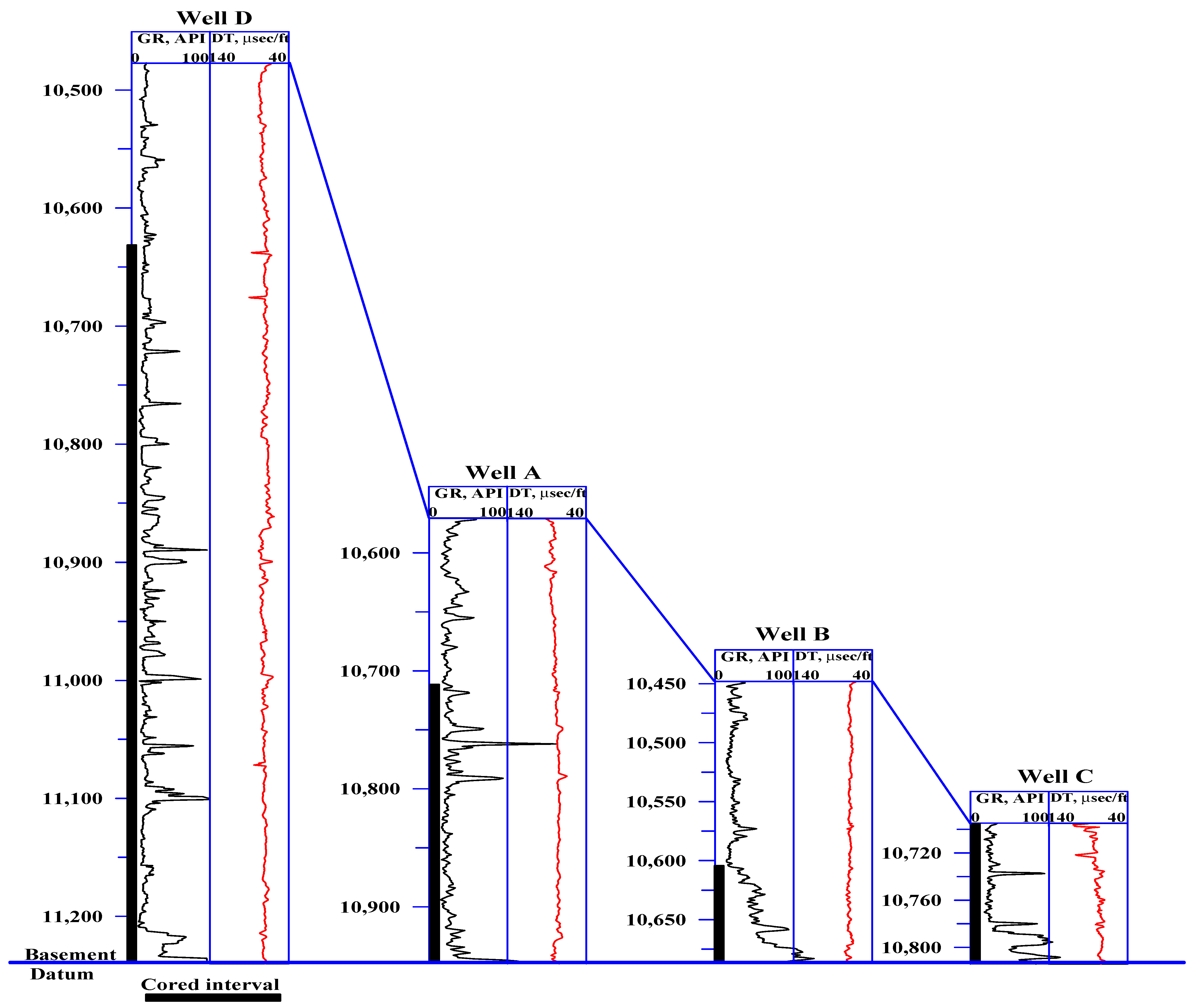
This study used routine core data from seven wells (labeled from A to G), representing different sandstone reservoirs and different geologic ages. The studied wells are located in the southern part of the Gulf of Suez, Egypt. The Gulf of Suez is considered the most prolific hydrocarbon province in Egypt. The Oligocene–Early Miocene Gulf of Suez continental rifting [25] divided the stratigraphic sedimentary history of the Gulf of Suez into two major megasequences: the pre-rift megasequence (which extended from the Cambrian to the Oligocene) and the syn-rift megasequence (Figure 1). Hydrocarbon is delivered from the fractured basement, the pre-rift megasequence interval, and the Miocene syn-rift megasequence. The studied intervals of wells A to D (Figure 2) consist mainly of sandstone intercalated with thin clay layers that range in age from the Cambrian to the Lower Cretaceous. The sandstones are mostly quartz grains, poorly to medium-sorted, and fine- to coarse-cemented. The interval of well E was deposited in the Lower Miocene and consists mainly of sandstone. This sandstone is characterized by very fine to medium grains, with argillaceous cement, traces of mica, pyrite, kaolinite patches, and iron oxide, grading downward into medium to coarse grains, with traces of kaolinite and poorly to medium-cemented grains. The interval of well F was deposited in the Upper Cretaceous. It consists of an intercalation of sandstone and siltstone. The sandstone consists of well-cemented very fine grains, with traces of mica, pyrite, and iron oxide. The interval of well G was deposited in the Middle Miocene. It consists mainly of shale in the upper part, while the lower part is predominantly composed of sandstone. The sandstone is composed of fine to coarse grains, poorly sorted, and medium-cemented, with traces of dolomite. The routine core data include horizontal permeability, helium porosity, and water saturation for a total of 1022 core plug samples. A statistical summary of these data is provided in Table 1.
The general core description indicates that the lithology is sandstone, consisting mainly of quartz grains, ranging from fine- to coarse-grained, subrounded, subangular, medium-sorted, and well-cemented, with kaolinite cement. The permeability distribution is usually, but not always, a log-normal distribution, i.e., ln(k)~(μ, σ2), where μ is the arithmetic mean and σ2 is the variance. Determination of the probability of the permeability distribution is important for determining the proper use of equations in the calculation of heterogeneity measures. Three equations can be utilized to ascertain and verify the distribution of permeability:
1-
For the probability density function of the log-normal distribution (PDF):
f ( x ) = 1 x σ 2 π e x p ( 0.5 ( ( ln x μ ) σ ) 2 )
2-
For the probability density function of the cumulative distribution function (CDF):
f x = 0.5 ( 1 + e r f ( ( ln x μ ) 2 σ )
3-
For the probability density function of the normal distribution:
f ( x ) = 1 σ 2 π e x p ( x μ 2 2 σ 2 )
where x is a random variable—in this study, it is the permeability—σ is the standard deviation, μ is the arithmetic mean, and erf is the error function of (x). Each of these functions has its specific equations to determine the standard deviation and expectation.
Heterogeneity measures can be determined as follows:
The coefficient of variation (CV) is one of the reservoir heterogeneity measures. For a homogeneous reservoir, CV < 0.5, while 0.5 < CV < 1 corresponds to a heterogeneous reservoir, and CV > 1 corresponds to a very heterogeneous reservoir [3]. Therefore, the CV ranges between 0 and ∞. It can be determined from the following equation:
C V = σ 2 E ( x ) = σ μ
where σ2 is the variance and E(x) is the expectation of the random variable (x). For a log-normal distribution, the mean and variance of variable (X) can be determined as follows:
E ( X ) = e x p ( μ + σ 2 2 )
V a r X = exp 2 μ + σ 2 ( exp σ 2 1 )
From Equations (5) and (6), CV can be determined as follows [3]:
C V = σ 2 E ( X ) = exp σ 2 1
The CV can be estimated from the ratio of the permeability arithmetic average (kA) to the permeability harmonic average (kH), as suggested by [4]:
C V = k A k H 1
The Dykstra–Parsons coefficient (VDP) is the most common measure of heterogeneity. It was introduced by [26]. Occasionally, this measure of heterogeneity can be referred to as the coefficient of permeability variation. It takes the following form:
V D P = k 50 - k 84.1 k 50
where VDP is the Dykstra–Parsons coefficient, k50 is the median permeability, and k84.1 is the percentile of a set of permeability data arranged in decreasing order. In simple form:
V D P = x 2 - x 1 x 2
In which,
x 1 = e x p ( μ σ )
x 2 = e x p ( μ )
Alternatively, Equation (9) can be written in the following form when the permeability data are in ascending order:
V D P = 1 - k 0.16 k 0.5
where k0.16 is the percentile from a set of permeability data arranged in increasing order on a log-probability plot. The VDP is zero for homogeneous reservoirs and one for completely (infinitely) heterogeneous ones. According to [3,8], the majority of the drilled reservoirs exhibit VDP values ranging from 0.5 to 0.9. However, Salazar (2018) reported VDP values less than 0.5 for the sandstones of the Little Greek oil field, which were deposited by extremely meandering systems of an upper deltaic plain. Tiab and Donaldson [9] provided a comprehensive classification of heterogeneity of reservoirs based on VDP values, in which:
0 < VDP < 0.25, for slightly heterogeneous,
0.25 < VDP < 0.50, for the heterogeneous reservoir,
0.50 < VDP > 0.75, for a very heterogeneous reservoir,
0.75 < VDP < 1, for an extremely heterogeneous reservoir,
The graphical presentation of VDP has been extensively described in numerous publications, including [8,9,15,22]. In this study, we adopted the procedure provided by [9]). The best-fit straight line that results from plotting cumulative frequency distribution against permeability defines the k50 and k84.1 in descending order and the k0.5 and k0.16 in ascending order.
Schmalz and Rahme [27] used the permeability distribution proposed by [28] to introduce a new heterogeneity measurement. The authors plotted the flow capacity (F) against the cumulative thickness (H) to determine the so-called Lorenz coefficient (Lc) to overcome the drawbacks of the Dykstra–Parsons coefficient. This coefficient is also known as the Gini coefficient [29]. The Lorenz coefficient ranges from 0 for a completely homogeneous reservoir to 1 for a reservoir that is completely heterogeneous. The LC is equal to twice the area between the equality line and the Lorenz curve. Lake [30], Tiab and Donaldson [9], and Salazar [22] proposed a modified Lorenz procedure, in which they utilized the cumulative storage capacity (C) instead of the cumulative thickness, according to the following equations:
F = i = 1 n k i h i i = 1 N k i h i
H = i = 1 N h i i = 1 n h i
C = i = 1 N i h i i = 1 n i i
where 1 ≤ n ≥ N and N is the total number of layers in the reservoir, n is the first to the nth layer considered for the cumulative sum, k is the permeability, and ϕ is the porosity.
Another method that relies on cumulative thickness rather than storage capacity can be found in [15]. Fitch et al. [1] used another Lorenz curve procedure to plot the cumulative storage capacity against the cumulative depth increment. Meanwhile, Mirzaei-Paiaman et al. [31] plotted normalized cumulative porosity against normalized cumulative permeability to determine the Lorenz coefficient.

3. Results

3.1. Data Examination

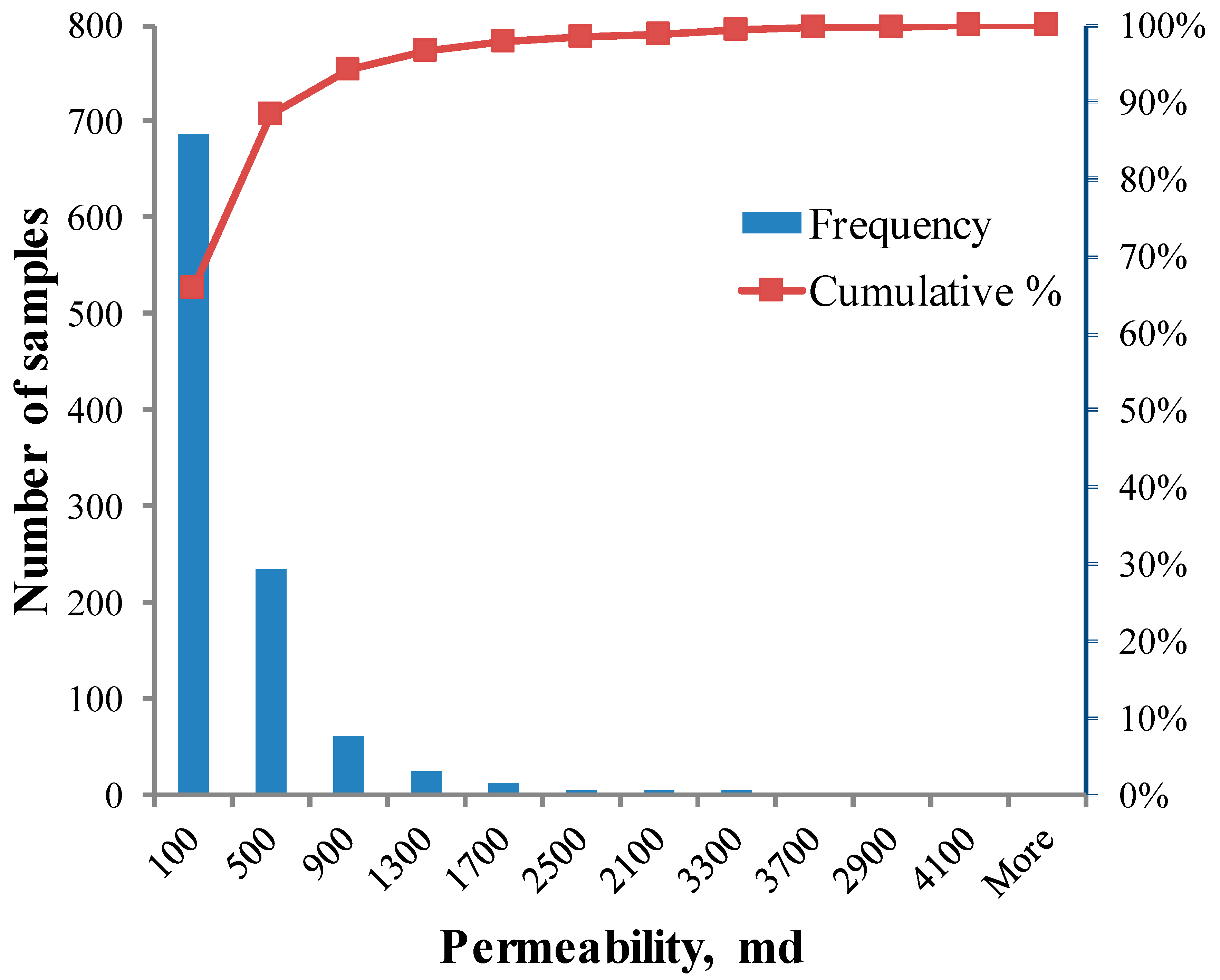
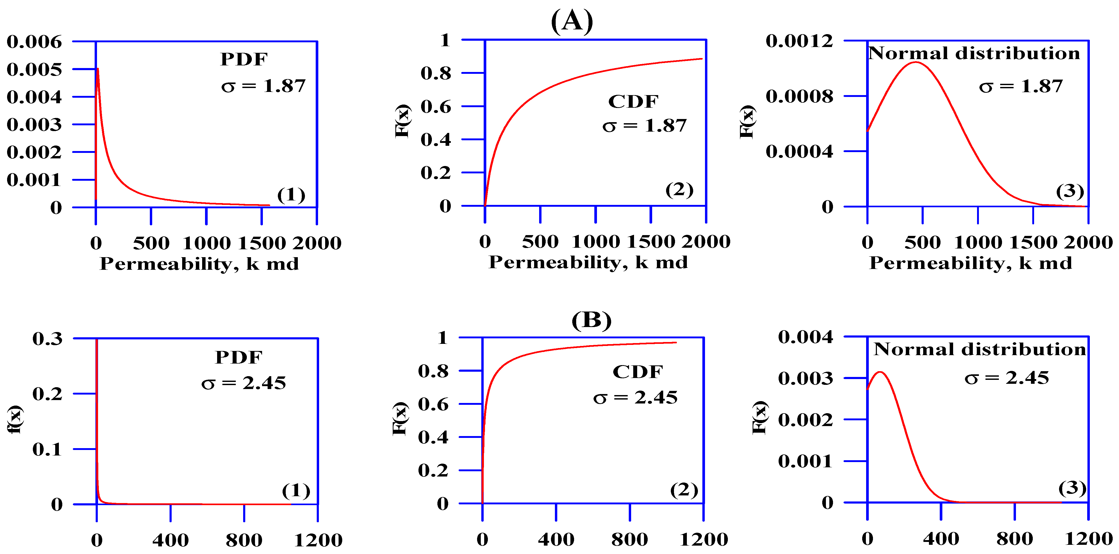
This study used 1022 core plug samples from seven wells with different geological ages (Table 1). The data revealed a wide range of permeability, ranging 0.01 to 4020 md, with an arithmetic average of 212.33 md. The permeability geometric average for all of the data is 20.68 md, whereas the permeability harmonic average is 0.43 md. The pronounced disparity among the three averages suggested heterogeneous reservoirs that could be extremely one. The core porosity ranges from 0.012 to 0.245, with an average value of 0.138. The natural logarithm of permeability has a standard deviation ranging from 1.87 to 3.58 and a mean ranging from 0.8 to 5.33 (Table 2). A histogram can be used to clarify the probability distribution of the permeability data (Figure 3). The log-normal distribution of permeability proposed by [26] for calculating VDP can be verified by applying Equations (1)–(3), as shown in Figure 4. The right tail indicates that the data have a lognormal distribution. It is noteworthy that, with increasing standard deviation, the shape of the PDF changes from its known form (Figure 4). The probability distribution functions show that all the studied wells have log-normally distributed permeability.

3.2. Heterogeneity Measures

Using Equation (4), the CV values ranged from 0.88 to 2.32, indicating heterogeneous to very heterogeneous reservoirs (Table 3). Salazar [22] utilized the standard deviation and mean of the k/ϕ ratio to calculate the CV. Based on his procedure, the values of CV range from 0.86 to 1.98 (Table 3). Notably, the CV calculated via the two methods remained the same for well C. However, all the other wells showed a decrease in the CV values in different amounts, mostly depending on how porous they were (Table 3).
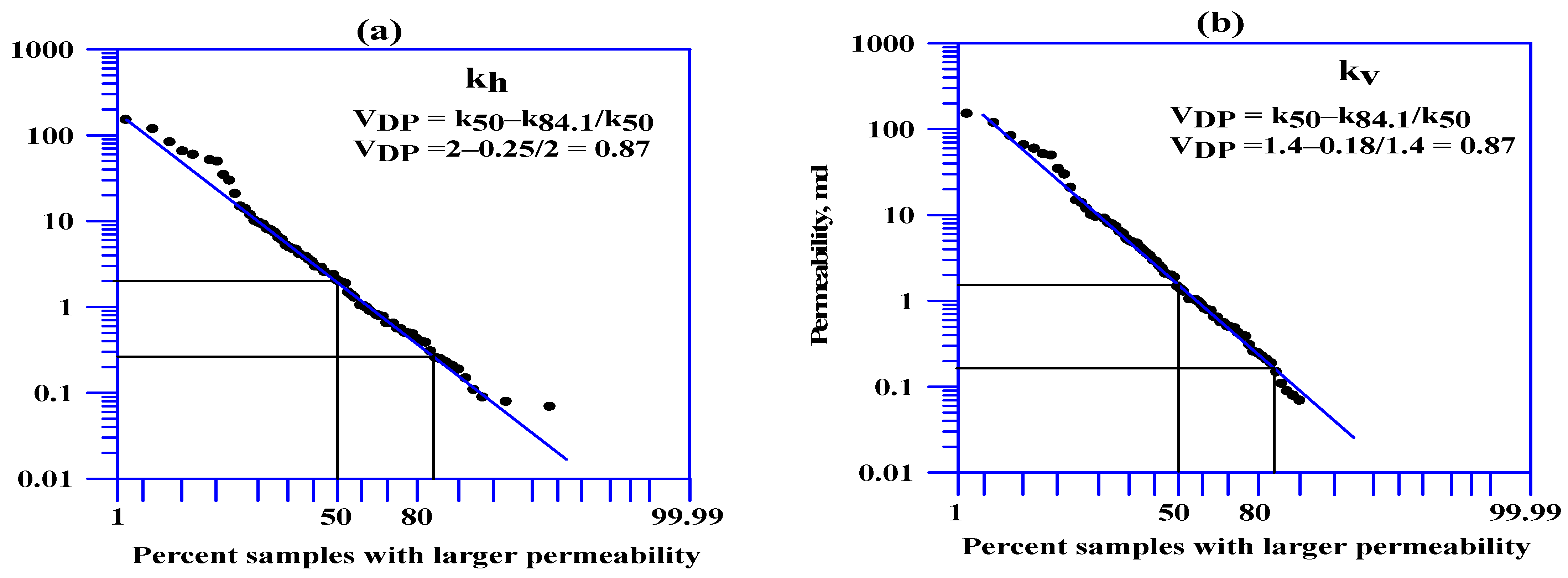
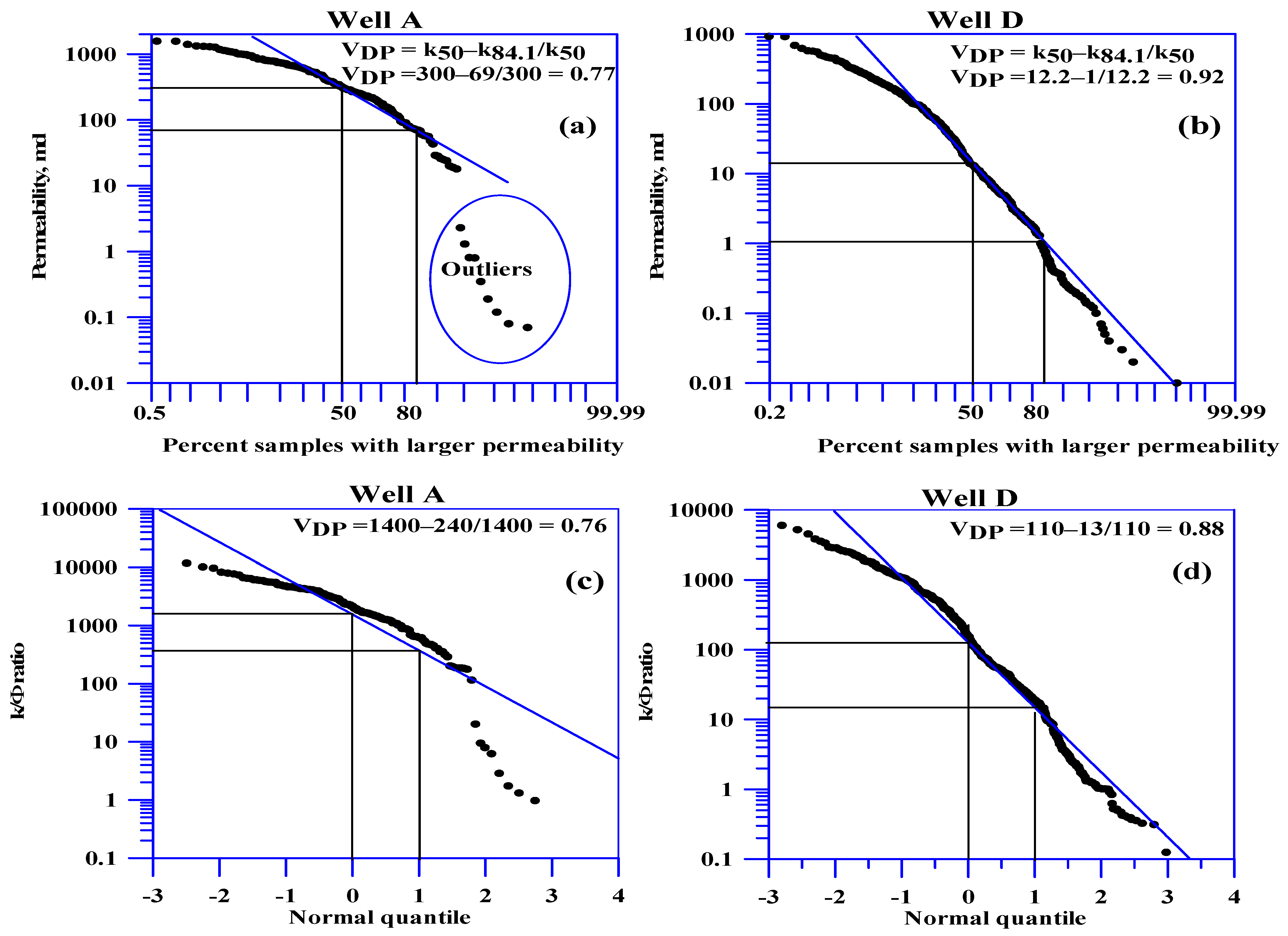
The plot of permeability versus the percentage of samples with larger permeability on a log-probability graph is assumed to be a straight line. A best-fit line can be drawn, and the constraints k50 and k84.1 can be determined (Figure 5). It can be noted that VDP = 0.86 for horizontal permeability, with a slight increase to 0.87 for vertical permeability within this well. Moreover, both plots displayed proficient straight lines (Figure 5). The data yield the identical VDP value (Table 4). Such an ideal case is not often encountered. Figure 6a shows a Dykstra–Parsons plot without an identified straight line. In this case, according to [3], the central points receive more weight than the tail points. Therefore, the VDP for well A is 0.77, which indicates the onset of an extremely heterogeneous reservoir. This technique yielded VDP values comparable to those deduced from the data (Table 4). For Figure 6b, a small variation is observed between the VDP from the plot (=0.92) and that extracted from the permeability data, where VDP = 0.93. Both values indicate an extremely heterogeneous reservoir for this well.
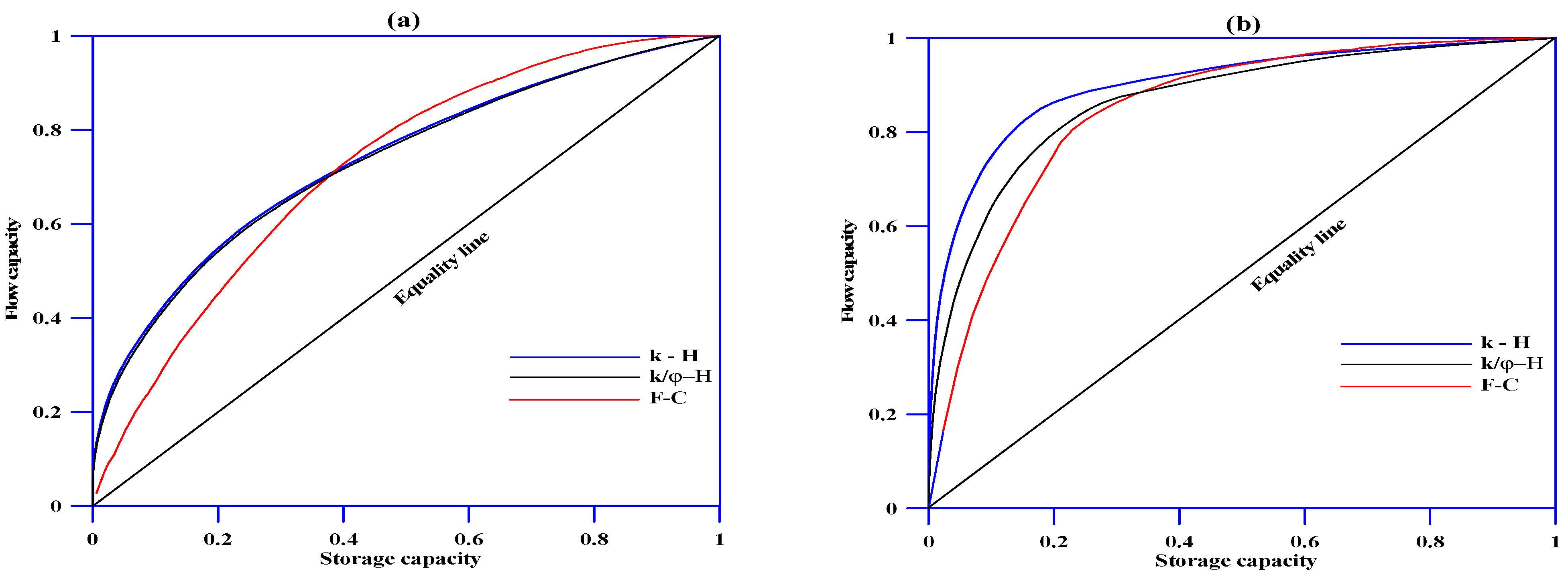
Permeability as a function of thickness can be used to calculate the Lorenz coefficient (LC). In this case, the cumulative thickness frequency is plotted against cumulative permeability to determine the shape of the Lorenz curve and the value of the LC (Figure 7). Table 5 shows the LC values ranging from 0.47 (well A) to 0.8 (well B). Without the division of the LC scale, as with the VDP, the degree of reservoir heterogeneity is obscured.

4. Discussion

4.1. Coefficient of Variation (CV)

Since the permeability data are log-normally distributed, Equation (7) must be used for the calculation. In this case, the CVs recorded very high values, ranging from 5.7 to 597.6, indicating a high degree of heterogeneity (Table 3). These exceptionally high values reflect a high standard deviation. According to [32], the geometric standard deviation (σg) can be used to calculate the CV for log-normal distribution data, in which:
C V = exp { [ ln σ g ] 2 1 }
and,
σ g = 10 σ   o f   l o g   ( k )
Using the geometric standard deviation, the CV values range from 3.46 to 362.45, indicating that the studied reservoirs are very heterogeneous (Table 3). The CV values are still high, but they are lower than the values obtained from Equation (7). These high values of CV could be partly due to the effect of outliers. This effect could be examined for well A. Omission of outliers that are lower than 1 md (8 points), resulted in a reduction of the CV from 3.46 to 1.13. Another example of the effect of outliers is observed in well G. By omitting outliers less than 0.02 md (7 points), the CV was reduced from 362.45 to 63.68. These outcomes align with findings by [33], where the CV is highly affected by the outliers.
The ratio of arithmetic to harmonic averages is another way to calculate the CV. Using Equation (8), the CV values ranged from 4.54 to 38.88, indicating that the reservoirs are very heterogeneous (Table 3). Notably, there was a change in the order of the degree of heterogeneity among reservoirs, which was dominant according to the previous methods (Table 3). As noted, wells C and F had similar and the lowest CV values, in contrast to the previous methods that indicated that well A was the lowest heterogeneous reservoir. This distortion in the heterogeneity order signifies the failure of this method in calculating the CV.
The coefficient of variation can be used to determine the minimum number of samples needed to determine the mean permeability within 20% of the true value. The following equation can be used to determine the number of required samples according to [34]:
N o = 100 C V 2
Equation (19) states that there are insufficient samples to estimate the permeability arithmetic mean when using Equations (7) or (18) to calculate the CV. However, after removing outliers, the CV for well A is 1.13, and the number of required samples = 128. Hence, only well A provided sufficient samples to estimate the permeability arithmetic mean. Nevertheless, Salazar [22] deemed a sample size of 15 as the minimal threshold for estimating heterogeneity measures.
The coefficient of variation is related to the depositional environment of the sediments, where CV < 0.5 is associated with high-energy and well-sorted grains. Conversely, CV > 1 is associated with mixed lithologies, facies, or pore types [34]. The depositional environment, based on the core analysis of well G (CV = 362.45), illustrated that the cored interval was deposited in an open marine environment for the upper mudstone unit, grading to a shallow marine environment with poorly sorted sandstone, occasionally indicating influx from a deltaic source. Although the cored intervals of wells A, B, C, and D consist mainly of sandstone with intercalations of shale deposited in a fluvial braided system and grade to an aeolian environment [35]. These wells have a CV > 1, indicating very heterogeneous reservoirs. The high heterogeneity may be attributed to the presence of different facies, pore types, and clay minerals (mainly kaolinite), with traces of illite and heavy thorium-bearing minerals.

4.2. Dykstra–Parsons (VDP)

The problems associated with Dykstra–Parsons graphical plotting led researchers to calculate VDP based on mathematical equations. For log-normal distribution data, Lake and Jensen [3] stated that VDP can be expressed as a function of the standard deviation. Pintos et al. [36] termed it the theoretical Dykstra–Parsons coefficient:
V D P = 1 E X P ( σ )
Using Equation (20), it can be observed that well A exhibits the greatest variation between the practical and theoretical VDP when compared to the other wells (Table 5). For well A, the value of VDP increases from 0.77 to 0.85. Other wells, on the other hand, showed a decrease in the theoretical values of VDP (wells C–G). Wells A and C revealed significant discrepancies between the practical and theoretical values. Well A recorded a significant increase, and well C recorded a significant decrease. The variation between the graphical plot and the theoretical VDP arises when the plot does not give the expected straight line, as noted for well A (Figure 6a). However, when the best-fit line represents the entire plotting data (as in well B), there is no difference between the plot and the theoretical VDP values (Figure 5). Moreover, when the best-fit line encompasses most of the plotting data (as in well D), the difference between the two values is very small (Figure 6b).
Using the kA/kH ratio proposed by [37], the VDP can be calculated as follows:
V D P = 1 E X P [ L N ( k A k H ) ]
Again, using arithmetic and harmonic averages disrupted the order of the heterogeneity degree of the studied reservoirs (Table 4). Equation (21) results in VDP values lower than those obtained using the standard deviation (Equation (20)). Both equations yield optimistic values when compared to the values obtained from Equation (9) and the data (Table 4). The exception was noted for well A, in which the values were higher than those obtained from Equation (9) and the data.
There were several attempts introduced to modify the Dykstra–Parsons procedure. Based on μ, σ, and ρ, Jensen [17] introduced the following equation to determine VDP:
V D P = 1 [ 1 ρ σ / ( 1 + ρ μ ) ] 1 ρ
Jensen [17] asserted that the exponent ρ is adequate for expressing the tail of the PDF. The exponent ρ is a direct measure of the transformation required to ensure that permeability is normally distributed. The exponent ρ can be estimated from the slope of the following relationship [38]:
y q + y 1 q 2 M ( 1 ρ ) ( y 1 q M ) 2 + ( M y q ) 2 4 M
where yq and yq−1 are the lower and upper qth quantiles, respectively, with median M. Accordingly, ρ is equal to one minus the slope resulting from the plot of the left term on the y-axis and the right term on the x-axis. A log-normal distribution means that ρ = 0 [39]. When ρ = 0 (as in the studied data), Equation (22) is reduced to Equation (20). Another modification was carried out by [18] based on the maximum likelihood technique, in which VDP can be estimated according to the following equations:
V D P M L = 1 E X P ( σ e s t )
In which,
σ e s t = 1 + 0.25 n 1 { 1 n 1 [ ( l o g ( k i ) μ e s t ) ] 2 } 0.5
and
μ e s t = ( 1 n ) l o g ( k i )
where V D P M L is the Dykstra–Parsons coefficient according to the maximum likelihood method, σest is the estimated standard deviation, μest is the estimated mean, n is the number of data points, and k is the permeability. This modification is generally unsuccessful in the studied wells as the modified standard deviation (Equation (25)) yields high values for the majority of wells.
To avoid the log-probability curve proposed by Dykstra–Parsons, Salazar [22] replaced it with a normal quantile to calculate the VDP. He plotted the normal quantile of the cumulative capacity against the k/ϕ. The proposed normal best-fitting line is obtained, and the two percentiles (50th and 16th) are read at 0 and 1 on the x-axis, respectively (Figure 6c,d). The porosity is strongly involved in this procedure. As a consequence, we expect a decrease in VDP and an improvement in the straight line from this method. According to Table 4, the reduction in VDP values was achieved. However, there was no improvement in the assumed straight line (Figure 6c,d). The Dykstra–Parsons and Salazar methods showed significant differences in VDP values for well E, reaching 0.1. It is important to note that this well has the greatest average porosity.
The uncertainty in VDP values has a significant impact on the future planning and development of reservoirs. According to [40], the VDP is considered the most significant parameter influencing vertical sweep efficiency (EV). The EV depends on the permeability variation, mobility ratio (M), and total volume injected. It can be calculated using the Dykstra–Parsons method, which requires the determination of VDP, M, and the WOR (the water-oil ratio expressed in bbl/bbl). Dykstra–Parsons [26] presented graphical charts for different values of the WOR. In this paper, we aim to explain the effect of uncertainty in VDP on calculating cumulative oil production (NP). According to [40], cumulative oil production is a function of the initial oil-in-place (NS) and the recovery factor (R):
N P = N S R
Well E results in VDP values of 0.94 (based on Equation (20)) and 0.86 (based on the quantile method) (Table 4). By analyzing the relative permeability of well E, the mobility ratio was estimated to be 1. Entering values of M and VDP (0.92) at WOR = 25 yielded R (recovery factor) = 0.103. On the contrary, with VDP equal to 0.84, R equals 0.206. Let us assume that the initial oil-in-place (NS) is 12 MMSTB. From Equation (27), NP will equal 1.236 MMSTB (at VDP = 0.92) and 2.472 MMSTB (at VDP = 0.84). Therefore, when the VDP changed from 0.94 to 0.86, cumulative oil production nearly doubled.
The standard error and bias of the estimated VDP can be calculated using the following equations [18]:
S E V D P = 1.486 l o g ( 1 V D P ) ( 1 V D P ) n
m V D P = 0.7488 [ log 1 V D P ] 2 ( 1 V D P ) n
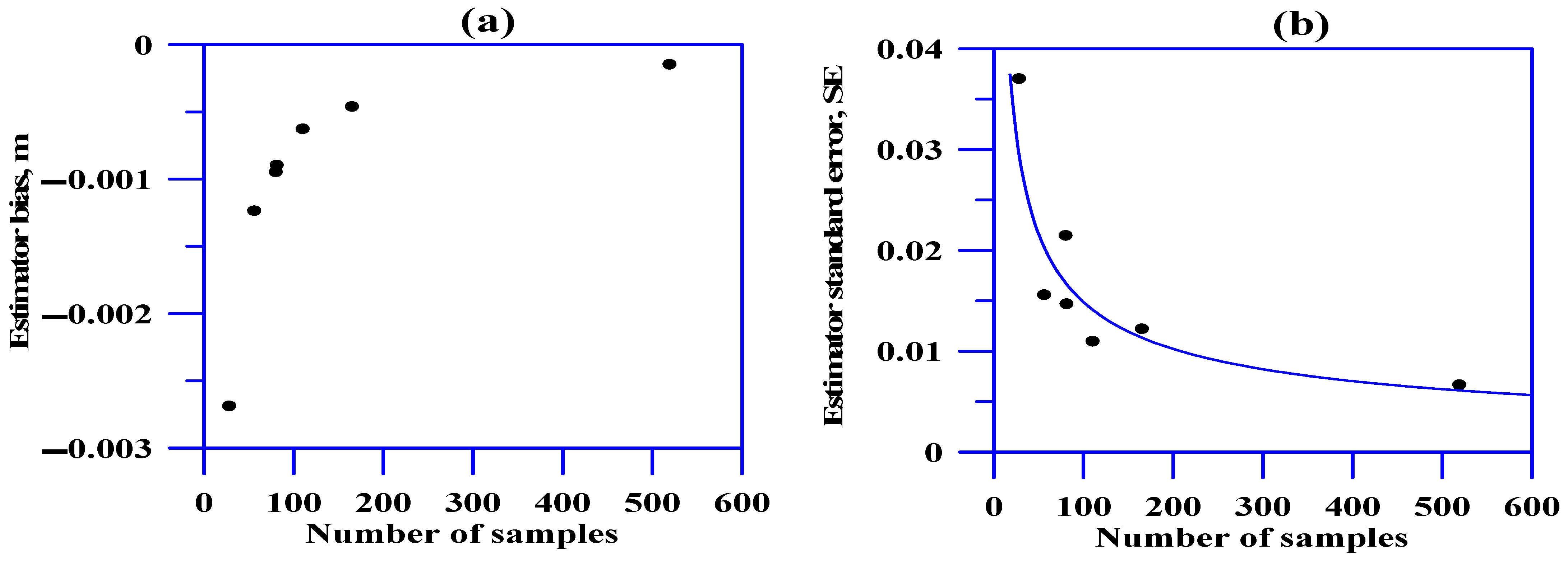
where SEVDP is the standard error of VDP, mvdp is the bias of the VDP, and n is the sample number. Figure 8 shows the relationship between the number of samples and the two parameters. It can be noted that there is an irreversible relationship between the number of samples and the two parameters.

4.3. Lorenz Coefficient, LC

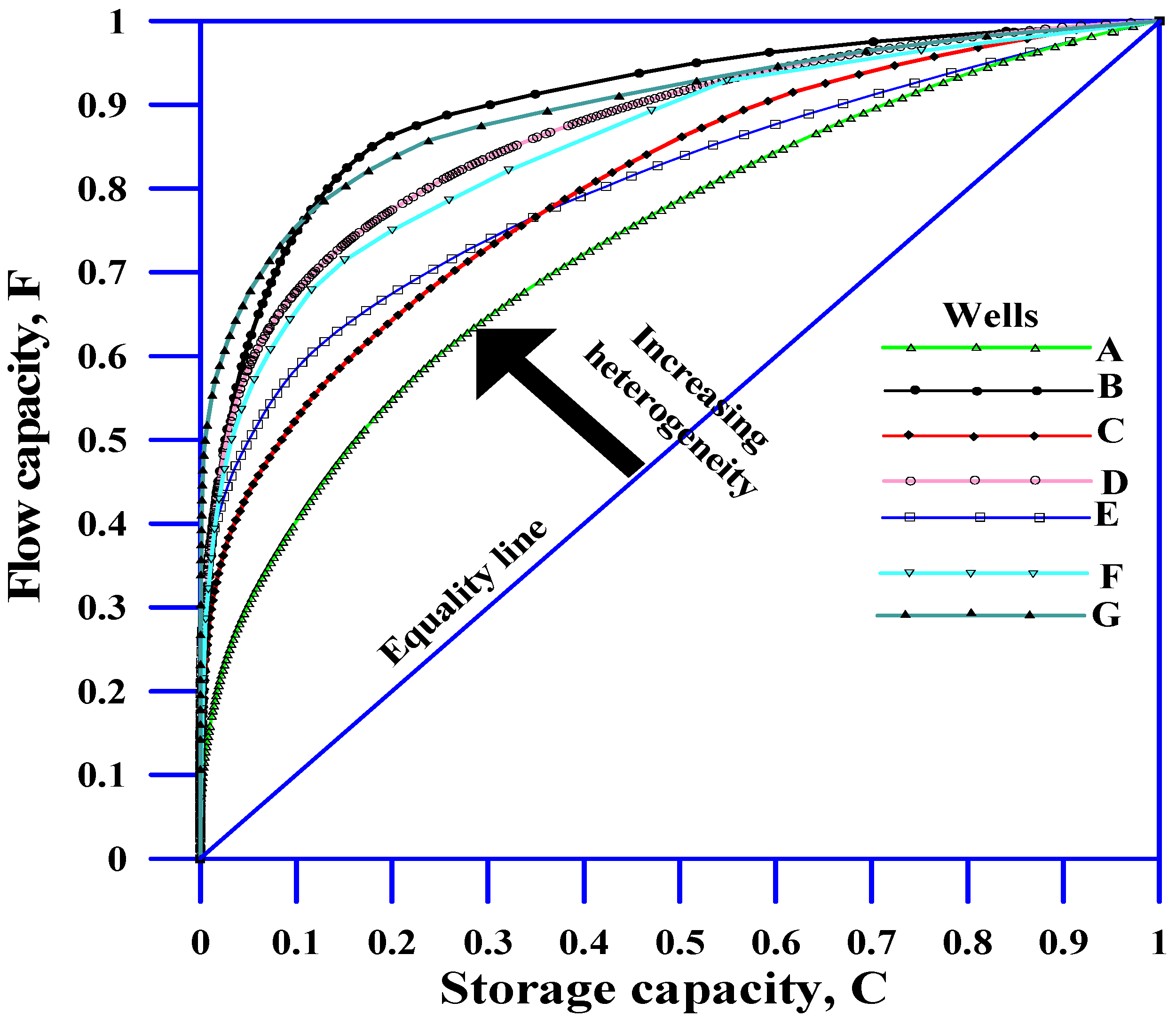
When the k/ϕ ratio was plotted instead of the k, the LC values decreased. The highest average porosity wells—A, C, and E—show little change in LC values, while the lowest average porosity wells—B and F—show more changes in LC values (Table 5). The classical form of the Lorenz curve, in which cumulative storage capacity (C) is plotted against cumulative flow capacity (F), shows a greater decrease in LC values (Figure 9). As expected, a greater decrease is associated with reservoirs with low average porosity (Table 5). Wells E, C, and A recorded the highest average porosities among the studied reservoirs. However, the response of porosity in the determination of LC shows different behaviors. In well A, the LC decreased from 0.47 (calculated from k only) to 0.44 (calculated from C and F). In wells E and C, the LC values decreased from 0.61 and 0.6(calculated from k only) to 0.52 and 0.54 (calculated from C and F), respectively. It is possible that the small effect of porosity in well A is due to the lower heterogeneity of this well compared to wells E and C. Therefore, it can be concluded that the effect of involving porosity in the calculation of LC is not significant for homogeneous to very heterogeneous reservoirs.

4.4. Relationships Between the Heterogeneity Measures

Jensen (1986) related VDP to CV when ρ = 0 (lognormal distribution), where ρ is the transformation exponent in the following equation:
C V = [ ( 1 V D P ) L N 1 V D P 1 ) ] 0.5
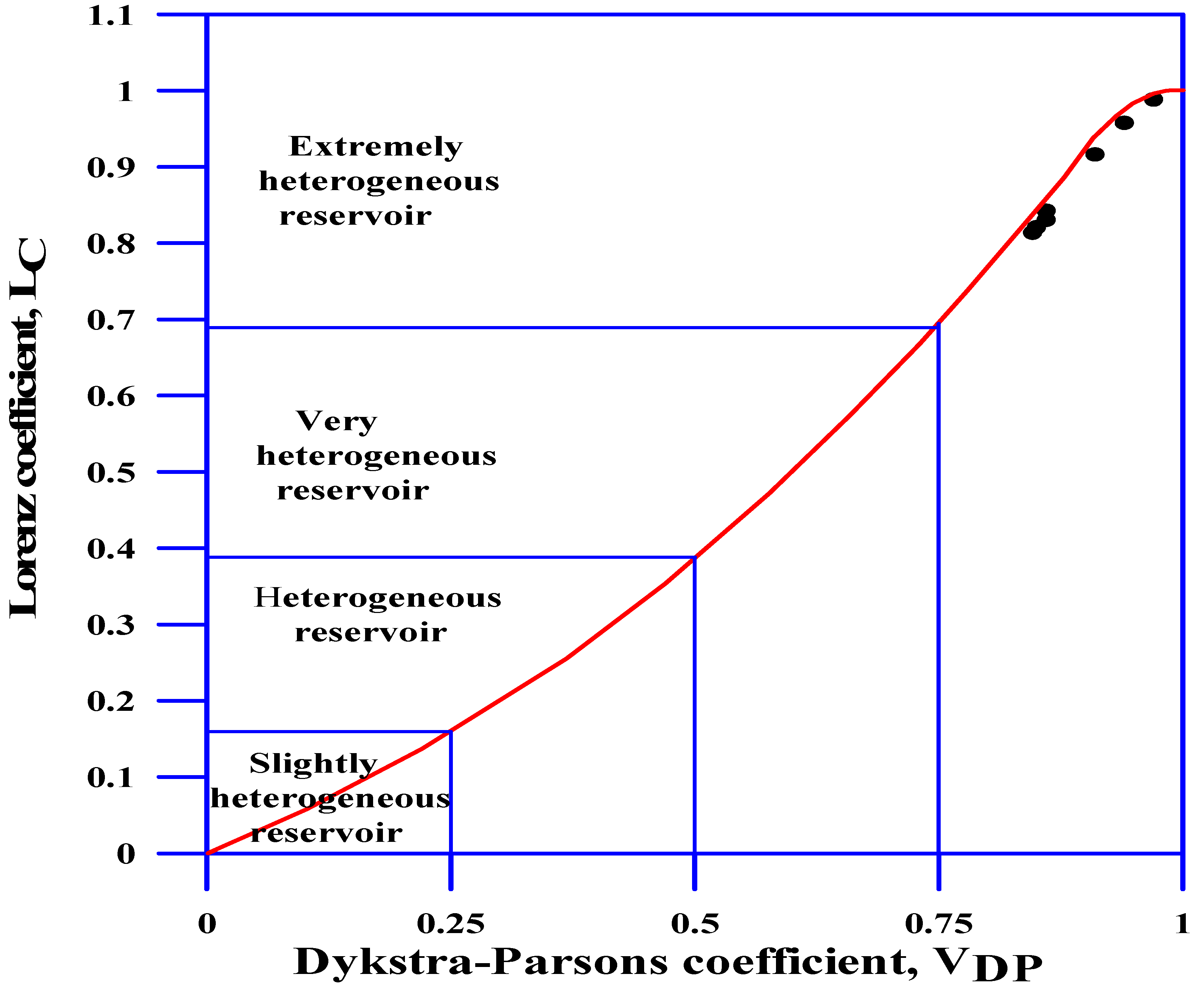
This equation gives CV values similar to those obtained by using Equation (7) (Table 3). Craig [41] presented a graphical plot of the correlation between the Lorenz and Dykstra–Parsons coefficients for log-normal distribution permeability (Figure 10). Based on this plot, Ahmed [40] introduced the following two equations to explain the relationship between VDP and LC:
VDP = −0.000505971 + 1.7475225LC − 1.468855LC2 + 0.701023LC3
L C = 0.0116356 + 0.339794 V D P + 1.066405 V D P 2 0.3852407 V D P 3
For the log-normal permeability distribution, the Lorenz coefficient can be calculated using other heterogeneity measures as follows [4,30]:
L C = e r f ( σ 2 )
L C = e r f [ 0.5 ln 1 V D P ]
L C = e r f [ 0.5 L N 1 + C V 2 ]
According to Equations (33)–(35), a dramatic change in LC values occurred (Table 5). The greatest change was associated with well A, in which the LC changed from 0.47 to 0.81. Furthermore, the least change was associated with well B, where the LC changed from 0.8 to 0.83. It can be concluded that, for any data that show a straight line on the Dykstra–Parsons log-probability plot, VDP and LC can be calculated using any method mentioned in this study. However, for log-normal distribution data with poor straight lines, VDP and LC are suggested to be calculated based on the standard deviation. Depending on the [41] VDP–LC type curve, the LC scale can be divided into the following categories:
0 < LC < 0.16, for slightly heterogeneous,
0.16 < LC < 0.39, for the heterogeneous reservoir,
0.39 < LC > 0.7, for a very heterogeneous reservoir,
0.7 < LC < 1, for an extremely heterogeneous reservoir,
The VDP can be used to calculate the dynamic heterogeneity measure known as the Koval heterogeneity factor (HK), which was introduced by [42]. Koval [43] noted that there is a relationship between the Dykstra–Parsons coefficient and the Koval heterogeneity factor. He expressed this relationship in a type curve. For the log-normal permeability distribution and uniform layers, Paul et al. [43] formulated the following relationship:
l o g ( H K ) = V D P ( 1 V D P ) 0.2
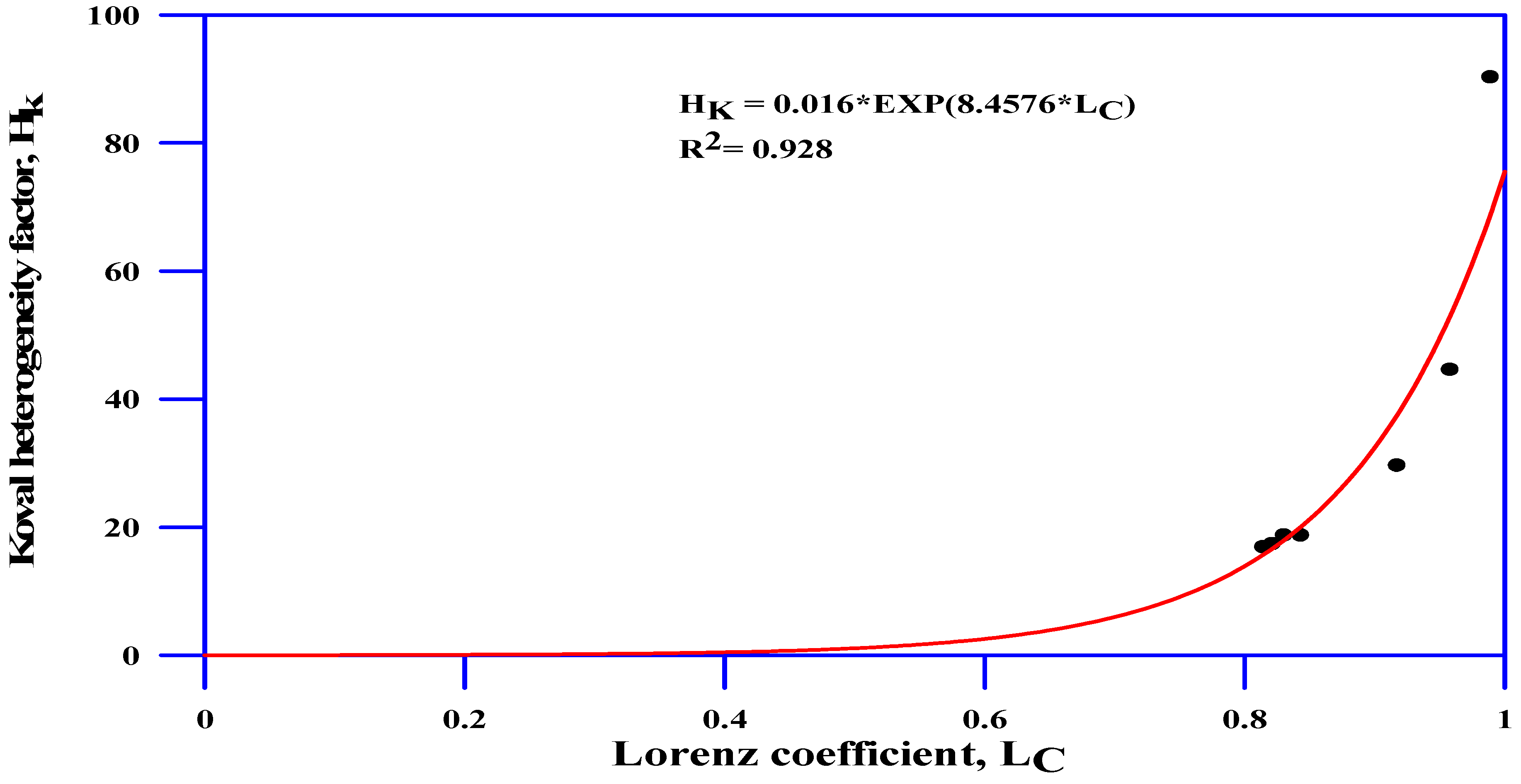
For homogeneous reservoirs, HK equals 1, whereas for heterogeneous reservoirs, there is no upper limit, such as CVs. According to [3], a change in VDP from 0.7 to 0.8 will result in considerable changes in HK. Salazar and Lake [23] plotted ( 1 F ) F vs. ( 1 C ) C in order to estimate HK (Table 5). The HK values of the studied wells indicated the existence of heterogeneous reservoirs, varying in degree. It is noteworthy that there is considerable variation between the Hk values obtained from Equation (36) and those obtained from the plotting of ( 1 F ) F vs. ( 1 C ) C . As expected, the lowest HK value was for well A. However, the highest value was associated with well B. This could be attributed to the role of porosity in the calculation of HK. Well B possesses the lowest average porosity of 0.091. On the other hand, well E possesses the highest average porosity of 0.168. This high average porosity places well B at the second order of the heterogeneity scale among the studied wells. On the contrary, based on Equation (33), the order of heterogeneity degree is similar to that obtained using the theoretical VDP (Table 4). The HK estimated from Equation (36) exhibits a good relationship with the LC (Figure 11). This relationship can be expressed by the following equation, with a coefficient of determination = 0.93:
H K = 0.016 E X P ( 8.4576 L C )
For log-normal distributions, the degree of reservoir heterogeneity for the studied heterogeneity measures can be deduced, as explained in Table 6.

4.5. Relationship Between Heterogeneity and Reservoir Quality

The reservoir quality can be determined using the [12] equation:
R Q I = 0.0314 k
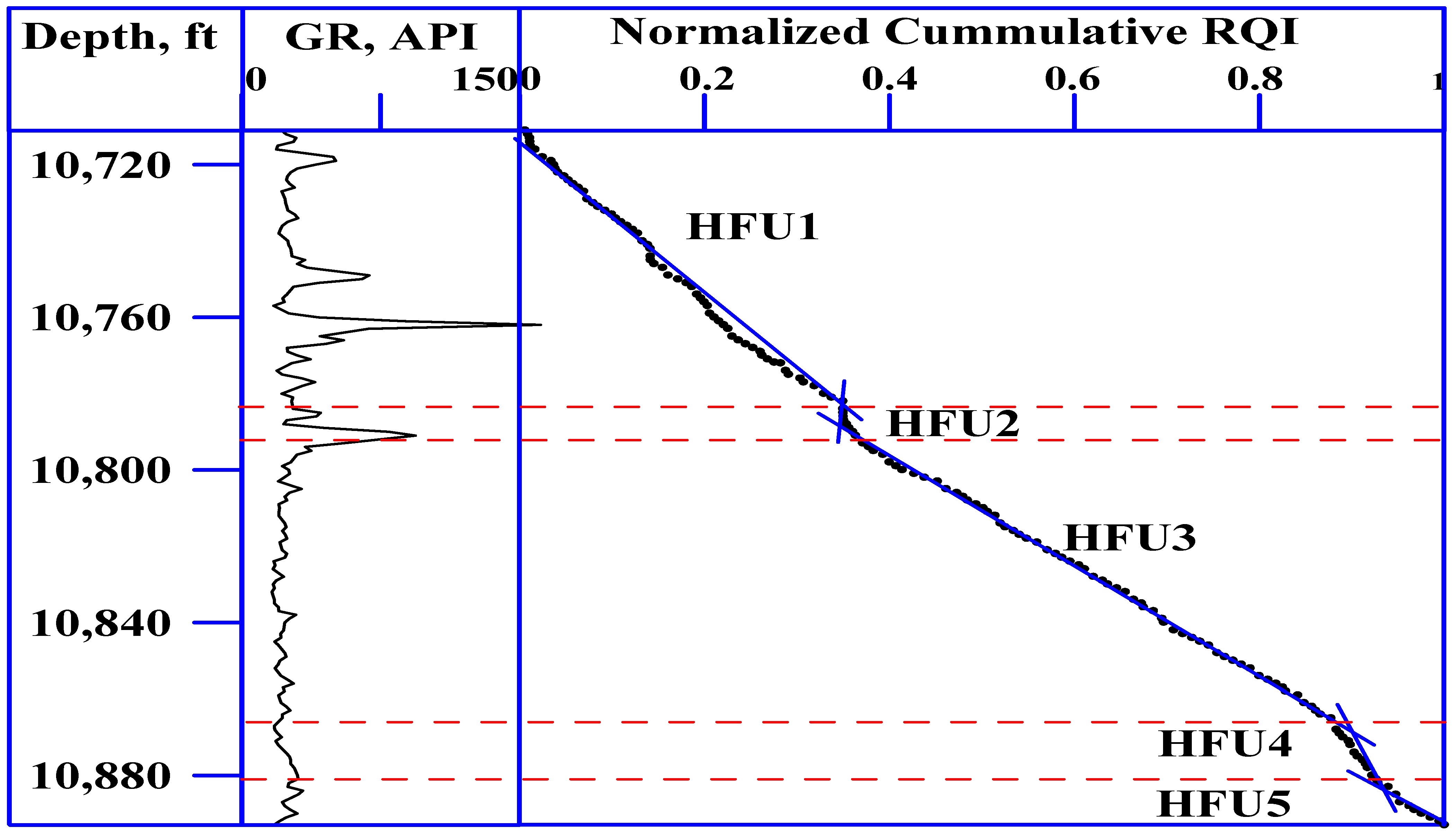
where RQI is the reservoir quality index in microns. To divide the reservoir into flow units, the normalized cumulative reservoir quality index can be calculated and plotted versus depth [44]. There are five hydraulic flow units in well A, which has the least heterogeneous reservoir among the studied wells (Figure 12). The core description indicated a sandstone composed mainly of medium-coarse quartz grains, moderately sorted, and medium-hard, with kaolinite.
For well D, the normalized cumulative reservoir quality index indicated the presence of at least ten hydraulic flow units (Figure 13). Six sandstone lithofacies separated by thin clay layers were identified in the sedimentological core description [45] (Figure 13). Sandstone lithofacies are dark brown, semi-friable, with silicitic cement, conglomerate and argillaceous sandstone, brown sandstone, brown pebbly sandstone, black-colored coarse pebbly sandstone, and white quartzoses plugged by clay minerals. The effect of facies changes was obvious on both the well log responses and the reservoir quality index. The deep resistivity (Rt) log (column 5, Figure 13) is a good indicator of how the reservoir quality changed as sedimentation and diagenesis processes changed. High reservoir quality is associated with high resistivity (Rt > 1000 ohm.m). On the other hand, poor and low reservoir qualities are associated with low resistivity values (Rt < 10 ohm.m). Additionally, the hydraulic flow units mostly reflect the change in the lithofacies.

5. Conclusions

From this study, the following conclusions can be drawn:
  • It is important to define the probability distribution function of permeability in order to determine the proper equations for calculating different heterogeneity measures.
  • The coefficient of variation is strongly affected by the outliers. For log-normal distribution and extremely heterogeneous reservoirs, the coefficient of variation gives high values of three digits
  • In the instance of log-normal distribution data and the absence of straight lines on the Dykstra–Parsons log-probability plot, it is imperative to disregard the VDP values derived from the data and plot, as well as the LC values derived from Lorenz curves. Instead, it is imperative to utilize the VDP and LC calculated based on the standard deviation.
  • For log-normal distribution data with the presence of a straight line on the Dykstra–Parsons log-probability plot, the VDP and LC can be calculated satisfactorily using any method.
  • Modified forms of the Dykstra–Parsons method showed inapplicability in the studied data.
  • The accurate determination of VDP is critical, as decreasing it by 0.08 could result in doubling of cumulative oil production.
  • The inclusion of porosity in the calculation of LC resulted in a decrease in LC values. The percentage of decrease varies depending on the degree of heterogeneity and the average porosity. The effect of porosity decreases in homogeneous to very heterogeneous reservoirs. A tangible effect of porosity was observed in extremely heterogeneous reservoirs with low average porosities.
  • The study introduced a heterogeneity classification for various heterogeneity measures.
  • There is a good correlation between the Lorenz coefficient and the Koval heterogeneity factor.

Funding

This research received no external funding.

Data Availability Statement

The data that support the findings of this study are available from the Egyptian General Petroleum Corporation (EGPC), but restrictions apply to the availability of these data, which were used under license for the current study, and, therefore, are not publicly available. Data are, however, available from the authors upon reasonable request and with permission from the Egyptian General Petroleum Corporation (EGPC).

Acknowledgments

The author is grateful to the Egyptian General Petroleum Corporation (EGPC) and the Gulf of Suez Petroleum Company (GUPCO) for providing the data.

Conflicts of Interest

The author declares that I have no known competing financial interests of personal relationships that could have appeared to influence the work reported in this paper.

References

  1. Fitch, P.J.; Lovell, M.A.; Davies, S.J.; Pritchard, T.; Harvey, P.K. An integrated and quantitative approach to petrophysical heterogeneity. Mar. Pet. Geol. 2015, 63, 82–96. [Google Scholar] [CrossRef]
  2. Tavakoli, V. Carbonate Reservoir Heterogeneity: Overcoming the Challenges; Springer: Berlin/Heidelberg, Germany, 2020; p. 108. [Google Scholar]
  3. Lake, L.W.; Jensen, J.L. A review of heterogeneity measures used in reservoir characterization. In Situ 1991, 15, 409–439. [Google Scholar]
  4. Jensen, J.J.; Lake, L.W.; Corbett, P.W.M.; Goggin, D.J. Statistics for Petroleum Engineers and Geoscientists; Prentice Hall Inc.: New York, NY, USA, 1997; p. 390. [Google Scholar]
  5. Nurmi, R.; Charara, M.; Waterhouse, M.; Park, R. Heterogeneities in carbonate reservoirs: Detection and analysis using borehole electrical imagery. In Geological Applications of Wireline Logs; Hurst, A., Lovell, M.A., Morton, A.C., Eds.; Geological Society Special Publications: London, UK, 1990; Volume 48, pp. 95–111. [Google Scholar]
  6. Frazer, G.W.; Wulder, M.A.; Niemann, K.O. Simulation and quantification of the fine-scale spatial pattern and heterogeneity of forest canopy structure: A lacunarity-based method designed for analysis of Continuous Canopy Heights. For. Ecol. Manag. 2005, 214, 65–90. [Google Scholar] [CrossRef]
  7. Weber, K.J. How heterogeneity affects oil recovery. In Reservoir Characterization; Lake, L.W., Carroll, H.B., Eds.; Academic Press: New York, NY, USA, 1986; pp. 487–544. [Google Scholar]
  8. Willhite, G.P. Waterflooding, 3rd ed.; Society of Petroleum Engineers: Houston, TX, USA, 1986; p. 326. [Google Scholar]
  9. Tiab, D.; Donaldson, E. Petrophysics: Theory and Practice of Measuring Reservoir Rock and Fluid Properties, 3rd ed.; Gulf Publishing Company: Houston, TX, USA, 2012; p. 950. [Google Scholar]
  10. Slatt, R.M.; Galloway, W.E. Geological heterogeneities. In Development Geology Manual Reference; Morton-Thompson, D., Woods, A.M., Eds.; AAPG: Tulsa, OK, USA, 1992; pp. 278–281. [Google Scholar]
  11. Winland, H.D. Oil accumulation in response to pore size changes, Weyburn field, Saskatchewan. In Amoco Production Research Report; Scientific Research Publishing Inc.: Wuhan, China, 1972; p. F72-G-25. [Google Scholar]
  12. Amaefule, J.O.; Altunbay, M.; Tiab, D.; Kersey, D.G.; Keelan, D.K. Enhanced reservoir description: Using core and log data to identify hydraulic (flow) units and predict permeability in uncored intervals/wells. In Proceedings of the 68th Annual Technical Conference and Exhibition, Houston, TX, USA, 3–6 October 1993; p. 16. [Google Scholar]
  13. Gunter, G.; Finneran, J.; Hartmann, D.; Miller, J. Early determination of reservoir flow units using an integrated petrophysical method. In Proceedings of the SPE Annual Technical Conference and Exhibition, San Antonio, TX, USA, 5–8 October 1997; p. 8. [Google Scholar]
  14. Lucia, F.J. Rock fabric/petrophysical classification of carbonate pore space for reservoir characterization. AAPG Bull. 1995, 79, 1275–1300. [Google Scholar]
  15. Smith, J.T.; Cobb, W.M. Waterflooding; Midwest Office of the Petroleum Technology Transfer Council: Oak Hill, VA, USA, 1997. [Google Scholar]
  16. Miller, M.G.; Lents, M.R. Performance of Bodcaw Reservoir, Cotton Valley Field Cycling Project: New Methods of Predicting Gas-Condensate Reservoir Performance Under Cycling Operations Compared to Field Data; American Petroleum Institute: Washington, DC, USA, 1946; API-46-128. [Google Scholar]
  17. Jensen, J.L. A Statistical Study of Reservoir Permeability Distributions. Ph.D. Thesis, The University of Texas at Austin, Austin, TX, USA, 1986; p. 234. [Google Scholar]
  18. Jensen, J.L.; Currie, I.D. New method for estimating the Dykstra-Parsons coefficient to characterize reservoir heterogeneity. SPE Reserv. Eng. 1990, 5, 369–374. [Google Scholar] [CrossRef]
  19. Nyvoll, A. Correlating Recovery Factors with Measures of Reservoir Heterogeneity. Master’s Thesis, Norwegian University of Science and Technology, Trondheim, Norway, 2008; p. 118. [Google Scholar]
  20. Jing, W.; Huiqing, L.; Zenglin, W. Quantitative models of development laws for heterogeneous sandstone reservoirs by water flooding. Open Pet. Eng. J. 2012, 5, 26–35. [Google Scholar] [CrossRef]
  21. Canchola, A.; A Canchola, S.T.J.; Hemyari, E.P.P.; Marins, E. Correct Use of Percent Coefficient of Variation (%CV) Formula for Log-Transformed Data. MOJ Proteom. Bioinform. 2017, 6, 316–317. [Google Scholar] [CrossRef]
  22. Salazar, J.J. Heterogeneity Study of the Little Creek Field from Petrophysical Data. Master’s Thesis, The University of Texas at Austin, Austin, TX, USA, 2018; p. 134. [Google Scholar]
  23. Salazar, J.J.; Lake, L.W. The physical meaning of the Koval factor. Math. Geosci. 2020, 52, 1017–1033. [Google Scholar] [CrossRef]
  24. Ren, B.; Jensen, J.; Lake, L.; Duncan, I.; Male, F. Analysis of vertical permeability and its influence on CO2 enhanced oil recovery and storage in a carbonate reservoir. In Proceedings of the Annual Technical Conference and Exhibition, Dubai, United Arab Emirates, 21–23 September 2021. [Google Scholar]
  25. Patton, T.L.; Moustafa, A.R.; Nelson, R.A.; Abdine, A.S. Tectonic evolution and structural setting of the Suez rift. In Interior Rift Basins; Landon, S.M., Ed.; AAPG: Tulsa, OK, USA, 1994; pp. 9–55. [Google Scholar]
  26. Dykstra, H.; Parsons, R.L. The prediction of oil recovery by waterflood. In Secondary Recovery of Oil in the United States: Principles and Practice; American Petroleum Institute: Washington, DC, USA, 1950; pp. 160–174. [Google Scholar]
  27. Schmalz, J.P.; Rahme, H.D. The variation of waterflood performance with variation in permeability profile. Prod. Mon. 1950, 15, 9–12. [Google Scholar]
  28. Stiles, W.E. Use of permeability distribution in water flood calculations. Trans. AIME 1949, 186, 9–13. [Google Scholar] [CrossRef]
  29. Kendall, M.; Stuart, A. The Advanced Theory of Statistics, Vol. 1: Distribution Theory, 4th ed.; MacMillian Publishing Co.: New York, NY, USA, 1977; p. 472. [Google Scholar]
  30. Lake, J.W. Enhanced Oil Recovery; Prentice Hall Inc.: Upper Saddle River, NJ, USA, 1989; p. 550. [Google Scholar]
  31. Mirzaei-Paiaman, A.; Asadolahpour, S.R.; Saboorian-Jooybari, H.; Chen, Z.; Ostadhassan, M. A new framework for selection of representative samples for special core analysis. Pet. Res. 2020, 5, 210–226. [Google Scholar] [CrossRef]
  32. Von Sperling, M.; Verbyla, M.E.; Oliveira, M.A.C. Assessment of Treatment Plant Performance and Water Quality Data: A Guide for Students, Researchers and Practitioners; IWA Publishing: London, UK, 2020; p. 644. [Google Scholar]
  33. Kvalseth, T.O. Coefficient of variation: The second-order alternative. J. Appl. Stat. 2016, 44, 402–415. [Google Scholar] [CrossRef]
  34. Corbett, P.; Jensen, J. Estimating the mean permeability: How many measurements do you need? First Break 1992, 10, 89–94. [Google Scholar] [CrossRef]
  35. El Sharawy, M.S.; Gaafar, G.R. Reservoir zonation based on statistical analyses: A case study of the Nubian sandstone, Gulf of Suez, Egypt. J. Afr. Earth Sci. 2016, 124, 199–210. [Google Scholar] [CrossRef]
  36. Pintos, S.; Bohorquez, C.; Queipo, N.V. Asymptotic Dykstra–Parsons distribution, estimates and confidence intervals. Math. Geosci. 2011, 43, 329–343. [Google Scholar] [CrossRef]
  37. Tarhuni, M.N.; Sulaiman, W.R.; Jaafar, M.Z.; Sabil, K.M. A novel energy lifting approach using J-function and flow zone indicator for oil fields. Energy Eng. 2022, 119, 253–273. [Google Scholar] [CrossRef]
  38. Emerson, J.D.; Stoto, M.A. Exploratory methods for choosing power transformations. J. Am. Stat. Assoc. 1982, 77, 103–108. [Google Scholar] [CrossRef]
  39. Jensen, J.L.; Hinkley, D.V.; Lake, L.W. A Statistical Study of Reservoir Permeability: Distributions, Correlations and Averages. SPE Form. Eval. 1987, 2, 461–468. [Google Scholar] [CrossRef]
  40. Ahmed, T. Reservoir Engineering Handbook, 4th ed.; Gulf Professional Publishing: Houston, TX, USA, 2010; p. 1454. [Google Scholar]
  41. Craig, F.F. The Reservoir Engineering Aspects of Waterflooding, 2nd ed.; Society of Petroleum Engineers: Dallas, TX, USA, 1971; p. 134. [Google Scholar]
  42. Koval, E.J. A method for predicting the performance of unstable miscible misplacement in heterogeneous media. Soceity Pet. Eng. J. 1963, 3, 145–154. [Google Scholar] [CrossRef]
  43. Paul, G.W.; Lake, L.W.; Pope, G.A.; Young, G.B. A simplified predictive model for micellar-polymer flooding. In Proceeding of the SPE California Regional Meeting, San Francisco, CA, USA, 24–26 March 1982. [Google Scholar] [CrossRef]
  44. Siddiqui, S.; Okasha, M.T.M.; Funk, J.J.; Al-Harbi, A.M. New representative sample selection criteria for special core analysis. In Proceedings of the International Symposium of the Society of Core Analysts, Pau, France, 21–24 September 2003; p. 11. [Google Scholar]
  45. Gameel; Darwish, M. Reservoir behavior of the Pre-Turonian sandstones in south Gulf of Suez province (Sidki field—Case history). In Proceedings of the 12th EGPC Exploration and Production Conference, Cairo, Eegypt, 12–15 November 1994; Volume 2, pp. 449–471. [Google Scholar]
Figure 1. Generalized stratigraphic column of the southern Gulf of Suez. The ages of the formations is adopted from [25].
Geosciences 15 00098 g001
Figure 2. Well–well correlation showing the cored interval of the same rock unit in wells A, B, C, and D.
Geosciences 15 00098 g002
Figure 3. Histogram showing the permeability distribution in the studied wells.
Geosciences 15 00098 g003
Figure 4. Lognormal distribution of the permeability data in the studied wells. (A): Low standard deviation shows the known response with PDF. (B): The high standard deviation shows a different shape of the PDF. In both cases, the right tail demonstrates the log-normal distribution.
Geosciences 15 00098 g004
Figure 5. Dykstra–Parsons on the log-normal probability plot for well B. (a) Horizontal permeability (kh). (b) Vertical permeability (kv).
Geosciences 15 00098 g005
Figure 6. Dykstra–Parsons on the log-normal probability plot for wells A and D (a,b). Both were more weighted toward the central points rather than the extremities. The normal quantile [22] for the same wells (c,d) shows no improvement in the shape of the proposed straight line from the plotted data.
Geosciences 15 00098 g006
Figure 7. Lorenz curves based on different methods for (a) well A and (b) well B. The effect of porosity is evident in well B.
Geosciences 15 00098 g007
Figure 8. (a) Number of samples versus estimator bias; (b) number of samples versus estimator standard error.
Geosciences 15 00098 g008
Figure 9. Order of heterogeneity as deduced from the Lorenz curves for all studied wells.
Geosciences 15 00098 g009
Figure 10. Relationship between Dykstra–Parsons and Lorenz coefficients for log-normal distribution data (modified after [41]). Based on this plot, the LC scale can be divided into different heterogeneity degrees.
Geosciences 15 00098 g010
Figure 11. Good correlation between the Lorenz (LC) coefficient and the Koval heterogeneity factor (HK).
Geosciences 15 00098 g011
Figure 12. Normalized cumulative reservoir quality index versus depth for well A, indicating the presence of five hydraulic flow units.
Geosciences 15 00098 g012
Figure 13. Normalized cumulative reservoir quality index versus depth for well D, indicating the presence of at least ten hydraulic flow units.
Geosciences 15 00098 g013
Table 1. Statistical summary of the horizontal permeability data used.
WellNo. of SamplePermeability, md
St.devMin.Max.kAkHkGkA/kH
A164381.90.071960435.63.44206.8126.6
B8031.960.0717713.770.5422.2225.4
C94259.470.46216101989.1764.7821.59
D519126.650.01105068.080.41310.93164.8
E8111760.0840201035.771.996177.88517.9
F2814.220.07608.630.3991.9321.6
G562110.011072106.390.074.491519.9
Total1022
St.dev = standard deviation, kA = arithmetic mean, kH = harmonic mean, kG = geometric mean.
Table 2. Values of standard deviation and mean of the natural logarithm of permeability (lnk).
WellSt.dev. (σ) of ln kMean (μ) of ln k
A1.875.33
B1.940.8
C1.94.17
D2.452.39
E2.875.18
F20.66
G3.581.5
Table 3. Values of the coefficient of variation (CV).
WellPHI Avg.Coefficient of Variation (CV)
Equation (4)SalazarEquation (7)Equation (8)Equation (17)Equation (30)
A0.1610.880.865.6511.273.465.67
B0.0912.321.986.544.944.016.84
C0.1631.311.315.994.543.825.96
D0.1331.861.719.912.812.0918.13
E0.1681.141.162.1622.7637.752.32
F0.0991.651.357.314.544.476.84
G0.1201.981.93597.638.88362.45467.77
Table 4. Values of the Dykstra–Parsons coefficient (VDP) and the Koval heterogeneity factor (HK).
WellDykstra–Parsons Coefficient (VDP)HK
VDP PlotVDP DataEquation (20)Equation (21)QuantileEquation (31)HK PlotEquation (36)
A0.770.770.8460.890.760.563.217
B0.860.860.860.830.850.828.718.8
C0.950.950.850.930.810.71517.5
D0.920.930.910.90.880.777.829.7
E0.990.990.940.920.860.674.144.7
F0.930.920.860.830.80.745.318.8
G0.990.990.970.930.9450.815.190.3
Table 5. Values of the Lorenz coefficient (LC).
WellPHI Avg.Lorenz Coefficient (LC)
k-Hk/phi-HF-CEquation (32)Equation (33)Equation (34)Equation (35)
A0.1610.470.460.440.830.810.810.81
B0.0910.800.740.700.850.830.840.83
C0.1630.60.590.540.830.820.820.82
D0.1330.740.710.680.910.920.910.92
E0.1680.610.590.520.950.960.950.96
F0.0990.710.650.600.850.840.840.84
G0.1200.790.770.660.990.990.990.99
Table 6. Heterogeneity degree according to various heterogeneity measures for log-normal distribution data.
Heterogeneity
Measures
HomogeneousSlightly
Heterogeneity
HeterogeneityVery
Heterogeneity
Extremely
Heterogeneity
More ThanLess ThanMore ThanLess ThanMore ThanLess ThanMore ThanLess Than
CV00.0.290.290.790.792.4>2.4
VDP000.250.250.50.50.750.751
LC000.160.160.380.380.670.671
HK111.841.843.753.759.75>9.75
Disclaimer/Publisher’s Note: The statements, opinions and data contained in all publications are solely those of the individual author(s) and contributor(s) and not of MDPI and/or the editor(s). MDPI and/or the editor(s) disclaim responsibility for any injury to people or property resulting from any ideas, methods, instructions or products referred to in the content.