Spatial Variability in Geotechnical Properties Within Heterogeneous Lignite Mine Spoils

Featured Application

This work can be applied to coal (hard coal and lignite) spoil heaps, particularly during decarbonization and in the post-coal era. Former coal mining sites are being reclaimed, with spoil heaps covering large areas that are difficult to valorize. The appropriate and sustainable exploitation of these areas depends directly on their geotechnical analysis. Advanced numerical and stochastic tools appear to be the most suitable method for the robust geotechnical design of these highly heterogeneous spoil materials, making this advanced characterization an essential basis.

Abstract

During surface coal mining, vast amounts of overburden waste materials—called spoils—are excavated and dumped, forming massive heaps, the sustainable exploitation of which is a top priority globally. This study addresses the advanced geotechnical characterization of spoil materials, focusing on lignite mine spoil heaps, which are often ignored due to their highly heterogeneous nature. This research quantifies the spatial variability in spoil materials from a large heap in Greece, highlighting the importance of a robust geotechnical framework for their effective reclamation. Using statistical analysis and variogram modeling, the scale of fluctuation (SoF) was derived for both the vertical and horizontal directions. The SoF values for spoil properties are found to be on the high end of the natural soil range. Vertical correlations are observed for distances over 10 m, occasionally reaching 20 m, indicating significant spatial variability; in the horizontal direction, the SoF reaches up to 285 m. These findings suggest that spoil elements exhibit important spatial dependence, which is critical for their proper design and exploitation. The results provide a basis for future research and the use of advanced numerical tools, such as the random finite element method, to support geotechnical design and the sustainable exploitation of spoil heaps.

1. Introduction

Coal (hard coal and lignite) has historically played a key role in meeting global energy demands. However, the growing efforts for transition to cleaner energy forms in Europe and worldwide to combat climate change have driven a significant transformation in the coal industry and the coal regions dependent on it. As coal mines are closing in a direct response to commitments to reduce CO₂ emissions, coal regions have become particularly vulnerable, needing innovative economic plans, the reclamation of depleted mining areas, and financial and practical support. Policies such as the European Green Deal aim to support these regions by promoting sustainable development, economic diversification, and land rehabilitation. Amid these challenges lies a critical element that has long been neglected and underutilized: spoil heaps. Global coal production has remained significant, e.g., with major coal producers collectively producing over 7 billion tons annually [1]. With the typical stripping ratios for surface coal mining ranging from 2:1 to 10:1, several tons of spoil material are generated for every ton of coal extracted. Over the last 30 years, the cumulative amount of overburden waste has reached trillions of cubic meters, forming extensive spoil heaps.

These massive piles of excavated materials, originally overburden to coal seams, have been typically dumped with little or no concern for future reuse, reclamation, or valorization. Nowadays, spoil heaps are emerging as the key elements in the reclamation of mining landscapes and the broader transition to a post-mining economy. Their potential, however, remains largely unexploited due to various reasons, some of which relate to their geotechnical properties and behavior. The exploitation of spoil heaps has largely been limited to agriculture and forestry with low-load structural systems that reduce the engineering challenges. Μore efficient reclamation techniques have been proposed; however, if one is examining the use of heaps to install photovoltaic cells, heat pumps, and wind turbines, then settlement and stability issues arise. The nature of spoil material characterizes these challenges, and as a result, the more rigorous and accurate characterization of spoil materials is needed.

Due to the often chaotic nature of spoils, their characterization is challenging, and the engineering design of efficient solutions is demanding. Spoils are usually considered as one material with significant uncertainty. The geotechnical properties of several European lignite mine spoil heaps have been analyzed in the past [2], concluding that they present huge variability, far more significant than that of natural soils. It has also been underlined that spoil heterogeneity is highly affected by the transportation and dumping methods, the different origins of soils, and the duration and time planning of different construction stages [3]. One main barrier to the appropriate valorization of spoil heaps remains the challenges posed by the heterogeneous nature of spoil materials [2,4,5,6], and thus there have been attempts to overcome this issue in a probabilistic way [7,8].

The conventional tools for dealing with soil uncertainty and heterogeneity are high safety factors and empirical knowledge mainly related to geotechnical failures. Nevertheless, statistical analysis and stochastic processes are the leading and most efficient ways to address the significant geotechnical uncertainties related to spoil properties. Statistical distributions have been a handy tool to quantify geotechnical uncertainty and soil heterogeneity [9,10,11,12]. A more advanced way to analyze and simulate the heterogeneity of spoil materials is by describing spatial variability. Several researchers have quantified the effects of spatial variability in geotechnical engineering applications for shallow and deep foundations [13], slope stability [14], retaining walls [15], seepage [16], and even soil elastic properties [17]. Furthermore, several researchers have analyzed the spatial variability in soils, e.g., the scale of fluctuation in sands based on CPT data were analyzed in previous works ([18,19]).

The systematic geotechnical characterization of spoil materials remains scarce in the literature. However, recent studies have advanced the understanding of spoil geotechnical properties. Two existing works conducted detailed assessments of lignite mine waste dump materials using Cone Penetration Tests (CPTs), providing foundational insights into spatial heterogeneity and fluctuation scales in such deposits [20,21]. These works successfully applied the random field theory to quantify spoil materials’ variability and introduced stochastic approaches to quantify uncertainty. Despite these advancements, challenges persist in the spatial characterization of spoil materials. Additionally previous research further highlighted that dump soil exhibits substantial differences in consistency, density, and mechanical properties due to excavation, transport, and dumping processes, and statistically (but not spatially) analyzed it ([22]). These factors introduce complexities in geotechnical modeling and stability assessments. In parallel, research has explored the UAV-based monitoring of spoil piles, demonstrating the potential and effectiveness of high-resolution remote sensing techniques for spatial characterization [23]. Finally previous research has presented a promising approach (phytostabilization) for managing spoil material instability [24], particularly in coal mine overburden dumps. In this work, the authors underlined the importance of probabilistic and statistical analyses for spoil materials.

The recent analysis of spoil geotechnical properties [3], complemented by their probabilistic characterization [25], serves as the foundational step for this study. To address the challenge of significant inhomogeneity, spatial characterization and stochastic analysis appear to be the only systematic approaches. However, no prior research has examined the spatial variability in spoil materials’ geotechnical properties in a way that allows its integration into such analyses.

This study seeks to fill this critical gap by conducting the advanced statistical analysis of lignite spoil materials and quantifying spatial variability within a large spoil heap. The examined massive spoil heap’s geotechnical parameters [6] are systematically analyzed using well-established methods (i.e., variogram modeling), revealing spatial variability. The results of this work (statistical distributions and spatial characteristics) can be directly used for the stochastic analysis of spoil materials. The robust geotechnical design of spoil heaps would require the use of advanced numerical tools (e.g., the random finite element method), making the present advanced geotechnical characterization a necessary basis.

2. Study Area and Methods for Spatial Variability Quantification

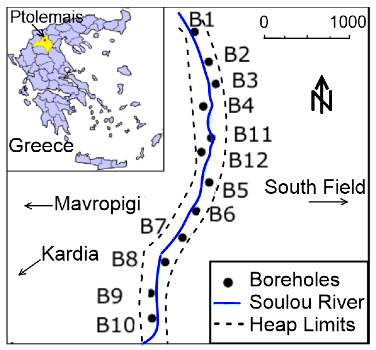
2.1. Study Area

Greece has been a major lignite producer and continues to play a significant role in the decarbonization period. During the period 2019–2022, 39.5 million metric tons of lignite were mined, primarily from deep surface mines, with the largest mining area being the Western Macedonia Lignite Centre. Within this mining complex, a massive spoil heap has accumulated, formed from materials excavated from adjacent lignite mines. The following information is a brief description of the study area and the experimental results that are used for the spatial variability analysis that follows and are based on previous works where they are more extensively described [3,25].

The typical ground profile in the mining area consists of a thick overburden zone mainly made of quaternary marls, clays, and some weak conglomerates and water-bearing sands overlying the lignite deposits. The spoil heap was initially constructed in 1999, with early using haul trucks, and later relying on continuous mining equipment, including belt conveyors and spreaders. The heap, measuring about 5 km in length, 150–170 m in height, and varying in width, has been a focal point of discussions regarding its long-term management and sustainable valorization.

Geotechnical investigations, including 12 boreholes drilled along the axis of the heap, provided the data on spoil materials (Figure 1). Laboratory tests assessed grain size distribution, Atterberg limits, and engineering parameters, revealing that fine-grained materials, mainly silts and clays, dominate the heap. The friction angle and cohesion were determined through 43 isotropically consolidated undrained triaxial tests with pore pressure measurements, while the constrained modulus and consolidation indices were measured in 61 oedometer tests. Despite some potential uncertainties in sample collection, the data present a comprehensive geotechnical overview of the spoil heap.

Some basic information regarding the spoil material types are presented; these information are based on [3] and are repeated here for the completeness of the present work. The classification of spoil materials according to the Unified Soil Classification System presents a great variety of different soil types that appear in a spatially random arrangement, ranging from coarse-grained gravels and sands to fine-grained silts and clays. However, an overview of the soil type classifications clearly indicates that the fine-grained materials are those which define the overall response of the spoil material. The major conclusion of [3] was that the spoil heap’s body is highly heterogeneous, while a significant outcome was the quantification of this variability, clearly indicating that spoil properties exceed the usual variability in in-situ ground materials. Due to this heterogeneity, but also other considerations extensively analyzed in that work, the spoil mass can be considered as one, unified spoil material with significant uncertainty.

While the earlier studies analyzed the statistical moments and cross-correlations of the spoil’s properties, this work goes further by examining the spatial variability in these properties, aiming to support more precise geotechnical analysis and design for future projects involving this complex material.

2.2. Quantification of Spoils’ Spatial Variability

Field and laboratory testing reveals considerable variability in soil properties, not only across the different sites and strata, but even within the deposits that appear homogeneous in a single location. This is unsurprising, since soils are usually formed by natural processes (e.g., weathering); transported to their present location; and subjected to various stress states, pore fluids conditions, and chemical transformations, resulting in significant spatial variability. Such spatial variability becomes even more pronounced in spoil heaps, where materials might originate from different mines being excavated with different methods, being transported with different methods, and in the end, being deposited with different methods, leading to notably high degrees of uncertainty, heterogeneity, and spatial variability. Although it is theoretically possible to characterize soil variability in great detail by conducting numerous tests, the sheer volume of testing required far exceeds the practical limits. Consequently, engineering practice typically relies on simplifications to account for this inherent variability.

Spatial characterization is typically introduced with the scale of fluctuation (SoF) [26,27]; below this distance, soils’ properties demonstrate a reasonably strong dependence. Small SoFs correspond to rapid fluctuations, while large ones show a strong correlation over long distances [28,29].

The SoF can be estimated using several methods; the autocorrelation function [26,27,28,29,30] and the semivariogram [31,32,33,34] are the most common. In this study, the semivariogram was adopted because it can be applied to non-uniformly spaced data (e.g., laboratory test data from various depths and distances).

The variogram function describes how much two observations depend on one another and how this dependence decreases as the distance increases. The semivariogram ($\gamma$)—half the variogram—is typically used and is defined as follows:

$$2\gamma =E\left\{{\left[z\left(x_i\right)-z\left(x_{i+h}\right)\right]}^2\right\}=Var[z\left(x_i\right)-z\left(x_{i+h}\right)]$$

(1)

where $\gamma$ is the semivariogram; E is the expected or mean value; Var is variance; $z\left(x_i\right)$ is the value of the examined property at location $x_i$; and h is the distance between the two locations under examination.

The principal characteristics of a semivariogram are the sill and the range. The sill is the ultimate variance where the empirical semivariogram appears to level off and theoretically equals data variance. The range is the distance at which the semivariogram reaches the sill. Several theoretical variogram models exist, such as the exponential, spherical, and Gaussian.

The following common steps were followed to obtain the semivariogram function. Initially, the so-called empirical semivariogram based on the experimental measurements was calculated using Equation (1) in all existing unique pairs of observations. The results were grouped in bins of the same size using [31] the following equation:

$$\gamma \left(h\right)={\displaystyle \frac{1}{2·N\left(h\right)}}·{\sum }_{i=1}^{N\left(h\right)}{{\left(z\right(x}_{i+h})-z(x_i\left)\right)}^2$$

(2)

where h is the distance between two observations ${z(x}_{i+h})$ and $z\left(x_i\right)$; and $N\left(h\right)$ is the total number of points existing in the particular bin. Each bin corresponds to a range of distances and is represented by the value resulting from Equation (2).

Furthermore, the exponential model was adopted, having two free parameters (sill and range) and being commonly used [35,36]:

$$\gamma \left(h\right)=C·(1-e^{\frac{-3h}{a}})$$

(3)

where $C$ is the sill and α is the range parameter. The SoF is directly related to the range parameter [37]:

$$\mathrm{S}\mathrm{o}\mathrm{F}={\displaystyle \frac{2}{3}}·\alpha$$

(4)

Finally, the exponential model was fitted onto the experimental data using the least-squares method. A supplementary approach, named in this work as the “conditional” exponential model, was employed in addition to the exponential model. The same exponential equation was used for that approach, but the sill of the model was assumed to equal data variance, which in this case is predetermined. Thus, the same equation (Equation (3)) was used for the conditional model, but it is a one-parameter equation having fixed the sill (C in Equation (3)).

Notice that the spatial variability in spoil properties depends highly on the direction. The effect of gravity and heap construction methods plays a definitive role. Consequently, the dataset for each property was analyzed, accounting for the vertical and the horizontal directions, eventually leading to two perpendicular scales. Significant differences of several orders of magnitude [37,38] have been observed between the horizontal and vertical SoFs for various materials. Notice that no values have been reported for spoils, as their spatial variability has not been quantified.

3. Spoil Spatial Variability

3.1. Overview

This section aims to characterize spatial variability targeting to quantify the scale of fluctuation (SoF). For each geotechnical parameter, two sets of analysis were performed in two perpendicular directions, vertical and horizontal. The two semivariograms and the associated scales of fluctuation were computed. The results provide insight into the spatial structure of the spoils and create a basis for further studies. All the properties have been examined and represent stationary variables; the various parameters have been checked with depth and for each borehole mainly visually, with a few cases when more data were available also being checked more systematically. Notice that spatial variability analysis is based on the data derived for a typical geotechnical analysis of the area, not conducted for this specific analysis (as typically is the case). Thus, there are limitations related to the distances between the boreholes, especially in the horizontal direction. The final results are an estimation of the scale of fluctuation and the order of magnitude of the range that should be included in stochastic analysis rather than an accurate calculation. They are also compared with the way the heap was created to reach useful conclusions on its peculiar structure.

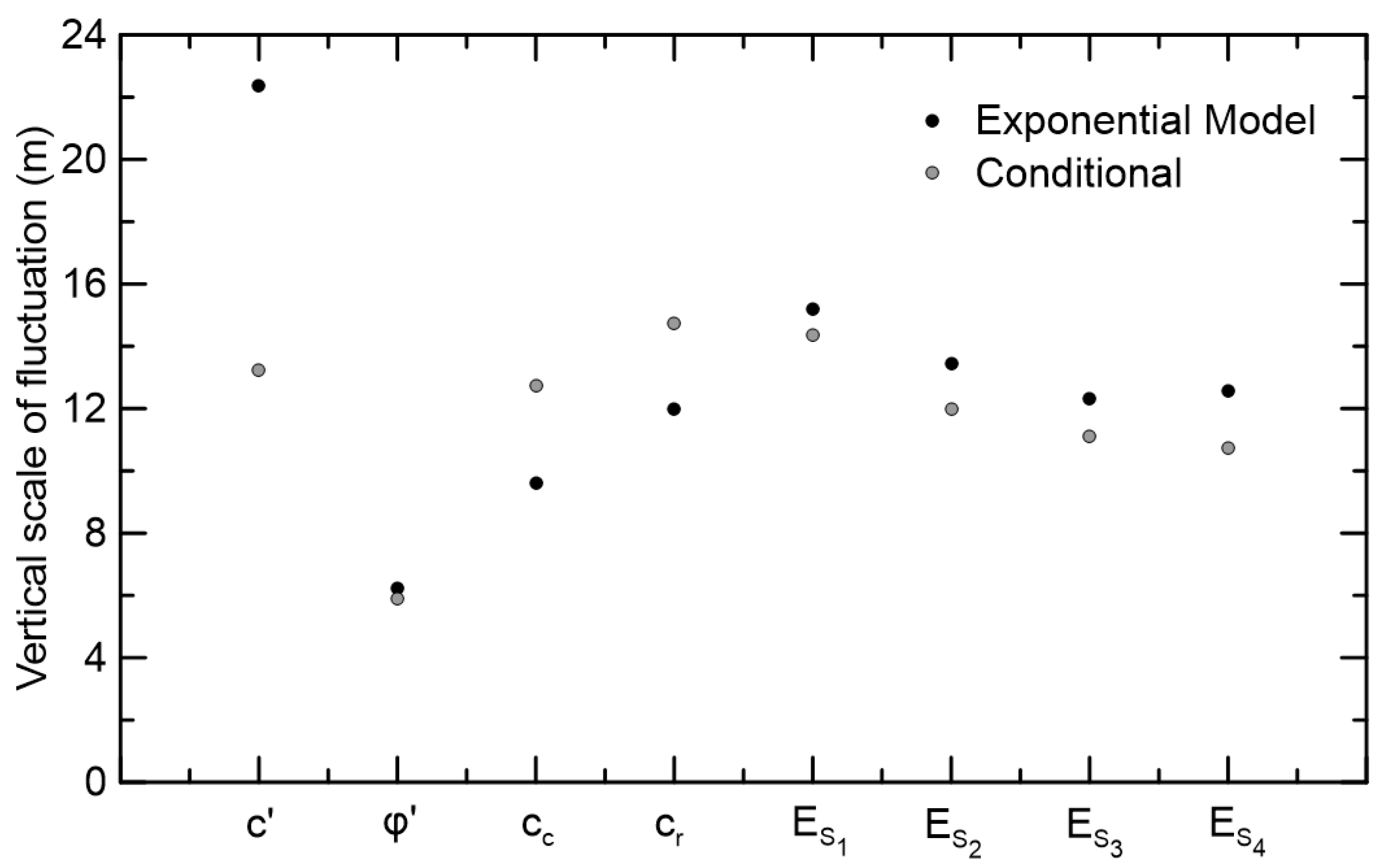
3.2. Vertical Scale of Fluctuation

Observations from a specific borehole were only paired with the others from the same borehole to ensure that only vertical correlations were involved in analysis. The pairs that emerged from all the twelve boreholes were then analyzed together, and an experimental semivariogram was created using Equation (2). Finally, one representative value for the vertical SoF was derived after fitting the theoretical model.

When creating the semivariogram, the rule of thumb is to consider at least half the maximum distance encountered [36]. Considering larger lag distances could lead to potential issues as model fitting would fit the longer distances when the shorter distances are the most important. In this analysis, the maximum depth was 50 m, and the maximum lag distance considered was 60%, i.e., 30 m. Most bins of the experimental variograms include a minimum of 30 pairs per bin [35]. Some bins include a minimum of 20–30 pairs and only a few less than 20. These few have been identified in this analysis and do not significantly alter the results.

Figure 2 and Figure 3 present all the semivariograms for the vertical direction, with the effective friction angle, cohesion, compression and recompression indices (Figure 2) and the constraint modulus for four different stress increments (Figure 3). The exponential model is presented with a black line. The conditional model approach is also presented; as mentioned in Section 2.2, the sill of the exponential model was assumed to be equal data variance, defining an equation identical to Equation (3) for the exponential model, but with one free parameter. Typically, this case (conditional fit) is not examined in the literature [28,39]; however, it evaluates the effect of the uncertainty of data variance. The comparison between the exponential and the conditional provides additional information regarding the accuracy of the resulting scale of fluctuation. Theoretically, the two approaches (exponential and conditional) are expected to provide identical results for large populations and lag distances. However, this is rarely the case in engineering practice, as less data than necessary are available. As a result, the difference between these two approaches is an indirect way to evaluate the appropriateness of the fit and obtain two estimations that define a range for the scale of fluctuation. Notice, however, that the difference between the two approaches is not a goodness-of-fit measure or a direct way to evaluate the variograms.

Regarding the appropriateness of the fit related to the small amount of data on small lags, notice that the curve fitting does not happen before the SoF, but before the range, which is exactly defined as the distance where the fitted curve first flattens out (becomes horizontal). The SoF characterizes the final fit, but does not determine the distance for the adequacy of the fit, which is best determined by the range. As a result, for example for Figure 2a, there are three points in the experimental variogram before the range and five points in Figure 2c.

Overall, the experimental semivariogram presents an increasing trend for small distances. Small lag distances are more significant since they define the line’s curvature, and thus the SoF. The semivariogram values located at large lag distances have a minor effect on fitting since the curve levels before it reaches them. In Figure 2a,c,d, the first ascending part of the curve follows the experimental values closely. The exponential or conditional fit lies above according to the relation between the sill value and statistical variance.

For effective friction angle, the two curves exhibit a very close identical initial part, yielding very close scales of fluctuation. This similarity of the two curves signifies that the population and the experimental variogram seem appropriate for the exponential model and the fitting procedure. For cohesion, the semivariogram presents larger variability compared to that of the friction angle, likely due to the many zero cohesion values in the dataset. The conditional fit diverges significantly from the exponential fit, indicating a high degree of uncertainty. The semivariograms of the compression and recompression indices exhibit a relatively smooth trend with a moderate sill, indicating consistent vertical correlation. The conditional model closely follows the exponential fit, meaning that the level of statistical uncertainty is significantly lower for this parameter compared to that for cohesion. The semivariogram fit is well aligned, reinforcing our confidence in the dataset’s reliability for these parameters.

Figure 3 illustrates the semivariograms of the constraint moduli. Overall, very similar trends are evaluated for all the stress increments. The conditional and exponential models propose a similar evolution. Additionally, the modulus increases with stress increments as expected, presenting stress-dependent spoil stiffness. Only the modulus for the highest stress increment (Figure 3d) presents greater variability, suggesting that at higher stress levels, heterogeneities in the spoil material’s stiffness might become more pronounced.

Figure 4 summarizes the SoFs for all the engineering parameters (the physical parameters LL and PI were omitted as they do not present similar interest regarding reliability analysis). The horizontal axis represents the examined parameters, while the vertical axis shows the vertical SoFs for the exponential model and its conditional version. For the constraint modulus E_s, the subscripts from one to four refer to the four corresponding stress increments of the experiment (50–100 kPa, 100–200 kPa, 200–400 kPa, and 400–800 kPa).

Figure 4 indicates that all the parameters exhibit comparable SoFs, except for effective cohesion. The results range from 5.9 m up to 16.2 m. The values of the exponential model and its conditional version are very close for all the parameters, except for effective cohesion; this signifies that the results for cohesion are not very reliable. This discrepancy can be due to cohesion’s large uncertainty that causes significant uncertainty in the quantification of the variogram. Overall, the compressibility parameters show similar values, but this is not the case for the effective strength parameters that present two different situations.

Effective cohesion is unique since many samples have zero values—a trend primarily due to the heterogeneous and loosely deposited nature of the spoil materials ([2,3,6,40]); the cohesion data present great uncertainty as also the statistical analysis indicates [25]. The resulting SoF is the largest among the tested parameters, and the difference between the exponential model and the conditional version is also the largest observed (41.1%). Note that the value for the conditional is very close to those of the other tested parameters. On the contrary, the effective friction angle presents the smallest SoF of all the parameters, and the SoF for the exponential model is very close to the one derived by the conditional version (difference of 4.8%).

The compressibility SoFs of the spoil are much more consistent. The compression and recompression indices have similar vertical scales of fluctuation. The compression index has the smallest SoF for the compressibility parameters, equal to 9.6 m; the recompression index exhibits a slightly higher value of 12 m. The conditional proposes higher SoFs than those of the exponential model for the compression and recompression indices by 24.4% and 23.2%, respectively.

Finally, the scales of fluctuation for the constraint modulus are also close, ranging from 10.8 m to 14.3 m. The conditional gives consistently smaller SoFs with relative differences ranging from 5.9% to 14.3%. The SoFs show a declining trend as the corresponding effective stress path increases, except for the 400–800 kPa stress path. This trend is much clearer for the conditional version of the model.

Overall, the vertical scales of fluctuation are within the literature range indicated by similar in-situ methods for natural soils [38], but among the highest values encountered. Their range denotes a medium degree of variability in the vertical direction. This relates to the construction method briefly discussed in Section 2.1; the boreholes are mainly from an area constructed with continuous methods (belts and spreaders), and thus vertical “zones” can propose similar properties when belonging to the same area of the same mine and have been transported in the same way. As a result, variability is presented when the mining area or the transportation way changes; thus, the scale of fluctuation is moderate.

3.3. Horizontal Scale of Fluctuation

Determining the horizontal SoF is more challenging due to the irregular spacing of the boreholes and the different heights at which the laboratory samples were obtained. However, this is the case for many geotechnical investigations. The data from a certain borehole were only paired with those of the other boreholes to exclude vertical correlation. However, the vectors created by the associated pairs of observations of the different boreholes are not purely horizontal since they are located at different depths. Instead, they form an angle with the horizontal plane; Figure 5 illustrates the distribution of these angles for the strength and compressibility parameters.

The differences between the two histogram parameters are negligible. Most pairs (more than 80%) form an angle of 0–2.5° with the horizontal plane, and approximately 99% form angles less than 10°. The remaining 1% of the pairs form angles reaching up to 25°. The limitations described and analyzed above could influence the final results, especially the large minimum horizontal distances for analysis. However, the results can still be considered indicative of this type of material and conditions. The same principles described previously for the vertical direction were applied to the semivariogram in the horizontal direction. The twelve boreholes lie on a polygonal chain of a total length approximately equal to 3.5 km. The maximum lag distance considered was therefore 2.0 km. The same three steps for creating the semivariogram were followed using the appropriate data pairs.

Figure 6 and Figure 7 illustrate all the properties as before for the semivariograms in the horizontal direction. Notice that the lag distances are two orders of magnitude higher than the vertical ones due to the distances between the boreholes. The horizontal range is significantly larger than the vertical one, indicating greater continuity in the horizontal direction. This suggests that frictional behavior is highly dependent on large-scale depositional patterns in spoil heaps. For the friction angle, the experimental values present an orderly ascending trend for the first few essential bins; the fit’s ascending part captures the initial experimental semivariogram trend quite well. However, after the curve reaches the sill, the deviations are significant.

This uncertainty may be due to sampling noise and limited data. Additionally, some paired values at these distances originate from significantly different geological conditions, resulting in unexpectedly high or low semivariance values. Beyond this, the observed variability may not be entirely random, but rather influenced by nested variability or secondary structures, where a larger-scale spatial pattern affects the data. These condition might be expected in a spoil material of this heterogeneity such as the one examined in this study. This uncertainty is a critical factor that can jeopardize future geotechnical projects on spoil heap sites. The risks arising from that uncertainty necessitate a detailed geotechnical investigation, incorporating advanced site characterization techniques, geostatistical modeling, and sensitivity analysis, to refine the understanding of spatial variability and mitigate uncertainties.

The appropriateness of the fit related to the small amount of data in the small lags, as also commented on earlier, was evaluated based on the range of the fitted model. Figure 6a shows three points in the experimental variogram before the range. However, for the experimental variogram shown in Figure 6c, fewer data are present at smaller lags (one point before the range), which means that the results for the compression (and recompression and constraint modulus) parameters on the horizontal SoF might not be as reliable as those for the other parameters.

Figure 8 illustrates the horizontal SoFs of the different engineering parameters. However, only the SoFs related to the strength parameters and not compressibility are reliable for this horizontal direction. Overall, the range of results is quite large, and the differences between the exponential model and its conditional version are larger than the vertical ones, indicating the higher uncertainties involved in the calculations.

The resulting SoF for effective cohesion is 161 m, the lowest value. The conditional version yields a lower value of 104 m. This difference is significant, but not the largest one observed. However, as mentioned previously, the data for effective cohesion were the most difficult to treat. Regarding the effective friction angle, the SoF is much larger, and the results for exponential and conditional are relatively close.

Overall, the scales of fluctuation in the horizontal direction are much higher than those in the vertical, as expected. The results of the exponential model and its conditional version generally present considerable differences. Finally, the results are within the range found in the literature, but above the average values [38].

Based on these SoFs, most geotechnical works that do not include linear infrastructure would not be drastically affected in the horizontal direction. The horizontal SoFs are large enough for surface-level and deep foundations (buildings, warehouses, and wind turbines) not to be considered in analysis. On the other hand, the various conditions in different areas should be considered for linear infrastructure, e.g., roads and railroads.

4. Discussion

The above analysis provides novel insights into the spatial variability in spoil materials, offering a perspective that has not been previously assessed. The accuracy of the SoF values lies on the reliability of the geotechnical data, including borehole logging; laboratory testing; and the interpretation of parameters, such as the friction angle, cohesion, and the compressibility indices. The data used in this analysis have been also systematically presented in [3] and are above the typical existing geotechnical data on spoil dumps.

The vertical SoF is influenced by borehole depth and sampling intervals, with boreholes drilled to a maximum depth of 50 m and test intervals varying based on the soil conditions. The relatively small vertical dataset introduces some bias in the semivariograms, particularly for the parameters with naturally high variability, such as cohesion. Additionally, the limited number of samples at greater depths reduces the confidence in SoF estimates for deeper layers, highlighting the need for more extensive vertical testing to improve reliability. Since only the borehole pairs from the same location were used for vertical analysis, short-range variability was well captured. This led to relatively small SoF values in the vertical direction (6.2–22.4 m), indicating localized changes in the soil properties.

For the horizontal SoF, the boreholes were spaced over a 3.5 km polygonal chain, resulting in large gaps in certain areas. The large horizontal distances (up to 2 km lag distance in the semivariograms) introduced high variability to the results. The horizontal SoFs were generally much larger than the vertical ones, reflecting the layered deposition nature of the spoil heap. However, the large distances between the boreholes meant that short-range horizontal variability might not be well represented. The semivariograms showed significant scatter at larger distances, particularly for the cohesion and modulus values, indicating that horizontal variability is not fully captured. The large horizontal SoFs (265–285 m) suggest that the properties are spatially continuous over long distances, which may be an overestimation due to data sparsity.

Finally, notice that this study relied on 12 boreholes distributed along the spoil heap. While sufficient for spatial analysis, denser borehole grids could enhance resolution, particularly for localized variations. Additionally, the boreholes were not evenly spaced in depth, leading to potential biases in semivariogram analysis. As many times in similar spatial analysis, this study assumes that spoil properties follow stationary random fields, but spoil heaps may exhibit non-stationary trends due to varying deposition processes.

5. Conclusions

The geotechnical characterization of spoil materials remains a challenge due to their inherent heterogeneity and complex depositional history. This study provided the spatial variability analysis of spoil materials within a lignite mine spoil heap, quantifying the scale of fluctuation (SoF) for key geotechnical parameters in both the vertical and horizontal directions. The findings contribute to a more robust understanding of spoil behavior, which is critical for stability analysis and future engineering applications.

The vertical SoF ranged from 6.2 m (friction angle) to 22.4 m (effective cohesion), indicating that the spoil properties change significantly over relatively short vertical distances. Effective cohesion is the most variable parameter, with a vertical SoF of 22.4 m, the highest of the tested parameters, and a horizontal SoF of 161 m, the lowest. The effective friction angle exhibited the opposite, with the vertical SoF at 6.2 m and the horizontal SoF reaching 265 m. For the compression and recompression indices, the vertical SoFs were 9.6 m and 12 m, respectively. The constraint modulus had comparable SoF values across the different stress increments (from 12.3 m to 15.2 m vertically).

In the horizontal plane, the dependence between the spoil elements is higher, with scales of fluctuation reaching 265 m for the friction angle and 285 m for the constraint modulus. Therefore, horizontally, the properties are almost uniformly distributed around the area of influence of most geotechnical applications, and a characteristic value of the property could be adopted.

The large horizontal SoFs indicate that geotechnical design parameters could be assumed constant over wide areas, benefiting linear infrastructure (e.g., roads and pipelines). The small vertical SoFs highlight the need for detailed investigations when designing foundations, slopes, and stability reinforcements. The findings of this study can inform the analysis and design of spoil heaps, with advanced numerical and stochastic tools providing a reliable approach for the geotechnical design of these highly heterogeneous materials.

Future research should focus on high-quality in-situ and laboratory data to enable robust statistical and spatial variability analyses. Dense grids of in-situ tests would facilitate such analysis, while a comprehensive database of spoil geotechnical properties and uncertainties is lacking. Finally, expanding semivariogram analysis to include 3D using geostatistical tools would better capture depositional patterns, while incorporating SoF values into numerical models would refine stability and settlement predictions.

References

1. International Energy Agency. Coal 2023—Analysis and Forecast to 2026. 2023. Available online: www.iea.org (accessed on 24 February 2025).
2. Masoudian, M.S.; Zevgolis, I.E.; Deliveris, A.V.; Marshall, A.M.; Heron, C.M.; Koukouzas, N.C. Stability and characterisation of spoil heaps in European surface lignite mines: A state-of-the-art review in light of new data. Environ. Earth Sci. 2019, 78, 505. [Google Scholar] [CrossRef]
3. Zevgolis, I.E.; Theocharis, A.I.; Deliveris, A.V.; Koukouzas, N.C.; Roumpos, C.; Marshall, A.M. Geotechnical Characterization of Fine-Grained Spoil Material from Surface Coal Mines. J. Geotech. Geoenviron. Eng. 2021, 147, 04021050. [Google Scholar] [CrossRef]
4. Kasmer, O.; Ulusay, R.; Gokceoglu, C. Spoil pile instabilities with reference to a strip coal mine in Turkey: Mechanisms and assessment of deformations. Environ. Geol. 2006, 49, 570–585. [Google Scholar] [CrossRef]
5. Vaníček, I.; Záleský, J.; Lamboj, L.; Kurka, J. Two examples of clay slope stability in areas affected by previous man-made activity—Open pit mines, landfills. In Proceedings of the 16th International Conference on Soil Mechanics and Geotechnical Engineering: Geotechnology in Harmony with the Global Environment, Osaka, Japan, 12–16 September 2005; pp. 2603–2606. [Google Scholar]
6. Zevgolis, I.E. Geotechnical characterization of mining rock waste dumps in central Evia, Greece. Environ. Earth Sci. 2018, 77, 566. [Google Scholar] [CrossRef]
7. Cadierno, J.F.; Romero, M.I.G.; Valdés, A.J.; del Pozo, J.M.M.; González, J.G.; Robles, D.R.; Espinosa, J.V. Characterization of Colliery Spoils in León: Potential Uses in Rural Infrastructures. Geotech. Geol. Eng. 2014, 32, 439–452. [Google Scholar] [CrossRef]
8. Ulusay, R.; Arikan, F.; Yoleri, M.; Çaǧlan, D. Engineering geological characterization of coal mine waste material and an evaluation in the context of back-analysis of spoil pile instabilities in a strip mine, SW Turkey. Eng. Geol. 1995, 40, 77–101. [Google Scholar] [CrossRef]
9. Wu, T.H.; Kraft, L.M. The Probability of Foundation Safety. J. Soil Mech. Found. Div. 1967, 93, 213–231. [Google Scholar] [CrossRef]
10. Ching, J.; Lee, S.-W.; Phoon, K.-K. Undrained strength for a 3D spatially variable clay column subjected to compression or shear. Probabilistic Eng. Mech. 2016, 45, 127–139. [Google Scholar] [CrossRef]
11. Wang, Y.; Zhao, T.; Cao, Z. Site-specific probability distribution of geotechnical properties. Comput. Geotech. 2015, 70, 159–168. [Google Scholar] [CrossRef]
12. Baecher, G.B.; Marr, W.A.; Lin, J.S.; Consla, J.A. Critical Parameters for Tailings Embankments; U.S. Department of the Interior: Denver, CO, USA, 1983.
13. Fenton, G.A.; Griffiths, D.V.; Zhang, X. Load and resistance factor design of shallow foundations against bearing failure. Can. Geotech. J. 2008, 45, 1556–1571. [Google Scholar] [CrossRef]
14. Griffiths, D.; Huang, J.; Fenton, G.A. Probabilistic infinite slope analysis. Comput. Geotech. 2011, 38, 577–584. [Google Scholar] [CrossRef]
15. Fenton, G.A.; Griffiths, D.V.; Williams, M.B. Reliability of traditional retaining wall design. Geotechnique 2005, 55, 55–62. [Google Scholar] [CrossRef]
16. Griffiths, D.V.; Fenton, G.A. Three-Dimensional Seepage through Spatially Random Soil. J. Geotech. Geoenviron. Eng. 1997, 123, 153–160. [Google Scholar] [CrossRef]
17. Ching, J.; Hu, Y.-G.; Phoon, K.-K. Effective Young’s modulus of a spatially variable soil mass under a footing. Struct. Saf. 2018, 73, 99–113. [Google Scholar] [CrossRef]
18. Firouzianbandpey, S.; Griffiths, D.; Ibsen, L.; Andersen, L. Spatial correlation length of normalized cone data in sand: Case study in the north of Denmark. Can. Geotech. J. 2014, 51, 844–857. [Google Scholar] [CrossRef]
19. Lloret-Cabot, M.; Fenton, G.; Hicks, M. On the estimation of scale of fluctuation in geostatistics. Georisk Assess. Manag. Risk Eng. Syst. Geohazards 2014, 8, 129–140. [Google Scholar] [CrossRef]
20. Bagińska, I.; Kawa, M.; Janecki, W. Estimation of spatial variability of lignite mine dumping ground soil properties using CPTu results. Stud. Geotech. Mech. 2016, 38, 3–13. [Google Scholar] [CrossRef]
21. Bagińska, I.; Kawa, M.; Janecki, W. Estimation of spatial variability properties of mine waste dump using CPTu results—Case study. In Cone Penetration Testing 2018; Hicks, M.A., Pisanò, F., Peuchen, J., Eds.; CRC Press: Delft, The Netherlands, 2018; pp. 109–115. [Google Scholar]
22. Olesiak, S. Influence of the heterogeneity of a dump soil on the assessment of its selected properties. Stud. Geotech. Mech. 2020, 42, 263–275. [Google Scholar] [CrossRef]
23. Thiruchittampalam, S.; Banerjee, B.P.; Glenn, N.F.; Raval, S. An Evaluation of Calibrated and Uncalibrated High-Resolution RGB Data in Time Series Analysis for Coal Spoil Characterisation: A Comparative Study. arXiv 2024, arXiv:2402.00170. Available online: https://arxiv.org/abs/2402.00170v1 (accessed on 5 March 2025).
24. Kumar, A.; Das, S.K.; Nainegali, L.; Reddy, K.R. Phytostabilization of coalmine overburden waste rock dump slopes: Current status, challenges, and perspectives. Bull. Eng. Geol. Environ. 2023, 82, 1–31. [Google Scholar] [CrossRef]
25. Theocharis, A.I.; Zevgolis, I.E.; Roumpos, C.; Koukouzas, N.C. Probability distributions of geotechnical properties for heterogeneous lignite mine spoils. Int. J. Geotech. Eng. 2024, 18, 528–536. [Google Scholar] [CrossRef]
26. Vanmarcke, E.H. Random Fields, Analysis and Synthesis; MIT Press: Cambridge, MA, USA, 1984. [Google Scholar]
27. Vanmarcke, E.H. Probabilistic Modeling of Soil Profiles. J. Geotech. Eng. Div. 1977, 103, 1227–1246. [Google Scholar] [CrossRef]
28. Bong, T.; Stuedlein, A.W. Spatial Variability of CPT Parameters and Silty Fines in Liquefiable Beach Sands. J. Geotech. Geoenviron. Eng. 2017, 143, 04017093. [Google Scholar] [CrossRef]
29. Stuedlein, A.W.; Kramer, S.L.; Arduino, P.; Holtz, R.D. Geotechnical Characterization and Random Field Modeling of Desiccated Clay. J. Geotech. Geoenviron. Eng. 2012, 138, 1301–1313. [Google Scholar] [CrossRef]
30. Baecher, G.B.; Christian, J.T. Reliability and Statistics in Geotechnical Engineering; John Wiley & Sons: West Sussex, UK, 2003. [Google Scholar]
31. Matheron, G. Principles of geostatistics. Econ. Geol. 1963, 58, 1246–1266. [Google Scholar] [CrossRef]
32. Malvić, T.; Ivšinović, J.; Velić, J.; Rajić, R. Kriging with a Small Number of Data Points Supported by Jack-Knifing, a Case Study in the Sava Depression (Northern Croatia). Geosciences 2019, 9, 36. [Google Scholar] [CrossRef]
33. Caballero, S.R.; Bheemasetti, T.V.; Puppala, A.J.; Chakraborty, S. Geotechnical Visualization and Three-Dimensional Geostatistics Modeling of Highly Variable Soils of a Hydraulic Fill Dam. J. Geotech. Geoenviron. Eng. 2022, 148, 05022006. [Google Scholar] [CrossRef]
34. Sitharam, T.G.; Samui, P. Geostatistical modelling of spatial and depth variability of SPT data for Bangalore. Géoméch. Geoeng. 2007, 2, 307–316. [Google Scholar] [CrossRef]
35. Cressie, N.A.C. Statistics for Spatial Data Revised Edition; Wiley: Hoboken, NJ, USA, 2015. [Google Scholar] [CrossRef]
36. Journel, A.G.; Huijbregts, C.J. Mining Geo-Statistics; Academic Press: London, UK, 1978. [Google Scholar]
37. Technical Committee of Engineering Practice of Risk Assessment & Management (TC304 ISSMGE). State-of-the-Art Review of Inherent Variability and Uncertainty in Geotechnical Properties and Models; ISSMGE. 2021. Available online: https://issmge.org/files/reports/TC304-State-of-the-art-review-of-inherent-variability-and-uncertainty-in-geotechnical-properties-and-models.pdf (accessed on 5 March 2025). [CrossRef]
38. Cami, B.; Javankhoshdel, S.; Phoon, K.-K.; Ching, J. Scale of Fluctuation for Spatially Varying Soils: Estimation Methods and Values. ASCE-ASME J. Risk Uncertain. Eng. Syst. Part A Civ. Eng. 2020, 6, 03120002. [Google Scholar] [CrossRef]
39. Onyejekwe, S.; Ge, L. Scale of Fluctuation of Geotechnical Parameters Estimated from CPTu and Laboratory Test Data. In Foundation Engineering in the Face of Uncertainty; American Society of Civil Engineers: Reston, VA, USA, 2013; pp. 434–443. [Google Scholar] [CrossRef]
40. Garala, T.K.; Cui, G.; Kantesaria, N.; Heron, C.M.; Marshall, A.M.; Žižka, L. Characterisation of spoil materials to develop an equivalent spoil material for physical model tests. Górnictwo Odkrywkowe (Surf. Min.) 2022, 4, 23–29. [Google Scholar] [CrossRef]
Figure 1. The location of the spoil heap in Greece and a map of the borehole locations.
Geosciences 15 00097 g001
Figure 2. The semivariogram for the vertical direction of (a) the effective friction angle φ’ and (b) effective cohesion (c) the compression index cc, and (d) the recompression index cr.
Geosciences 15 00097 g002
Figure 3. The semivariogram for the vertical direction of the constraint modulus for (a) Δσ’ = 50 kPa, (b) Δσ’ = 100 kPa, (c) Δσ’ = 200 kPa, and (d) Δσ’ = 400 kPa.
Geosciences 15 00097 g003
Figure 4. Vertical scale of fluctuation for geotechnical parameters. c’: cohesion; φ’: friction angle; cc: compression index; cr: recompression index; Es1: constraint modulus (Δσv = 50 kPa); Es2: constraint modulus (Δσv = 100 kPa); Es3: constraint modulus (Δσv = 200 kPa); Es4: constraint modulus (Δσv = 400 kPa).
Geosciences 15 00097 g004
Figure 5. The angles formed between the vector created from pairs of observations and the horizontal plane for (a) the effective strength and (b) the compressibility spoil parameters.
Geosciences 15 00097 g005
Figure 6. The semivariogram for the horizontal direction of (a) the effective friction angle φ’, (b) effective cohesion, (c) the compression index cc, and (d) the recompression index cr.
Geosciences 15 00097 g006
Figure 7. The semivariogram for the horizontal direction of the constraint modulus for (a) Δσ’ = 50 kPa, (b) Δσ’ = 100 kPa, (c) Δσ’ = 200 kPa, and (d) Δσ’ = 400 kPa.
Geosciences 15 00097 g007
Figure 8. Horizontal scale of fluctuation for geotechnical parameters. c’: cohesion; φ’: friction angle; cc: compression index; cr: recompression index; Es1: constraint modulus (Δσv = 50 kPa); Es2: constraint modulus (Δσv = 100 kPa); Es3: constraint modulus (Δσv = 200 kPa); Es4: constraint modulus (Δσv = 400 kPa).
Geosciences 15 00097 g008
Disclaimer/Publisher’s Note: The statements, opinions and data contained in all publications are solely those of the individual author(s) and contributor(s) and not of MDPI and/or the editor(s). MDPI and/or the editor(s) disclaim responsibility for any injury to people or property resulting from any ideas, methods, instructions or products referred to in the content.