Scaling Law Analysis and Aftershock Spatiotemporal Evolution of the Three Strongest Earthquakes in the Ionian Sea During the Period 2014–2019

Abstract

The observed scaling properties in the three aftershock sequences of the recent strong earthquakes of magnitudes M_w 6.1, M_w 6.4 and M_w 6.7, which occurred in the Ionian island region on the 26 January 2014 (onshore Cephalonia Island), 17 November 2015 (Lefkada Island) and 25 October 2018 (offshore Zakynthos Island), respectively, are presented. In the analysis, the frequency–magnitude distributions in terms of the Gutenberg–Richter scaling relationship are studied, along with the temporal evolution of the aftershock sequences, as described by the Omori–Utsu formula. The processing of interevent times distribution, based on non-extensive statistical physics, indicates a system in an anomalous equilibrium with long-range interactions and a cross over behavior from anomalous to normal statistical mechanics for greater interevent times. A discussion of this cross over behavior is given for all aftershock sequences in terms of superstatistics. Moreover, the common value of the Tsallis entropic parameter that was obtained suggests that aftershock sequences are systems with very low degrees of freedom. Finally, a scaling of the migration of the aftershock zones as a function of the logarithm of time is discussed regarding the rate strengthening rheology that governs the evolution of the afterslip process. Our results contribute to the understanding of the spatiotemporal evolution of aftershocks using a first principles approach based on non extensive statistical physics suggesting that this view could describe the process within a universal view.

1. Introduction

The Ionian Islands are a very seismically active region in Greece. On the 26 January 2014 (13:55:42 UTC) and 3 February 2014 (03:08:45 UTC), two strong earthquakes of M_w 6.1 and M_w 6.0, respectively, occurred onshore of the island of Cephalonia [1]. These seismic events caused considerable structural damage and environmental effects, particularly in the western and central regions of the island [2]. On 17 November 2015 (07:10:07 UTC) another strong event that reached a magnitude of M_w 6.4 hit, this time on Lefkada Island. In addition, a quite strong earthquake of M_w 6.7 occurred on 25 October 2018 (22:54:51 UTC) offshore of Zakynthos Island, but with only moderate damage reported [3,4]. In contemporary times, this area has experienced major and destructive earthquakes, such as those that ruptured the eastern part of Cephalonia Island on 9, 11 and 12 August 1953, with surface-wave magnitudes of 6.4, 6.8 and 7.2, respectively [5]. Additionally, on 17 January 1983, a powerful (Mw7.0) earthquake ruptured the western offshore area, resulting in no significant damage [6,7]. Seismic excitations in this area are the result of right-lateral shear strain accumulated in a zone of weakness, which abuts and slightly overlaps the rupture area of the 1983 main shock (M_w 7.0) [8,9].

In this paper, we examine the temporal evolution and scaling properties of the aftershock sequences that followed the three recent major earthquakes that struck the Ionian Islands between 2014 and 2019. First, we calculate the scaling parameters of well-established empirical scaling relationships for aftershock sequences, such as the Omori–Utsu formula [10] for the aftershocks decay rate and the Gutenberg–Richter scaling relationship [11] for the frequency–magnitude distribution of seismicity.

In addition, in recent years, strong evidence indicates that the earthquake generation process can be analyzed in terms of the Complexity theory [12,13,14,15,16]. The characterization of time dynamics associated with an earthquake sequence provides strong evidence for the presence of an underlying spatiotemporal nonlinear deterministic dynamical process [17,18,19]. The time–space behavior that was observed can be mapped by fractal (self-similar) properties including power law distributions, spatiotemporal clustering and long-range correlations [17,20] and can describe the earthquake’s spatial and temporal distribution [21,22,23]. Such properties, along with a broad range of geodynamic phenomena connected to complexity dynamics, display intriguing characteristics when viewed within novel frameworks, such as those of non-extensive statistical physics [24].

This work is motivated by the historical occurrences of major earthquakes along the Cephalonia Transform Fault and the broader Ionian Island region [5], along with the need to extend our knowledge regarding seismic hazards in the area using modern and innovative methodologies. The present work seeks to explore the scaling properties and the applicability of the complexity theory and Non-Extensive Statistical Physics (NESP) in the aftershock sequences of the three recent strong earthquakes in the Ionian Islands. Our results contribute to the understanding of the spatiotemporal evolution of aftershocks using a first principles approach based on non-extensive statistical physics suggesting that this view could describe the process within a universal view.

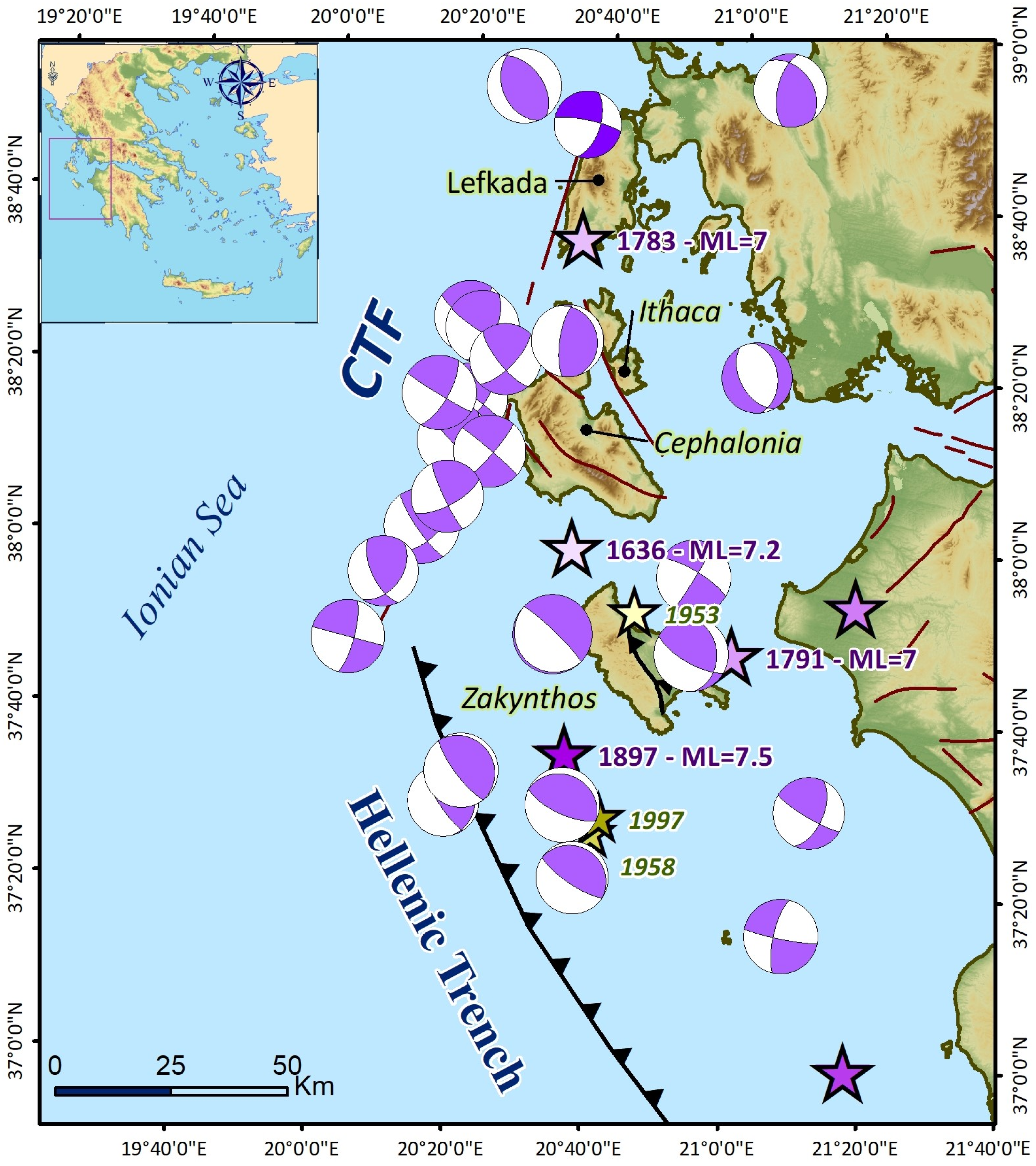
2. Seismotectonic Regime of Cephalonia, Lefkada and Zakynthos Islands

The Ionian Islands, located in Western Greece, are situated in a seismotectonically intricate region characterized by rapid and significant ground deformation. Cephalonia Island, positioned centrally within the Ionian area (Figure 1), accommodates a remarkable seismic history [5]. The island’s formation occurred during the Tertiary period as a result of the convergence between the African and the Eurasian tectonic plates that initiated at the end of the Cretaceous ([25] and references therein).

The island of Cephalonia has been repeatedly subjected to strong ground shaking due to the proximity of the Cephalonia Transform Fault (CTF) (see Figure 1). The CTF is situated offshore to the west of Cephalonia Island and is a major strike-slip fault that connects the subduction boundary in the south to the continental collision between the Apulian microplate and the Hellenic foreland in the north [26,27], playing a significant role in the region’s geodynamic complexity [28] (Figure 1). Its slip-rate ranges from 7 to 30 mm/yr [29], which is consistent with seismological data [30,31].

For the study area, comprehensive historical data for strong seismic events of magnitude M ≥ 6.5 exist during the last five centuries, indicating an average occurrence of approximately one such event per decade [32]. The most severe was the 1953 paroxysm with four events (9 August, M 6.4; 11 August, M 6.8; 12 August, M 7.2; 21 October, M 6.3) that almost destroyed completely the infrastructures on the Cephalonia Island. Other recent strong CTF events include the M 6.8 on 17 January 1983, and the M 6.2 on 14 August 2003. Additionally, the earliest known historical event of magnitude M 7.0 occurred in 1469 AD, which caused extensive damage on the Cephalonia Island, as well as the M 6.3 and M 7.4 earthquakes which took place close to Lixouri town, on 22 July 1767, and 4 February 1867, respectively [32]. Three strong earthquakes occurred in 1915 close to Ithaca Island, while other destructive events include the magnitudes Mw 6.9, Mw 6.3 and Mw 6.8 on 12 August 1953, 21 October 1953 and 15 November 1959, respectively, as well as four major events with magnitudes Mw 6.2, Mw 6.8, Mw 6.1 and Mw 6.5 on 17 September 1972, 17 January 1983, 23 March 1983 and 18 November 1997, respectively (Figure 1) [26,31].

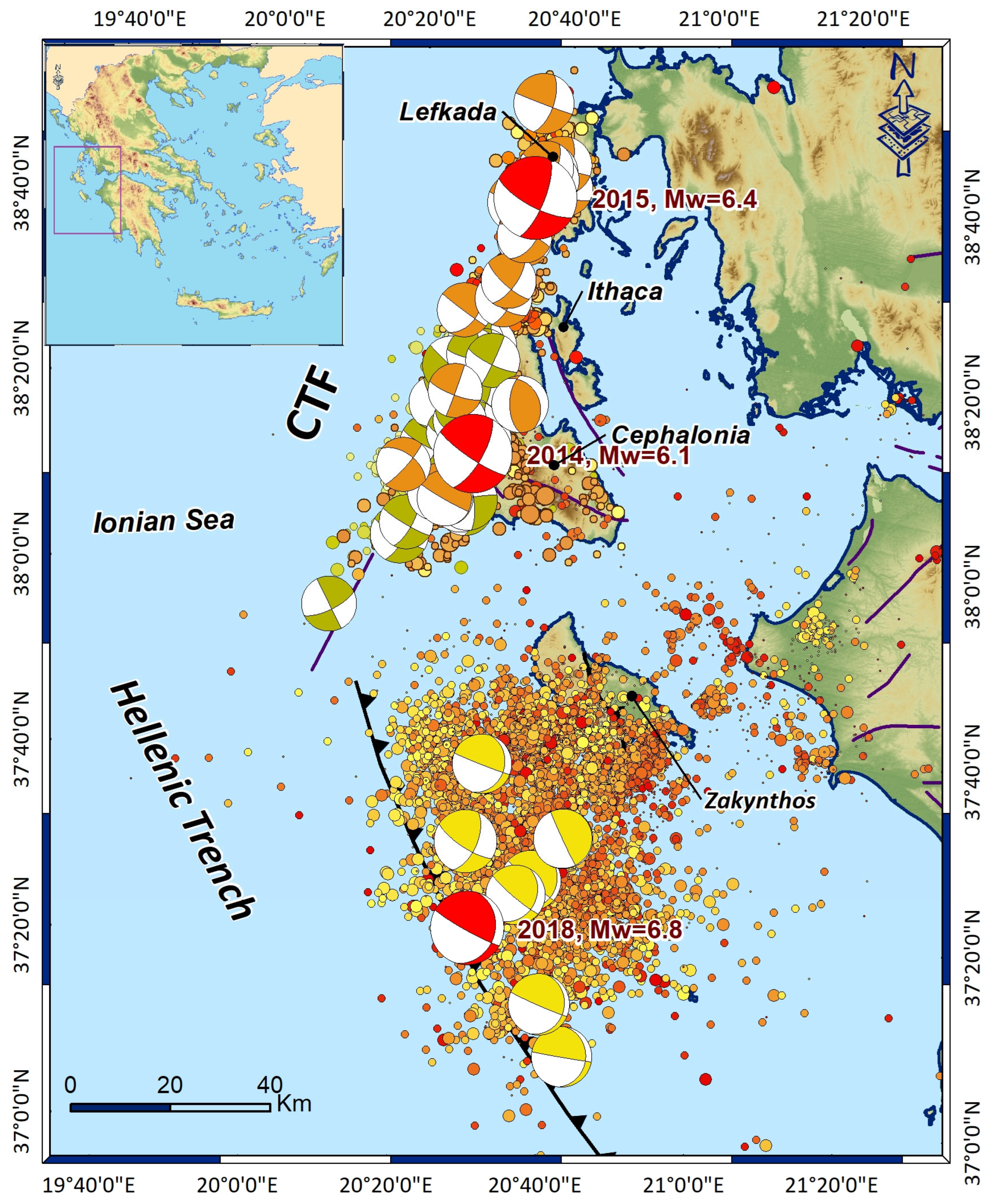
3. Seismological Data

The seismological data used for the period 2014–2019 were obtained from the open-access database of the seismological laboratory of the National and Kapodistrian University of Athens (http://dggsl.geol.uoa.gr/en_index.html, accessed on 18 February 2025) (Figure 2). The events selected are shallow ones with a focal depth of less than 30 km and the aftershock sequences defined combining a visual inspection with the results presented in [33].

The area of study is covered by several local stations belonging to the Hellenic Unified Seismological Network (HUSN) [34]. All the event locations used in the catalogue were calculated using manually picked P- and S-wave arrival times, the HYPOINVERSE algorithm [35], and a regional 1-D velocity model consisting of eight layers as described in [36].

The root mean square residual (RMS) for the initial aftershock sequence following the 2014 Cephalonia Mw 6.1 earthquake was determined as 0.24, while the mean of the horizontal and vertical directions uncertainties for the events hypocenters are 0.51 km and 1.08 km, respectively. For the second and third aftershock sequences, associated with the 2015 Lefkada Mw 6.4 and the 2018 Zakynthos Mw 6.8 earthquakes, RMS was calculated as 0.8 and 0.32, respectively, while the mean of the horizontal directions uncertainties are 1.97 km and 2.06 km and for the vertical 4.37 km and 2.1 km, respectively. In addition, fault plane solutions for the Cephalonia, Lefkada and Zakynthos mainshocks are in Figure 2.

The earthquake epicenters in the Cephalonia region show slightly better results than those in Lefkas regarding spatial and temporal errors (RMS, ERH and ERZ). This may be attributed initially to the coverage of the available events, especially for those located on the Paliki peninsula and in the Gulf of Myrtos, with HUSN stations, compared to the corresponding earthquakes in Lefkas Island, where the majority of the dataset is located in the offshore area, which has the largest azimuthal gap in the available catalogue.

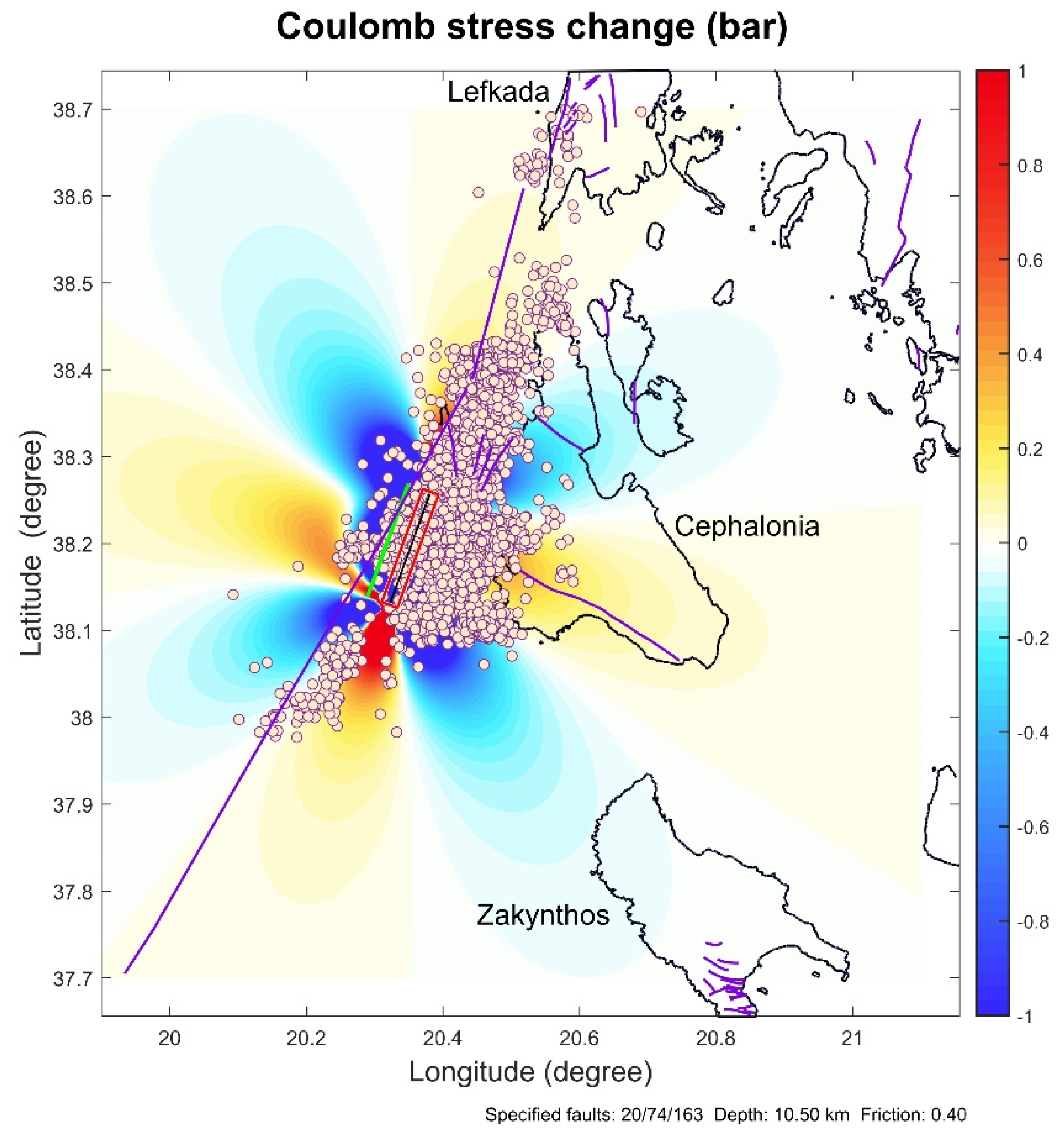
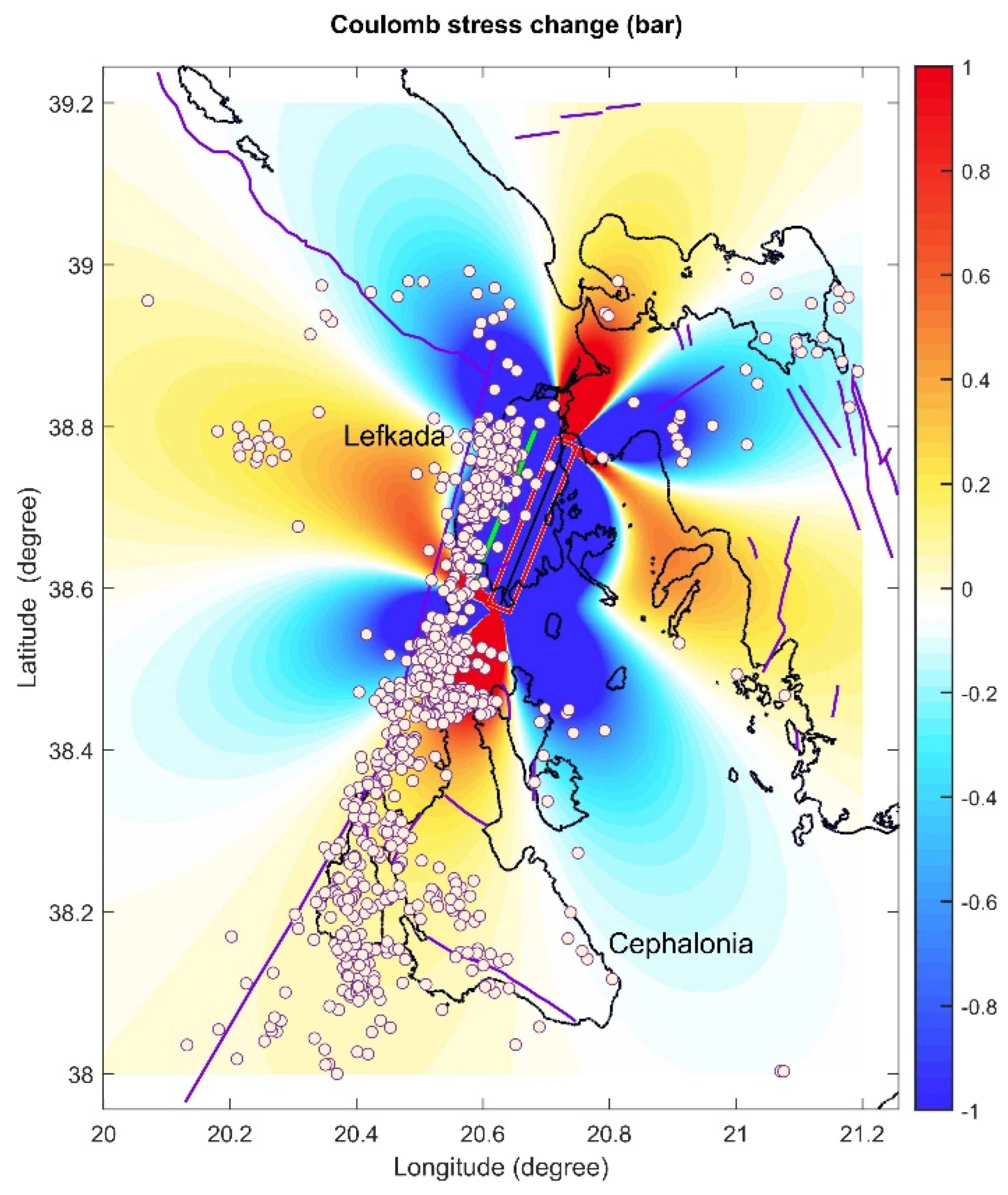
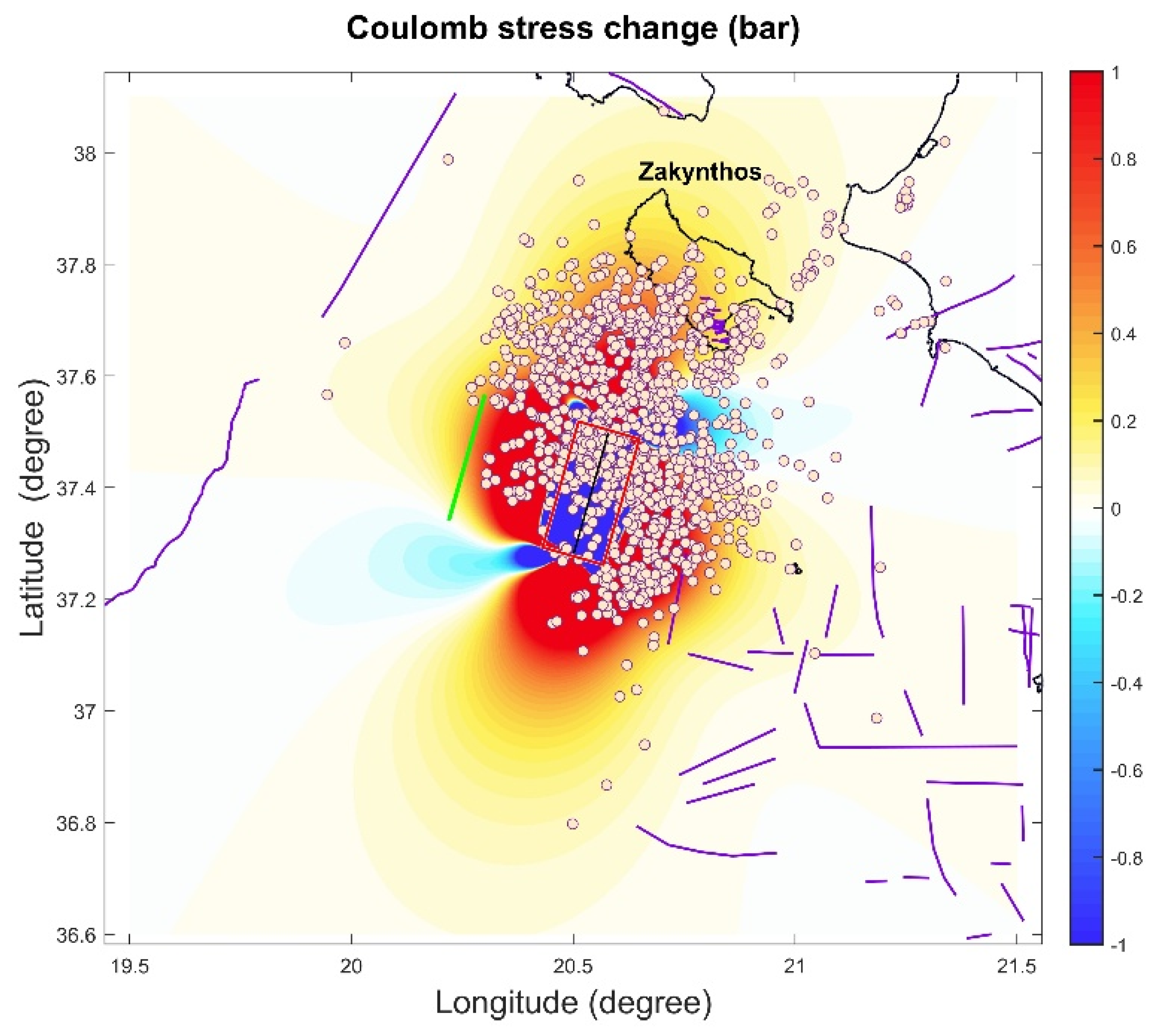
4. Coulomb Stress Changes of the Three Major Ionian Islands Events

Many seismologists have focused on Coulomb Stress changes and how static Coulomb Stress transfer to nearby faults that meet critical conditions might cause subsequent earthquakes [37,38,39,40,41]. The triggering of subsequent aftershocks due to static coulomb stress transfer to neighboring faults which fulfill critical conditions.

The stress evolution depends on tectonic movements as well as the orientation of coulomb stress transfer due to fault activation. The static stress changes generated during rupture due to a significant earthquake can govern the aftershock spatial and temporal distribution [3,42,43,44]. Strong earthquakes have been shown to cause Coulomb failure stress changes (ΔCFS), which can influence and extend the temporal and spatial distribution of a seismic sequence evolution and accelerate or slow down future earthquakes [41,45,46].

The calculation of Coulomb Failure Stress changes (ΔCFS) relies on the Coulomb failure criterion, which defines the conditions under which the failure occurs in rocks. According to this approach, we determined the spatial distribution of the Coulomb stress changes for the three mainshocks. For this purpose, we used the software Coulomb 3.3 to simulate the Coulomb Failure Stress changes (ΔCFS) using the parameters of Centroid moment tensor (CMT) focal mechanisms, (

Table 1. Focal mechanisms CMT of the three significant earthquakes (see text for details).

Date Time	Lat	Lon	Depth (km)	Mw	Strike	Dip	Rake	Seismic Moment (in Nm)
26 January 2014 13:55 [47]	38.1944	20.3519	10.5	6.1	20	74	163	1.40 × 1018
17 November 2015 07:10 [48]	38.6785	20.5889	14	6.4	22	72	161	4.30 × 1018
25 October 2018 22:54 [4]	37.3939	20.5400	12	6.7	16	25	166	9.05 × 1018

) and a coefficient of friction of 0.4 [4,47,48] (www.geol.uoa.gr).

The calculation of Coulomb Stress changes (ΔCFS) is founded on the Coulomb failure criterion which describes the conditions of rock rupture and is defined as follows

ΔCFS = Δτ + μ_f (Δσ + Δp)

(1)

where Δp is the change in pore pressure inside the fault plane, μf is the friction coefficient, which, in dry conditions, varies from 0.6 to 0.8, and Δτ and Δσ are the shear and normal stress changes, respectively (ref. [49] and references therein). We consider the undrained conditions [50], in which the fluid mass per unit volume is assumed to be constant and Δp is dependent on the fault–normal stress. Furthermore, we disregard variations in pore fluid pressure that occur throughout time. Rice and Cleary’s [51] method of calculating induced changes in pore pressure resulting from a change in stress under undrained conditions is Δp = −B (Δσ_kk/3) where B is Skempton’s coefficient (0 < B < 1), and Δσkk the summation over the diagonal elements of the stress tensor. For granites, sandstones, and marbles, experimental estimates of B range from 0.5 to 0.9 [51]. The calculation of Δσkk and Δτ is founded on the fault plane solution of the target fault, whose triggering is examined. The shear modulus and Poisson’s ratio were fixed at 3.3 MPa and 0.25, respectively [52,53].

The Coulomb stress changes (ΔCFS) of the Cephalonia Mw 6.1 earthquake revealed a transfer of positive values towards the Lefkada Island (Figure 3), while the ΔCFS results of the Mw 6.4 Lefkada earthquake revealed a transfer of positive values towards the Cephalonia Island (Figure 4). The latter justifies the possible triggered seismic activity in Cephalonia during 2016 due to the Mw 6.4 Lefkada earthquake. The ΔCFS positive values of the Mw 6.7 Zakynthos earthquake follow the same direction as the previous two major events (Figure 5).

5. Scaling Properties in Aftershock Sequences: Methods Used

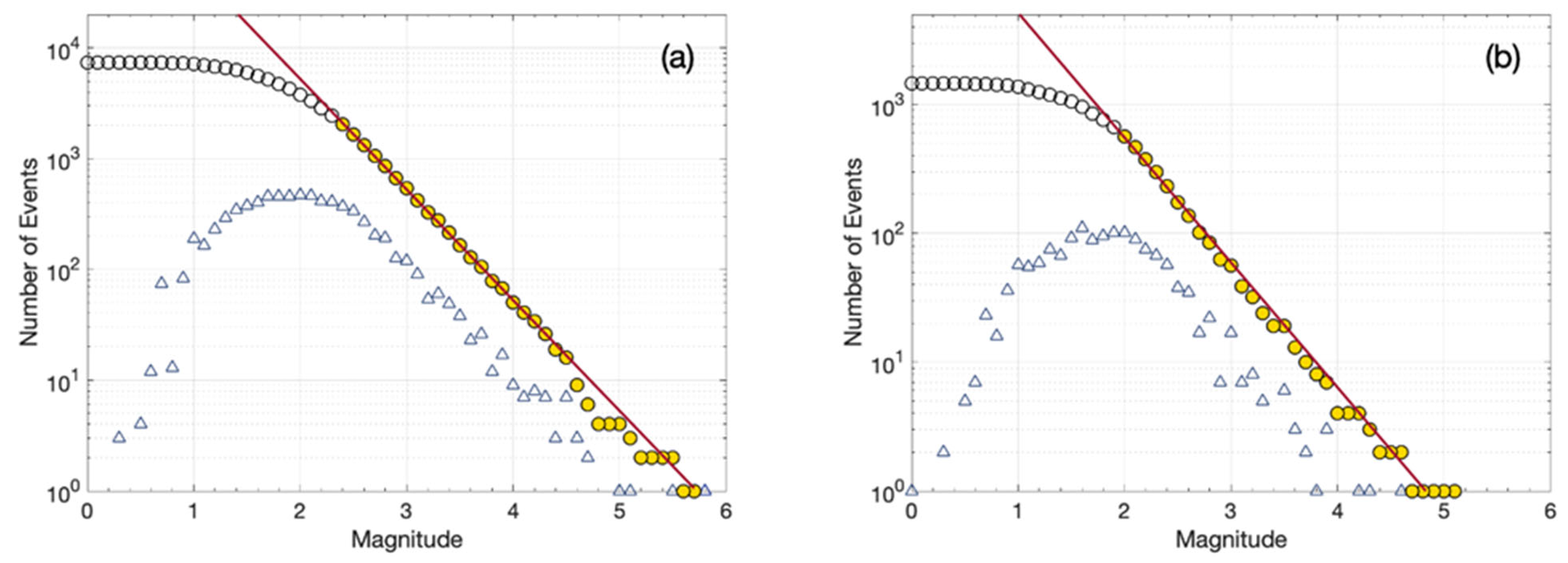
5.1. The Frequency–Magnitude Distribution

For each aftershock sequence we could estimate the frequency–magnitude distribution (FMD) as the cumulative number of events N(>Mw) with a magnitude greater than Mw. The FMD typically scales according to the Gutenberg–Richter (G–R) scaling relationship above some given threshold magnitude, which is frequently considered as the magnitude of completeness (Mc) of the seismic catalog. The G–R relationship is given as [54],

logN (>M_w) = a − b M_w

(2)

where a and b stand for positive constants that, respectively, indicate the ratio of smaller to greater magnitude events and the amount of regional seismicity. The seismic b-value, also known as the parameter b, typically takes values near to one [55,56]. This pattern is also seen in aftershock sequences (e.g., [57,58,59,60]).

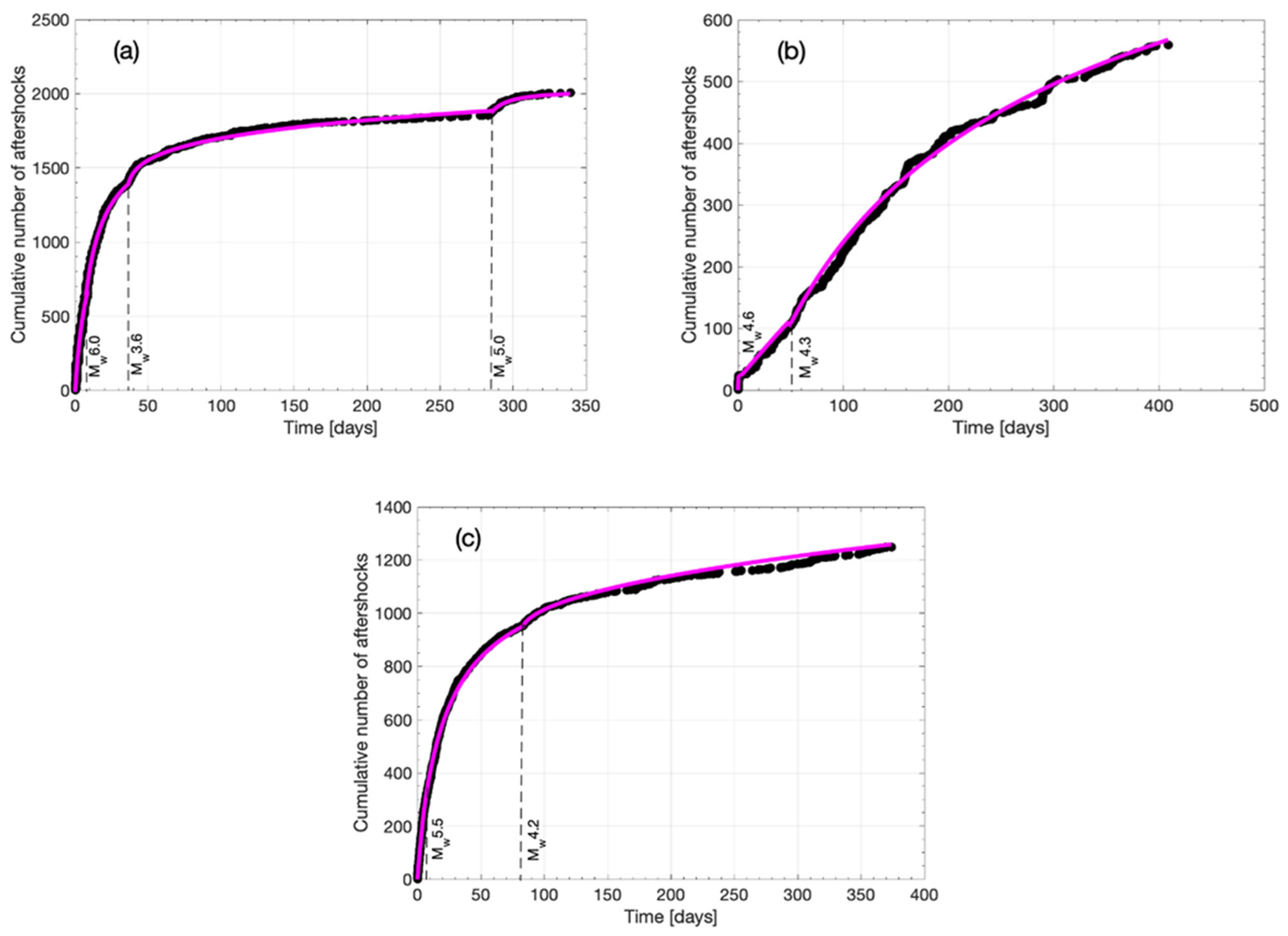
5.2. Temporal Scaling Properties

The temporal scaling properties of aftershock sequences are typically studied in terms of the aftershocks production rate $n\left(t\right)=dN\left(t\right)/dt$, where N(t) is the number of aftershocks in time t following the mainshock. The aftershocks production rate n(t) typically scales as an inverse power-law with time t according to the modified Omori formula [61,62]:

$$n\left(t\right)=K{\left(t+c\right)}^{-p}$$

(3)

where p is the power-law exponent that typically takes values close to one, K a proportionality constant that expresses the total number of aftershocks and c a characteristic positive constant [61]. In terms of the cumulative number of aftershocks N(t), the modified Omori formula is expressed as:

$$N\left(t\right)=\left\{\begin{array}{c}K\left[c^{1-p}-{\left(t+c\right)}^{1-p}\right]/\left(p-1\right),forp\ne 1\\ Kln\left(t/c+1\right),forp=1\end{array}\right.$$

(4)

In addition, strong aftershocks can trigger their own aftershock sequences, signifying several modified Omori regimes embedded within the mainshock’s aftershock sequence. In this case, the aftershock production rate n(t) can be expressed as [61,63]:

$$\mathit{n}\left(\mathit{t}\right)={\mathit{K}}_1{\left(\mathit{t}+{\mathit{c}}_1\right)}^{-{\mathit{p}}_1}+\mathit{H}\left(\mathit{t}-{\mathit{t}}_2\right){\mathit{K}}_2{\left(\mathit{t}-{\mathit{t}}_2+{\mathit{c}}_2\right)}^{-{\mathit{p}}_2}+\mathit{H}\left(\mathit{t}-{\mathit{t}}_3\right){\mathit{K}}_3{\left(\mathit{t}-{\mathit{t}}_3+{\mathit{c}}_3\right)}^{-{\mathit{p}}_3}$$

(5)

In the previous equation, t₂, t_3, etc. mark the occurrence time of strong aftershocks, while H(·) represents a unit step function.

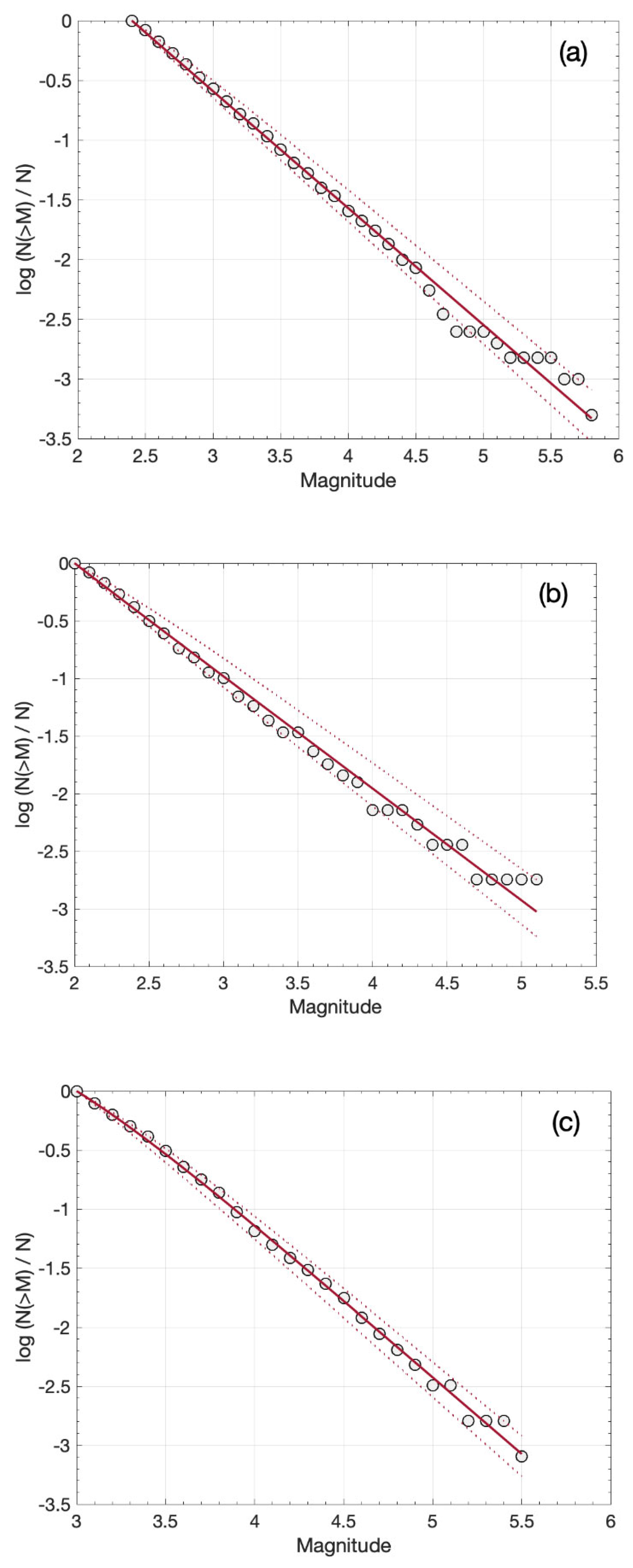
5.3. Earthquake Scaling Properties in Terms of Non-Extensive Statistical Physics

The aftershock sequences could be explored in terms of non-extensive statistical physics (NESP), a theoretical framework originally proposed by Tsallis [24,64]. The NESP offers the advantage of effectively illustrating the spatiotemporal dynamics of seismic activity through the universal principle of entropy. The foundation of NESP builds upon a generalization of Boltzmann–Gibbs (BG) statistical physics, enabling the analysis of systems characterized by long-range interactions and long-term memory. The expression of the non-additive Tsallis entropy S_q [65] in terms of a fundamental parameter’s X probability distribution p(X), is:

$$S_q=k_B{\displaystyle \frac{1-\sum p^q\left(X\right)}{q-1}}$$

(6)

where $k_B$ is the Boltzmann constant while the q is the so-called entropic index which is the degree of non-additivity. In the particular case where q = 1, then, $S_q=S_{BG}$ and the BG entropy is obtained.

Despite the fact that $S_q$ and $S_{BG}$ have many common characteristics, including concavity, expansibility, and non-negativity, they differ in terms of additivity. While the Tsallis entropy $S_q$ (with q ≠ 1) is non-additive, the BG entropy is additive, which means that the entropy of a coupled system is equal to the sum of the entropies of its constituent components. For any two probabilistically independent systems, A and B, the Tsallis entropy follows the following expression:

$$S_q\left(A+B\right)=S_q\left(A\right)+S_q\left(B\right)+{\displaystyle \frac{\left(q-1\right)}{k_B}}{S}_q(A)S_q(B)$$

(7)

This basic principle governs non-extensive statistical physics. Specifically, q < 1 indicates superadditivity, q > 1 indicates subadditivity, and finally, Equation (7)’s right-hand side vanishes when q = 1, indicating the additivity feature as predicted by conventional BG statistics.

As was previously indicated, Tsallis [24] proposed NESP as a generalization of BG statistical physics, providing a logical theoretical framework for the analysis of complex dynamical systems with long-range correlations and fractal properties [24]. In order to determine the earthquake frequency–magnitude distribution function, Silva et al. [66] revised the fragment–asperity model. The model [66] assumes that the eventual relative position of fragments filling the space between two irregular faults can hinder their relative motion. Stress increases until the displacement of one of the asperities, due to the displacement of the hindering fragment, or even its breakage in the point of contact with the fragment leads to a relative displacement of the fault planes of the order of the size of the hindering fragment, with the subsequent energy release. Taking into account Telesca’s [67] expression between magnitude and released relative energy, $M~{\displaystyle \frac{2}{3}}\log \left(E\right)$, the cumulative distribution in terms of earthquake magnitude can be calculated.

In order to account for the threshold magnitude Mc in a seismic region, Telesca [68] proposed a modified function based on the non-extensive statistical physics theory. This function relates the cumulative number of earthquakes with the magnitude, normalized by the total number of earthquakes,

$$\log \left({\displaystyle \frac{N\left(>M\right)}{N}}\right)={\displaystyle \frac{2-q_M}{1-q_M}}\log \left({\displaystyle \frac{1-\left(\frac{1-q_M}{2-q_M}\right)\left(\frac{{10}^M}{A^{2/3}}\right)}{1-\left(\frac{1-q_M}{2-q_M}\right)\left(\frac{{10}^{M_c}}{A^{2/3}}\right)}}\right)$$

(8)

where q_M is the entropic index and A is a parameter proportional to the volumetric energy density. The fragment–asperity model as modified in [68] provides a reasonable explanation of recorded earthquake magnitudes distribution over a larger range of scales when compared to the G–R scaling relationship, with a b value given as:

$$b={\displaystyle \frac{\left(2-q_M\right)}{\left(q_M-1\right)}}$$

(9)

Furthermore, we analyze the distribution of interevent times in the three aftershock sequence using NESP. Within this framework, the probability distribution p(T) of the interevent time T, calculated with the Lagrange multipliers approach by maximizing of entropy under suitable constraints [24,69], is given as:

$$p\left(T\right)={\displaystyle \frac{{\left[1-(1-q)\left({\frac{T}{T}}_q\right)\right]}^{\frac{1}{1-q}}}{z_q}}={\displaystyle \frac{{exp}_q(-{T/T}_q)}{z_q}}$$

(10)

where z_q is the q-partition function

$$z_q={\int }_0^{\infty }{exp}_q\left(-{T/T}_q\right)dT$$

(11)

and T_q a generalized scaled interevent time and the q-exponential function is defined as ${exp}_q\left(x\right)={[1+\left(1-q\right)x]}^{{\displaystyle \frac{1}{1-q}}}$, that is applicable when 1 + (1 − q)x ≥ 0, while in other cases ${exp}_q\left(x\right)=0$. The corresponding Equation (11) cumulative distribution function (CDF) P (>T) should be obtained upon integration leading to

$$\mathit{P}\left(>\mathit{T}\right)={\mathit{e}\mathit{x}\mathit{p}}_{\mathit{Q}}(-{\displaystyle \frac{\mathit{T}}{{\mathit{T}}_{\mathit{o}}}})$$

(12)

which is a q-exponential function with $T_0=T_{q}Q$ ($T_0$ is a positive scaling parameter) and $q=2-\left(1/Q\right)$.

6. Scaling Properties of the Recent Ionian Island Aftershock Sequences: Results

6.1. The Frequency–Magnitude Distribution of the Recent Ionian Island Aftershock Sequences

Here, we apply the Gutenberg–Richter (G–R) scaling relationship expressed by Equation (2) to the recent Ionian island aftershock sequences. To estimate the a and b parameters of the G–R scaling relationship for the three aftershock sequences, we deploy the maximum likelihood estimation (MLE) method [58,59]. Initially, we estimate the minimum earthquake magnitude (M₀) for this analysis as the magnitude of completeness (M_c) of each catalog given by the maximum curvature method [60]. M_c varies from 2.0 for the Cephalonia and Lefkada aftershock sequence to 3.0 for the Zakynthos aftershock sequence (

Table 2. The number of events (N), the magnitude of completeness (Mc) and the parameters of the G–R relationship and the fragment–asperity model fitted to the data, along with their associated uncertainties, for the Cephalonia, Lefkada and Zakynthos aftershock sequences. The root mean squared error (RMSE) values for the two models are also provided.

Island	N	Mc	a	b	RMSEG-R	A	qM	RMSEF-A
Cephalonia	7358	2.4	5.72 ± 0.16	1.00 ± 0.04	0.101	−16.09 ± 81.31	1.51 ± 0.01	0.090
Lefkada	1458	2.0	4.68 ± 0.12	0.97 ± 0.04	0.090	−14.71 ± 93.14	1.51 ± 0.01	0.086
Zakynthos	5931	3.0	6.50 ± 0.17	1.13 ± 0.04	0.140	4755.5 ± 3135.9	1.43 ± 0.01	0.046

). By setting these values as M₀ and by using the MLE method, we estimate the parameters a = 5.72 ± 0.16 and b = 1.00 ± 0.04 for Cephalonia, a = 4.68 ± 0.12 and b = 0.97 ± 0.04 for Lefkada and a = 6.50 ± 0.17 and b = 1.13 ± 0.04 for Zakynthos (Table 2). For these parameter values, the G–R scaling relationship provides good fits to the observed FMDs (Figure 6) with low root mean squared error (RMSE) values (Table 2). The previous values signify higher productivity of smaller magnitude events for the Zakynthos aftershock sequence compared to the other two, while for Lefkada, the aftershocks of smaller magnitude productivity are the lowest. We note that a detailed description of the regional description of G–R scaling is presented in [33] with b values in agreement with those presented in the present work.

6.2. Temporal Scaling Properties of the Recent Ionian Island Aftershock Sequences

In Figure 7, the cumulative number of aftershocks (with M ≥ Mc) following the three strong earthquakes in the Ionian islands is plotted as a function of time from the mainshock’s occurrence. Initially, a single modified Omori regime is assumed and is fitted to the data. The parameters of Equation (3) are estimated with the MLE method [61], with their values given in

Table 3. The modified Omori formula parameters and their associated uncertainties for the Cephalonia aftershock sequence, for the single (1st row) and the composite model (next 4 rows). The other columns show the considered mainshock, the duration (in days), the number of events (N), while AIC is the estimated Akaike Information Criterion for each model.

Mainshock	Duration	N	K	c	p	AIC
	(days)			(days)
Mw6.1	340 days	2006	2668.6 ± 193.4	6.96 ± 0.37	1.46 ± 0.22	–8091
Mw6.1 26 January 2014	7.55 days	654	4999.3 ± 588.6	7.54 ± 2.13	1.73 ± 0.42	–8254
Mw6.0 1 February 2014	29.35 days	753	4999.7 ± 220.8	11.14 ± 1.99	1.72 ± 0.35
Mw3.6 4 March 2014	249.48 days	479	47.1 ± 13.8	1.79 ± 0.86	0.78 ± 0.06
Mw5.0 8 November 2014	52.83 days	120	4999.2 ± 420.4	16.28 ± 1.68	2.22 ± 0.14

,

Table 4. The modified Omori formula parameters and their associated uncertainties for the Lefkada aftershock sequence, for the single (1st row) and the composite model (next 3 rows). The other columns show the considered mainshock, the duration (in days), the number of events (N), while AIC is the estimated Akaike Information Criterion for each model.

Mainshock	Duration	N	K	c	p	AIC
	(days)			(days)
Mw6.0	409 days	559	4998.6 ± 474.6	195.82 ± 2.47	1.40 ± 0.32	650.9
Mw6.0 17 November 2015	3.73 days	25	10.0 ± 6.2	0.41 ± 0.69	2.69 ± 0.84	541.6
Mw4.6 21 November 2015	44.72 days	77	15.5 ± 2.9	186.08 ± 3.67	0.39 ± 0.03
Mw4.3 4 January 2016	360.41 days	457	4998.4 ± 586.6	150.76 ± 1.95	1.46 ± 0.35

and

Table 5. The modified Omori formula parameters and their associated uncertainties for the Zakynthos aftershock sequence, for the single (1st row) and the composite model (next 3 rows). The other columns show the considered mainshock, the duration (in days), the number of events (N), while AIC is the estimated Akaike Information Criterion for each model.

Mainshock	Duration	N	K	c	p	AIC
	(days)			(days)
Mw6.6	374 days	1249	1340.4 ± 46.8	8.99 ± 2.35	1.36 ± 0.12	–3033
Mw6.6 25 October 2018	4.68 days	240	64.7 ± 41.96	1.22 ± 0.29	0.20 ± 0.11	–3057
Mw5.5 30 October 2018	79.27 days	717	4999.9 ± 316.3	19.16 ± 2.28	1.66 ± 0.06
Mw4.2 17 January 2019	290.13 days	292	10.0 ± 4.9	1.87 ± 1.31	0.51 ± 0.03

for the Cephalonia, Lefkada and Zakynthos earthquakes, respectively. The Akaike information criterion (AIC) is also calculated as a relative quality measure of the model. The exponent p takes quasi-similar values in the range of 1.36–1.46 for the three aftershock sequences, indicating an almost similar decay rate of the number of aftershocks with time.

As can be observed in Figure 7, however, breaks appear in the cumulative number of aftershocks for all three aftershock sequences following the occurrence of moderately sized events, indicating the triggering of secondary sequences. To investigate this assumption, the composite model of Equation (5) is fitted to the data, with the results given in Table 3, Table 4 and Table 5. The AIC values for the composite model are smaller than the single modified Omori regime for all three aftershock sequences, indicating a better fit and that superimposed secondary modified Omori regimes can better describe the aftershock decay rate, a pattern that seems usual for aftershock sequences in Greece [63].

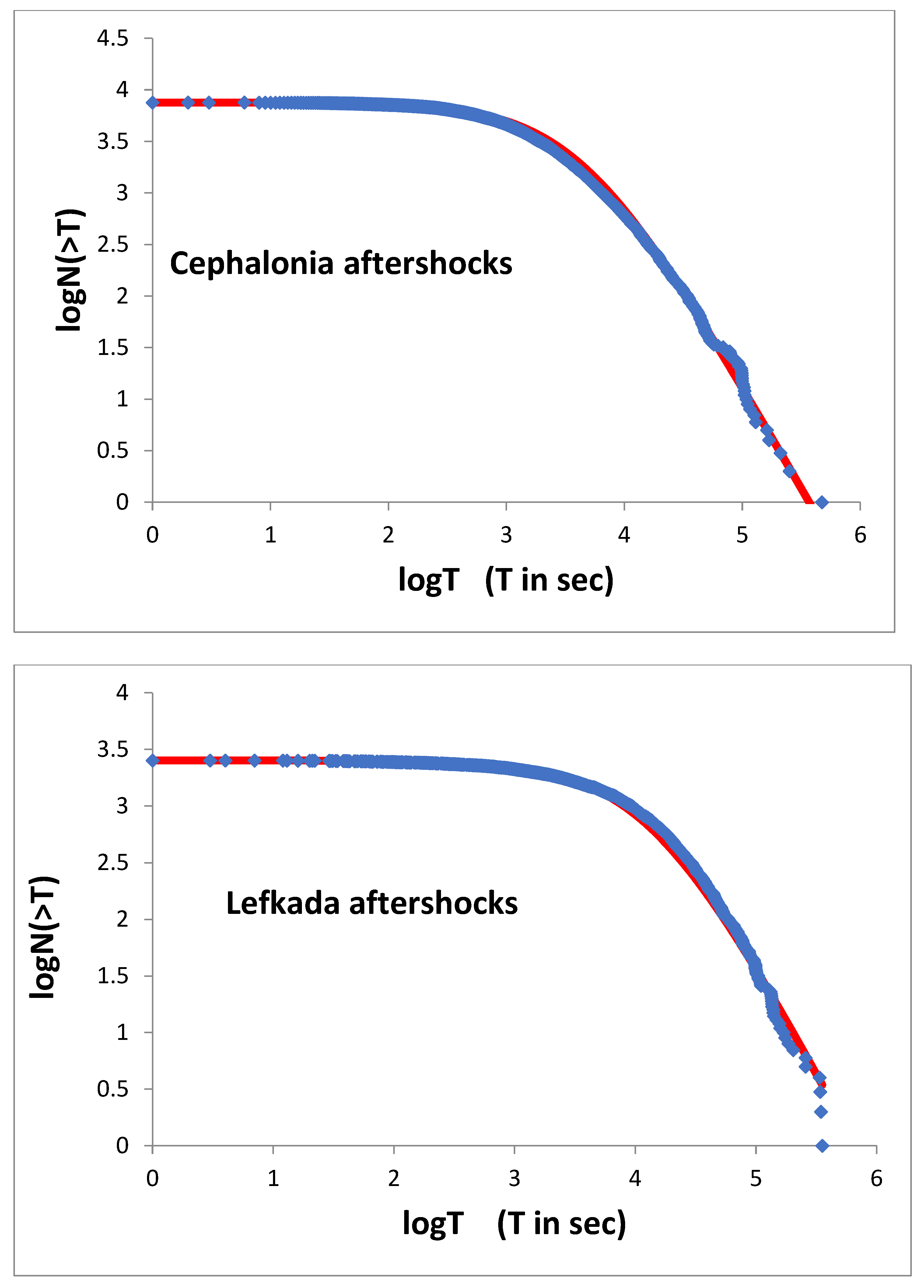
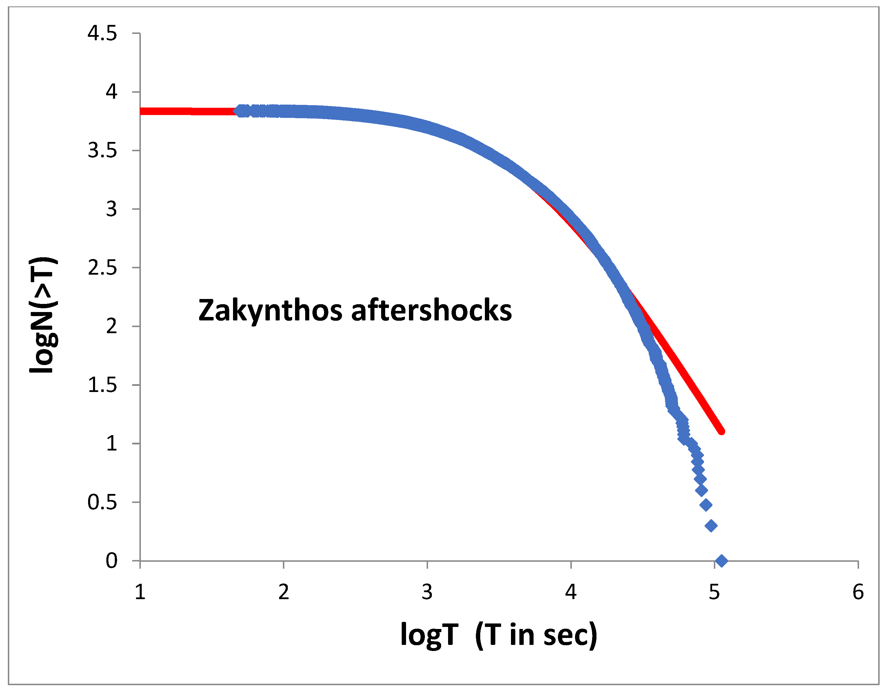
6.3. Scaling Properties of the Recent Ionian Island Aftershock Sequences in Terms of Non-Extensive Statistical Physics

Here, we explore the behavior of the recent Ionian Islands aftershock sequences in terms of non-extensive statistical physics (NESP).

The fragment–asperity model in the form of Equation (8) is fitted to the normalized cumulative number of earthquakes for the three aftershock sequences (Figure 8), with the results given in Table 2. A q_M value close to 1.5 is obtained for all three cases, in agreement with a b value close to one. Considering the RMSE values of the G–R relationship and the fragment asperity model (Table 2), these indicate that the latter provides a slightly better fit to the observed frequency–magnitude distributions.

Furthermore, we analyze the distribution of interevent times in the three aftershock sequences using NESP. The cumulative distribution function P(>T) of the aftershocks interevent times is plotted log-log in Figure 9, displaying a typical q-exponential pattern. An examination of Figure 9 shows that a departure from the q-exponential function is seen for large values of T (T > Tc, where Tc is a critical interevent interval). A visual inspection in Figure 9 suggests Tc values of the order of 1.6, 3 and 0.5 days for the Cephalonia, Lefkada and Zakynthos aftershock sequences, respectively. Additionally, a q_T = 1.50 for all three examples is obtained by fitting the q-exponential to the observed data up to a value around the deviation value Tc, in agreement with previous results [70,71,72].

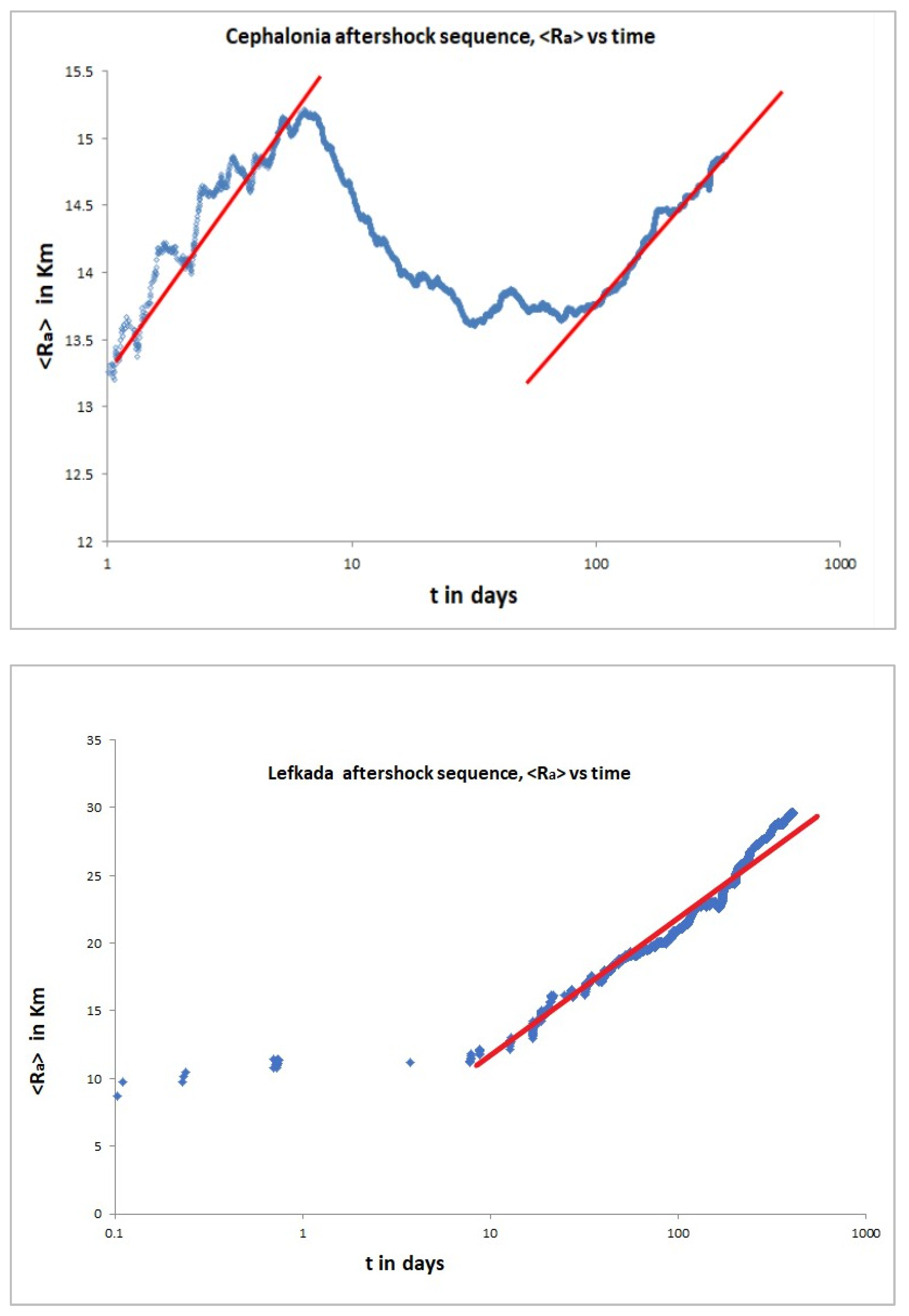
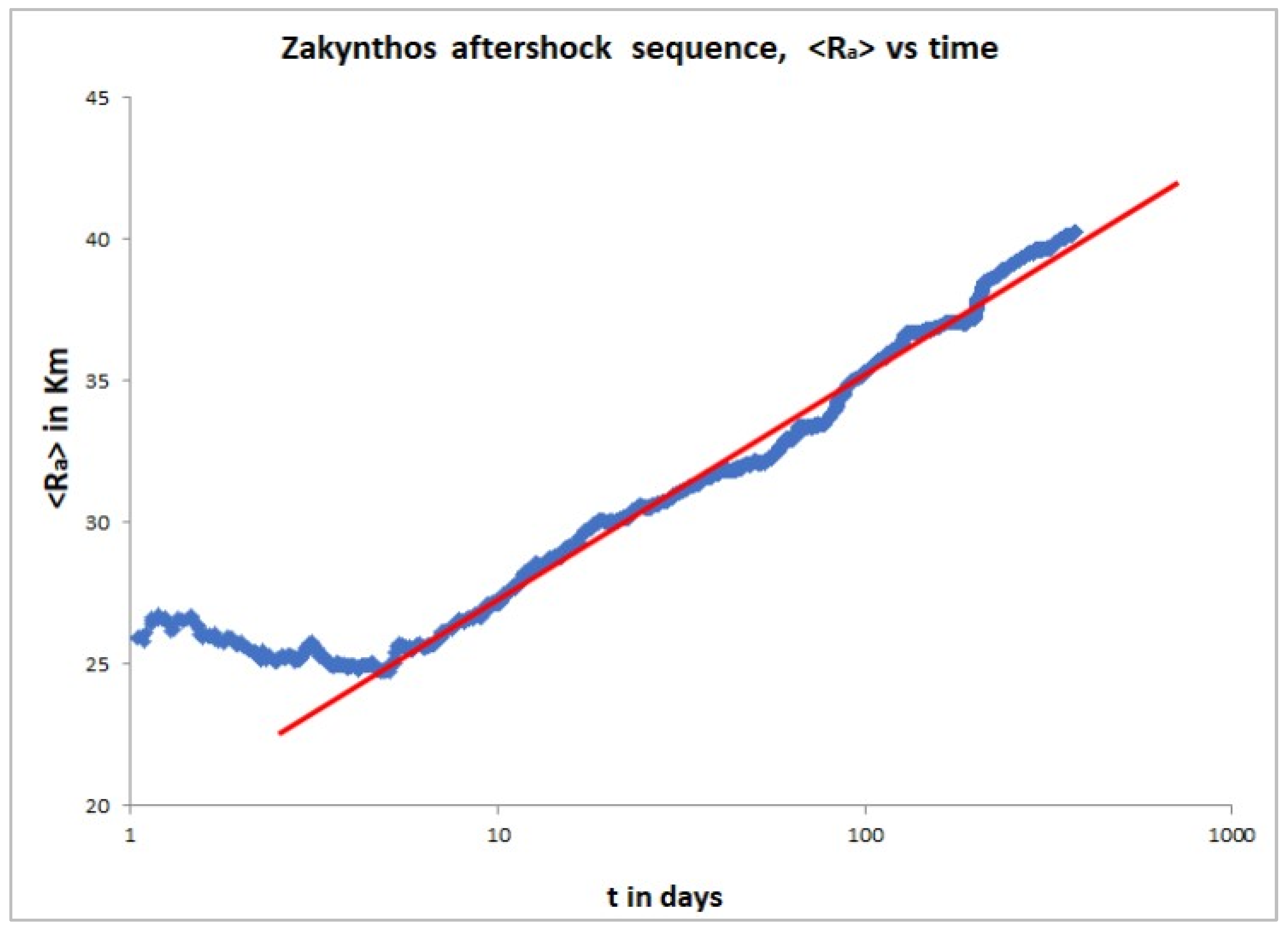
7. Scaling of Aftershock Zone with Time

Static and dynamic stresses are the main factors that govern diffusion and the spatiotemporal distribution of aftershocks [73,74,75,76,77]. Here, we explore the expansion of the aftershock zone as the logarithm of time for the three Ionian Island aftershock sequences [63,77,78,79,80,81,82,83]. This semilogarithmic migration is indicative of seismic activity following afterslip-driven aftershocks, as demonstrated by numerical simulations [84,85]. In [82] recently presented an analytical model that predicts the first-order observables of the aftershock migration and extension along the strike, as driven by the co-seismic deformation because of the main earthquake.

According to Perfettini et al. [82] and [86]’s model, aftershock development is controlled by the afterslip loading the asperities. Thus, the seismicity rate R(t) is carried out by

$$R\left(t\right)={\displaystyle \frac{R_{+}\exp \left(\raisebox{1ex}{$t$}\!\left/ \!\raisebox{-1ex}{$t_r$}\right.\right)}{1+\left(\frac{R_{+}}{R_L}\right)[exp\left(\raisebox{1ex}{$t$}\!\left/ \!\raisebox{-1ex}{$t_r$}\right.\right)-1]}}$$

(13)

where the long-term seismicity rate following the main event is denoted by R_L, the seismicity rate immediately following the end of the coseismic rupture by R+, and the duration of the postseismic phase by t_r defined as $t_r=A_1/(d\sigma /dt),\mathrm{with}$ A₁ = (a_r − b_s)σ_eff and $R_{+}=R_{L}exp\left({\displaystyle \frac{\Delta CFS}{A}}\right)$, where dσ/dt is the stressing rate, a_r and b_s are the rate and state frictional parameters, σ_eff is the effective normal stress, and ΔCFS is the Coulomb stress change brought on by the main event. Equation (13) yields an Omori regime for ${\displaystyle \raisebox{1ex}{$\mathit{t}$}\!\left/ \!\raisebox{-1ex}{${\mathit{t}}_{\mathit{r}}$}\right.}\ll 1$ with p = 1, τ = 1/$R_{+}$ and c = ${\displaystyle \frac{R_{+}}{R_L{t}_r}}$.

A fault is assumed to have a depth dependency of normal stress, stressing rate, and rheological parameter A in accordance with [82]. In order to construct the initial distribution of afterslip velocities, we additionally take into account as a first-order approximation the migration of aftershocks along the strike direction x and assume that the initial Coulomb stress field fluctuates with x. Considering the situation a few weeks after the mainshock, which permits us to assume that the postseismic relaxation is still in the early stage and the approximation t≪t_r, is valid, the aftershock zone migrates with a propagation velocity of $V_p={\displaystyle \frac{A_1}{t}}{(-{\displaystyle \frac{\partial \Delta CFS}{\partial x}})}^{-1}$ with decay as 1/t, suggesting that amongst time t₁ and t, the aftershock zone migrated by $\mathsf{\Delta }{R}_a\left(t\right)=R_a\left(t\right)-R_a\left(t_1\right)=A_1{\left(-{\displaystyle \frac{\partial \mathsf{\Delta }\mathit{C}\mathit{F}\mathit{S}}{\partial \mathit{x}}}\right)}^{-1}\mathrm{l}\mathrm{n}\left({\displaystyle \frac{t}{t_1}}\right)$, which predicts a logarithmic migration with time. The latter suggests a slow migration of the aftershock zone when a smooth coseismic Coulomb stress field exists.

In [63,82,83], order of magnitude estimates of the Coulomb stress gradient along the strike direction x are presented,

$$\mathsf{\Delta }\mathit{C}\mathit{F}\mathit{S}\left(\mathit{x}\right)=\mathsf{\Delta }\mathit{\sigma }[(1-({\displaystyle \frac{\mathit{R}}{\mathit{x}}}{)}^3{)}^{-1/2}-1]$$

(14)

for x > R, where R is the radius of the coseismic rupture and Δσ > 0 is the absolute value of the mean coseismic stress drop.

The latter approach estimates the average derivative of the Coulomb stress field in relation to the along-strike direction (x) over R and 2R as $<{\left(-{\displaystyle \frac{\partial \mathsf{\Delta }\mathit{C}\mathit{F}\mathit{S}}{\partial \mathit{x}}}\right)}^{-1}>=\mathit{\zeta }{\displaystyle \frac{\mathit{R}}{\mathsf{\Delta }\mathit{\sigma }}}$, where ζ = 2.77 as calculated in [82,86]. Thus, the average migration of the aftershock zone along the strike is provided by Equation (15).

$$<\mathsf{\Delta }{R}_a\left(t\right)>=<R_a\left(t\right)>-R_a\left(t_1\right)=A_1<{\left(-{\displaystyle \frac{\partial \mathsf{\Delta }CFS}{\partial x}}\right)}^{-1}>\ln \left({\displaystyle \frac{t}{t_1}}\right)=\zeta A_1{\displaystyle \frac{R}{\mathsf{\Delta }\sigma }}\ln \left({\displaystyle \frac{t}{t_1}}\right)$$

(15)

Starting from the first day after the mainshock and continuing over the next few months, Figure 10 shows the migration of the aftershock zone for the aftershock sequences as indicated by Equation (15). The location of the afterslip front as a function of time is in accordance with the straight lines in Figure 10, which depict the along-strike distance of after events as a function of the logarithm of time. Additionally, with a rough estimate of the average stress drop during the mainshock Δσ and the source radius R, Equation (15) might be used to determine the order of magnitude of the ${\mathit{A}}_1$ rheological parameter.

Using the equation $R={\left({\displaystyle \frac{7}{16}}{\displaystyle \frac{M_o}{\Delta \sigma }}\right)}^{1/3}$ [87], where Μo is the seismic moment represented by $M_o={10}^{1.5M_w+9}$, one may calculate the source radius R. The later expression results in $R={10}^{0.5(M_w-M_{ref})}$ where $M_{ref}={\displaystyle \frac{2}{3}}\log \left({\displaystyle \frac{16\Delta \sigma }{7}}\right)$ is the magnitude at which R = 1 km. Therefore, once the slope $s={\displaystyle \frac{d<R_a\left(t\right)>}{dlnt}}=\zeta A_1{\displaystyle \frac{R}{\Delta \sigma }}$ is determined, it can be utilized to provide a rough estimate of $A_1$.

Fitting the first days $<\mathsf{\Delta }{R}_a\left(t\right)>$ versus the logarithm of time for the Cephalonia aftershock sequence and assuming a stress drop of the order of 0.177 MPa [88] leads to a value of the rheological parameter $A_1$ of the order of 0.01 MPa, while for the Lefkada and the Zakynthos earthquakes, assuming a stress drop of the order of 5 MPa [89], the values of 1.28 and 0.71 MPa are obtained for the rheological parameter $A_1$, respectively. All the values are in agreement with the $A_1$ values in the range 0.01–1 MPa found in [63,90]. In addition, in [91], a value of $A_1$ = 0.5 MPa was estimated for the 1992 M_w 7.3 Landers earthquake, while a similar value was proposed in [86] for the 2011 M_w 9.0 Tohoku earthquake. We note that an $A_1$ value as low as that obtained for the Cephalonia event was also presented in [83] for the 2020 M_w 7.0 Samos earthquake and in [81] for the Central Chile subduction zone.

We note that for the Cephalonia aftershock sequence, a deviation from relation (18) is observed after the first days of the aftershock evolution process, possibly linked to the preparation of a significant aftershock event (see Figure 10).

8. Discussion

The present work examined the scaling characteristics of the aftershock sequences from Ionian Island that followed the three strong shallow mainshocks that occurred recently.

The scaling characteristics of the aftershock sequences are in line with established empirical aftershock relationships. In particular, the frequency–magnitude distribution of the aftershocks follows the well-known Gutenberg–Richter scaling relationship, with b-values close to 1. According to a composite model of various Omori regimes, the aftershock production rate for the three sequences decays as a power-law with time, indicating the development of secondary aftershock sequences generated by the occurrence of strong aftershock events. The interevent times between the successive aftershocks also present scaling that is well approximated by a q-exponential distribution function and a crossover behavior between Tsallis and Boltzmann Gibbs statistics observed for short and long interevent times, respectively.

A complementary approach to non-extensive statistical mechanics that further illuminate the dynamics of the interevent times distributions is the superstatistical one [92,93]. A superposition of conventional local equilibrium states, governed by an intense parameter β that varies on a relatively broad spatial-temporal scale, provides the foundation for the superstatistic interpretation of a complex system ([16,94,95] and references therein).

This view is based on a Poisson process $p\left(T|\beta \right)=\beta e^{-\beta {\rm T}}$, where the conditional probability density $p\left(T|\beta \right)$ to observe the interevent time T changes to a random variable according to the parameter β. If β is distributed with probability density f(β) and varies over a large time interval, we can obtain the marginal distribution of the interevent times

$$p\left(T\right)={\int }_0^{\infty }f\left(\beta \right)p\left(T|\beta \right)d\beta ={\int }_0^{\infty }f\left(\beta \right)\beta e^{-\beta {\rm T}}d\beta$$

(16)

In this case, the probability density of β is given by a x²-distribution with n degrees of freedom:

$$f\left(\beta \right)={\displaystyle \frac{1}{\Gamma \left(n/2\right)}}{\left({\displaystyle \frac{n}{2{\beta }_0}}\right)}^{n/2}{\beta }^{{\displaystyle \frac{n}{2}}-1}exp\left(-{\displaystyle \frac{n\beta }{2{\beta }_0}}\right)$$

(17)

where Γ(n/2) is the Gamma function [93].

The integral (16) is easily evaluated [93] and one obtains $p\left(T\right)\approx C{\left(1+B\left(q-1\right)T\right)}^{1/\left(1-q\right)}$, which is exactly the result obtained in the frame of NESP, where $q=1+[2/\left(n+2\right)]$, $B={\displaystyle \frac{2{\beta }_0}{2-q}}$ with β_ο the average value of β, given as $〈\beta 〉={\int }_0^{\infty }\beta f\left(\beta \right)d\beta ={\beta }_0$.

From the previous, we can estimate the degrees of freedom that are influencing the value of β by $n={\displaystyle \frac{2}{q-1}}-2$, which describes the temporal evolution of seismicity by using the q_T value of the interevent times calculated for each aftershock sequence.

In order to analyze the observed deviation from the q-exponential function, we follow the approach suggested in [70,71]. For T > Tc, the interevent time distribution can be represented by an exponential function (i.e., q = 1, in Tsallis entropy terms), while for interevent times T < Tc, the distribution is governed by Tsallis entropy. Following the differential equation pathway for the representation of non extensive statistical physics [24] the nonlinear differential equation equation ${\displaystyle \frac{dp}{dT}}=-\beta p^q$ can be solved to yield the generalized probability distribution which is given by Equation (6), associated with interevent times T < Tc. The anomalous equilibrium distribution is generalized using this differential equation path, incorporating a crossover from anomalous (q ≠ 1) to normal (q = 1) statistical mechanics, while increasing the interevent time T. Following [24,94,96], we introduce the differential equation, ${\displaystyle \frac{dp}{dT}}=-{\beta }_{1}p-\left({\beta }_q-{\beta }_1\right)p^q$ which has the solution

$$p(T)=C[1-{\displaystyle \frac{{\beta }_q}{{\beta }_1}}+{\displaystyle \frac{{\beta }_q}{{\beta }_1}}{e}^{\left(q-1\right){\beta }_{1}T}{]}^{-{\displaystyle \raisebox{1ex}{$1$}\!\left/ \!\raisebox{-1ex}{$q-1$}\right.}}$$

(18)

where C is a normalization factor and β_q and β₁ are parameters that control the evolution of the process and the transition point where T description transferred from q-exponential to an exponential function.

As T increases, p(T) reduces monotonically for positive β_q and β₁. It can be easily verified that Tc = 1/(q − 1)β₁ is the cross-over point between the non-additive and additive behavior. In the case where (q − 1)β₁ << 1, Equation (18) is approximated by p(T) ≈ C exp_q(−T/T_q) where T_q = 1/β_q which is a q-exponential function, while for (q − 1)β₁ >> 1, the asymptotic behavior of the probability distribution is the exponential function $p\left(T\right)\propto ({\displaystyle \frac{{\beta }_1}{{\beta }_q}}{)}^{{\displaystyle \raisebox{1ex}{$1$}\!\left/ \!\raisebox{-1ex}{$(q-1)$}\right.}}{e}^{-{\beta }_{1}T}$.

According to our observed data, the q-exponential distribution of interevent times for T < Tc is induced by the superstatistical model by a straightforward mechanism: a χ² distribution allocated parameter β of the local Poisson process. The distribution of interevent times in the Ionian Island aftershock sequences can be explained by this process. In accordance with [70,71], we estimate n ≈ 2 by using the observed distributions (see Figure 9) and the q-value of q_T = 1.50 obtained from our q-statistics fits. This indicates that the number of freedom degrees affecting the β value is extremely small and consistent across all situations. We observe that a high number of degrees of freedom is linked to the observed exponential functions for T > Tc. The latter suggests that the Tsallis entropic mechanism predominates during the early aftershock period when most interevent times have T values less than Tc. However, as time passes, the aftershock sequence’s characteristics, such as finite degrees of freedom and long-range memory, associated with a NESP description, cease to predominate and the Boltzmann–Gibbs (BG) statistical physics is restored (i.e., q = 1).

The latter seems to be a universal characteristic since it has been observed in a number of aftershock sequences in different geotectonic environments [70,71,72].

The spatial distribution of aftershocks as a measure of postseismic relaxation was studied. The aftershock sequence is driven by the co-seismic static stress changes caused by the mainshock, as seen by the aftershocks’ spatial distribution spreading along stress-enhanced locations. Nonetheless, the logarithmic aftershock migration over time indicates that afterslip after the primary rupture may very well be the driving force behind aftershocks. The latter gives a preliminary estimate of the fault’s rheological parameter ${\mathit{A}}_1$ in terms of rate strengthening rheology [82], which controls the evolution of the afterslip process. This estimate agrees with values estimated in other tectonic zones and laboratory tests [63,90].

According to power laws governing the distributions of seismic energy release and the temporal occurrence of aftershocks, the results given here generally confirm the self-similar character of the aftershock-generating process during the Ionian Island aftershock cycles. As a result of co-seismic stress changes and afterslip after the mainshock, aftershocks primarily migrate along the fault strikes in the spatial domain during the early post-seismic relaxation phase. Moreover, following the initial days of the aftershock evolution process, a departure from the logarithmic migration of aftershocks with time is noted for the Cephalonia aftershock sequence, which may be related to the preparation of a significant major aftershock event. Seismic hazard assessment, risk mitigation, and aftershock occurrence models can all be constrained by these features and the resultant parameters.

9. Concluding Remarks

Summarizing, in the present work the observed scaling properties in the three aftershock sequences of the recent strong earthquakes that occurred in the Ionian Island region are analysed. The frequency–magnitude distributions in terms of the Gutenberg–Richter scaling relationship are demonstrated, where a b-value close to one is estimated for all the cases. Furthermore, the temporal evolution of the aftershock sequences, as described by the Omori–Utsu expression, is tested. Since breaks appear in the cumulative number of aftershocks for all three aftershock sequences following the occurrence of moderately sized events, indicating the triggering of secondary sequences, a superposition of Omori regimes is introduced for all three aftershock sequences.

The application of non-extensive statistical physics in the interevent time distribution indicates a system in an anomalous equilibrium with long-range interactions and a cross-over behavior from anomalous to classical statistical mechanics for greater interevent times, with a common entropic parameter q_T demonstrating that aftershock sequences are systems with very low degrees of freedom.

Finally, we apply a model for the evolution of the afterslip process which results in a scaling of the migration of aftershock zones as a function of the logarithm of time, as can be observed. The departure from the logarithmic migration of aftershocks with time observed during the first days of the Cephalonia aftershock sequence may be related to the preparation of a significant second major aftershock event.

Our results contribute to the understanding of the spatiotemporal evolution of aftershocks using a first principles approach based on non-extensive statistical physics suggesting that this view could describe the process within a universal view.

References

1. Ganas, A.; Cannavò, F.; González, P.J.; Drakatos, G. The Geodetic Signature of the January 26, 2014 Earthquake Onshore Kefalonia, Greece. Unpublished Report 2014. Available online: https://www.gein.noa.gr/Documents/pdf/VLSM_co-seismic_26-1-2014_13_55_UTC.pdf (accessed on 20 September 2024).
2. Valkaniotis, S.; Ganas, A.; Papathanassiou, G.; Papanikolaou, M. Field observations of geological effects triggered by the January–February 2014 Kefalonia (Ionian Sea, Greece) earthquakes. Tectonophysics 2014, 630, 150–157. [Google Scholar] [CrossRef]
3. Papadimitriou, E.; Karakostas, V.; Mesimeri, M.; Chouliaras, G.; Kourouklas, C. The M6.7 17 November 2015 Lefkada (Greece) earthquake: Structural interpretation by means of aftershock analysis. Pure Appl. Geophys. 2017, 174, 3869–3888. [Google Scholar] [CrossRef]
4. Papadimitriou, P.; Kapetanidis, V.; Karakonstantis, A.; Spingos, I.; Pavlou, K.; Kaviris, G.; Kassaras, I.; Sakkas, V.; Voulgaris, N. The 25 October 2018 Zakynthos (Greece) earthquake: Seismic activity at the transition between a transform fault and a subduction zone. Geophys. J. Int. 2021, 225, 15–36. [Google Scholar] [CrossRef]
5. Papazachos, B.C.; Papazachou, C.B. The Earthquakes of Greece; Ziti Publications: Thessaloniki, Greece, 2003; p. 304. [Google Scholar]
6. Kiratzi, A.; Langston, C. Moment tensor inversion of the January 17, 1983 Kefallinia event of Ionian Islands. Geophys. J. Int. 1991, 105, 529–535. [Google Scholar] [CrossRef]
7. Tzanis, A.; Vallianatos, F.; Makropoulos, K. Seismic and electrical precursors to the 17-1-1983, M7 Kefallinia earthquake, Greece: Signatures of a SOC system. Phys. Chem. Earth Part A Solid Earth Geod. 2000, 25, 281–287. [Google Scholar] [CrossRef]
8. Papadimitriou, E. Mode of strong earthquake recurrence in the central Ionian Islands (Greece): Possible triggering due to Coulomb stress changes generated by the occurrence of previous strong shocks. Bull. Seismol. Soc. Am. 2002, 92, 3293–3308. [Google Scholar] [CrossRef]
9. Karakostas, V.; Papadimitriou, E.; Mesimeri, M.; Gkarlaouni, C.; Paradisopoulou, P. The 2014 Kefalonia doublet (Mw6.1 and Mw6.0), Central Ionian Islands, Greece: Seismotectonic implications along the Kefalonia transform fault zone. ActaGeophysica 2014, 63, 1–16. [Google Scholar] [CrossRef]
10. Utsu, T. A statistical study on the occurrence of aftershocks. Geophys. 1961, 30, 521–605. [Google Scholar]
11. Gutenberg, B.; Richter, C.F. Frequency of Earthquakes in California. Bull. Seismol. Soc. Am. 1944, 34, 185–188. [Google Scholar] [CrossRef]
12. Bak, P.; Tang, C. Earthquakes as a self-organized critical phenomenon. J. Geophys. Res. Solid Earth 1989, 94, 15635–15637. [Google Scholar] [CrossRef]
13. Rundle, J.B.; Turcotte, D.L.; Shcherbakov, R.; Klein, W.; Sammis, C. Statistical physics approach to understanding the multiscale dynamics of earthquake fault systems. Rev. Geophys. 2003, 41, 1019. [Google Scholar] [CrossRef]
14. Sornette, D. Critical Phenomena in Natural Sciences; Springer: Berlin/Heidelberg, Germany, 2000. [Google Scholar]
15. Vallianatos, F.; Papadakis, G.; Michas, G. Generalized statistical mechanics approaches to earthquakes and tectonics. Proc. R. Soc. A 2016, 472, 20160497. [Google Scholar] [CrossRef]
16. Vallianatos, F.; Chatzopoulos, G. A Complexity View into the Physics of the Accelerating Seismic Release Hypothesis: Theoretical Principles. Entropy 2018, 20, 754. [Google Scholar] [CrossRef] [PubMed]
17. Telesca, L.; Lapenna, V.; Vallianatos, F. Monofractal and multifractal approaches in investigating scaling properties in temporal patterns of the 1983–2000 seismicity in the western Corinth graben, Greece. Phys. Earth Planet. Int. 2002, 131, 63–79. [Google Scholar] [CrossRef]
18. Telesca, L.; Macchiato, M. Time-scaling properties of the Umbria-Marche 1997–1998 seismic crisis, investigated by the detrended fluctuation analysis of interevent time series Chaos. Solitons Fractals 2004, 19, 377–385. [Google Scholar] [CrossRef]
19. Vallianatos, F.; Michas, G.; Papadakis, G. A description of seismicity based on non-extensive statistical physics: A review. In Earthquakes and Their Impact on Society; D’Amico, S., Ed.; Springer Natural Hazards: Heidelberg, Germany, 2016; pp. 1–42. [Google Scholar] [CrossRef]
20. Papadakis, G.; Vallianatos, F.; Sammonds, P. Evidence of Nonextensive Statistical Physics behavior of the Hellenic Subduction Zone seismicity. Tectonophysics 2013, 608, 1037–1048. [Google Scholar] [CrossRef]
21. Davidsen, J.; Goltz, C. Are seismic waiting time distributions universal? Geophys. Res. Lett. 2004, 31, L21612. [Google Scholar] [CrossRef]
22. Corral, Á.; Christensen, K. Comment on “earthquakes descaled: On waiting time distributions and scaling laws”. Phys. Rev. Lett. 2006, 96, 109801. [Google Scholar] [CrossRef] [PubMed]
23. Michas, G.; Vallianatos, F.; Sammonds, P. Non-extensivity and long-range correlations in the earthquake activity at the West Corinth rift (Greece). Nonlin. Processes Geophys. 2013, 20, 713–724. [Google Scholar] [CrossRef]
24. Tsallis, C. Introduction to Nonextensive Statistical Mechanics: Approaching a Complex World; Springer: Berlin/Heidelberg, Germany, 2009; ISBN 978-0-387-85358-1. [Google Scholar] [CrossRef]
25. Kokinou, E.; Papadimitriou, E.; Karakostas, V.; Kamberis, V.; Vallianatos, F. The Kefalonia Transform Zone (offshore Western Greece) with special emphasis to its prolongation towards the Ionian Abyssal Plain. Mar. Geophys. Res. 2006, 27, 241–252. [Google Scholar] [CrossRef]
26. Scordilis, E.; Karakaisis, G.; Karakostas, V.; Panagiotopoulos, D.; Comninakis, P.; Papazachos, B.C. Evidence for transform faulting in the Ionian Sea: The Kefalonia Island earthquake sequence of 1983. Pure Appl. Geophys. 1985, 123, 388–397. [Google Scholar] [CrossRef]
27. Sachpazi, M.; Hirn, A.; Clement, C.; Haslinger, F.; Laigle, M.; Kissling, E.; Charvis, P.; Hello, Y.; Lepine, J.C.; Sapin, M.; et al. Western Hellenic subduction and Kefalonia Transform: Local earthquakes and plate transport and strain. Tectonophysics 2000, 319, 301–319. [Google Scholar] [CrossRef]
28. Le Pichon, X.; Lallemant, S.J.; Chamot-Rooke, N.; Lemeur, D.; Pascal, G. The Mediterranean Ridge backstop and the Hellenic nappes. Mar. Geol. 2002, 186, 111–125. [Google Scholar] [CrossRef]
29. Hollenstein, C.; Müller, M.D.; Geiger, A.; Kahle, H.G. Crustal motion and deformation in Greece from a decade of GPS measurements, 1993–2003. Tectonophysics 2008, 449, 17–40. [Google Scholar] [CrossRef]
30. Papazachos, C.B.; Kiratzi, A. A detailed study of the active crustal deformation in the Aegean and surrounding area. Tectonophysics 1996, 253, 129–153. [Google Scholar] [CrossRef]
31. Louvari, E.; Kiratzi, A.; Papazachos, B.C. The Cephalonia Transform Fault and its extension to western Lefkada island (Greece). Tectonophysics 1999, 308, 223–236. [Google Scholar] [CrossRef]
32. Makropoulos, K.; Kaviris, G.; Kouskouna, V. An extended earthquake catalogue for Greece and adjacent areas since 1900, enriched with the Mw addition. Nat. Hazards Earth Syst. Sci. 2012, 12, 1425–1430. [Google Scholar] [CrossRef]
33. Bonatis, P.; Karakostas, V.G.; Papadimitriou, E.E.; Kaviris, G. Investigation of the Factors Controlling the Duration and Productivity of Aftershocks Following Strong Earthquakes in Greece. Geosciences 2022, 12, 328. [Google Scholar] [CrossRef]
34. Evangelidis, C.P.; Triantafyllis, N.; Samios, M.; Boukouras, K.; Kontakos, K.; Ktenidou, O.J.; Fountoulakis, I.; Kalogeras, I.; Melis, N.S.; Galanis, O.; et al. Seismic Waveform Data from Greece and Cyprus: Integration, Archival, and Open Access. Seismol. Res. Lett. 2021, 92, 1672–1684. [Google Scholar] [CrossRef]
35. Klein, F.W. Users guide to HYPOINVERSE-2000: A Fortran Program to Solve for Earthquake Locations and Magnitudes. U.S. Geol. Surv. Open-File Rept. 02-171, Version 1.0. 2002. Available online: https://pubs.usgs.gov/of/2002/0171/pdf/of02-171.pdf (accessed on 20 September 2024).
36. Papadimitriou, P.; Chousianitis, K.; Agalos, A.; Moshou, A.; Lagios, E.; Makropoylos, K. The spatially extended 2006 April Zakynthos (Ionian Islands, Greece) seismic sequence and evidence for stress transfer. Geophys. J. Int. 2012, 191, 1025–1040. [Google Scholar] [CrossRef]
37. Xiong, X.; Shan, B.; Zhou, Y.M.; Wei, S.J.; Li, Y.D.; Wang, R.; Zheng, Y. Coulomb stress transfer and accumulation on the Sagaing Fault, Myanmar, over the past 110 years and its implications for seismic hazard. Geophys.Res. Lett. 2017, 44, 4781–4789. [Google Scholar] [CrossRef]
38. Wu, J.; Hu, Q.; Li, W.; Lei, D. Study on Coulomb Stress Triggering of the April 2015 M7.8 Nepal Earthquake Sequence. Int. J. Geophys. 2016, 2016, 7378920. [Google Scholar] [CrossRef]
39. Mayorga, E.F.; Sánchez, J.J. Modelling of Coulomb stress changes during the great (Mw=8.8) 1906 Colombia-Ecuador earthquake. J. South Am. Earth Sci. 2016, 70, 268–278. [Google Scholar] [CrossRef]
40. Kilb, D.; Gomberg, J.; Bodin, P. Aftershock triggering by complete Coulomb stress changes. JGR Solid Earth 2002, 107, ESE 2-1–ESE 2-14. [Google Scholar] [CrossRef]
41. Stein, R.S. The role of stress transfer in earthquake occurrence. Nature 1999, 402, 605–609. [Google Scholar] [CrossRef]
42. King, G.C.; Stein, R.; Lin, J. Static stress changes and the triggering of earthquakes. Bull. Seismol. Soc. Am. 1994, 84, 935–953. [Google Scholar] [CrossRef]
43. Toda, S.; Stein, R.S.; Richards-Dinger, K.; Bozkurt, S.B. Forecasting the evolution of seismicity in southern California: Animations built on earthquake stress transfer. J. Geophys. Res. 2005, 110, 1–17. [Google Scholar] [CrossRef]
44. Toda, S.; Stein, R.S.; Sevilgen, V.; Lin, J. Coulomb 3.3 Graphic-Rich Deformation and Stress-Change Software for Earthquake, Tectonic, and Volcano Research and Teaching-User Guide. U.S. Geological Survey Open-File Report 2011-1060. 2011; p. 63. Available online: http://pubs.usgs.gov/of/2011/1060/ (accessed on 20 September 2024).
45. Kilb, D.; Gomberg, J.; Bodin, P. Triggering of earthquake aftershocks by dynamic stresses. Nature 2002, 408, 570–574. [Google Scholar] [CrossRef] [PubMed]
46. Cattania, C.; Hainzl, S.; Wang, L.; Roth, F.; Enescu, B. Propagation of Coulomb stress uncertainties in physics-based aftershock models. J. Geophys. Res. 2014, 119, 7846–7864. [Google Scholar] [CrossRef]
47. Sokos, E.; Kiratzi, A.; Gallovič, F.; Zahradník, J.; Serpetsidaki, A.; Plicka, V. Rupture process of the 2014 Cephalonia, Greece, earthquake doublet (Mw6) as inferred from regional and local seismic data. Tectonophysics 2015, 656, 131–141. [Google Scholar] [CrossRef]
48. Papadimitriou, P.; Karakonstantis, A.; Bozionelos, G.; Kapetanidis, V.; Kaviris, G.; Spingos, I.; Millas, C. Preliminary Report on the Lefkada 17 November 2015 Mw=6.4 Earthquake, Report Released to EMSC-CSEM. 2016. Available online: https://www.emsc-csem.org/Doc/Additional_Earthquake_Report/470390/20151117_lefkada_report_nkua.pdf (accessed on 20 September 2024).
49. Harris, R.A. Introduction to special section: Stress triggers, stress shadows, and implications for seismic hazard. J. Geophys. Res. 1998, 103, 347–358. [Google Scholar] [CrossRef]
50. Beeler, N.; Simpson, R.; Hickman, S.; Lockner, D. Pore fluid pressure, apparent friction, and Coulomb failure. J. Geophys. Res. 2000, 105, 25533–25542. [Google Scholar] [CrossRef]
51. Rice, J.; Cleary, M. Some basic stress diffusion solutions for fluid saturated elastic porous media with compressible constituents. Rev. Geophys. 1976, 14, 227–241. [Google Scholar] [CrossRef]
52. Bonatis, P.; Karakostas, V.; Papadimitriou, E.; Kouroukla, C. The 2022 Mw5.5 earthquake off-shore Kefalonia Island—Relocated aftershocks, statistical analysis and seismotectonic implications. J. Seismol. 2024, 1–17. [Google Scholar] [CrossRef]
53. Kourouklas, C.; Papadimitriou, E.; Karakostas, V. Long-Term Recurrence Pattern and Stress Transfer along the Kefalonia Transform Fault Zone (KTFZ), Greece: Implications in Seismic Hazard Evaluation. Geosciences 2023, 13, 295. [Google Scholar] [CrossRef]
54. Gutenberg, B.; Richter, C.F. Magnitude and energy of earthquakes. Ann. Geofis 1954, 9, 1–15. [Google Scholar] [CrossRef]
55. Frohlich, C.; Davis, S.D. Teleseismic b values; Or, much ado about 1.0. J. Geophys. Res. Solid Earth 1993, 98, 631–644. [Google Scholar] [CrossRef]
56. Scholz, C. The Mechanics of Earthquakes and Faulting, 3rd ed.; Cambridge University Press: Cambridge, UK, 2019. [Google Scholar]
57. Kisslinger, C. Aftershocks and fault-zone properties. Adv. Geophys. 1996, 38, 1–36. [Google Scholar] [CrossRef]
58. Utsu, T. A statistical significance test of the difference in b-value between two earthquakes groups. J. Phys. Earth 1966, 14, 37–40. [Google Scholar] [CrossRef]
59. Shi, Y.; Bolt, B.A. The standard error of the magnitude-frequency b-value. Bull. Seismol. Soc. Am. 1982, 87, 1074–1077. [Google Scholar] [CrossRef]
60. Wiemer, S.; Wyss, M. Minimum magnitude of complete reporting in earthquake catalogs: Examples from Alaska, the Western United States, and Japan. Bull. Seismol. Soc. Am. 2000, 90, 859–869. [Google Scholar] [CrossRef]
61. Utsu, T.; Ogata, Y.; Matsu’ura, R.S. The centenary of the Omori formula for a decay law of aftershock activity. J. Phys. Earth 1995, 43, 1–33. [Google Scholar] [CrossRef]
62. Ogata, Y. Estimation of the parameters in the modified Omori formula for aftershock frequencies by the maximum likelihood procedure. J. Phys. Earth. 1983, 31, 115–124. [Google Scholar] [CrossRef]
63. Michas, G.; Pavlou, K.; Avgerinou, S.E.; Anyfadi, E.A.; Vallianatos, F. Aftershock patterns of the 2021 Mw 6.3 Northern Thessaly (Greece) earthquake. J. Seismol. 2022, 26, 201–225. [Google Scholar] [CrossRef]
64. Tsallis, C. Nonadditive entropy and nonextensive statistical mechanics—An overview after 20 years. Braz. J. Phys. 2009, 39, 337–356. [Google Scholar] [CrossRef]
65. Tsallis, C. Possible Generalization of Boltzmann-Gibbs Statistics. J. Stat. Phys. 1988, 52, 479–487. [Google Scholar] [CrossRef]
66. Silva, R.; Franca, G.S.; Vilar, C.S.; Alcaniz, J.S. Nonextensive models for earthquakes. Phys. Rev. E 2006, 73, 026102. [Google Scholar] [CrossRef]
67. Telesca, L. Investigating the temporal variations of the time-clustering behavior of the Koyna–Warna (India) reservoir-triggered seismicity, Chaos. Solitons Fractals 2011, 44, 108–113. [Google Scholar] [CrossRef]
68. Telesca, L. Maximum likelihood estimation of the nonextensive parameters of the earthquake cumulative magnitude distribution. Bull. Seismol. Soc. Am. 2012, 102, 886–891. [Google Scholar] [CrossRef]
69. Abe, S.; Suzuki, N. Scale-free statistics of time interval between successive earthquakes. Phys. A 2005, 350, 588–596. [Google Scholar] [CrossRef]
70. Avgerinou, S.E.; Anyfadi, E.A.; Michas, G.; Vallianatos, F.A. Non-Extensive Statistical Physics View of the Temporal Properties of the Recent Aftershock Sequences of Strong Earthquakes in Greece. Appl. Sci. 2023, 13, 1995. [Google Scholar] [CrossRef]
71. Anyfadi, E.A.; Avgerinou, S.E.; Michas, G.; Vallianatos, F. Universal Non-Extensive Statistical Physics Temporal Pattern of Major Subduction Zone Aftershock Sequences. Entropy 2022, 24, 1850. [Google Scholar] [CrossRef]
72. Vallianatos, F.; Karakonstantis, A.; Michas, G.; Pavlou, K.; Kouli, M.; Sakkas, V. On the Patterns and Scaling Properties of the 2021–2022 Arkalochori Earthquake Sequence (Central Crete, Greece) Based on Seismological, Geophysical and Satellite Observations. Appl. Sci. 2022, 12, 7716. [Google Scholar] [CrossRef]
73. Lippiello, E.; Giacco, F.; Marzocchi, W.; Godano, C.; de Arcangelis, L. Mechanical origin of aftershocks. Sci. Rep. 2015, 5, 15560. [Google Scholar] [CrossRef]
74. Helmstetter, A.; Sornette, D. Diffusion of epicenters of earthquake aftershocks, Omori’s law, and generalized continuous-time random walk models. Phys. Rev. E 2002, 66, 061104. [Google Scholar] [CrossRef] [PubMed]
75. Felzer, K.R.; Brodsky, E.E. Decay of aftershock density with distance indicates triggering by dynamic stress. Nature 2006, 441, 735–738. [Google Scholar] [CrossRef] [PubMed]
76. Lippiello, E.; de Arcangelis, L.; Godano, C. Role of Static Stress Diffusion in the Spatiotemporal Organization of Aftershocks. Phys. Rev. Lett. 2009, 103, 038501. [Google Scholar] [CrossRef] [PubMed]
77. Kato, A.; Obara, K. Step-like migration of early aftershocks following the 2007 Mw 6.7 Noto-Hanto earthquake, Japan. Geophys. Res. Lett. 2014, 41, 3864–3869. [Google Scholar] [CrossRef]
78. Obana, K.; Takahashi, T.; No, T.; Kaiho, Y.; Kodaira, S.; Yamashita, M.; Sato, T.; Nakamura, T. Distribution and migration of aftershocks of the 2010 Mw 7.4 Ogasawara Islands intraplate normal-faulting earthquake related to a fracture zone in the Pacific plate. Geochem. Geophys. Geosyst. 2014, 15, 1363–1373. [Google Scholar] [CrossRef]
79. Tang, C.C.; Lin, C.H.; Peng, Z. Spatial-temporal evolution of early aftershocks following the 2010 ML6.4 Jiashian earthquake in southern Taiwan. Geophys. J. Int. 2014, 199, 1772–1783. [Google Scholar] [CrossRef]
80. Meng, X.; Peng, Z. Increasing lengths of aftershock zones with depths of moderate-size earthquakes on the San Jacinto Fault suggests triggering of deep creep in the middle crust. Geophys. J. Int. 2016, 204, 250–261. [Google Scholar] [CrossRef]
81. Frank, W.B.; Poli, P.; Perfettini, H. Mapping the rheology of the Central Chile subduction zone with aftershocks. Geophys. Res. Lett. 2017, 44, 5374–5382. [Google Scholar] [CrossRef]
82. Perfettini, H.; Frank, W.B.; Marsan, D.; Bouchon, M.A. Model of Aftershock Migration Driven by Afterslip. Geophys. Res. Lett. 2018, 45, 2283–2293. [Google Scholar] [CrossRef]
83. Vallianatos, F.; Pavlou, K. Scaling properties of the Mw7.0 Samos (Greece), 2020 aftershock sequence. Acta Geophy. 2021, 69, 1067–1084. [Google Scholar] [CrossRef]
84. Ariyoshi, K.; Matsuzawa, T.; Hasegawa, A. The key frictional parameters controlling spatial variations in the speed of postseismic-slip propagation on a subduction plate boundary. Earth Planet. Sci. Lett. 2007, 256, 136–146. [Google Scholar] [CrossRef]
85. Kato, N. Expansion of aftershock areas caused by propagating post-seismic sliding. Geophys. J. Int. 2007, 168, 797–808. [Google Scholar] [CrossRef]
86. Perfettini, H.; Avouac, J.P. Postseismic relaxation driven by brittle creep: A possible mechanism to reconcile geodetic measurements and the decay rate of aftershocks, application to the Chi-Chi earthquake, Taiwan. J. Geophys. Res. Solid Earth 2004, 109, 1–25. [Google Scholar] [CrossRef]
87. Kanamori, H.; Anderson, D.L. Theoretical basis of some empirical relations in seismology. Bull. Seismol. Soc. Am. 1975, 65, 1073–1095. [Google Scholar] [CrossRef]
88. Dologlou, E. Critical dynamic processes prior to destructive earthquakes. Int. J. Remote Sens. 2014, 35, 8208–8216. [Google Scholar] [CrossRef]
89. Margaris, B.; Hatzidimitriou, P. Source spectral scaling and stress release estimates using strong-motion records in Greece. Bull. Seismol. Soc. Am. 2002, 92, 1040–1059. [Google Scholar] [CrossRef]
90. Perfettini, H.; Avouac, J.P.; Tavera, H.; Kositsky, A.; Nocquet, J.M.; Bondoux, F.; Chlieh, M.; Sladen, A.; Audin, L.; Farber, L.; et al. Seismic and aseismic slip on the Central Peru megathrust. Nature 2010, 465, 78–81. [Google Scholar] [CrossRef]
91. Perfettini, H.; Avouac, J.P. Modeling afterslip and aftershocks following the 1992 Landers earthquake. J. Geophys. Res. 2007, 112, B07409. [Google Scholar] [CrossRef]
92. Beck, C.; Cohen, E.G.D. Superstatistics. Phys. A Stat. Mech. Its Appl. 2003, 322, 267–275. [Google Scholar] [CrossRef]
93. Beck, C. Recent developments in superstatistics. Braz. J. Physics 2009, 39, 357–363. [Google Scholar] [CrossRef]
94. Vallianatos, F. A non-extensive statistical physics approach to the polarity reversals of the geomagnetic field. Phys. A 2011, 390, 1773–1778. [Google Scholar] [CrossRef]
95. Vallianatos, F.; Karakostas, V.; Papadimitriou, E. A Non-Extensive Statistical Physics View in the Spatiotemporal Properties of the 2003 (Mw6.2) Lefkada, Ionian Island Greece, Aftershock Sequence. Pure Appl. Geophys. 2014, 171, 1343–1534. [Google Scholar] [CrossRef]
96. Vallianatos, F.; Sammonds, P. Evidence of non-extensive statistical physics of the lithospheric instability approaching the 2004 Sumatran–Andaman and 2011 Honshu mega-earthquakes. Tectonophysics 2013, 590, 52–58. [Google Scholar] [CrossRef]
Figure 1. Background seismicity of strong events located within the study area. Earthquakes before and after 1900 are indicated by gradient purple and green stars, respectively (the lighter colors indicate older events than the darker ones). Also, the beach balls illustrate the focal mechanisms of recent strong earthquakes. (Source www.gein.noa.gr and www.geol.uoa.gr, accessed on 20 February 2024).
Geosciences 15 00084 g001
Figure 2. Aftershocks and fault plane solutions map for the three aftershock sequences. Red focal mechanisms indicate the three main strong earthquakes, while with yellow color the focal mechanisms of Zakynthos aftershocks (thrust faults). Green and orange colors mark the dextral strike-slip fault plane solutions in Cephalonia and Lefkada aftershock sequences, respectively.
Geosciences 15 00084 g002
Figure 3. Coulomb stress changes (ΔCFS) determined on the rupture fault plane of the 2014 Mw 6.1 Cephalonia earthquake in focal depth. Purple lines and light purple circles illustrate the faults and the aftershocks, respectively, while the red rectangle is the fault, and the green is its projection onto the earth’s surface.
Geosciences 15 00084 g003
Figure 4. Coulomb stress changes (ΔCFS) determined on the rupture fault plane of the 2015 Mw 6.4 Lefkada earthquake in focal depth. Purple lines and light purple circles illustrate the faults and the aftershocks, respectively.
Geosciences 15 00084 g004
Figure 5. Coulomb stress changes (ΔCFS) determined on the rupture fault plane of the 2018 Zakynthos Mw 6.7 earthquake in focal depth. Purple lines and light purple circles illustrate the faults and the aftershocks, respectively.
Geosciences 15 00084 g005
Figure 6. Frequency–magnitude distributions for the studied aftershock sequences, (a) Cephalonia, (b) Lefkada and (c) Zakynthos. Symbols represent the cumulative (circles) and the discrete number of earthquakes (triangles). Solid lines represent the G–R relationship for M ≥ Mc (filled circles) and for the parameter values specified in Table 2.
Geosciences 15 00084 g006aGeosciences 15 00084 g006b
Figure 7. The cumulative number of aftershocks (symbols) (with M ≥ Mc) with time that followed the three strong earthquakes in the Ionian islands: (a) Cephalonia, (b) Lefkada and (c) Zakynthos. The solid line represents the composite model of several modified Omori regimes. Vertical dashed lines mark the initiation times of secondary aftershock sequences considered in the composite model.
Geosciences 15 00084 g007
Figure 8. Normalized frequency–magnitude distributions (symbols) for the studied aftershock sequences: (a) Cephalonia, (b) Lefkada and (c) Zakynthos. Solid lines represent the fragment–asperity model (see Equation (8)) for MMc and for the parameter values given in Table 2. The dashed line indicates the 95% confidence interval.
Geosciences 15 00084 g008
Figure 9. The cumulative distribution function of the interevent times T for the Cephalonia, Lefkada and Zakynthos aftershock sequences (from top to bottom). The red solid line represents the q-exponential function fitted to the data.
Geosciences 15 00084 g009aGeosciences 15 00084 g009b
Figure 10. Aftershock zone average migration as function of the logarithm of time for the three recent aftershock sequences in the Ionian Islands, starting from the first day following the mainshock. The correlation coefficient for Cephalonia, Lefkada and Zakynthos aftershock sequences is 0.94, 0.97 and 0.985, respectively.
Geosciences 15 00084 g010aGeosciences 15 00084 g010b