
Modeling Flood Susceptibility Utilizing Advanced Ensemble Machine Learning Techniques in the Marand Plain


Abstract
1. Introduction
2. Materials and Methodology
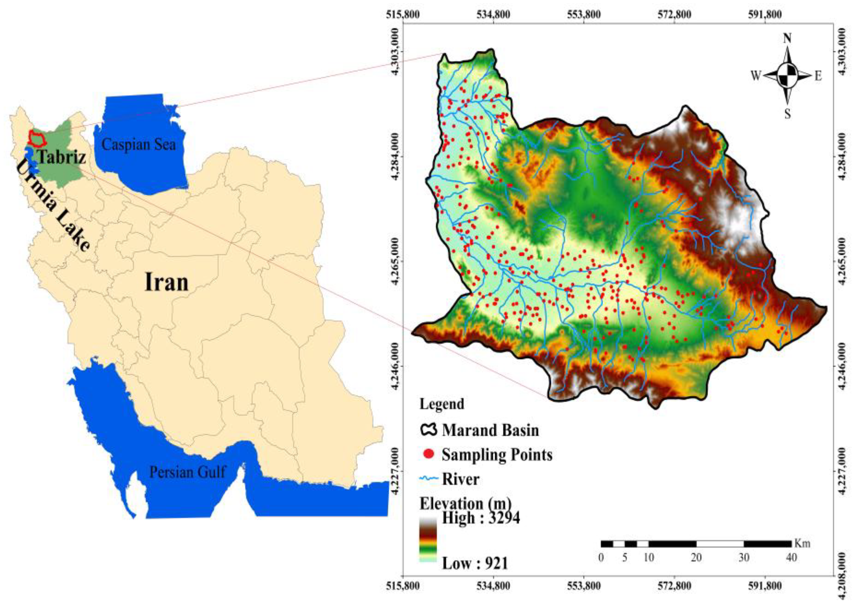
2.1. Description of the Case Study
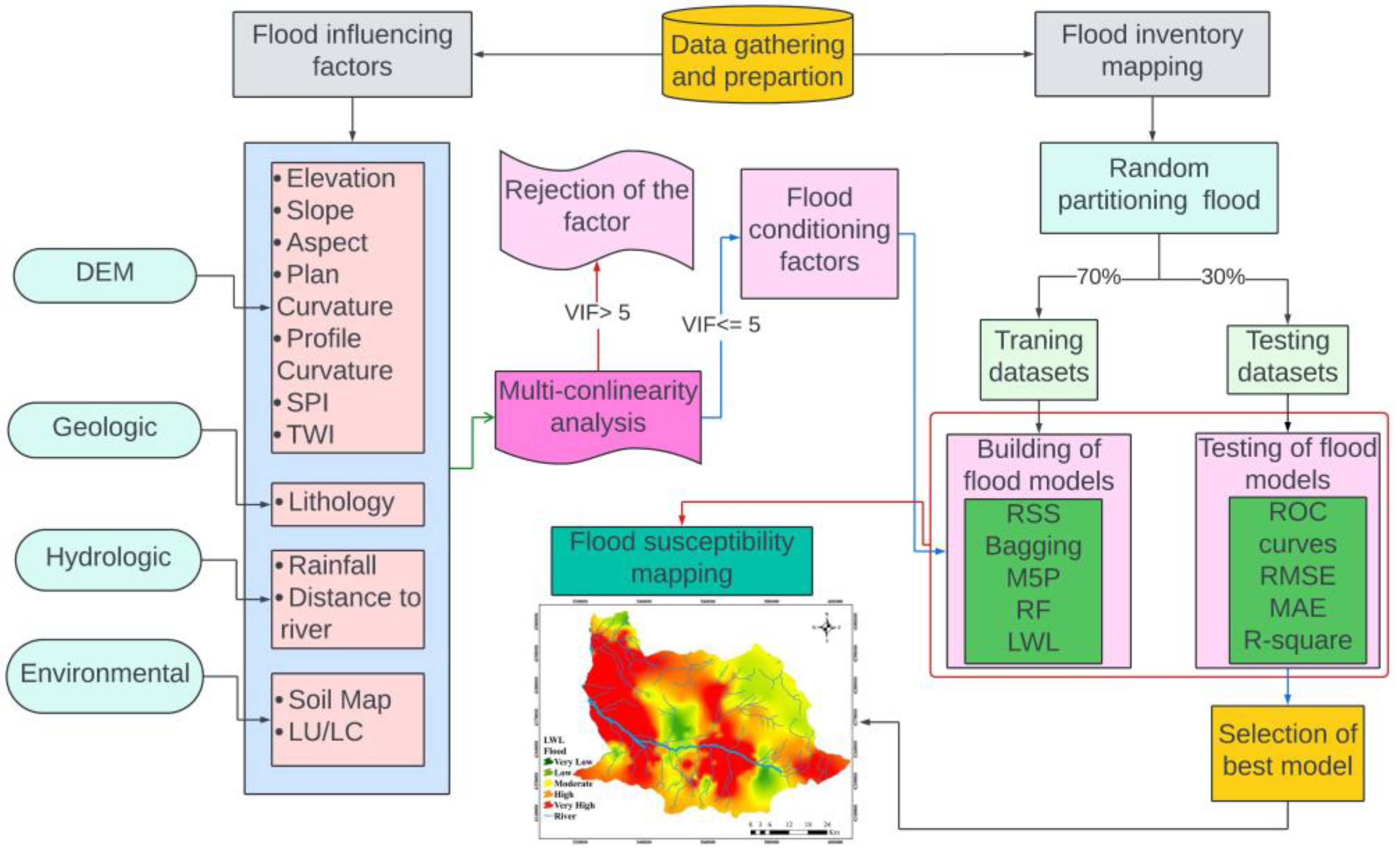
2.2. Methodology
2.2.1. Flood Inventory
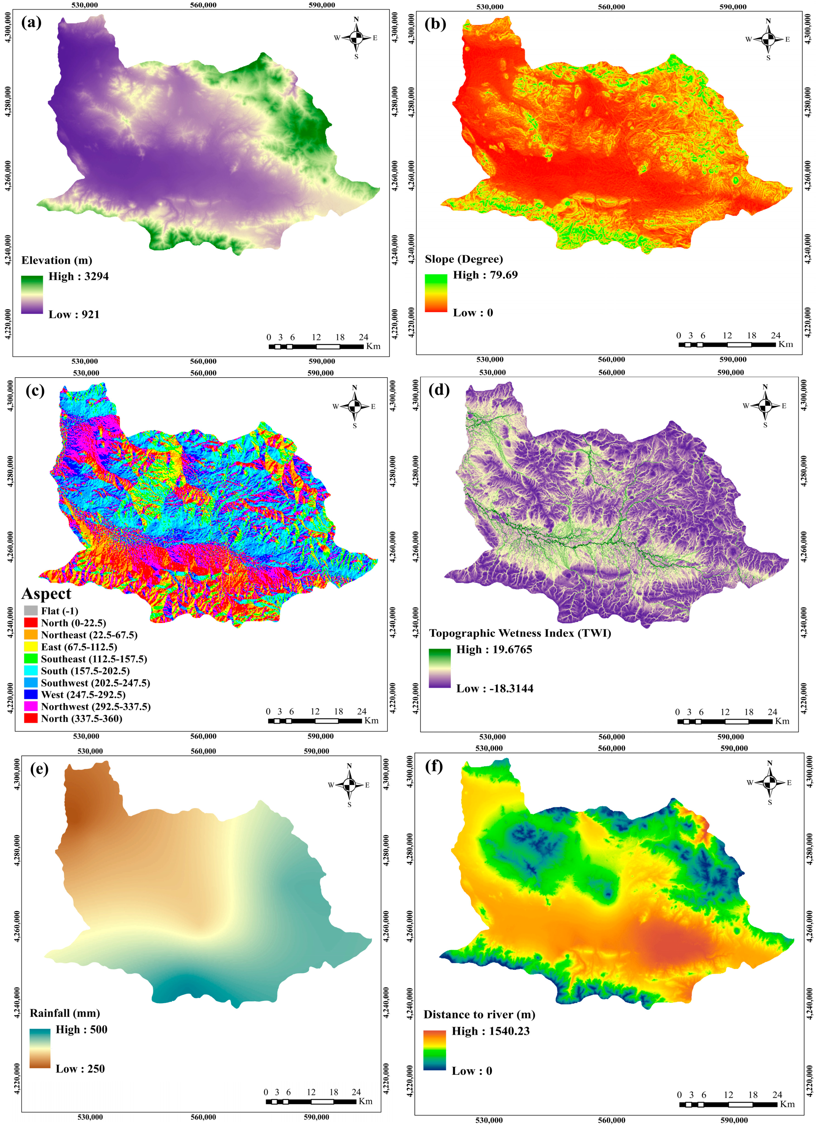
2.2.2. Flood Influencing Factors
Elevation
Slope
Aspect
Topographic Wetness Index (TWI)
Precipitation
Distance to River
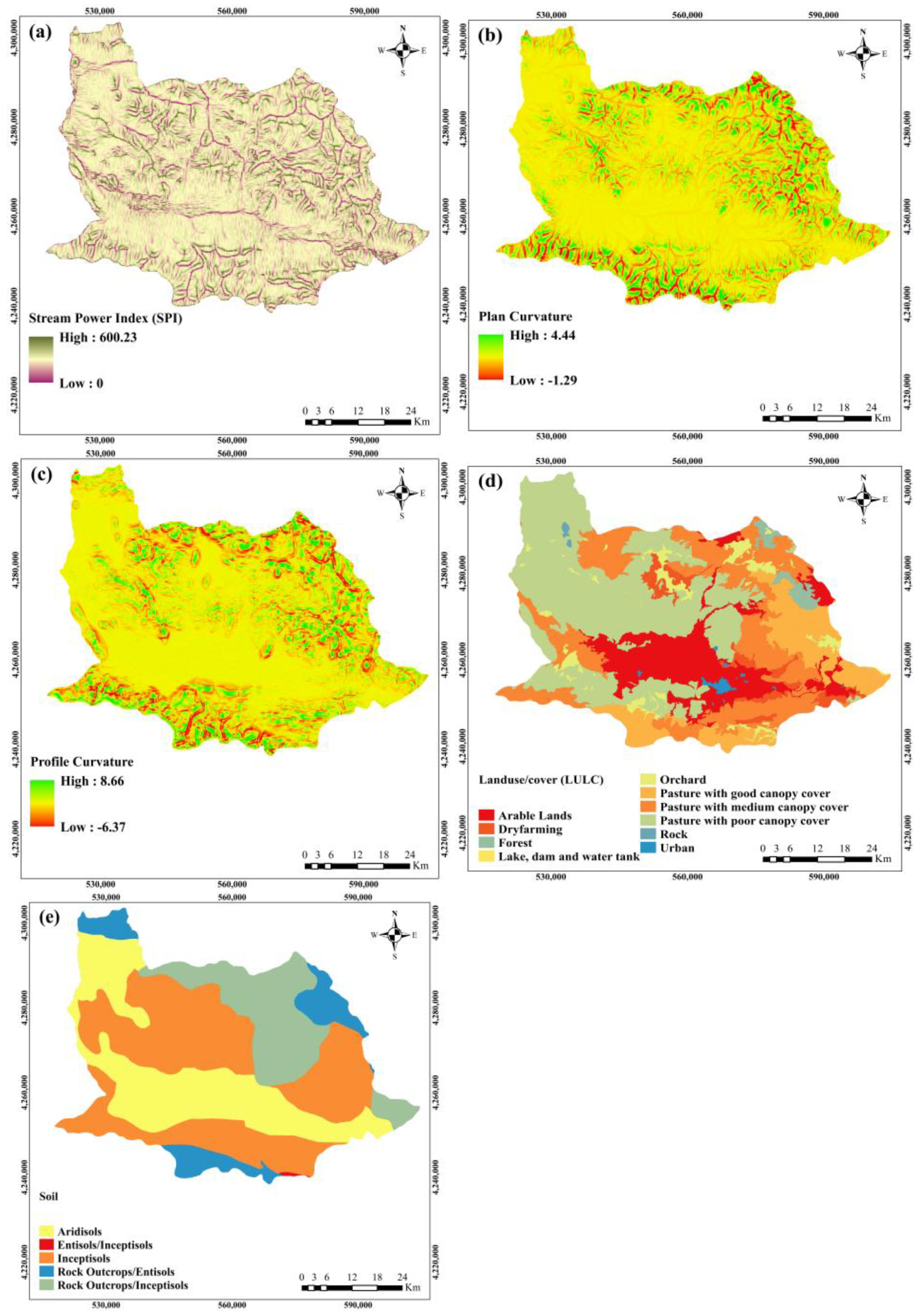
Stream Power Index (SPI)
Curvature
Land Use/Cover
Soil
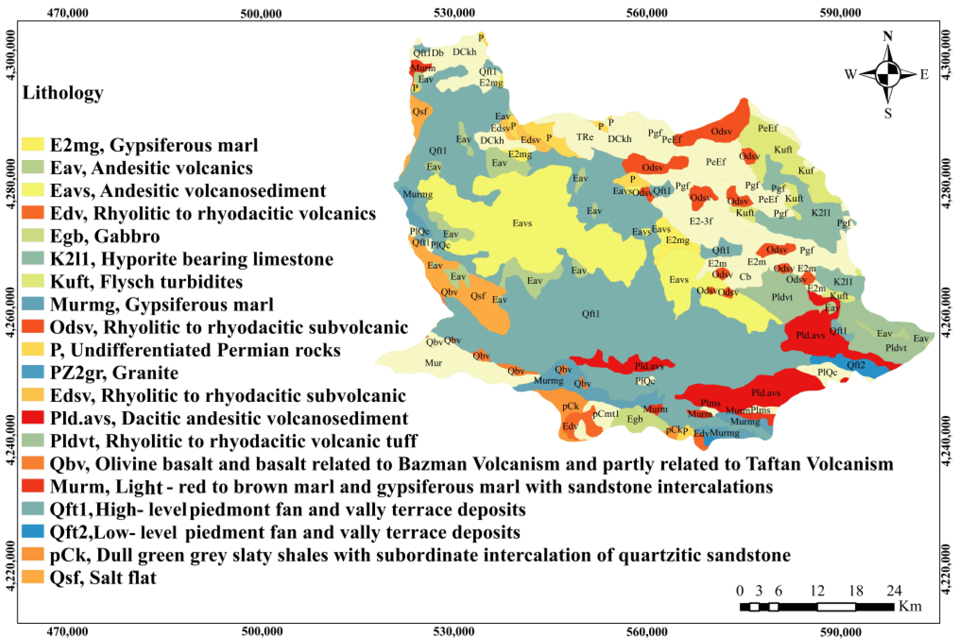
Lithology
2.3. Flood Modeling Methods
2.3.1. Random Forest (RF)
2.3.2. Random SubSpace Method (RSS)
2.3.3. Bagging
2.3.4. M5P Model Tree Algorithm (M5P)
2.3.5. Locally Weighted Learning (LWL)
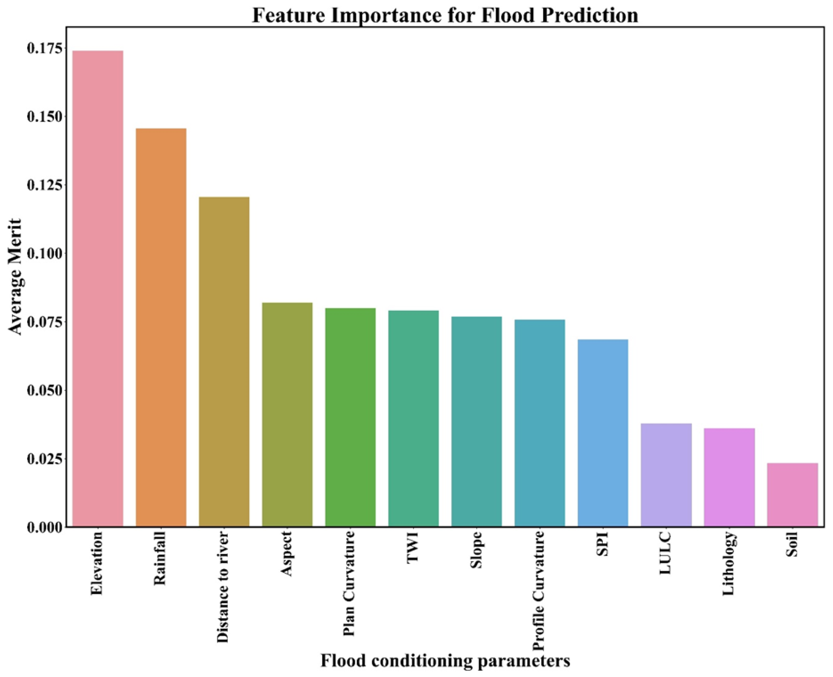
2.4. Investigating Flood Influencers via Information Gain Ratio and Multicollinearity Methodologies
2.5. Evaluation of Models Performance
3. Results
3.1. Flood Influential Factors
3.2. Overview of Flood Parameters
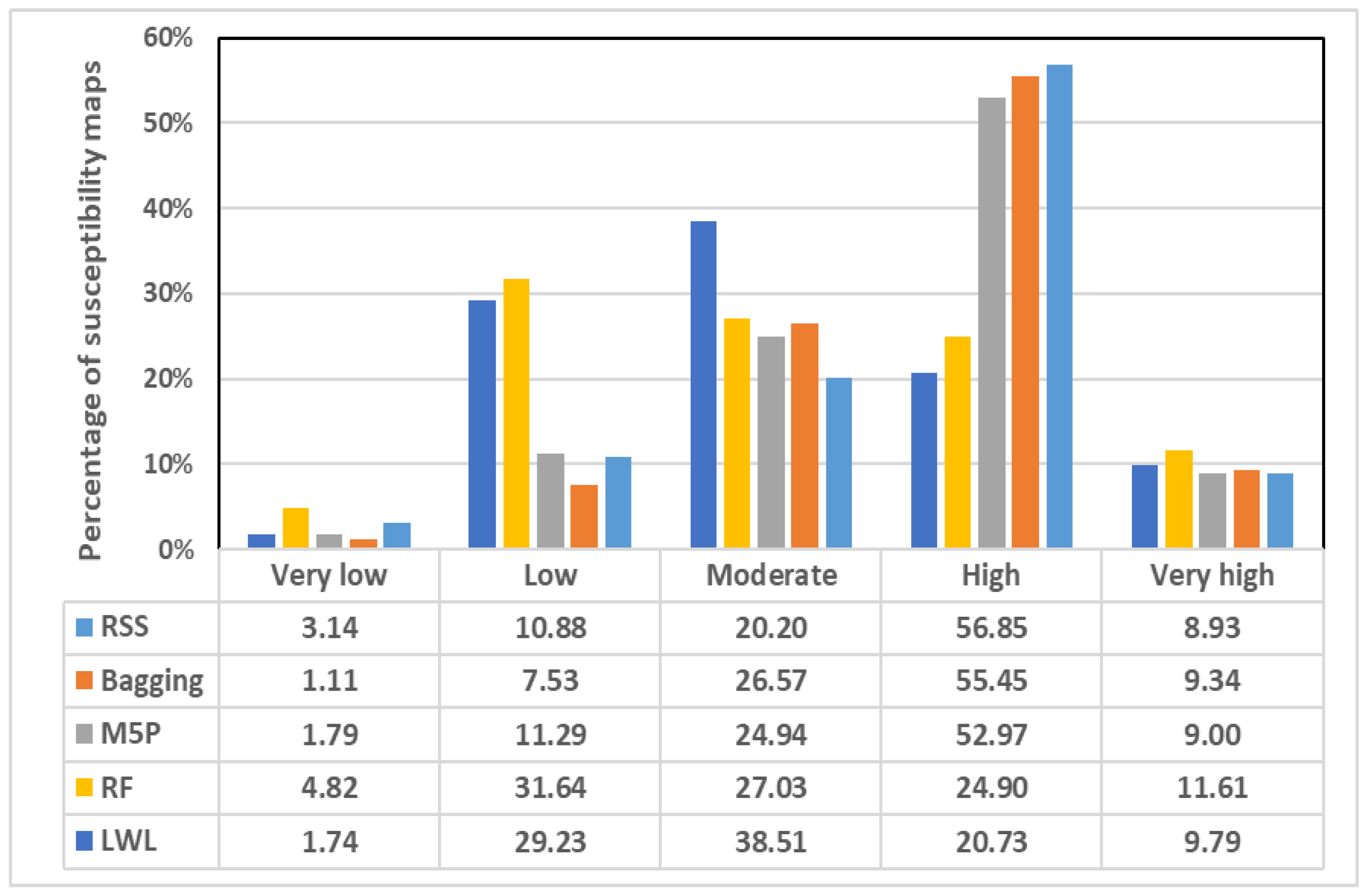
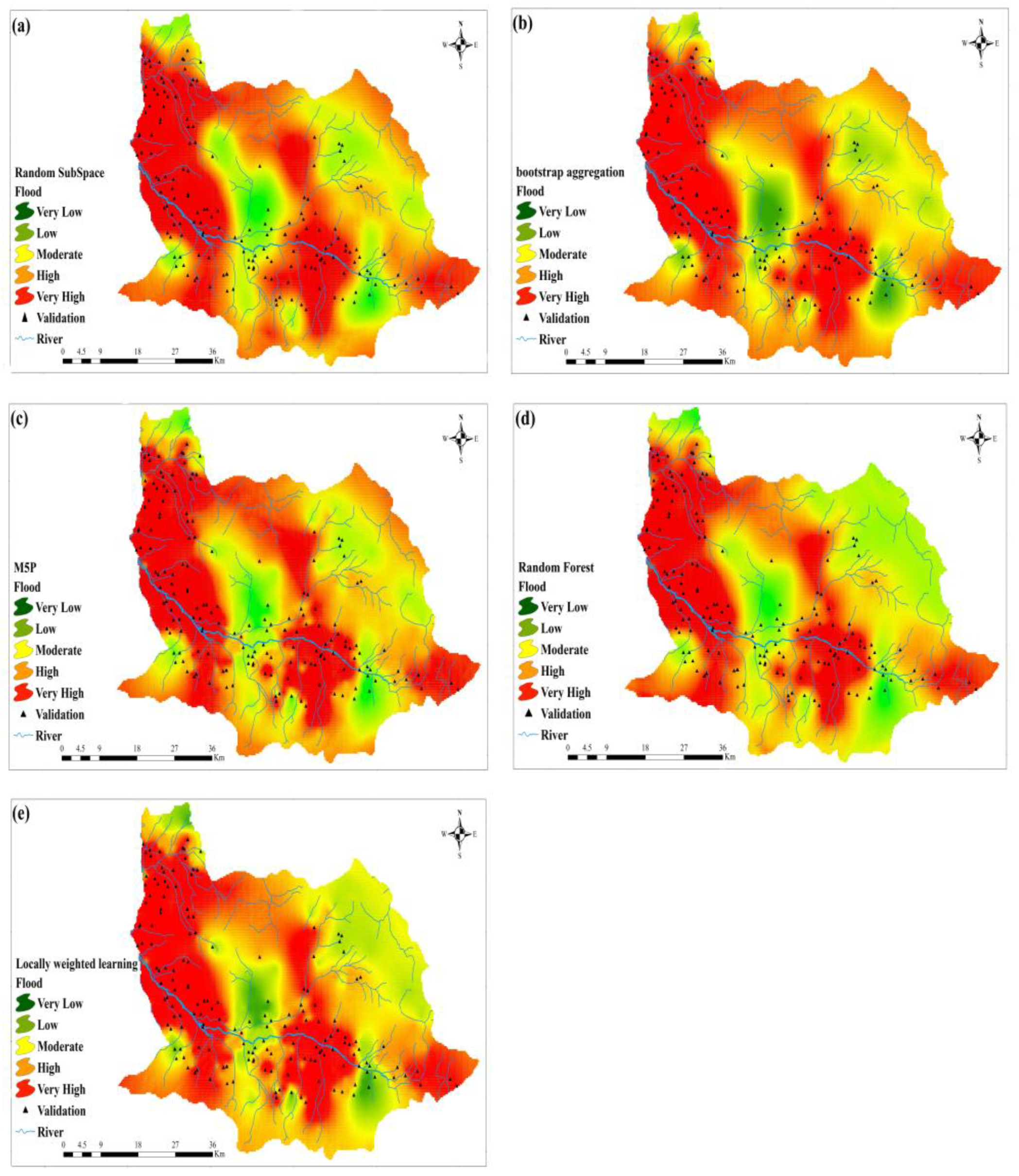
3.3. Assessment of Flood Risk Models
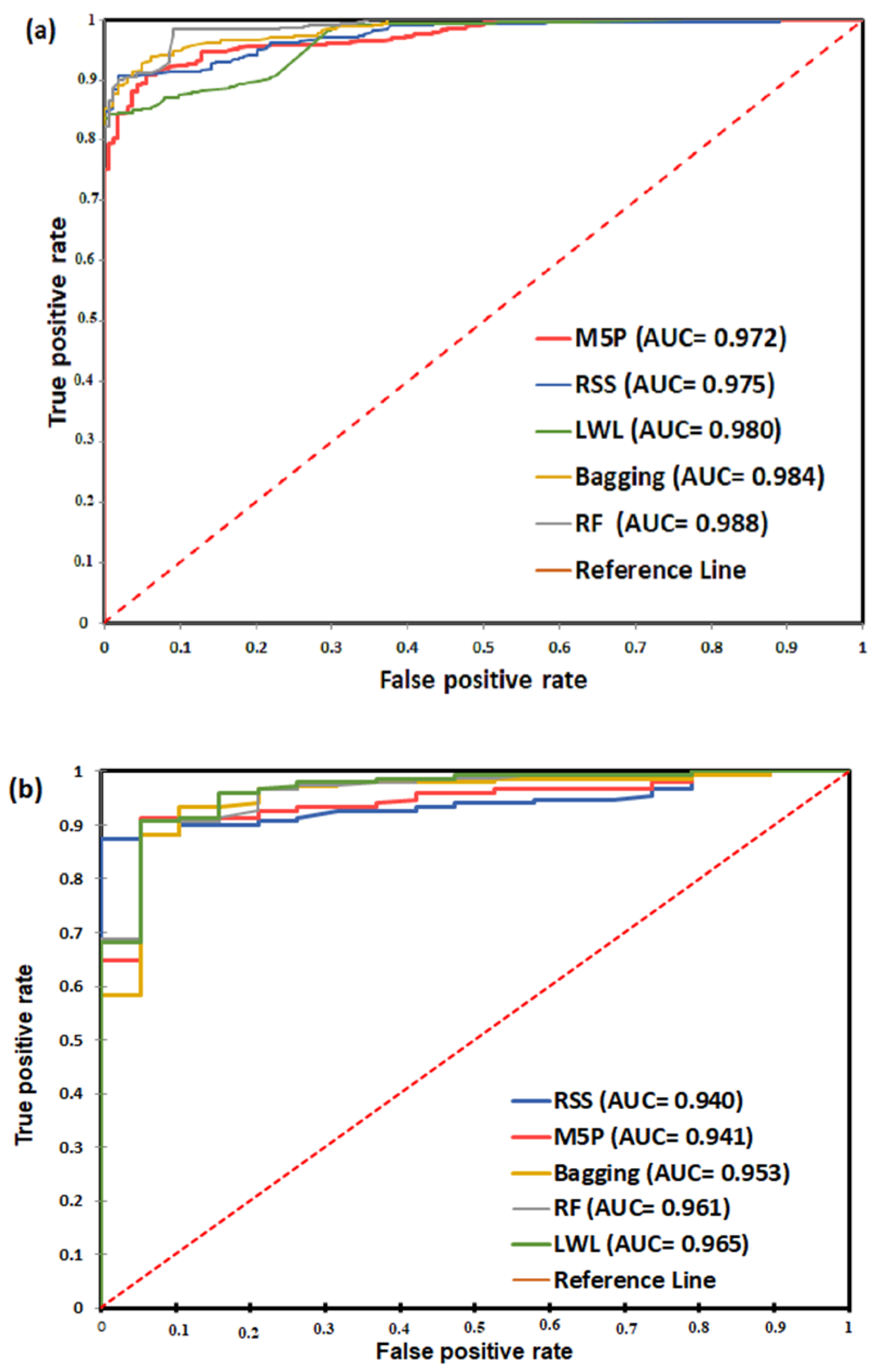
3.4. Evaluation and Validation of Models
4. Discussion
4.1. Evaluating Uncertainties in Hydrological Modeling
4.2. Impacts of Flood Variability on the Modeling Processes
4.3. Human Interventions in Flood Management
5. Conclusions
Author Contributions
Funding
Data Availability Statement
Conflicts of Interest
References
- Mousavi, S.M.; Rostamzadeh, H. Estimation of flood land use/land cover mapping by regional modelling of flood hazard at sub-basin level case study: Marand basin. Geomat. Nat. Hazards Risk 2019, 10, 1155–1175. [Google Scholar] [CrossRef]
- Pradhan, B.; Lee, S.; Dikshit, A.; Kim, H. Spatial flood susceptibility mapping using an explainable artificial intelligence (XAI) model. Geosci. Front. 2023, 14, 101625. [Google Scholar] [CrossRef]
- UNISDR. Global Assessment Report on Disaster Risk Reduction. International Strategy for Disaster Reduction (ISDR); UNISDR: Geneva, Switzerland, 2011. [Google Scholar]
- Islam, A.R.M.T.; Talukdar, S.; Mahato, S.; Kundu, S.; Eibek, K.U.; Pham, Q.B.; Kuriqi, A.; Linh, N.T.T. Flood susceptibility modelling using advanced ensemble machine learning models. Geosci. Front. 2021, 12, 101075. [Google Scholar] [CrossRef]
- Jahandideh-Tehrani, M.; Zhang, H.; Helfer, F.; Yu, Y. Review of climate change impacts on predicted river streamflow in tropical rivers. Environ. Monit. Assess. 2019, 191, 752. [Google Scholar] [CrossRef] [PubMed]
- Rahmati, O.; Kornejady, A.; Samadi, M.; Nobre, A.D.; Melesse, A.M. Development of an automated GIS tool for reproducing the HAND terrain model. Environ. Model. Softw. 2018, 102, 1–12. [Google Scholar] [CrossRef]
- Vaghefi, S.A.; Keykhai, M.; Jahanbakhshi, F.; Sheikholeslami, J.; Ahmadi, A.; Yang, H.; Abbaspour, K.C. The future of extreme climate in Iran. Sci. Rep. 2019, 9, 1464. [Google Scholar] [CrossRef]
- Shokri, A.; Sabzevari, S.; Hashemi, S.A. Impacts of flood on health of Iranian population: Infectious diseases with an emphasis on parasitic infections. Parasite Epidemiol. Control 2020, 9, e00144. [Google Scholar] [CrossRef]
- Alborzi, A.; Zhao, Y.; Nazemi, A.; Mirchi, A.; Mallakpour, I.; Moftakhari, H.; Ashraf, S.; Izadi, R.; AghaKouchak, A. The tale of three floods: From extreme events and cascades of highs to anthropogenic floods. Weather. Clim. Extrem. 2022, 38, 100495. [Google Scholar] [CrossRef]
- Shahabi, H.; Shirzadi, A.; Ghaderi, K.; Omidvar, E.; Al-Ansari, N.; Clague, J.J.; Geertsema, M.; Khosravi, K.; Amini, A.; Bahrami, S.; et al. Flood detection and susceptibility mapping using sentinel-1 remote sensing data and a machine learning approach: Hybrid intelligence of bagging ensemble based on k-nearest neighbor classifier. Remote Sens. 2020, 12, 266. [Google Scholar] [CrossRef]
- Habibian, F. Increased number of floods in Iran. WWW Document. Econ. News Database 2018. [Google Scholar]
- Dodangeh, E.; Choubin, B.; Eigdir, A.N.; Nabipour, N.; Panahi, M.; Shamshirband, S.; Mosavi, A. Integrated machine learning methods with resampling algorithms for flood susceptibility prediction. Sci. Total Environ. 2020, 705, 135983. [Google Scholar] [CrossRef] [PubMed]
- Razavi, S.; Gober, P.; Maier, H.R.; Brouwer, R.; Wheater, H. Anthropocene flooding: Challenges for science and society. Hydrol. Process. 2020, 34, 1996–2000. [Google Scholar] [CrossRef]
- Gharakhanlou, N.M.; Perez, L. Flood susceptible prediction through the use of geospatial variables and machine learning methods. J. Hydrol. 2023, 617, 129121. [Google Scholar] [CrossRef]
- Shafizadeh-Moghadam, H.; Valavi, R.; Shahabi, H.; Chapi, K.; Shirzadi, A. Novel forecasting approaches using combination of machine learning and statistical models for flood susceptibility mapping. J. Environ. Manag. 2018, 217, 1–11. [Google Scholar] [CrossRef] [PubMed]
- Bera, S.; Das, A.; Mazumder, T. Evaluation of machine learning, information theory and multi-criteria decision analysis methods for flood susceptibility mapping under varying spatial scale of analyses. Remote Sens. Appl. Soc. Environ. 2022, 25, 100686. [Google Scholar] [CrossRef]
- Tehrany, M.S.; Pradhan, B.; Jebur, M.N. Spatial prediction of flood susceptible areas using rule based decision tree (DT) and a novel ensemble bivariate and multivariate statistical models in GIS. J. Hydrol. 2013, 504, 69–79. [Google Scholar] [CrossRef]
- Hosseini, F.S.; Choubin, B.; Bagheri-Gavkosh, M.; Karimi, O.; Taromideh, F.; Mako, C. Susceptibility assessment of groundwater nitrate contamination using an ensemble machine learning approach. Groundwater 2023, 61, 510–516. [Google Scholar] [CrossRef]
- Zhao, G.; Pang, B.; Xu, Z.; Yue, J.; Tu, T. Mapping flood susceptibility in mountainous areas on a national scale in China. Sci. Total Environ. 2018, 615, 1133–1142. [Google Scholar] [CrossRef]
- Bicknell, B.R.; Imhoff, J.C.; Kittle, J.L., Jr.; Donigan, A.S., Jr.; Johanson, R.C. Hydrological Simulation Program—Fortran, User’s Manual for Version 11. EPA/600/R-97/080; U.S. Environmental Protection Agency, National Exposure Research Laboratory: Athens, GA, USA, 1997; p. 755. [Google Scholar]
- Arnold, J.G.; Srinivasan, R.; Muttiah, R.S.; Williams, J.R. Large area hydrologic modeling and assessment part I: Model development. J. Am. Water Resour. Assoc. 1998, 34, 73–89. [Google Scholar] [CrossRef]
- Tehrany, M.S.; Pradhan, B.; Mansor, S.; Ahmad, N. Flood susceptibility assessmentBusing GIS-based support vector machine model with different kernel types. Catena 2015, 125, 91–101. [Google Scholar] [CrossRef]
- Khosravi, K.; Pourghasemi, H.R.; Chapi, K.; Bahri, M. Flash flood susceptibility analysis and its mapping using different bivariate models in Iran: A comparison between Shannon’s entropy, statistical index, and weighting factor models. Environ. Monit. Assess. 2016, 188, 656. [Google Scholar] [CrossRef]
- Samanta, S.; Pal, D.K.; Palsamanta, B. Flood susceptibility analysis through remote sensing, GIS and frequency ratio model. Appl. Water Sci. 2018, 8, 66. [Google Scholar] [CrossRef]
- Rahman, M.; Ningsheng, C.; Islam, M.M.; Dewan, A.; Iqbal, J.; Washakh, R.A.A.; Shufeng, T. Flood Susceptibility Assessment in Bangladesh Using Machine Learning and Multi-criteria Decision Analysis. Earth Syst. Environ. 2019, 3, 585–601. [Google Scholar] [CrossRef]
- Pham, B.T.; Phong, T.V.; Nguyen, H.D.; Qi, C.; Al-Ansari, N.; Amini, A.; Ho, L.S.; Tuyen, T.T.; Yen, H.P.H.; Ly, H.B.; et al. A Comparative Study of Kernel Logistic Regression, Radial Basis Function Classifier, Multinomial Naïve Bayes, and Logistic Model Tree for Flash Flood Susceptibility Mapping. Water 2020, 12, 239. [Google Scholar] [CrossRef]
- Wagenaar, D.; Curran, A.; Balbi, M. Invited perspectives: How machine learning will change flood risk and impact assessmentNat. Hazards Earth Syst. Sci. 2020, 20, 1149–1161. [Google Scholar] [CrossRef]
- Oney, M.; Anlı, A. Regional Drought Analysis with Standardized Precipitation Evapotranspiration Index (SPEI): Gediz Basin, Turkey. J. Agric. Sci. 2023, 29, 1032–1049. [Google Scholar] [CrossRef]
- Fenicia, F.; Savenije, H.H.G.; Matgen, P.; Pfister, L. Understanding catchment behavior through stepwise model concept improvement. Water Resour. Res. 2008, 44. [Google Scholar] [CrossRef]
- Tien, B.D.; Pradhan, B.; Nampak, H.; Bui, Q.T.; Tran, Q.A.; Nguyen, Q.P. Hybrid artificial intelligence approach based on neural fuzzy inference model and metaheuristic optimization for flood susceptibility modeling in a high-frequency tropical cyclone area using GIS. J. Hydrol. 2016, 540, 317–330. [Google Scholar] [CrossRef]
- Chen, W.; Hong, H.; Li, S.; Shahabi, H.; Wang, Y.; Wang, X.; Ahmad, B.B. Flood susceptibility modelling using novel hybrid approach of reduced-error pruning trees with random subspace and random subspace ensembles. J. Hydrol. 2019, 575, 864–873. [Google Scholar] [CrossRef]
- Choubin, B.; Moradi, E.; Golshan, M.; Adamowski, J.; Sajedi-Hosseini, F.; Mosavi, A. An ensemble prediction of flood susceptibility using multivariate discriminant analysis, classifcation and regression trees, and support vector machines. Sci. Total Environ. 2019, 651, 2087–2096. [Google Scholar] [CrossRef]
- Termeh, S.V.R.; Kornejady, A.; Pourghasemi, H.R.; Keesstra, S. Flood susceptibility mapping using novel ensembles of adaptive neuro fuzzy inference system and metaheuristic algorithms. Sci. Total Environ. 2018, 615, 438–451. [Google Scholar] [CrossRef] [PubMed]
- Turoglu, H.; Dolek, I. Floods and their likely impacts on ecological environment in Bolaman River basin (Ordu, Turkey). Res. J. Agric. Sci. 2011, 43, 167–173. [Google Scholar]
- Ngo, P.-T.; Pham, T.D.; Nhu, V.-H.; Le, T.T.; Tran, D.A.; Phan, D.C.; Hoa, P.V.; AmaroMellado, J.L.; Bui, D.T. A novel hybrid quantum-PSO and credal decision tree ensemble for tropical cyclone induced flash flood susceptibility mapping with geospatial data. J. Hydrol. 2020, 596, 125682. [Google Scholar] [CrossRef]
- Paul, G.C.; Saha, S.; Hembram, T.K. Application of the GIS-Based Probabilistic Models for Mapping the Flood Susceptibility in Bansloi Sub-basin of Ganga-Bhagirathi River and Their Comparison. Remote Sens. Earth Syst. Sci. 2019, 2, 120–146. [Google Scholar] [CrossRef]
- Vafakhah, M.; Loor, S.M.H.; Pourghasemi, H.; Katebikord, A. Comparing performance of random forest and adaptive neuro-fuzzy inference system data mining models for flood susceptibility mapping. Arab. J. Geosci. 2020, 13, 417. [Google Scholar] [CrossRef]
- Moghaddam, D.D.; Pourghasemi, H.R.; Rahmati, O. Assessment of the Contribution of Geo-Environmental Factors to Flood Inundation in a Semi-Arid Region of SW Iran: Comparison of Different Advanced Modeling Approaches. Natural Hazards GIS-Based Spatial Modeling Using Data Mining Techniques; Springer: Cham, Switzerland, 2019; pp. 59–78. [Google Scholar]
- Pham, B.T.; Phong, T.V.; Nguyen-Thoi, T.; Parial, K.; Singh, K.; Ly, H.B.; Nguyen, K.T.; Ho, L.S.; Le, H.V.; Prakash, I. Ensemble modeling of landslide susceptibility using random subspace learner and different decision tree classifiers. Geocarto Int. 2020, 37, 735–757. [Google Scholar] [CrossRef]
- Bui, D.T.; Tsangaratos, P.; Ngo, P.T.T.; Pham, T.D.; Pham, B.T. Flash flood susceptibility modeling using an optimized fuzzy rule based feature selection technique and tree based ensemble methods. Sci. Total Environ. 2019, 668, 1038–1054. [Google Scholar] [CrossRef]
- Rostami, A.A.; Isazadeh, M.; Shahabi, M.; Nozari, H. Evaluation of geostatistical techniques and their hybrid in modelling of groundwater quality index in the Marand Plain in Iran. Environ. Sci. Pollut. Res. 2019, 26, 34993–35009. [Google Scholar] [CrossRef]
- Tang, X.; Li, J.; Liu, M.; Liu, W.; Hong, H. Flood susceptibility assessment based on a novel random Naïve Bayes method: A comparison between different factor discretization methods. Catena 2020, 190, 104536. [Google Scholar] [CrossRef]
- Azareh, A.; Sardooi, E.R.; Choubin, B.; Barkhori, S.; Shahdadi, A.; Adamowski, J.; Shamshirband, S. Incorporating multi-criteria decision-making and fuzzyvalue functions for flood susceptibility assessment. Geocarto Int. 2019, 36, 2345–2365. [Google Scholar] [CrossRef]
- Hosseini, F.S.; Choubin, B.; Mosavi, A.; Nabipour, N.; Shamshirband, S.; Darabi, H.; Haghighi, A.T. Flash-flood hazard assessment using ensembles and Bayesianbased machine learning models: Application of the simulated annealing feature selection method. Sci. Total Environ. 2020, 711, 135161. [Google Scholar] [CrossRef]
- Avand, M.; Kuriqi, A.; Khazaei, M.; Ghorbanzadeh, O. DEM resolution effects on machine learning performance for flood probability mapping. J. Hydro-Environ. Res. 2022, 40, 1–16. [Google Scholar] [CrossRef]
- Bui, Q.T.; Nguyen, Q.H.; Nguyen, X.L.; Pham, V.D.; Nguyen, H.D.; Pham, V.M. Verification of novel integrations of swarm intelligence algorithms into deep learning neural network for flood susceptibility mapping. J. Hydrol. 2020, 581, 124379. [Google Scholar] [CrossRef]
- Khosravi, K.; Daggupati, P.; Alami, M.T.; Awadh, S.M.; Ghareb, M.I.; Panahi, M.; Pham, B.T.; Rezaie, F.; Qi, C.; Yaseen, Z.M. Meteorological data mining and hybrid data-intelligence models for reference evaporation simulation: A case study in Iraq. Comput. Electron. Agric. 2019, 167, 105041. [Google Scholar] [CrossRef]
- Papaioannou, G.; Vasiliades, L.; Loukas, A. Multi-criteria analysis framework for potential flood prone areas mapping. Water Resour. Manag. 2015, 29, 399–418. [Google Scholar] [CrossRef]
- Predick, K.I.; Turner, M.G. Landscape configuration and flood frequency influence invasive shrubs in floodplain forests of the Wisconsin River (USA). J. Ecol. 2008, 69, 91–102. [Google Scholar] [CrossRef]
- Avand, M.; Moradi, H. Spatial modeling of flood probability using geo-environmental variables and machine learning models, case study: Tajan watershed, Iran. Adv. Space Res. 2021, 67, 3169–3186. [Google Scholar] [CrossRef]
- Malik, S.; Chandra Pal, S.; Chowdhuri, I.; Chakrabortty, R.; Roy, P.; Das, B. Prediction of highly flood prone areas by GIS based heuristic and statistical model in a monsoon dominated region of Bengal Basin. Remote Sens. Appl. Soc. Environ. 2020, 19, 100343. [Google Scholar] [CrossRef]
- Wei, C.; Dong, X.; Ma, Y.; Zhang, K.; Xie, Z.; Xia, Z.; Su, B. Attributing climate variability, land use change, and other human activities to the variations of the runoff-sediment processes in the Upper Huaihe River Basin, China. J. Hydrol. Reg. Stud. 2024, 56, 101955. [Google Scholar] [CrossRef]
- Breiman, L. Random forests. Mach. Learn. 2001, 45, 5–32. [Google Scholar] [CrossRef]
- Ho, T.K. The random subspace method for constructing decision forests. IEEE Trans. Pattern Anal. Mach. Intell. 1998, 20, 832–844. [Google Scholar]
- Skurichina, M.; Duin, R.P.W. Bagging, boosting and the random subspace method for linear classifiers. Pattern Anal. Appl. 2002, 5, 121–135. [Google Scholar] [CrossRef]
- Kuncheva, L.I. Full-class set classification using the Hungarian algorithm. Int. J. Mach. Learn. Cybern. 2010, 1, 53–61. [Google Scholar] [CrossRef]
- Breiman, L. Bagging predictors. Mach. Learn. 1996, 24, 123–140. [Google Scholar] [CrossRef]
- Arabameri, A.; Saha, S.; Chen, W.; Roy, J.; Pradhan, B.; Bui, D.T. Flash flood susceptibility modelling using functional tree and hybrid ensemble techniques. J. Hydrol. 2020, 587, 125007. [Google Scholar] [CrossRef]
- Solomatine, D.P.; Siek, M.B.L. Flexible and optimal M5 model trees with applications to flow predictions. World Sci. 2004, 2, 1719–1726. [Google Scholar]
- Behnood, A.; Behnood, V.; Gharehveran, M.M.; Alyamac, K.E. Prediction of the compressive strength of normal and high-performance concretes using M5P model tree algorithm. Construct. Build. Mater. 2017, 142, 199–207. [Google Scholar] [CrossRef]
- Wang, Y.; Witten, I.H. Induction of Model Trees for Predicting Continuous Classes; University of Waikato: Hamilton, New Zealand, 1996. [Google Scholar]
- Tanyu, B.F.; Abbaspour, A.; Alimohammadlou, Y.; Tecuci, G. Landslide susceptibility analyses using Random Forest, C4.5, and C5.0 with balanced and unbalanced datasets. Catena 2021, 203, 105355. [Google Scholar] [CrossRef]
- Atkeson, C.G.; Moore, A.W.; Schaal, S. Locally weighted learning for control. In Lazy Learning; Springer: Berlin/Heidelberg, Germany, 1997; pp. 75–113. [Google Scholar]
- Hong, H. Landslide susceptibility assessment using locally weighted learning integrated with machine learning algorithms. Expert. Syst. Appl. 2024, 237, 121678. [Google Scholar] [CrossRef]
- Sameen, M.I.; Sarkar, R.; Pradhan, B.; Drukpa, D.; Alamri, A.M.; Park, H.J. Landslide spatial modelling using unsupervised factor optimisation and regularised greedy forests. Comput. Geosci. 2020, 134, 104336. [Google Scholar] [CrossRef]
- Bui, D.T.; Hoang, N.D.; Martínez-Álvarez, F.; Ngo, P.T.T.; Hoa, P.V.; Pham, T.D.; Costache, R. A novel deep learning neural network approach for predicting flash flood susceptibility: A case study at a high frequency tropical storm area. Sci. Total Environ. 2020, 701, 134413. [Google Scholar]
- Talukdar, S.; Ghose, B.; Shahfahad, S.R.; Mahato, S.; Pham, Q.B.; Linh, N.T.T.; Costache, R.; Avand, M. Flood susceptibility modeling in Teesta River basin, Bangladesh using novel ensembles of bagging algorithms. Stoch. Environ. Res. Risk Assess. 2020, 34, 2277–2300. [Google Scholar] [CrossRef]
- Daoud, J.I. Multicollinearity and regression analysis. J. Phys. Conf. Ser. 2017, 949, 012009. [Google Scholar] [CrossRef]
- Shahabi, H.; Hashim, M. Landslide susceptibility mapping using GIS-based statistical models and Remote sensing data in tropical environment. Sci. Rep. 2015, 5, 9899. [Google Scholar] [CrossRef] [PubMed]
- Pontius, R.G.; Parmentier, B. Recommendations for using the relative operating characteristic (ROC). Landsc. Ecol. 2014, 29, 367–382. [Google Scholar] [CrossRef]
- Chapi, K.; Singh, V.P.; Shirzadi, A.; Shahabi, H.; Bui, D.T.; Pham, B.T.; Khosravi, K. A novel hybrid artificial intelligence approach for flood susceptibility assessment. Environ. Model. Softw. 2017, 95, 229–245. [Google Scholar] [CrossRef]
- Hong, H.; Panahi, M.; Shirzadi, A.; Ma, T.; Liu, J.; Zhu, A.-X.; Chen, W.; Kougias, I.; Kazakis, N. Flood susceptibility assessment in Hengfeng area coupling adaptive neuro-fuzzy inference system with genetic algorithm and differential evolution. Sci. Total Environ. 2017, 621, 1124–1141. [Google Scholar] [CrossRef]
- Cao, C.; Xu, P.; Wang, Y.; Chen, J.; Zheng, L.; Niu, C. Flash flood hazard susceptibility mapping using frequency ratio and statistical index methods in coalmine subsidence areas. Sustainability 2016, 8, 948. [Google Scholar] [CrossRef]
- Todini, F.; De Filippis, T.; De Chiara, G.; Maracchi, G.; Martina, M.; Todini, E. Using a GIS approach to asses flood hazard at national scale. In Proceedings of the European Geosciences Union, 1st General Assembly, Nice, France, 25–30 April 2004. [Google Scholar]
- Johnson, S.; La Porta, R.; Lopez-de-Silanes, F.; Shleifer, A. Tunneling. Am. Econ. Rev. 2000, 90, 22–27. [Google Scholar] [CrossRef]
- Rahman, M.; Chen, N.; Elbeltagi, A.; Islam, M.M.; Alam, M.; Pourghasemi, H.R.; Tao, W.; Zhang, J.; Shufeng, T.; Faiz, H.; et al. Application of stacking hybrid machine learning algorithms in delineating multi-type flooding in Bangladesh. J. Environ. Manag. 2021, 295, 113086. [Google Scholar] [CrossRef]
- Tehrany, M.S.; Jones, S. Evaluating the variations in the flood susceptibility maps accuracies due to the alterations in the type and extent of the flood inventory. Int. Arch. Photogramm. Remote Sens. Spat. Inf. Sci. 2017, 42, 4. [Google Scholar] [CrossRef]
- Adnan, M.S.G.; Abdullah, A.Y.M.; Dewan, A.; Hall, J.W. The effects of changing land use and flood hazard on poverty in coastal Bangladesh. Land. Use Pol. 2020, 99, 104868. [Google Scholar] [CrossRef]
- Arora, A.; Pandey, M.; Siddiqui, M.A.; Hong, H.; Mishra, V.N. Spatial flood susceptibility prediction in Middle Ganga Plain: Comparison of frequency ratio and Shannon’s entropy models. Geocarto Int. 2019, 36, 2085–2116. [Google Scholar] [CrossRef]
- Rubinato, M.; Nicholas, A.; Peng, Y.; Zhang, J.M.; Lashford, C.; Cai, Y.P.; Lin, P.Z.; Tait, S. Urban and river flooding: Comparison of flood risk management approaches in the UK and China and an assessment of future knowledge needs. Water Sci. Eng. 2019, 12, 274–283. [Google Scholar] [CrossRef]
- Khosravi, K.; Nohani, E.; Maroufinia, E.; Pourghasemi, H.R. A GIS-based flood susceptibility assessment and its mapping in Iran: A comparison between frequency ratio and weights-ofevidence bivariate statistical models with multi-criteria decisionmaking technique. Nat. Hazards 2016, 83, 947–987. [Google Scholar] [CrossRef]
- Shen, Z.; Deng, H.; Arabameri, A.; Santosh, M.; Vojtek, M.; Vojteková, J. Mapping potential inundation areas due to riverine floods using ensemble models of credal decision tree with bagging, dagging, decorate, multiboost, and random subspace. Adv. Space Res. 2023, 72, 4778–4794. [Google Scholar] [CrossRef]
- Chen, S.; Gu, C.; Lin, C.; Zhang, K.; Zhu, Y. Multi-kernel optimized relevance vector machine for probabilistic prediction of concrete dam displacement. Eng. Comput. 2020, 37, 1943–1959. [Google Scholar] [CrossRef]
- Xu, L.; Yang, X.; Cui, S.; Tang, J.; Ding, S.; Zhang, X. Cooccurrence of pluvial and fluvial floods exacerbates inundation and economic losses: Evidence from a scenario-based analysis in Longyan, China. Geomat. Nat. Haz. Risk 2023, 14, 2218012. [Google Scholar] [CrossRef]

| Model | Features | Advantages | Disadvantages |
|---|---|---|---|
| Random Forest | Ensemble of DTs, random subsets of data and features | Avoids overfitting, handles missing data and chaotic inputs well | Can be computationally expensive, not interpretable like single DTs |
| Random Subspace | Builds classifiers on random feature subsets, integrates classifiers for final prediction | Reduces overfitting, handles unnecessary features effectively | May require large feature spaces for effective training |
| Bagging | Bootstrap aggregation with random sampling of training data | Increases accuracy with multiple classifiers, reduces variance, handles noisy datasets | Can suffer from higher computational costs due to multiple model training |
| M5P Model Tree | Combines DTs with regression functions, pruning and smoothing | Efficient with large datasets, reduces errors, deals well with missing data | Sensitive to noisy data and may not perform well with highly nonlinear relationships |
| Locally Weighted Learning | Approximates complex functions locally with weighting of nearby data points | Flexible with linear and nonlinear problems, adaptable with different distance metrics (e.g., Euclidean, Mahalanobis) | Computationally intensive, heavily depends on the choice of distance metric and weight function |
| Predictors/Factors | Tolerance | VIF |
|---|---|---|
| Slope | 0.971 | 1.03 |
| Aspect | 0.939 | 1.065 |
| SPI | 0.641 | 1.561 |
| Plan curvature | 0.549 | 1.822 |
| Profile curvature | 0.817 | 1.224 |
| TWI | 0.775 | 1.29 |
| Distance to river | 0.291 | 3.437 |
| Elevation | 0.203 | 4.921 |
| Soil | 0.854 | 1.171 |
| Lithology | 0.872 | 1.147 |
| Land use/cover | 0.753 | 1.327 |
| Rainfall | 0.834 | 1.199 |
| Variables | Area | SE | Asymptotic 95% Confidence Interval | |
|---|---|---|---|---|
| Lower Bound | Upper Bound | |||
| M5P | 0.972 | 0.005 | 0.962 | 0.982 |
| RF | 0.988 | 0.003 | 0.982 | 0.994 |
| Bagging | 0.984 | 0.003 | 0.978 | 0.991 |
| RSS | 0.975 | 0.005 | 0.965 | 0.984 |
| LWL | 0.981 | 0.006 | 0.964 | 0.984 |
| Variables | Area | SE | Asymptotic 95% Confidence Interval | |
|---|---|---|---|---|
| Lower Bound | Upper Bound | |||
| M5P | 0.941 | 0.022 | 0.899 | 0.984 |
| RF | 0.961 | 0.018 | 0.925 | 0.997 |
| Bagging | 0.953 | 0.023 | 0.908 | 0.999 |
| RSS | 0.940 | 0.017 | 0.906 | 0.974 |
| LWL | 0.965 | 0.018 | 0.929 | 1.000 |
| Models | Training | Validation | ||||
|---|---|---|---|---|---|---|
| R2 | MAE | RMSE | R2 | MAE | RMSE | |
| M5P | 0.950 | 0.060 | 0.082 | 0.930 | 0.071 | 0.100 |
| RF | 0.980 | 0.023 | 0.032 | 0.956 | 0.068 | 0.088 |
| Bagging | 0.968 | 0.045 | 0.070 | 0.916 | 0.078 | 0.110 |
| RSS | 0.964 | 0.072 | 0.092 | 0.903 | 0.127 | 0.155 |
| LWL | 0.980 | 0.069 | 0.010 | 0.960 | 0.060 | 0.082 |
| Models | Description |
|---|---|
| RSS | Classifier: REPTree-M2; Minimum Instances: 2; Seed: 3; Maximum Depth: −1; Minimum Variance Proportion: 0.001; Execution Slots: 1; Iterations: 10; Subspace Size: 0.5. |
| RF | Batch Size: 100; Seed: 4; Iterations: 100; Maximum Depth: 3; Out-of-Bag Calculation: Enabled; Attribute Importance Calculation: Enabled. |
| M5P | Batch Size: 100; Minimum Instances: 4. |
| Bagging | Classifier: Random Tree; Batch Size: 100; Bag Size Percentage: 80; Maximum Depth: 2; Minimum Instances: 1; Minimum Variance Proportion: 0.003; Seed: 5; Execution Slots: 2; Iterations: 20; K-Value: 2. |
| LWL | Classifier: RF; Batch Size: 100; Bag Size Percentage: 80; KNN: 1; Maximum Depth: 2; Seed: 3; Execution Slots: 1; Iterations: 20; Attribute Importance Calculation: TRUE; Nearest Neighbor Search Algorithm: Linear NN Search; Distance Function: Euclidean Distance. |
Disclaimer/Publisher’s Note: The statements, opinions and data contained in all publications are solely those of the individual author(s) and contributor(s) and not of MDPI and/or the editor(s). MDPI and/or the editor(s) disclaim responsibility for any injury to people or property resulting from any ideas, methods, instructions or products referred to in the content. |
© 2025 by the authors. Licensee MDPI, Basel, Switzerland. This article is an open access article distributed under the terms and conditions of the Creative Commons Attribution (CC BY) license (https://creativecommons.org/licenses/by/4.0/).
Share and Cite
Asghar Rostami, A.; Taghi Sattari, M.; Apaydin, H.; Milewski, A. Modeling Flood Susceptibility Utilizing Advanced Ensemble Machine Learning Techniques in the Marand Plain. Geosciences 2025, 15, 110. https://doi.org/10.3390/geosciences15030110
Asghar Rostami A, Taghi Sattari M, Apaydin H, Milewski A. Modeling Flood Susceptibility Utilizing Advanced Ensemble Machine Learning Techniques in the Marand Plain. Geosciences. 2025; 15(3):110. https://doi.org/10.3390/geosciences15030110
Chicago/Turabian StyleAsghar Rostami, Ali, Mohammad Taghi Sattari, Halit Apaydin, and Adam Milewski. 2025. "Modeling Flood Susceptibility Utilizing Advanced Ensemble Machine Learning Techniques in the Marand Plain" Geosciences 15, no. 3: 110. https://doi.org/10.3390/geosciences15030110
APA StyleAsghar Rostami, A., Taghi Sattari, M., Apaydin, H., & Milewski, A. (2025). Modeling Flood Susceptibility Utilizing Advanced Ensemble Machine Learning Techniques in the Marand Plain. Geosciences, 15(3), 110. https://doi.org/10.3390/geosciences15030110