Abstract
We collected approximately 500 ScS–S differential travel times passing beneath the Philippines with various azimuths to discuss whether there were azimuthal variations in the ScS–S time residuals. By correcting for mantle heterogeneity using a three-dimensional (3D) mantle velocity model, we found a large variance reduction in the ScS–S residuals. In addition, the strong negative correlation between the S and ScS–S time residuals was greatly reduced, while the positive correlation between the ScS and ScS–S time residuals moderately improved, indicating that the corrected ScS–S residuals are manifestations of the lower half of the lower mantle structure. Next, we corrected for the local-scale heterogeneity in the lower mantle by subtracting the bin-averaged ScS–S residuals, and we experimented with fitting the trigonometric functions in terms of the propagation azimuth θ to the ScS–S residuals, suggesting that a 2θ variation is significant. If we accept the hypothesis of azimuthal anisotropy in the lowermost mantle, the fastest direction of the S-wave velocity was east-southeast–west-northwest (N97.5° E– N82.5° W), and the amplitude of the azimuthal anisotropy was approximately 1.4% anisotropy if we assume a D″ thickness of 300 km.
1. Introduction
A large low-velocity province (LLVP) is an important feature of deep Earth structures [1]. LLVPs were initially seismologically detected in the lowermost mantle beneath the Central Pacific and Africa by pioneering global-scale P- and S-wave seismic tomography [2,3], and they have been confirmed and determined in more detail by recent global tomographic studies [4]. Regarding its dynamic interpretation, for example, many researchers have discussed whether the LLVP consists of many mantle plumes, a large thermo-chemical pile, or a megaplume and have investigated mantle dynamics to determine how it interacts with a subducted slab at the core–mantle boundary (CMB) [5]. To address such issues, the finer three-dimensional (3D) seismic velocity structure of the part of the province (for example, beneath French Polynesia [6]), the structure at its edges and adjacent regions [7], the spatial relationship with the ultralow-velocity zones [8], and seismic anisotropy [9] have been extensively investigated using travel times and waveforms. Seismic anisotropy provides more advanced information than isotropic radial and lateral seismic structures, and it can provide novel clues for deformation in the Earth [10]. However, a comprehensive understanding of anisotropy in the deep mantle is lacking [9,11].
Focusing on the seismic anisotropy in and around the Pacific LLVP, based on initial studies, the seismic velocity of the SH wave is generally faster than that of the SV wave beneath the rim of the Pacific region, which is outside the LLVP. However, the magnitude relationship between the SH and SV waves’ seismic velocities below the Central Pacific, which is within the LLVP, is complex [12]. More recently, many studies have analyzed the shear-wave splitting of the SKS–SKKS [13,14,15,16], S–ScS [17,18], and Sdiff [15,19] phases that pass through within and outside the Pacific LLVP, with multiple ray orientations. Some results provide important clues regarding flow directions in the lowermost mantle beneath the analyzed regions [9]. Although such research should be conducted for other regions in and around the Pacific LLVP, there are many regions in which the application of methods using shear-wave splitting is difficult because of the lack of appropriate combinations of events and stations. Thus, the use of ScS–S differential travel-time data in a region where no splitting analysis was applied was considered.
Analyses of massive body-wave travel-time data have increasingly been used to retrieve crustal and upper-mantle anisotropy. To date, simultaneous travel-time inversion for heterogeneity and anisotropy with P-wave travel times has been conducted for a subducted slab beneath Japan, in areas with dense seismic networks and where many earthquakes occur [20,21], and has recently been extended to those with S-wave travel times [22]. Furthermore, the application of P-wave travel-time inversion to lower-mantle studies has just begun [23]. Previously, with far fewer stations and events, Kuo et al. [24] analyzed SS–S differential travel times to investigate azimuthal anisotropy and heterogeneity in the upper mantle beneath the North Atlantic and successfully indicated the existence of a trigonometric variation in the SS–S residual that could be explained by azimuthal anisotropy in the upper mantle. In this study, we applied a similar analysis of the differential travel times of ScS–S instead of SS–S, to retrieve the possible lower-mantle anisotropy. To examine the azimuthal anisotropy in the lower mantle with travel-time data, we focused on the Philippines, a region surrounded by active seismic areas and dense seismic networks, located adjacent to and outside of the Pacific LLVP. We analyzed the differential travel times of ScS–S with 3D mantle heterogeneity and anisotropy individually, instead of simultaneously inverting heterogeneity and anisotropy, to consider the feasibility of travel-time analysis for the detection of anisotropy.
2. Data and Methods
Broadband seismograms recorded by the seismic networks in Asia were collected from the Incorporated Research Institutions for Seismology (IRIS), NECESSArray [25], JISNET [26], and F-net [27]. We searched for clear S and ScS phases (typical ray paths are shown in Figure 1a) from earthquakes with magnitudes ≥ 5.5 in the epicentral distance range between 40 and 70°, with little contamination of other phases such as sS, SS, and surface waves. The seismograms were corrected for instrumental responses to displacement, and the north–south and east–west horizontal components were rotated into a tangential (SH) component. Sixteen earthquakes were selected (the hypocenters and seismic networks used are listed in Table 1), and their geographical distributions are shown in Figure 1b. Hypocenter information was obtained from the International Seismological Center (ISC). Many hypocenters were adopted from the ISC-EHB bulletin were adopted (http://www.isc.ac.uk/isc-ehb/, accessed on 12 February 2025), which is an advanced earthquake catalog reprocessed using the algorithm developed by Engdahl et al. [28], with exceptional cases in Events 1 and 4. Regarding Event 1, there was a substantial difference between the ISC and ISC-EHB hypocenters. We selected the ISC hypocenter (http://www.isc.ac.uk/iscbulletin/, accessed on 12 February 2025) because the number of stations used was five times greater, and the root-mean-squared travel-time residual was much lower than that for the ISC-EHB hypocenter. Event 4 was not recorded in the ISC-EHB database.
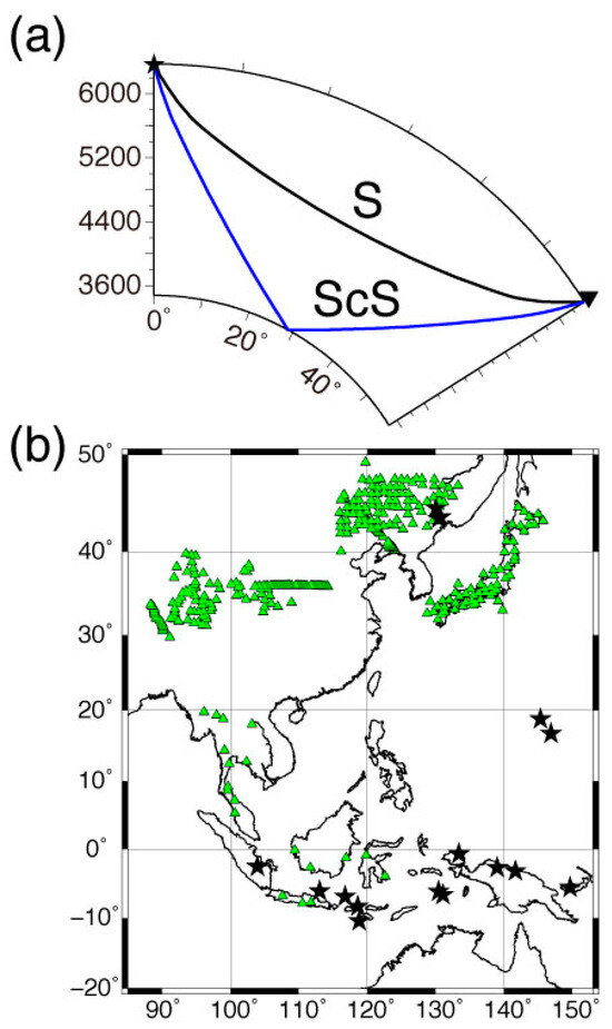
Figure 1.
(a) The ray paths of S and ScS phases. (b) Map of stations (green triangles) and epicenters (black stars) used in this study.

Table 1.
List of hypocenters and seismic network codes.
The primary data are the differential ScS–S travel-times. First, we applied the zero-phase band-pass filter with cut-off frequencies of 0.02 and 1.0 Hz on seismograms including S and ScS phases (Figure 2a). The resulting waveforms exhibited a typical predominant period of approximately 10 s. An S-wave pulse was sampled as a reference (marked by horizontal bars in Figure 2a). After an appropriate time shift with the maximum correlation coefficient between ScS and the sampled S-wave pulse, the sampled S-wave pulse was drawn on the ScS phase using a red segment, as shown in Figure 2a. Horizontal bars and red segments were drawn if the measurements were successful. The typical maximum correlation coefficient was 0.8–0.9. Although Stark and Forsyth [29] and their successors suggested that the attenuation factor should be applied on an S-wave pulse before taking the cross-correlation with later phases, such as ScS waveforms, we did not adopt this procedure. The differential attenuation parameter between S and ScS, Δt*ScS–S, is expected to be positive if we use a widely accepted Earth model, e.g., the Preliminary Reference Earth Model (PREM) [30]. However, this is not always the case, probably because the Q values in the region where the S waves pass are smaller than those for the ScS waves [31], or because of broadening of the S waves due to the slab diffraction [32]. Thus, we decided to avoid inferring additional unknown parameters, e.g., Δt*ScS–S, which might be significantly affected by ambient noises. If we assume that there is no small-scale lateral variation in the Q structure, only an offset of travel-time anomalies may exist.
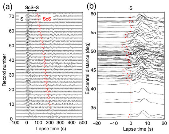
Figure 2.
(a) The record section of Event 8, including S and ScS phases. The sampled parts of the S phases are marked by horizontal bars; the red segments are S phases after relevant time shifts that succeeded and were used to measure the differential times of ScS–S. (b) The record section of Event 8, focused on S phases. The red dots indicate the timing of the manually picked arrival times. The horizontal axes are the lapse times from the theoretical S-wave arrivals.
We would like to point out that the auxiliary data represent the arrival times of the S and ScS phases. Figure 2b shows that the S arrivals were picked manually on the displacement seismograms after applying a causal filter with cut-off frequencies of 0.01–5 Hz or 0.03–5 Hz (Events 6, 12, 13, and 14). When we inferred the arrival times of the ScS phases, the observed differential travel times of ScS–S were added to the arrival times of the S phases, because the selection of the first motion of the ScS phases was quite challenging owing to the noise or contamination of S codas for many traces.
To calculate the reference travel times, the PREM was used, with a physical dispersion correction for the period of 10 s to adjust the predominant period of the observed waveforms. The observed travel times for S, ScS, and ScS–S were compared with the theoretical reference times. Ellipticity corrections [33] were applied to the S, ScS, and ScS–S travel-time residuals to obtain the differential travel-time residuals of ScS–S (ΔTScS–S), as well as the travel-time residuals of S (ΔTS) and ScS (ΔTScS).
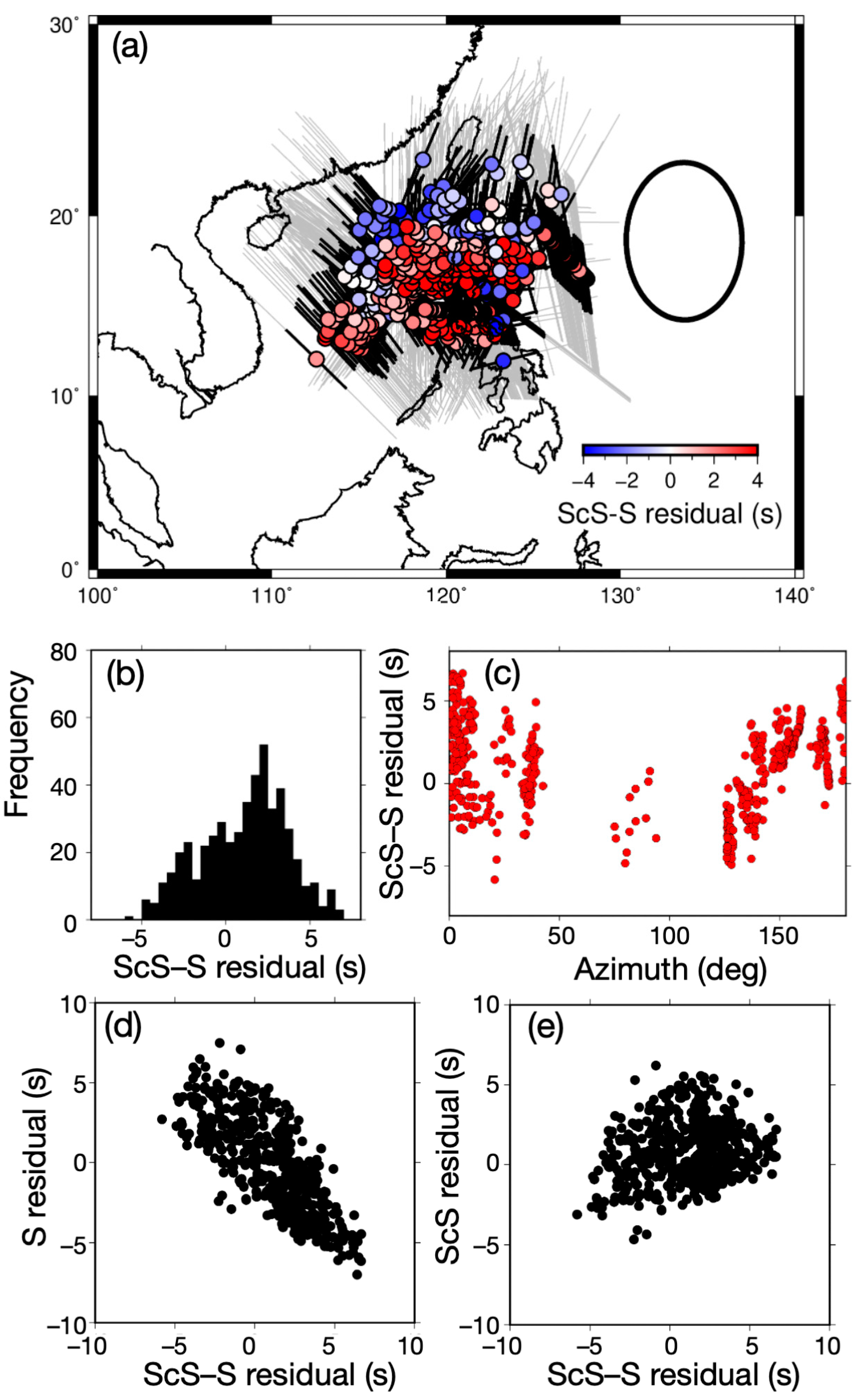
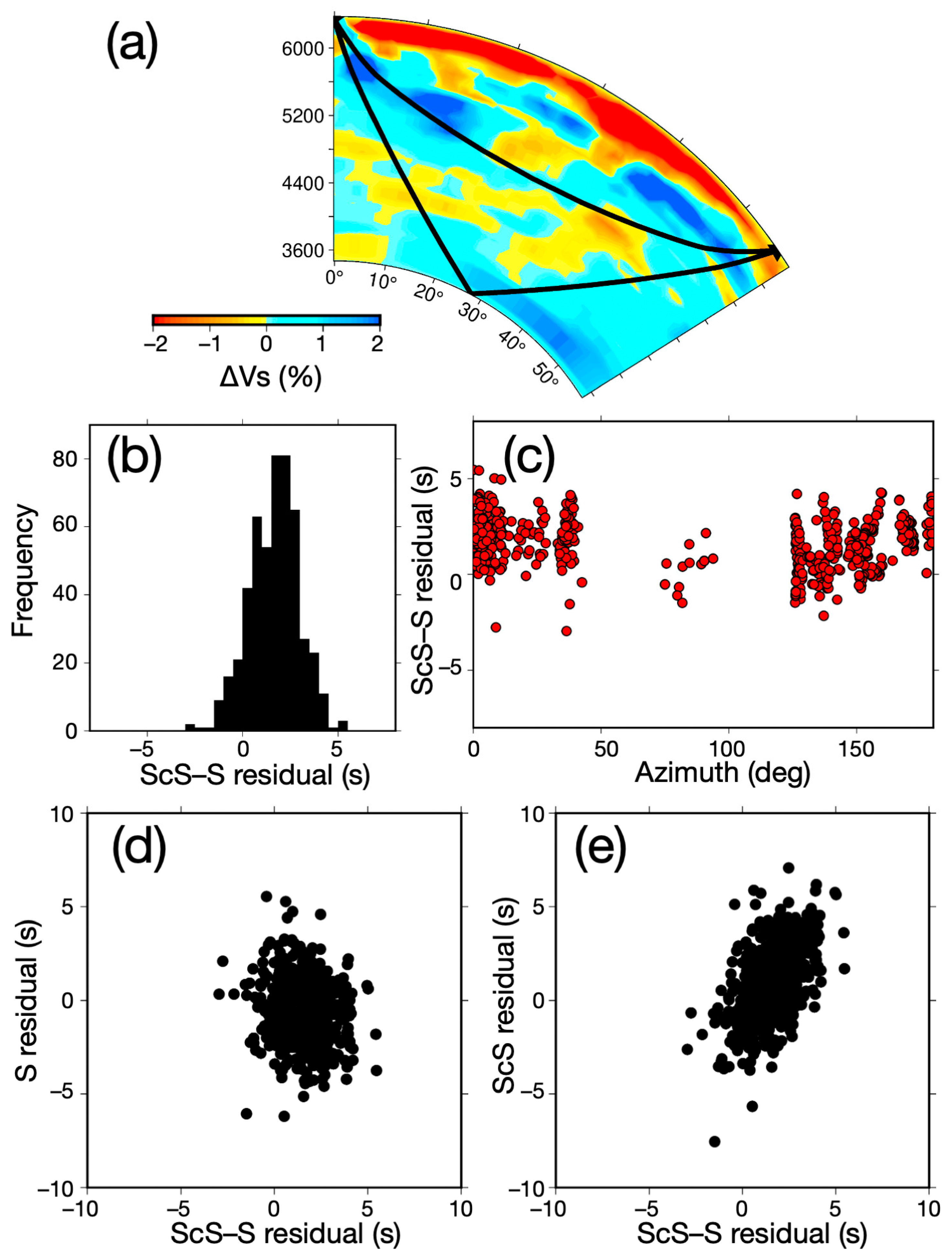
We obtained 501 measurements of the ΔTScS–S travel-time residuals with respect to the PREM. Approximately 5% of the measurements indicated that the cross-correlation coefficients between S and ScS waves were <0.7. However, we confirmed that the locations of the corresponding peaks between the two waveforms coincided well, and that the differential travel times were not very different from those observed at neighboring stations. The geographical distribution of ΔTScS–S plotted on the bounce points (reflection points) of the ScS phases, with the typical Fresnel zone of the ScS phase at the CMB for the period of 10 s, the histogram of ΔTScS–S, its azimuthal variation, and the correlation plots between ΔTScS–S and ΔTS and between ΔTScS–S and ΔTScS, are shown in Figure 3a–e, respectively. The ΔTScS–S residuals were widely scattered, with a standard deviation of 2.58 s (Figure 3b and Table 2). Although the ΔTScS–S residuals show clear azimuthal variations, ΔTScS–S is largely scattered within a narrow azimuthal range (Figure 3c) and strongly correlated with ΔTS rather than ΔTScS (Figure 3d,e and Table 2). This result indicates that ΔTScS–S should be corrected for mantle heterogeneity, particularly in the region where S waves are propagated, prior to discussing the lateral and azimuthal variations in the structure near the CMB, as well as azimuthal anisotropy.

Figure 3.
(a) The map of the ScS bounce points (reflection points) at the CMB, with color indicating the ScS–S residuals. The black and gray lines are the ScS ray paths passing through the lowermost 100 and 300 km in the mantle, respectively. The ellipse drawn on the right of the ScS bounce points expresses the Fresnel zone of the ScS phase passing in a north–south direction for the period of 10 s. (b) The histogram of the ScS–S residuals. (c) The azimuthal variation in the ScS–S residuals. The correlation plot of the ScS–S residuals with respect to the (d) S residuals and (e) ScS residuals.
Table 2.
Average and standard deviations of the corrected ΔTScS–S, and the correlation coefficients of ΔTScS–S vs. ΔTS and ΔTScS for non-corrected and corrected cases.
3. Analyses and Results
3.1. Three-Dimensional (3D) Mantle Correction
Representative 3D heterogeneity models of S16U6L8 [34], SB4L18 [35], S40RTS [36], SEMUCB-WM1 [37], and TX2019slab [38] for S-wave velocity, and of GAP-P4 [39] for P-wave velocity, with a conversion rate R = dlnVs/dlnVp, were selected. The reason for the addition of GAP-P4 will be discussed later. These models were used to correct the ScS–S differential travel times and the S and ScS travel times. The travel-time perturbation along each ray path was calculated using a simple ray-trace method with a one-dimensional velocity structure, as in the work of Tanaka [40], except for the typical layer thickness of 10 km.
Next, mantle heterogeneity correction was applied using existing 3D mantle models. To interpret our results, we first summarized the ΔTScS–S histograms after mantle corrections, following an example of S-wave velocity perturbations plotted on the cross-sections along a great circle path between an Indonesian event (Event 13) and a station in Northeastern China (NEA1: the northwestern corner of the NECESSArray) in Figure A1 (see Appendix A). As shown in the uppermost panels of Figure A1a–e, the fast-velocity region stretching from the hypocenter to the lower mantle is the subducting Australian Plate. It is clear that the older S16U6L8 and SB4L18 3D S-wave velocity models that were published before the early 2000s indicate that the spatial resolution in the lower mantle, particularly for the subducting slab, is not as high as that of the S40RTS, SEMUCB-WM, and TX2019slab models that were published in the 2010s. The ΔTScS–S scatters were significantly reduced after correction with S40RTS and TX2019slab, as shown in the center panels of Figure A1c,e and Table A1 (see Appendix A). However, the correlation between ΔTS and ΔTScS–S after correction using S40RTS, SEMUCB-WM, and TX2019slab was not significantly reduced as expected, as shown in the lowermost panels of Figure A1a–e and Table A1. This can be interpreted as the spatial resolution in the upper part of the lower mantle being insufficient and the S and ScS travel-time data contributing equally to the construction of these 3D mantle heterogeneity models.
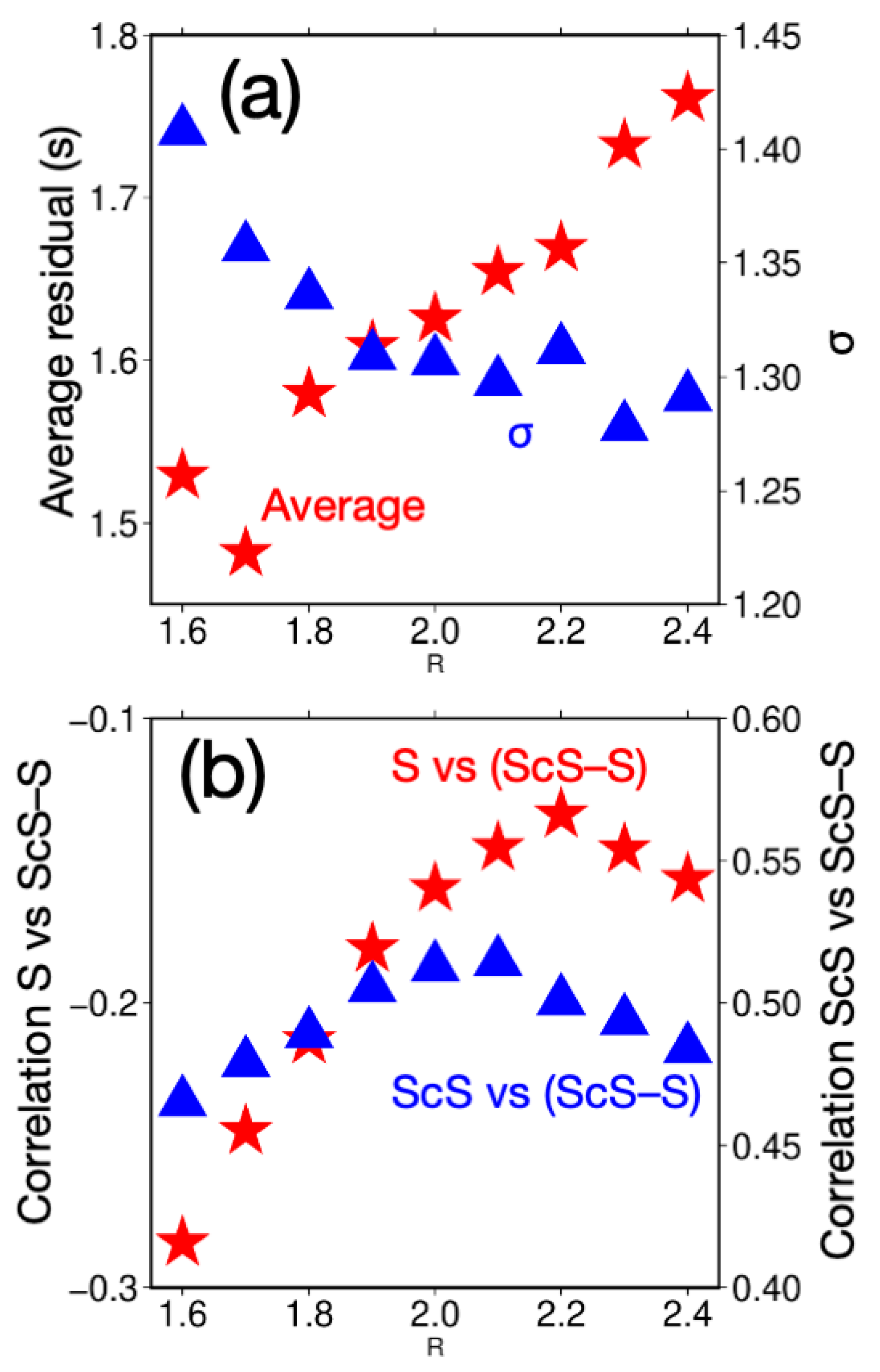
Based on the above example, we sought a model with a higher spatial resolution in the mantle, particularly where direct waves (such as S waves) are propagated. The P-wave velocity model has higher resolution in the upper part of the lower mantle, and GAP-P4 [39], which is characterized by a non-uniform grid size and aims to achieve high spatial resolution in the Western Pacific, was selected. To convert P-wave velocity perturbations into S-wave velocity perturbations, we determined the conversion rate (R = dlnVs/dlnVp) and its behavior with depth. The behavior of R in the mantle has not yet been determined [35,41,42,43,44]. Except for the theoretical study by Karato [41], in which the R value indicates a very small change of approximately 1.5 to 1.7, the inferred R value generally increases from 1.5 to 3 or 4 with increasing depth. However, when the depth-dependent R given by Bolton and Masters [43] was applied to the ScS–S residuals before the data collection was complete, the corrected residuals were more scattered than the original distribution. Therefore, we deduced that the constant R should be adopted. Bolton and Masters [43] indicated that the R value for the 2300–2900 km depth inferred from the data passing through fast regions was 1.8. Houser et al. [45] adopted a value of 1.7 in the upper mantle during their P-wave tomographic inversion under the constraint of the S-wave velocity model. Thus, we tested the R values from 1.6 to 2.4 with 0.1 intervals, as shown in Figure 4. The standard deviation σ of ΔTScS–S was not significantly reduced at R values ≥ 1.9, and the average of ΔTScS–S generally increased with increasing R values (Figure 4a). The absolute correlation between ΔTS and ΔTScS–S was minimal at R = 2.2, and that between ΔTScS and ΔTScS–S was maximal at R = 2.1 (Figure 4b). Considering the above results, we selected a value of 2.1 throughout the mantle in this study.
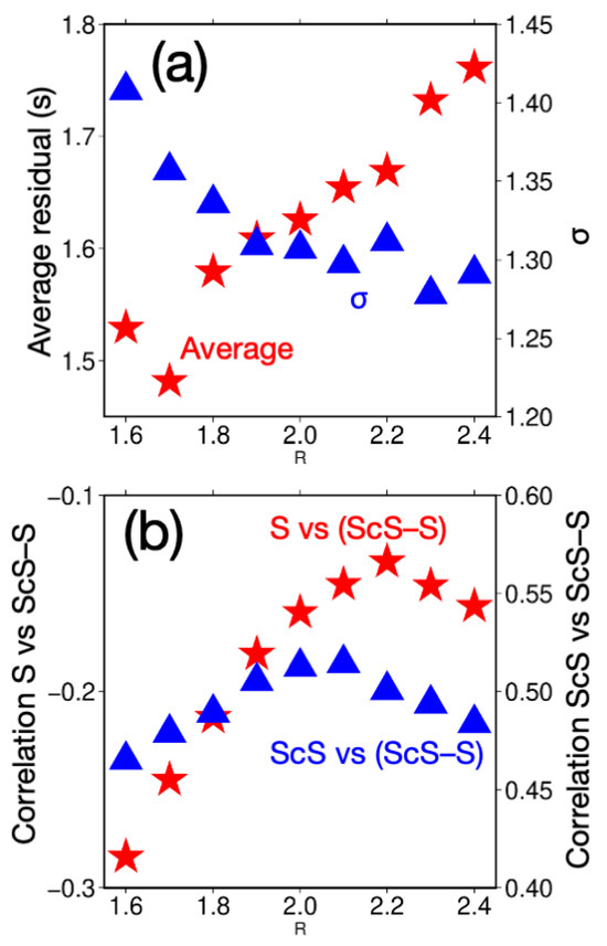
Figure 4.
(a) The averages (red stars) and standard deviations σ (blue triangles) of the ΔTScS–S residuals after correction using GAP-P4 with R. (b) The correlation coefficients between ΔTS and ΔTScS–S (red stars), and between ΔTScS and ΔTScS–S (blue triangles), as a function of R.
Figure 5a shows the S-wave velocity perturbations of the modified GAP-P4 with R = 2.1 on an example cross-section. This example clearly shows the existence of a subducting slab, which is the most important for ΔTScS–S correction. As shown in Figure 5b and Figure A1, and in Table 2 and Table A1, the scattering of the ΔTScS–S residuals corrected with the modified GAP-P4 of R = 2.1 was the least among the corrected residuals. The magnitude and behavior of the azimuthal variation in ΔTScS–S became small and simple, respectively (Figure 5c). The correlation coefficient between ΔTS and ΔTScS–S was significantly reduced to <0.2 by the correction (Figure 5d and Table 2), whereas that between ΔTScS and ΔTScS–S exceeded 0.5 (Figure 5e and Table 2). Thus, we suggest that the corrected ΔTScS–S residuals are primarily influenced by the structure of the lower mantle, where only ScS phases traverse, probably because the modified GAP-P4 does not fully represent the heterogeneous and possibly anisotropic structures of this region.
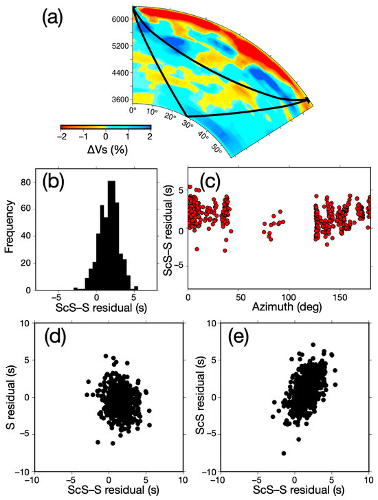
Figure 5.
(a) S-wave velocity perturbations of the modified GAP-P4 with R = 2.1 projected on the cross-section between an Indonesian event (Event 13) and a station in Northeastern China (Station NEA1, located at the northwestern corner of NECESSArray), and ray paths of S and ScS phases. (b) The histogram of ΔTScS–S. (c) The azimuthal variation in ΔTScS–S. (d) The correlation plot between ΔTScS–S and ΔTS, and (e) between ΔTScS–S and ΔTScS.
3.2. Correction for Local Heterogeneity
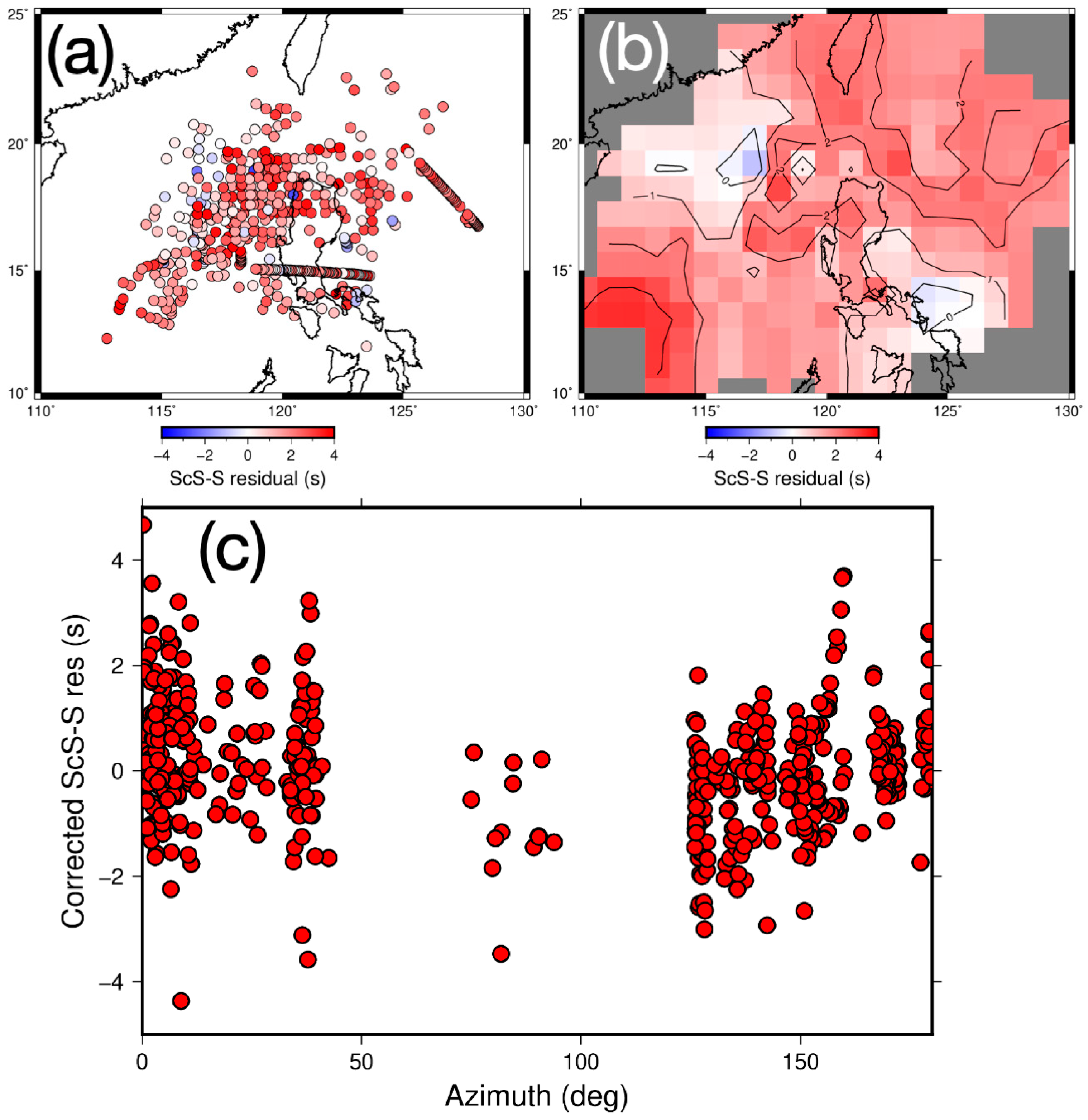
Although the correlation coefficient between ΔTScS–S and ΔTScS moderately increased, and the standard deviations of the ΔTScS–S residuals were significantly reduced after 3D mantle correction, the average of the residuals was 1.65 s, which is greater than the non-corrected value (Table 2). This is probably because the corrections with GAP-P4 for ScS travel times are opposite, and the spatial resolution of GAP-P4 in the lowermost mantle is insufficient. To reduce the average residual and effects of the local heterogeneity that were not fully represented by the modified GAP-P4, we obtained the weighted averages of the residuals at every 1° grid, with a search radius of 4°, using the “nearneighbor” command of Genetic Mapping Tools ver.6 [46]. The search radius of 4° was selected while referencing the Fresnel zone size, as shown in Figure 2. Figure 6a,b show the maps for the ΔTScS–S residuals corrected for mantle heterogeneity with the modified GAP-P4 discussed in the previous section at the ScS bounce points (reflection points) at the CMB and the smoothed one, respectively. The ΔTScS–S residuals were further corrected by subtracting the interpolated residuals from the smoothed residuals shown in Figure 6b to obtain ΔTScS–S as a function of the propagation azimuth (Figure 6c).

Figure 6.
(a) Geographical distribution of the ScS bounce points (reflection points) and the corrected ΔTScS–S presented by a color scale. (b) The map of the smoothed ΔTScS–S. (c) The azimuthal variation in the corrected ΔTScS–S residuals.
3.3. Attempt at Anisotropic Parameter Estimation
To model the azimuthal variation in the ΔTScS–S residuals, it was assumed that ΔTScS–S after many corrections can be expressed as follows [47,48]:
where A, B, C, and D are the amplitudes of the azimuthal terms, E is the average of the residuals, and θ is the ray azimuth of the ScS phase at the CMB bounce point. The A, B, C, and D parameters can be estimated using the least-squares method; then, they are converted to a, b, ϕ, and, ψ, as expressed below [24]:
where ϕ and ψ are the azimuthal offsets of the 2θ and 4θ terms, respectively. The results of the least-squares inference are summarized in Table A2 (see Appendix A). Furthermore, because the ΔTScS–S scatter was very large and we wanted to directly obtain the anisotropic parameters and their uncertainties in Equation (2), we applied Bayesian inference using PyMC ver.5 [49,50], in which a statistical model is defined as follows:
where N is a normal distribution. For prior distributions, normal distributions are used for a, b, ϕ, ψ, and E, and a half-normal distribution ε is assumed for the noise term σ. A No-U-Turn Sampler (NUTS) [51] was used for sampling. We increased the sampling number from 2000 to 40,000 in six chains until the message “The effective sample size per chain is smaller than 100 for some parameters” no longer appeared. However, the NUTS still returned several divergences, suggesting that parameterization using Equations (2) and (3) was not appropriate, particularly for the estimation of ψ. In the a posteriori distribution of ψ, two peaks were found, probably due to the very small values of b, as shown in Figure A2 and Table A3 (see Appendix A).
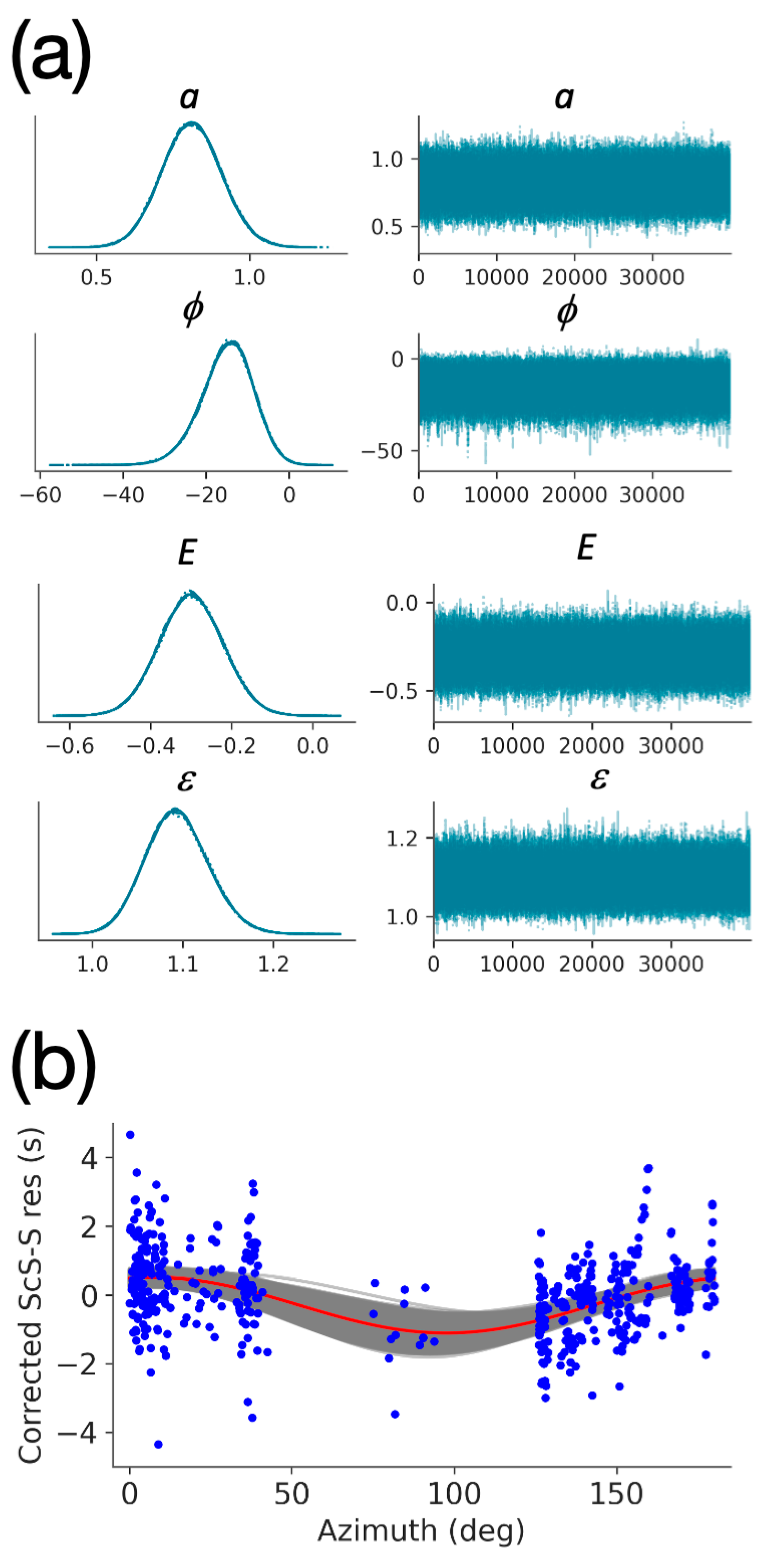
Thus, we omitted the 4θ terms to obtain a, ϕ, E, and ε, as shown in Figure 7a and Table 3. The average azimuthal variation model, with model uncertainties resampled from the posterior distribution of each parameter, is shown in Figure 7b. Although the data scatter was very large for every data cluster, the model uncertainties were small at azimuths of 0–50° and 120–150°, where the data were concentrated, whereas the uncertainties were large at azimuths of 70–110°, where the data were sparsely distributed. The peak-to-peak amplitude of ΔTScS–S was approximately 1.6 s, and the largest and smallest ΔTScS–S values appeared at azimuths of 7.5° and 97.5°, respectively. Furthermore, the sums of the squared residuals for the models of the 2θ term and 2θ and 4θ terms were 592.6 and 593.06, respectively, and the Akaike information criterion for unknown uncertainties of measurements [52] was 6403.28 and 6408.06, respectively, which supports the 2θ term model.
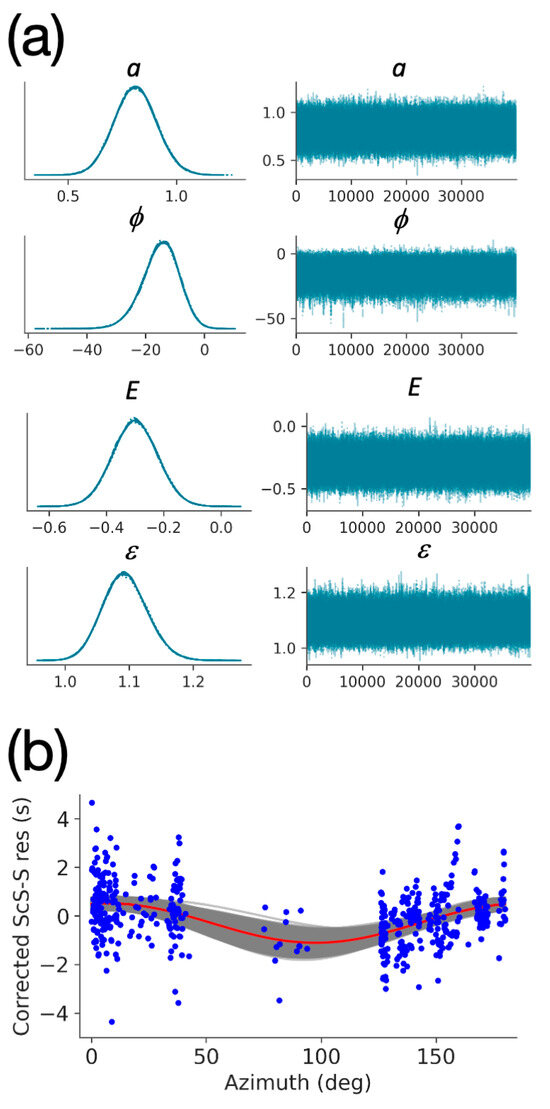
Figure 7.
(a) The posterior distributions for the estimated parameters of a, ϕ, E, and ε. (b) The estimated model of the ΔTScS–S azimuthal variation (the red line) and uncertainties (gray lines) with data (blue dots).
Table 3.
The anisotropic parameters estimated with a Bayesian inference.
4. Discussion
4.1. Possible Interpretation of ScS–S Residuals Except for Azimuthal Anisotropy
As shown in the previous sections, the differential travel-time residuals ΔTScS–S have large scattering even within a narrow azimuth range. Ambient noise can result in scatters as large as 1 s [40]. Small-scale unmodeled subducting slabs can affect the travel times and waveforms of the S waves, which may also result in such scattered residuals. On the other hand, small-scale heterogeneity that exists along the ScS phases, e.g., heterogeneities in and above the D″ region, can be considered. For example, small-scale lateral variations and/or strong changes in the topography of the D″ boundary can also cause the observed signal in the ScS–S times. Furthermore, the most important data shown in Figure 7b to recognize the existence of the apparent azimuthal variation and to distinguish the 2θ and 4θ contributions are the residuals ΔTScS–S at azimuths around 90°, which are obtained by the combination of the Marianan events and the Thai stations. Figure A3 (see Appendix A) shows the S-wave velocity perturbation of the modified GAP-P4 on the vertical cross-section between Marina and Thailand, indicating that the subducting slab reaches approximately 900 km depth, and the anomalies of both the S and ScS travel times due to the slab would be almost the same. However, if undetected structural anomalies along ScS phases exist, e.g., a fast velocity extending downward, the pattern of the azimuthal variation of ΔTScS–S can be changed after the correction. Furthermore, to fully address this issue, filling the current azimuthal gaps in ΔTScS–S is also important.
4.2. Speculation for Azimuthal Anisotropy
In this section, we would like to try to estimate the possible anisotropy parameters. Auxiliary information is required to assess the magnitude of the anisotropy at the base of the mantle. The thickness of the D″ discontinuity beneath the Western Pacific, including the Philippines, is estimated to be 240–350 km with large scattering [53,54]. Considering the amplitude of the 2θ contribution in the ScS–S residuals corrected by the modified GAP-P4—that is, 1.6 s peak-to-peak (Figure 7b and Table 3)—combined with the assumptions of the thickness of 300 km, the incident angle of 45°, and the constant shear-wave velocity in the D″ region as 7.24 km/s taken from the PREM, for simplicity, the magnitude of anisotropy was roughly estimated to be approximately 1.4%.
Figure 8 presents a summary of this study. The direction of the minimum ScS–S residuals corresponding to the fastest SH velocity at the CMB was east-southeast–west-northwest (N97.5° E–N82.5° W). Interestingly, this direction is almost parallel to the direction of the Philippines Sea Plate (PHS) and Sunda Block [55], which suggests that surface plate motion may be related to the flow at the base of the mantle, and vice versa. Furthermore, the instantaneous mantle flow converted by the 3D mantle model derived by Yoshida [56] and Yoshida [57] indicates that the direction of mantle flow at the CMB is oriented from the Philippines to the Caroline hotspot, which is consistent with the direction of the minimum ScS–S residuals.
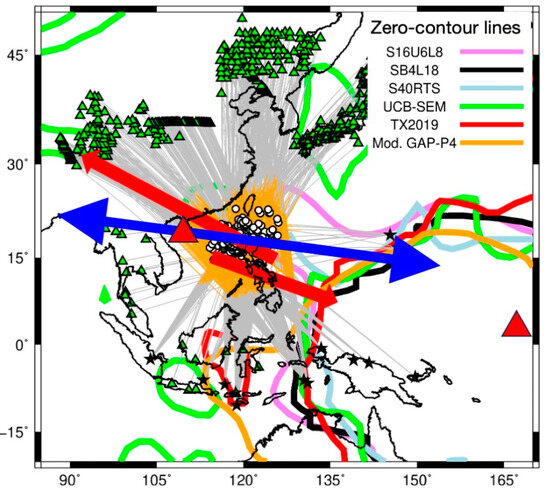
Figure 8.
Geographical distribution of the ScS bounce points, the ScS ray paths (the gray lines) and those passing through the lowermost 300 km in the mantle (the orange lines), the sources (the black stars) and receivers (the green triangles), and the zero-contour lines of perturbations in the seismic wave velocity at the base of the mantle, taken from S16U6L8, SB4L18, S40RTS, SEMUCB-WM, and the modified GAP-P4. The directions of the absolute plate motions of the Philippines Sea (PHS) plate, the Sunda Block (red arrows), and the fast S-wave velocity (blue arrow) are superimposed. The Caroline hotspot is represented by the red triangle.
Figure 8 shows the zero-contour lines of the S-wave velocity perturbation at the CMB, which represent the edges of the Pacific LLVP. As mantle flow may be influenced by LLVPs and mantle plumes [15,16,19,58,59,60,61], it is worthwhile to briefly compare our observation with the theoretical predictions of the azimuthal variations in S-wave velocity for deformed post-perovskite, which are believed to be a plausible candidate for the D″ anisotropy mechanism. Creasy et al. [10] constructed a library of the elastic constants undergoing possible deformation mechanisms using viscoplastic self-consistent modeling [62], from which we focused on three slip systems for post-perovskite (Ppv1: (010) <100> dominant slip system, Ppv2: (001) <100>, and Ppv3: {011} <0–11> + (010) <100>), where a starting single-crystal elastic tensor at 125 GPa and 2500 K [63] was used along with three deformation scenarios of (1) simple shear, (2) pure shear, and (3) extension. The SH velocities for the elastic tensors modeled with the combination of the slip systems and deformation scenarios were calculated with the MSAT toolkit [64], from which the “MS-rot3” function was applied, which rotates an elastic tensor around three axes. The variation in the velocity with azimuth and incident angles was determined by rotating the elastic tensor about the vertical x3 and horizontal x2 axes [48], respectively, and then was calculated using the rotated elastic tensor. As the ScS phases were primarily analyzed at shorter distances of 45–60° in this study, the incident angles were fixed at 45° for simplicity. To compare our observations, we calculated the VSH for nine combinations of three slip systems (Ppv1, Ppv2, and Ppv3) and three deformation scenarios: (1) simple shear, (2) pure shear, and (3) extended. Figure A4 (see Appendix A) shows the azimuthal variation in VSH for incident angles of 45 and 0°, which correspond to the case of the diffracted S or ScS phases at greater distances, for comparison, in the azimuth range from 0 to 180°. The VSH at incident angles of 0 and 45° showed a 4θ dependence for every combination of slip systems and deformation scenarios. In the cases considered, we did not find a 2θ variation that was consistent with our observations. As the observed 2θ variation in ΔTScS–S is the result of many correction steps and retains a large data scatter, observations as well as tests of the other elastic tensors should be improved upon.
5. Conclusions
The ScS–S differential travel-time residuals with various ray directions were analyzed to investigate the possibility of seismic azimuthal anisotropy in the lowermost mantle beneath the Philippines after appropriate corrections. In this study, approximately 500 ScS–S differential travel-time residuals were corrected by an appropriate 3D mantle heterogeneity model (P-wave velocity GAP-P4 model with a Vp-to-Vs conversion ratio R (=dlnVs/dlnVp) = 2.1), correlated with those of ScS rather than with those of the S phase, and after local heterogeneity corrections, our analysis indicated the azimuthal variation, in which 2θ contributions may be significant. Although many corrections were applied, the data scatter was large, and many other possible interpretations remained, this observation may be interpreted as a manifestation of azimuthal anisotropy in the lowermost mantle. If we accept this hypothesis, the fastest direction of S-wave velocity in the lowermost mantle beneath the Philippines was east-southeast–west-northwest (N97.5° E–N82.5° W), and the magnitude of anisotropy was approximately 1.4% if a D” thickness of 300 km is assumed.
Funding
This research received no external funding.
Data Availability Statement
The raw data supporting the conclusions of this article will be made available by the author on request.
Acknowledgments
The comments by the three reviewers improved this manuscript.
Conflicts of Interest
The author declares no conflicts of interest.
Appendix A
Figure A1: The cross-sections of 3D mantle S-wave models between an Indonesian event (Event 13) and a station in Northeastern China (Station NEA1, which is located at the northwestern corner of NECESSArray), the histograms of the corrected ΔTScS–S, and the correlation plots between the corrected ΔTS and ΔTScS–S, and between the corrected ΔTScS–S and ΔTScS–S, for the 3D S-wave mantle models considered in this study. Figure A2: The results of the Bayesian inference for anisotropic parameters of Equation (3). Figure A3: S-wave velocity perturbations of the modified GAP-P4 with R = 2.1 projected on the cross-section between a Marianan event (Event 15) and station in Thailand (CHTO). Figure A4: Azimuthal variations in SH velocities for various elastic tensors. Table A1: Average and standard deviations of the corrected ΔTScS–S, and the correlation coefficients of ΔTScS–S vs. ΔTS and ΔTScS, for the 3D S-wave mantle models considered in this study. Table A2: The anisotropic parameters estimated using least-squares inference. Table A3: All of the anisotropic parameters of Equations (2) and (3), estimated with Bayesian inference.
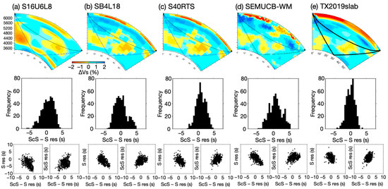
Figure A1.
The cross-sections of 3D mantle S-wave models of (a) S16U6L8, (b) SB4L18, (c) S40RTS, (d) SEMUCB-WM, and (e) TX2019slab between an Indonesian event (Event 13) and a station in Northeastern China (Station NEA1, which is located at the northwestern corner of NECESSArray) (top panel), the histograms of the corrected ΔTScS–S (middle panel), and the correlation plots between the corrected ΔTS versus ΔTScS–S (bottom left) and the corrected ΔTScS–S versus ΔTScS–S (bottom right) for the 3D S-wave mantle models considered in this study.
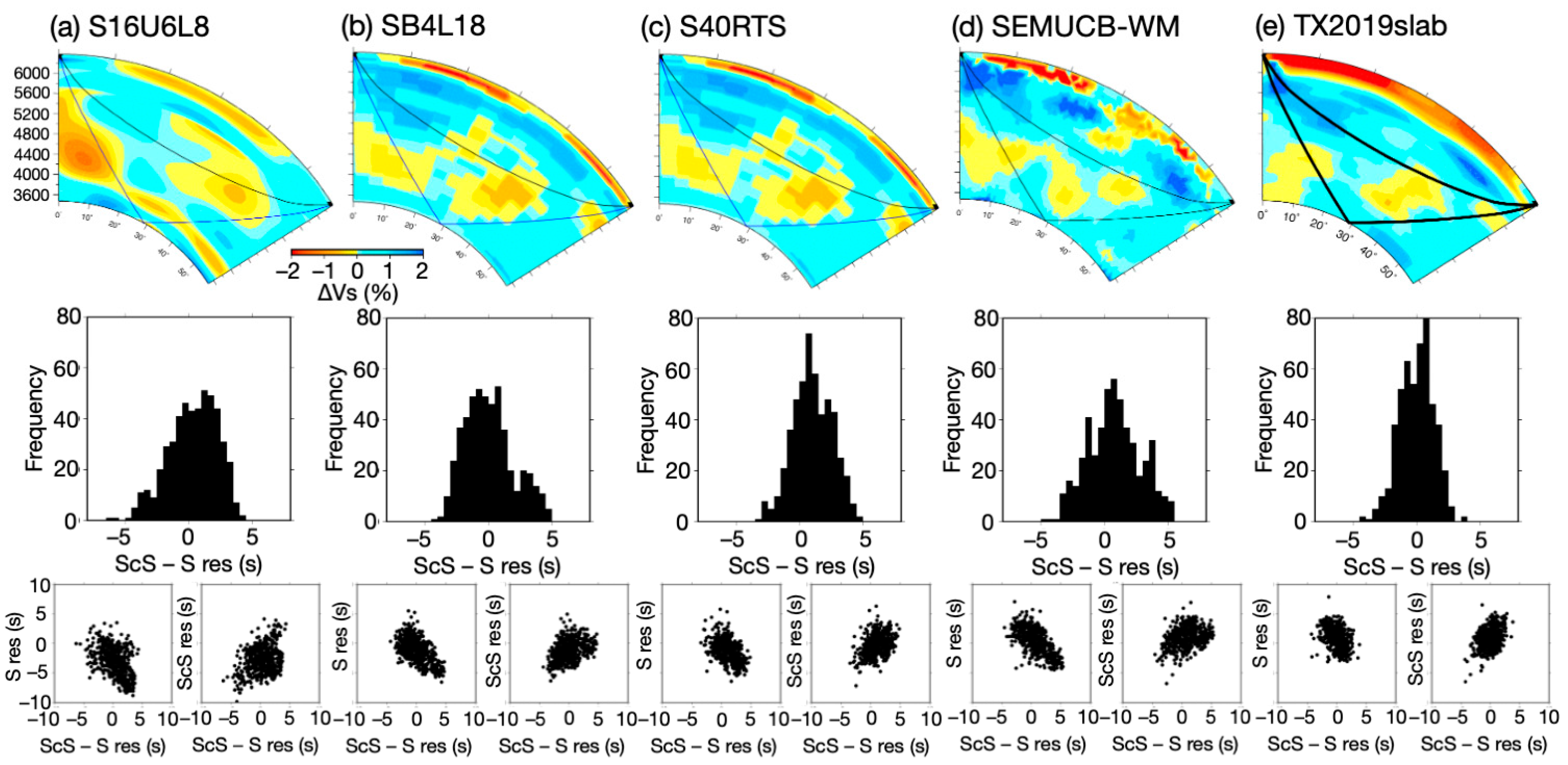
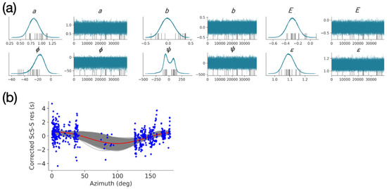
Figure A2.
The results of the Bayesian inference for full anisotropic parameters of Equation (3): (a) The posterior distributions for the estimated parameters of a, b, ϕ, ψ, E, and ε. (b) The estimated model of the ΔTScS–S azimuthal variation (the red line) and uncertainties (gray lines) with data (blue dots).
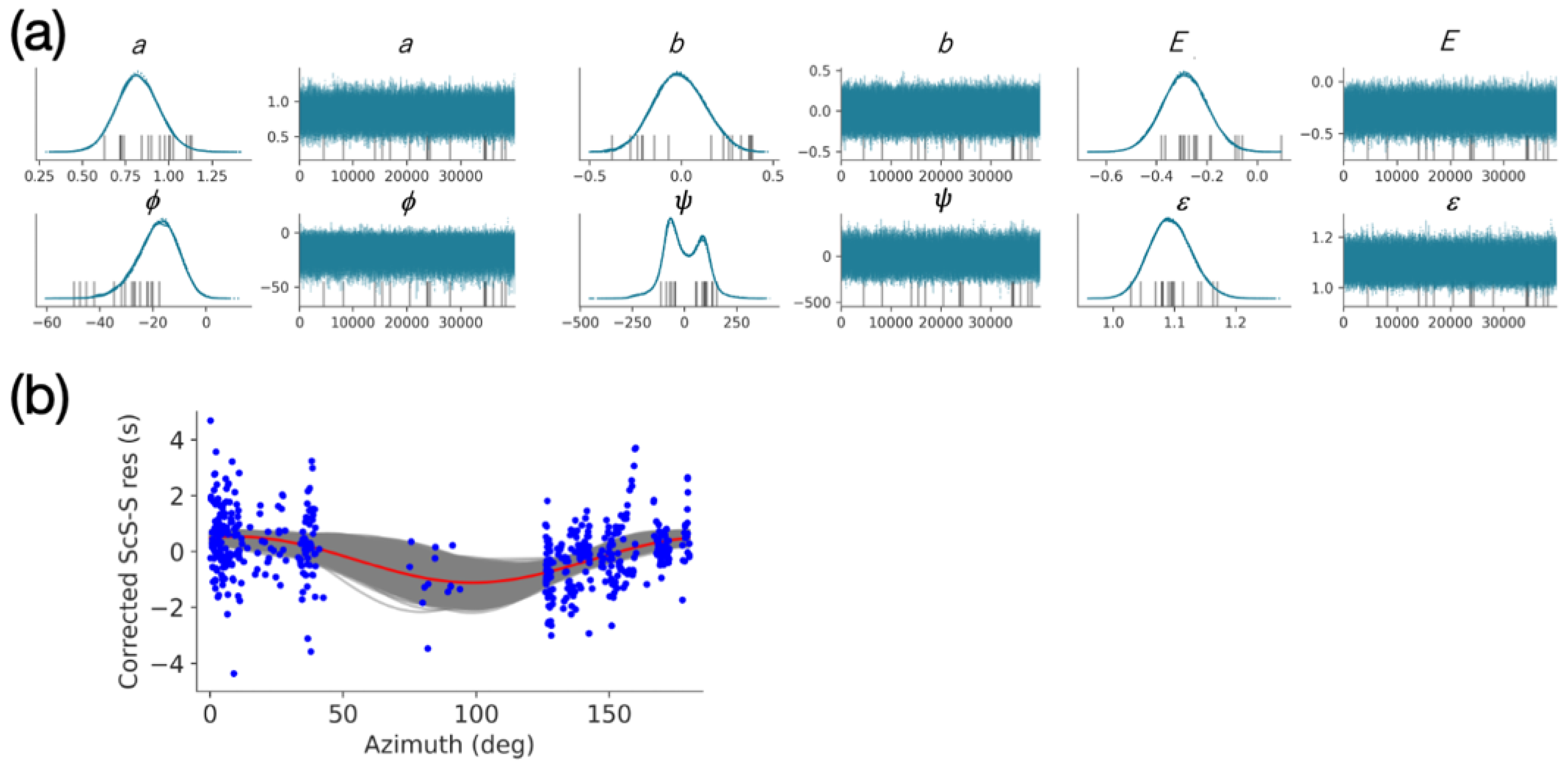
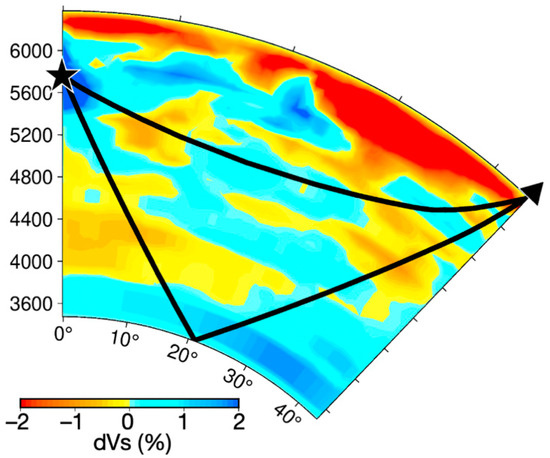
Figure A3.
S-wave velocity perturbations of the modified GAP-P4 with R = 2.1 projected on the cross-section between a Marianan event (Event 15; black star) and a station in Thailand (CHTO; black triangle).
Figure A3.
S-wave velocity perturbations of the modified GAP-P4 with R = 2.1 projected on the cross-section between a Marianan event (Event 15; black star) and a station in Thailand (CHTO; black triangle).
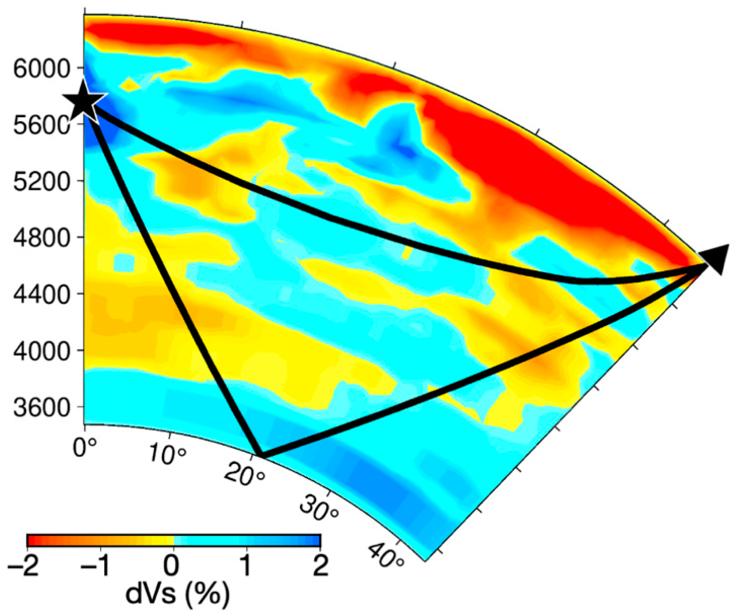
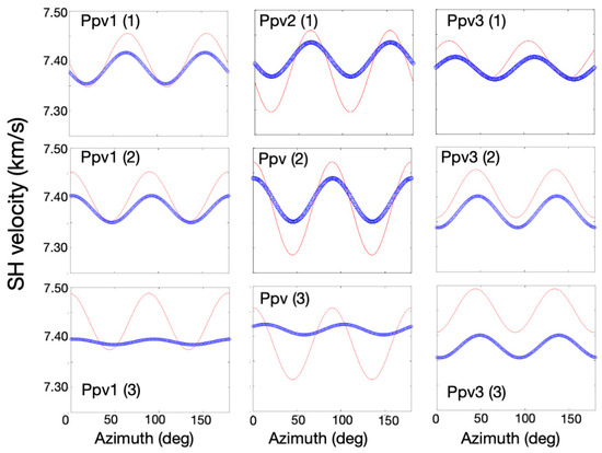
Figure A4.
Azimuthal variations in SH velocities for various elastic tensors with slip systems and deformation scenarios. The blue circles and red lines show the case of the incident angles of 45° and 0°, respectively, with respect to the x1-x2 plane.
Figure A4.
Azimuthal variations in SH velocities for various elastic tensors with slip systems and deformation scenarios. The blue circles and red lines show the case of the incident angles of 45° and 0°, respectively, with respect to the x1-x2 plane.
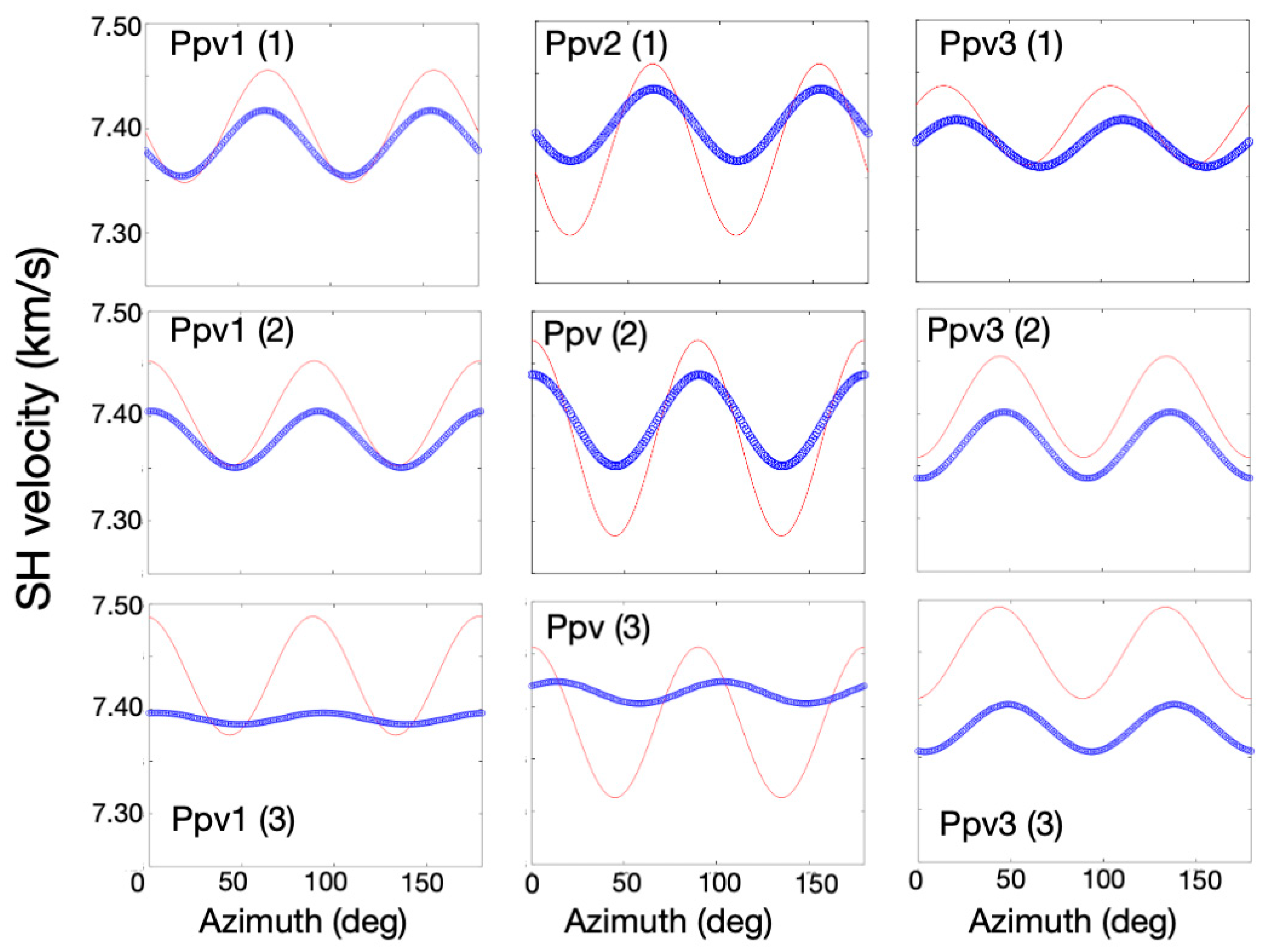
Table A1.
Average and standard deviations of the corrected ΔTScS–S, along with the correlation coefficients of ΔTScS–S vs. ΔTS and ΔTScS for various 3D S-wave mantle models.
Table A1.
Average and standard deviations of the corrected ΔTScS–S, along with the correlation coefficients of ΔTScS–S vs. ΔTS and ΔTScS for various 3D S-wave mantle models.
| Model for Correction | Average (s) | Standard Deviation (s) | Correlation Coefficient of ΔTScS–S vs. ΔTS | vs. ΔTScS |
|---|---|---|---|---|
| S16U6L8 | 0.34 | 1.92 | −0.49 | 0.31 |
| SB4L18 | 0.03 | 1.90 | −0.59 | 0.38 |
| S40RTS | 1.01 | 1.54 | −0.42 | 0.43 |
| UCB-SEM-WM | 0.78 | 2.03 | –0.67 | 0.30 |
| TX2019slab | 0.00 | 1.33 | −0.38 | 0.38 |
Table A2.
The anisotropic parameters estimated with the least-squares inference.
Table A2.
The anisotropic parameters estimated with the least-squares inference.
| Parameters | Inferred Value | Standard Deviation |
|---|---|---|
| a | 0.84 | 0.13 |
| ϕ | −19.84 | 13.08 |
| b | 0.13 | 0.10 |
| ψ | 108.23 | 22.67 |
| E | −0.28 | 0.09 |
Table A3.
The anisotropic parameters of Equation (2) estimated with a Bayesian inference.
Table A3.
The anisotropic parameters of Equation (2) estimated with a Bayesian inference.
| Parameters | Average | Standard Deviation |
|---|---|---|
| a | 0.82 | 0.12 |
| ϕ | −18.16 | 7.69 |
| b | −0.01 | 0.14 |
| ψ | −0.63 | 91.15 |
| E | −0.30 | 0.09 |
| ε | 1.09 | 0.04 |
References
- McNamara, A.K. A review of large low shear velocity provinces and ultra low velocity zones. Tectonophysics 2019, 760, 199–220. [Google Scholar] [CrossRef]
- Dziewonski, A.M. Mapping the lower mantle: Determination of lateral heterogeneity in P velocity up to degree and order 6. J. Geophys. Res. 1984, 89, 5929–5952. [Google Scholar] [CrossRef]
- Tanimoto, T. Long-wavelength S-wave velocity structure throughout the mantle. Geophys. J. Int. 1990, 100, 327–336. [Google Scholar] [CrossRef]
- Fichtner, A.; Kennett, B.L.; Tsai, V.C.; Thurber, C.H.; Rodgers, A.J.; Tape, C.; Rawlinson, N.; Borcherdt, R.D.; Lebedev, S.; Priestley, K.; et al. Seismic Tomography 2024. Bull. Seismol. Soc. Am. 2024, 114, 1185–1213. [Google Scholar] [CrossRef]
- Garnero, E.J.; McNamara, A.K.; Shim, S.H. Continent-sized anomalous zones with low seismic velocity at the base of Earth’s mantle. Nat. Geosci. 2016, 9, 481–489. [Google Scholar] [CrossRef]
- Suetsugu, D.; Isse, T.; Tanaka, S.; Obayashi, M.; Shiobara, H.; Sugioka, H.; Kanazawa, T.; Fukao, Y.; Barruol, G.; Reymond, D. South Pacific mantle plumes imaged by seismic observation on islands and seafloor. Geochem. Geophys. Geosyst. 2009, 10, Q11014. [Google Scholar] [CrossRef]
- Li, J.; Zhang, B.; Sun, D.; Tian, D.; Yao, J. Detailed 3D Structures of the Western Edge of the Pacific Large Low Velocity Province. J. Geophys. Res. Solid Earth 2024, 129, e2023JB028032. [Google Scholar] [CrossRef]
- Yu, S.L.; Garnero, E.J. Ultralow velocity zone locations: A global assessment. Geochem. Geophys. Geosyst. 2018, 19, 396–414. [Google Scholar] [CrossRef]
- Wolf, J.; Long, M.D.; Li, M.; Garnero, E. Global Compilation of Deep Mantle Anisotropy Observations and Possible Correlation With Low Velocity Provinces. Geochem. Geophys. Geosyst. 2023, 24, e2023GC011070. [Google Scholar] [CrossRef]
- Creasy, N.; Miyagi, L.; Long, M.D. A library of elastic tensors for lowermost mantle seismic anisotropy studies and comparison with seismic observations. Geochem. Geophys. Geosyst. 2020, 21, e2019GC008883. [Google Scholar] [CrossRef]
- Romanowicz, B.; Wenk, H.R. Anisotropy in the deep Earth. Phys. Earth Planet. Inter. 2017, 269, 58–90. [Google Scholar] [CrossRef]
- Nowacki, A.; Wookey, J.; Kendall, J.M. New advances in using seismic anisotropy, mineral physics and geodynamics to understand deformation in the lowermost mantle. J. Geodyn. 2011, 52, 205–228. [Google Scholar] [CrossRef]
- Thomas, C.; Wookey, J.; Simpson, M. D″ anisotropy beneath Southeast Asia. Geophys. Res. Lett. 2007, 34, L04301. [Google Scholar] [CrossRef]
- Roy, S.K.; Kumar, M.R.; Srinagesh, D. Upper and lower mantle anisotropy inferred from comprehensive SKS and SKKS splitting measurements from India. Earth Planet. Sci. Lett. 2014, 392, 192–306. [Google Scholar] [CrossRef]
- Wolf, J.; Long, M.D. Slab-driven flow at the base of the mantle beneath the northeastern Pacific Ocean. Earth Planet. Sci. Lett. 2022, 594, 117758. [Google Scholar] [CrossRef]
- Asplet, J.; Wookey, J.; Kendall, M. A potential post-perovskite province in D″ beneath the Eastern Pacific: Evidence from new analysis of discrepant SKS–SKKS shear-wave splitting. Geophys. J. Int. 2020, 221, 2075–2090. [Google Scholar] [CrossRef]
- Wookey, J.; Kendall, J.M.; Rümpker, G. Lowermost mantle anisotropy beneath the north Pacific from differntial S–ScS splitting. Geophys. J. Int. 2005, 161, 829–838. [Google Scholar] [CrossRef]
- Wolf, J.; Long, M.D.; Leng, K.; Nissen-Meyer, T. Constraining deep mantle anisotropy with shear wave splitting measurements: Challenges and new measurement strategies. Geophys. J. Int. 2022, 230, 507–527. [Google Scholar] [CrossRef]
- Wolf, J.; Long, M.D. Lowermost mantle structure beneath the central Pacific ocean: Ultralow velocity zones and seismic anisotropy. Geochem. Geophys. Geosyst. 2023, 24, e2022GC010853. [Google Scholar] [CrossRef]
- Ishise, M.; Kawakatsu, H.; Morishige, M.; Shiomi, K. Radial and azimuthal anisotropy tomography of the NE Japan subduction zone: Impllications for the Pacific slab and mantle wedge dynamics. Geophys. Res. Lett. 2018, 45, 3923–3931. [Google Scholar] [CrossRef]
- Liu, X.; Zhao, D. P-wave anisotropy, mantle wedge flow and olivine fabrics beneath Japan. Geophys. J. Int. 2017, 210, 1410–1431. [Google Scholar] [CrossRef]
- Liu, X.; Zhao, D. Seismic velocity azimuthal anisotropy of the Japan subduction zone: Constraints from P and S wave traveltimes. J. Geophys. Res. Solid Earth 2016, 121, 5086–5115. [Google Scholar] [CrossRef]
- Fan, J.; Zhao, D.; Li, C.; Liu, L.; Dong, D. Remnants of shifting early Cenozoic Pacific lower mantle flow imaged beneath the Philippine Sea Plate. Nat. Geosci. 2024, 17, 347–352. [Google Scholar] [CrossRef]
- Kuo, B.-Y.; Forsyth, D.W.; Wysession, M.E. Lateral heterogeneity and azimuthal anisotropy in the north Atlantic determined from SS–S differential travel times. J. Geophys. Res. 1987, 92, 6421–6436. [Google Scholar] [CrossRef]
- Tang, Y.; Obayashi, M.; Niu, F.; Grand, S.P.; Chen, Y.J.; Kawakatsu, H.; Tanaka, S.; Ning, J.; Ni, J.F. Changbaishan volcanism in northeast China linked to subduction-induced mantle upwelling. Nat. Geosci. 2014, 7, 470–475. [Google Scholar] [CrossRef]
- Ohtaki, T.; Suetsugu, D.; Kanjo, K.; Purwana, I. Evidence for a thick mantle transition zone beneath the Philippine Sea from multiple-ScS waves recorded by JISNET. Geophys. Res. Lett. 2002, 29, 24-1–24-4. [Google Scholar] [CrossRef]
- Okada, Y.; Kasahara, K.; Hori, S.; Obara, K.; Sekiguchi, S.; Fujiwara, H.; Yamamoto, A. Recent progress of seismic observation networks in Japan –Hi-net, F-net, K-NET and KiK-net–. Earth Planets Space 2004, 56, xv–xxviii. [Google Scholar] [CrossRef]
- Engdahl, E.R.; van der Hilst, R.D.; Buland, R.P. Global teleseismic earthquake relocation with improved travel times and procedures for depth determination. Bull. Seism. Soc. Am. 1998, 88, 722–743. [Google Scholar] [CrossRef]
- Stark, M.; Forsyth, D.W. The geoid, small-scale convection, and differential travel time anomalies of shear waves in the central Indian ocean. J. Geophys. Res. 1983, 88, 2273–2288. [Google Scholar] [CrossRef]
- Dziewonski, A.M.; Anderson, D.L. Preliminary reference Earth model. Phys. Earth Planet. Inter. 1981, 25, 297–356. [Google Scholar] [CrossRef]
- Tanaka, S.; Hamaguchi, H. Heterogeneity in the lower mantle beneath Africa, as revealed from S and ScS phases. Tetonophysics 1992, 209, 213–222. [Google Scholar] [CrossRef]
- Cormier, V.F. Slab diffraction of S waves. J. Geophys. Res. 1989, 94, 3006–3024. [Google Scholar] [CrossRef]
- Kennett, B.L.N.; Gudmundsson, O. Ellipticity corrections for seismic phases. Geophys. J. Int. 1996, 127, 40–48. [Google Scholar] [CrossRef]
- Liu, X.F.; Dziewonski, A.M. Global analysis of shear wave velocity anomalies in the lower-most mantle. In The Core-Mantle Boundary Region; Gurnis, M., Wysession, M.E., Knittle, E., Buffett, B.A., Eds.; AGU: Washington, DC, USA, 1998; pp. 21–36. [Google Scholar]
- Masters, G.; Laske, G.; Bolton, H.; Dziewonski, A. The relative behavior of shear velocity, bulk sound speed, and compressional velocity in the mantle: Implications for chemical and thermal structure. In Earth’s Deep Interior: Mineral Physics and Tomography from the Atomic to the Global Scale, Geophysical Monograph Vol. 17; Karato, S., Forte, A.M., Liebermann, R.C., Masters, G., Stixrude, L., Eds.; AGU: Washington, DC, USA, 2000; pp. 63–87. [Google Scholar]
- Ritsema, J.; Deuss, A.; van Heijst, H.J.; Woodhouse, J.H. S40RTS: A degree-40 shear-velocity model for the mantle from new Rayleigh wave dispersion, teleseismic traveltime and normal-mode splitting function measurements. Geophys. J. Int. 2011, 184, 1223–1236. [Google Scholar] [CrossRef]
- French, S.W.; Romanowicz, B. Broad plumes rooted at the base of the Earth’s mantle beneath major hotspots. Nature 2015, 525, 95–99. [Google Scholar] [CrossRef] [PubMed]
- Lu, C.; Grand, S.P.; Lai, H.; Garnero, E.J. TX2019slab: A new P and S tomography model incorporating subducting slabs. J. Geophys. Res. Solid Earth 2019, 124, 11549–11567. [Google Scholar] [CrossRef]
- Obayashi, M.; Yoshimitsu, J.; Nolet, G.; Fukao, Y.; Shiobara, H.; Sugioka, H.; Miyamachi, H.; Gao, Y. Finite frequency whole mantle P wave tomography: Improvement of subducted slab images. Geophys. Res. Lett. 2013, 40, 5652–5657. [Google Scholar] [CrossRef]
- Tanaka, S. Very low shear wave velocity at the base of the mantle under the South Pacific Superswell. Earth Planet. Sci. Lett. 2002, 203, 879–893. [Google Scholar] [CrossRef]
- Karato, S. Importance of anelasticity in the interpretation of seismic tomography. Geophys. Res. Lett. 1993, 20, 1623–1626. [Google Scholar] [CrossRef]
- Robertson, G.S.; Woodhouse, J.H. Ratio of relative S to P velocity heterogeneity in the lower mantle. J. Geophys. Res. 1996, 101, 20041–20052. [Google Scholar] [CrossRef]
- Bolton, H.; Masters, G. Travel times of P and S from the global digital seismic networks: Implicatiojs for the relative variation of P and S velocity in the mantle. J. Geophys. Res. 2001, 106, 13527–13540. [Google Scholar] [CrossRef]
- Koelemeijer, P.; Ritsema, J.; Deuss, A.; van Heijst, H.-J. SP12RTS: A degree-12 model of shear- and compressional-wave velocity for Earth’s mantle. Geophys. J. Int. 2016, 204, 1024–1039. [Google Scholar] [CrossRef]
- Houser, C.; Masters, G.; Shearer, P.; Laske, G. Shear and compressional velocity models of the mantle from cluster analysis of long-period waveforms. Geophys. J. Int. 2008, 174, 195–212. [Google Scholar] [CrossRef]
- Wessel, P.; Luis, J.F.; Uieda, L.; Scharroo, R.; Wobbe, F.; Smith, W.H.F.; Tian, D. The Generic Mapping Tools Version 6. Geochem. Geophys. Geosyst. 2019, 20, 5556–5564. [Google Scholar] [CrossRef]
- Backus, G.E. Possible forms of seismic anisotropy of the uppermost mantle under oceans. J. Geophys. Res. 1965, 70, 3429–3439. [Google Scholar] [CrossRef]
- Crampin, S. A review of the effects of anisotropic layering on the propagation of seismic waves. Geophys. J. Int. 1977, 49, 9–27. [Google Scholar] [CrossRef]
- Abril-Pla, O.; Andreani, V.; Carroll, C.; Dong, L.; Fonnesbeck, C.J.; Kochurov, M.; Kumar, R.; Lao, J.; Luhmann, C.C.; Martin, O.A.; et al. PyMC: A modern, and comprehensive probabilistic programming framework in Python. PeerJ Comput. Sci. 2023, 9, e1516. [Google Scholar] [CrossRef]
- Martin, O.A. Bayesian Analysis with Python: A Practical Guide to Probabilistic Modeling, 3rd ed.; Packt Publishing: Birmingham, UK, 2024; p. 346. [Google Scholar]
- Hoffman, M.D.; Gelman, A. The No-U-Turn Sampler: Adaptively setting path lengths in Hamiltonian Monte Carlo. J. Mach. Learn. Resea 2014, 15, 1593–1623. [Google Scholar]
- Nakagawa, T.; Koyanagi, Y. Experimental Data Analysis by the Least-Squares Method: Program SALS; UP Selected Works in Applied Mathematics; The University of Tokyo Press: Tokyo, Japan, 2018; Volume 7, 206p. (In Japanese) [Google Scholar]
- Revenaugh, J.; Jordan, T.H. Mantle layering from ScS reverberation, 4, The lower mante and core-mantle boundary. J. Geophys. Res. 1991, 96, 19811–19824. [Google Scholar] [CrossRef]
- Kendall, J.M.; Shearer, P.M. Lateral variations in D″ thickness from long-period shear wave data. J. Geophys. Res. 1994, 99, 11575–11590. [Google Scholar] [CrossRef]
- Argus, D.F.; Gordon, R.G.; DeMets, C. Geologically current motion of 56 plates relative to the no-net-rotation reference frame. Geochem. Geophys. Geosyst. 2011, 12, Q11001. [Google Scholar] [CrossRef]
- Yoshida, M. Core-mantle boundary topography estimated from numerical simulations of instantaneous mantle flow. Geochem. Geophys. Geosyst. 2008, 9, Q07002. [Google Scholar] [CrossRef]
- Yoshida, M. Plume’s buoyancy and heat fluxes from the deep mantle estimated by an instantaneous mantle flow simulation based on the S40RTS global seismic tomography model. Phys. Earth Planet. Inter. 2012, 210–211, 63–74. [Google Scholar] [CrossRef]
- Vanacore, E.; Niu, F. Characterization of the D″ beneath the Galapagos Islands using SKKS and SKS waveforms. Earthq. Sci. 2011, 24, 87–99. [Google Scholar]
- Asplet, J.; Wookey, J.; Kendall, M. Inversion of shear wave waveforms reveal deformation in the lowermost mantle. Geophys. J. Int. 2023, 232, 97–114. [Google Scholar] [CrossRef]
- Ford, H.A.; Long, M.D.; He, X.; Lynner, C. Lowermost mantle flow at the eastern edge of the African Large Low Shear Velocity Province. Earth Planet. Sci. Lett. 2015, 420, 12–22. [Google Scholar] [CrossRef]
- Kawai, K.; Geller, R.J. The vertical flow in the lowermost mantle beneath the Pacific from inversion of seismic waveforms for anisotropic structure. Earth Planet. Sci. Lett. 2010, 297, 190–198. [Google Scholar] [CrossRef]
- Lebensohn, R.A.; Tomé, C.N. A self-consistent viscoplastic model: Prediction of rolling texures anisotropic polycrystals. Mater. Sci. Eng. 1994, 175, 71–82. [Google Scholar] [CrossRef]
- Wentzcovitch, R.M.; Tsuchiya, T.; Tsuchiya, J. MgSiO3 postperovskite at D″ conditions. Proc. Natl. Acad. Sci. USA 2006, 103, 543–546. [Google Scholar] [CrossRef]
- Walker, A.M.; Wookey, J. MSAT–A new toolkit for the analysis of elastic and seismic anisotropy. Comput. Geosci. 2012, 49, 81–90. [Google Scholar] [CrossRef]


Disclaimer/Publisher’s Note: The statements, opinions and data contained in all publications are solely those of the individual author(s) and contributor(s) and not of MDPI and/or the editor(s). MDPI and/or the editor(s) disclaim responsibility for any injury to people or property resulting from any ideas, methods, instructions or products referred to in the content. |
© 2025 by the author. Licensee MDPI, Basel, Switzerland. This article is an open access article distributed under the terms and conditions of the Creative Commons Attribution (CC BY) license (https://creativecommons.org/licenses/by/4.0/).