Abstract
Investigating the sonosphere can serve as a valuable proxy for understanding various ecosystem processes. Consequently, an ecoacoustic perspective broadens our capacity to understand how airborne sounds interact along an ecotone at the soil surface with the subterranean sounds generated within a pedon. We explored techniques that could detect, quantify, and analyze the sonic dimensions of a sonosphere in the form of sounds within a unit of soil (sonopedon), sounds from a landscape unit (sonotope), and the sonic ecotone (sonotone) where these phenomena converge. We recorded sounds for 24 h over 20 days in September 2024 at 40 sites distributed evenly across a small rural parcel of agricultural land in Northern Italy. We utilized a sound recording device fabricated with a sonic probe that simultaneously operated inside the soil and the grounds’ surface, which successfully captured sounds attributable both to the soilscape and to the landscape. We calculated the Sonic Heterogeneity Indices, SHItf and SHIft, and analyzed the Spectral and Temporal Sonic Signatures along with Spectral Sonic Variability, Effective Number of Frequency Bins, and Sonic Dissimilarity. Each calculation contributed to a detailed description of how the sonosphere is characterized across the frequency spectrum, temporal dynamics, and sound sources. The sonosphere in our study area, primarily characterized by the low-frequency spectra, possessed a mix of biological, geophysical, and anthropogenic sounds displaying distinct temporal patterns (sonophases) that coincided with astronomic divisions of the day (daytime, twilights, and nighttime).
1. Introduction
Soil is the Earth’s uppermost layer, composed of a mixture of organic matter, clay, and rock particles derived from a wide variety of origins and chemical compositions, found at different depths. These components collectively contribute to numerous ecological processes, influenced by factors such as parent material, microbial life, vegetation, animal biomass, and human activity [1,2]. Below ground, topsoil (horizon O, A, E) borders mineral sediments and rocks, while above ground, topsoil borders the plant horizon and atmosphere [3]. Soil is important for every hydrogeomorphic and biological process in a spatial continuum (soilscape) [4]. Like the landscape, the soilscape is a mosaic of structural and functional patches of soil types, or pedons [5], that create polypedons at various spatial scales [6] (p. 33).
Soil is a complex ecological system and a “most precious resource that is limited, threatened, and degraded by human activities in many parts of the world” [7] (p. 115). The importance of soil makes investigations into its ecology especially critical for conservation, management, and landscape restoration policies [2,8,9].
After years of intense research on sounds’ ecological role in marine, freshwater, and terrestrial habitats [10,11,12], ecologists have finally realized the importance of applying an ecoacoustic perspective to soil science [13,14,15,16,17,18,19]. Recent investigations of this kind have demonstrated that sounds are efficient proxies of soil biological activity [20,21,22,23,24,25,26]. For instance, the biological sounds (biophony) produced in the soil have been used to monitor species-specific pests [27] and the dynamics of biological invasions [28]. However, the sonic investigation of soil has been mainly relegated to the soil structure [29] and specific aspects of agricultural application, paying scarce attention to the ecological implications sonic relations must have on other components of the ecosphere [14] (pp. 209–220).
We can categorize the sonic dimension in a landscape context and complementarily to soilscapes. In this way, a sonoscape is a sonic landscape resulting from a collection of adjacent sonic patches (sonotopes) [30,31]. In a similar way, the sonic dimension of the soilscape can be described as a “sonopolypedon”, a mosaic-like assemblage of “sonopedons”. Each sonopedon is defined by sound emissions originating within individual pedons. A sonopedon, in this context, refers to the portion of a pedon capable of generating, absorbing, and transmitting biophonies, geophonies, and anthropophonies.
The transitional zone between the sonotopes of a landscape and sonopedons of a soilscape is referred to as a sonotone [14] (pp. 19–20), representing the ecotonal layer of sounds along the soil surface interface. Definitively, the combination of sonopedons → sonotones → sonotopes represents the emergent properties of the sonosphere as unique sonic and ecological units [32].
Based on these concepts, we aimed to analyze the sonosphere with robust sonic indices that have already laid the foundation for standardized ecoacoustic investigations across a wide range of terrestrial, marine, and freshwater systems [33]. Our efforts were focused on addressing a critical knowledge gap in ecoacoustics and geophysical sciences by adapting these proven methods to the soil environment, thereby providing a deeper understanding of soil ecology and its relationship with the above-ground environment.
Our objectives were to:
- Test the efficiency of probes in capturing sounds from both below ground (soilscape) and above ground (landscape) simultaneously, based on the geo-morphological configurations of the sample points.
- Explore how Sonic Heterogeneity Indices (SHIs) [34] and their derivative indices can help uncover sonic patterns within the sonosphere while simultaneously describing and interpreting below-ground and above-ground sonic dynamics.
2. Materials and Methods
2.1. Study Area
We conducted our investigation within a 5-ha plot of a river terrace farming area in Fivizzano municipality (Northern Italy) (44°14′14.84″ N, 10°07′08.94″ E, 250 m above sea level). The western side of the study area is bordered by a small river (Rosaro River) (Figure 1). The soil is formed on colluvial and eluvial sediments (sedimentary soil) originating from sandstone erosion and flysch dating to the middle and upper Pleistocene—Holocene [35,36]. The topsoil horizon borders with alluvial deposits composed of large boulders 20–100 cm in size and cemented into a matrix of yellow ochre sand and clay deposits. This soil is the product of centuries of human intervention. Originally formed from river sediments, it has been refined over millennia by the gradual removal of rocks and gravel, and enriched with manure.
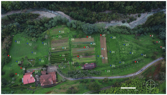
Figure 1.
Zenithal view of the study area, with the distribution of the recording stations indicated by numbered dots. The Rosaro River borders the western side of the study area in Fivizzano municipality (Northern Italy), (44°14′14.84″ N, 10°07′08.94″ E, 250 m a.s.l.). The color of each dot represents the affiliation with distinct land use categories, as derived from the cluster ordination (Figure S1) of the data in Table S1.
In recent decades, diffuse land abandonment in several parts of the Mediterranean region has produced human depopulation, decreased cultivated surfaces, and increased secondary forest cover [37,38]. In particular, the study area was intensely cultivated to produce vegetables for the local market until the 1960s. After that time, a progressive reduction in the cultivated surfaces associated with diminishing livestock rearing has progressively reduced fertilization, affecting soil structure.
Farming Activity
The area was recently designated as a rural sanctuary [37] that belongs to the “Coltura mista” practice of farming [39] and is representative of a new model of active nature conservation according to the “Earth stewardship” paradigm [40]. The area is cultivated with biological criteria all year round, producing a variety of vegetables (carrots, tomatoes, chili, peppers, eggplants, celery, artichokes, salads, onions, garlic, beans, pumpkins, potatoes, cabbages, etc.) and fruits (olives, apples, pears, apricots, kaki, figs, plums, and grapes), exclusively for family use. Twenty-seven percent of the surface is plowed by a small tractor at least once a year and is actively seeded by hand to produce vegetables. Twenty percent is mowed in July and shredded once or twice a year. Twenty-six percent of the grass is maintained as short grass all year round by shredding. Eighteen percent is kept short all year round by using periodical brushcutting. The frequency with which grasses are mainly cut depends on the amount of seasonal rain, which affects vegetative growth (i.e., increased rain = increased growth). Three percent of the land is cultivated with olive plantations, and four percent with vines. A detailed description of spontaneous vegetation and fauna is reported in Farina 2018 [37].
2.2. Site Selection
A long history of farming activity dating back at least 2000 years [41] has created a complex mosaic of soils. Forty recording stations were selected to cover the most common typologies of soils within the study area (Figure 1). We classified and characterized the sample sites within a 1-m radius plot according to the following criteria:
- (1)
- Ground slope—sloped or flat.
- (2)
- Landcover—bare soil (after recent plowing), dry meadow, wet meadow, edge (between a grove and a grass cover), grassy sloping ground, and lawn.
- (3)
- Tree cover—the presence or absence of trees.
- (4)
- Soil disturbance—estimated time interval from the last plowing event (never, far > 1 year, and recent < 1 year).
- (5)
- Vegetation and soil management—mowed, shredded, brushed, or plowed.
- (6)
- Organic matter—soil color estimation of organic content: brown (rich) or yellow ochre (poor). We classified organic matter into “rich”, “moderately rich”, and “poor”. The brown-colored soil has an average depth of 50–60 cm and is rich in organic matter. The yellow ochre soil, probably excluded by the past intense cultivation, has an average depth of 100 cm and is composed of a yellow ochre sand–clay matrix in which boulders were eliminated by repeated plowing. The yellow ochre soil is locally called “chestnut soil” because it is probably more adapted to growing chestnut trees.
Recording stations were aggregated in hierarchical clusters using the Ward method [42] (JMP® Pro 18) according to each criteria.
2.3. Environmental Variables
Temperature (Celsius) and air humidity (%) were sampled every 10 s at 10 cm depth in the soil, inside a hole 2 cm in diameter, using a PeakTech® 5185 (PeakTech, D-09212 Limbach-Oberfrohna, Germany) data logger positioned 20 cm from the recording devices. Weather data (air temperature, humidity, dew point, wind speed (m/s), wind gust (m/s), wind direction (degrees °), absolute pressure (hPa), solar radiation (lux), and hourly rainfall (mm) were collected at a resolution of one minute with a WiFi-Wetterstation, WheatherScreen Pro (Bresser GmbH, D-58507 Lüdenscheid, Germany) located in the center of the study area. Soil pH was measured with a Hanna instruments® HI 8314 analog pH meter (Hanna Instruments, Inc. 584 Park East Drive, Woonsocket, RI 02895, United States) using a soil sample collected in the same position as the soil temperature probe. High-resolution zenithal images of the study area were obtained using a DJI Mini 2® drone (DJI Innovations, 14/F, West Tower, Building 1, No. 28, Zhongguancun East Road, Haidian District, Beijing 100083, China).
2.4. Sound Sampling
We employed a C-series pro contact piezoelectric microphone (CPM) (https://jezrileyfrench.co.uk/contact-microphones.php, accessed on 24 October 2024) to detect sound vibrations. We used a Zoom F3 field recorder (2022 Zoom Corporation®, Chyoda-ku, Tokyo, Japan) powered with a INIU™ 10,000 mAh USB-C PD power bank (NIU Technologies, No. 99, Shangdi 3rd Street, Haidian District, Beijing 100085, China) to record sounds at a resolution of 32-bit float in a WAV audio format, ensuring high-quality audio capture even at low intensities. Moreover, the Zoom F3 operates with a Dual AD converter, enabling the automated recording of the loudest and the quietest sounds without adjusting the gain. A TritonAudio BigAmp Piezo 3 dB amplifier +48 V phantom powered (Herman Heijermansweg 19, 3011 VW Rotterdam, The Netherlands), belonging to a low noise Class A JFET amplifier, was applied with the piezoelectric microphone.
To increase the capacity to simultaneously capture sonic information within soils and the landscape, the piezoelectric microphone was tentatively associated with a 1.4 mm thick, 1 m long aluminum L-shaped probe. The probe’s widest arm (4 cm wide) was vertically buried in the soil, and the thinnest (1.5 cm wide) was used as a horizontal contact surface. The contact piezoelectric microphone was placed between two laminae in the center of the probe (Figure 2). A preliminary test demonstrated that this probe was more efficient than a single vertical probe measuring 20 cm in length and 4 cm in width, capturing more information within the 450 to 1200 Hz frequency range, which is critical for describing sonic activity in the soil (Figure S2).
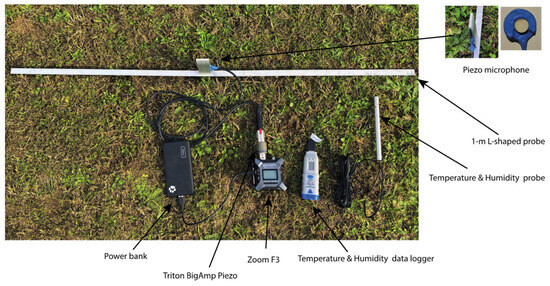
Figure 2.
1-m L-shaped probe and the recording apparatus.
Two Zoom F3 were simultaneously deployed at two adjacent (paired) recording stations. Paired sound recording devices were moved to new adjacent recording stations each day. Sound was recorded continuously for 24 h each day. The batteries and 32 GB SD (Secure Digital) cards were replaced every morning between 07:00 and 08:00 Central European Summer Time (CEST). Recordings were taken over consecutive days between 25 August and 13 September 2024 at a sample rate of 48 kHz. Stations 20 and 21 were resampled later (21 September) due to a failure in archiving the original files. Zoom F3 autonomously stored sound sequences in 3 h and 6 min files each. Due to the energy consumption required by the F3, batteries were replaced approximately every 12 h.
2.5. Data Processing and Ecoacoustic Indices
We applied a gain of +30 dB to the WAV files to enhance the detection and calculation of all collected signals. High quality recordings for analysis were achievable at this gain due to the 32-bit float resolution of the WAV files. The amplified WAV files were successively segmented into 1-min length files using Audacity® 3.6.4 free audio editor (https://www.audacityteam.org, accessed on 23 October 2024). Sonic Heterogeneity Indices (SHItf and SHIft) also known as Acoustic Complexity Indices (ACItf and ACIft), and some derivative metrics [34] were utilized to process the Fourier transform (FFT) matrices obtained by WAV files using the SonoScape™ 1.1.0426 software with a clumping parameter set to 0 [43].
An intensity filter was applied to exclude non-environmental sounds [34]. A comparison of the entire data set processed using either a 0.03 or a 0.01 filter revealed that the 0.03 filter fails to capture all signals above 6000 Hz resulting from the dB gain procedure. This observation guided our decision to use the 0.03 filter (Figure S3).
The SHItf and SHIft are based on the Canberra distance metric [44,45] and operate on a fast FFT matrix. The SHItf calculates the difference in contiguous intensities of each frequency bin along a temporal interval, so that:
where SHItf is the total sonic heterogeneity of the ith frequency bin along a time interval j, xi,j, and xi,j+1 are two contiguous values of intensity along a specific frequency bin i, and n is the number of temporal FFT intervals considered (typically segmented into 512 frequency bins separated every 46.875 Hz).
Complimentary, SHIft calculates sonic intensity across the entire frequency range (e.g., 1–24,000 Hz) at a specified temporal interval (e.g., 1 min), so that
where xi,j and xi+1,j are two contiguous intensity values of two frequency bins along each temporal step j, and m is the number of frequency bins.
Complementary to the analysis of SHIft, we examined a Spectral Sonic Signature for SHItf and a Temporal Sonic Signature for SHIft, represented as vectors derived from the sequence of their respective values [34]. The sonic signature is a popular term among musicians and intelligence analysts that refers to the sensed or interpreted sound sequences that characterize communities, locations, habitats, and ecosystems in the frequency or time domain [43,46].
Accordingly, the Spectral Sonic Signature (SSS) is obtained by averaging the total SHItf for each 512-frequency bin across all recording stations for the entire study area, which describes the frequential change of SHItf graphically:
Similarly, the Temporal Sonic Signature (TSS) is obtained by adding all SHIft values for the entire frequency range at a chosen temporal interval (e.g., 30 min, 60 min) for each recording station and the entire study area, which describes the temporal change of SHIft graphically:
Spectral Sonic Variability (SSV) is the attitude of a frequency category to assume different quantitative modalities [47]. It is calculated by applying the Gini-Simpson concentration index D to SHItf [47,48] as:
where n1 is SHItf for Spectral Sonic Variability and where S is the number of frequency bins and nl is the value of a frequency bin.
We applied the Effective Number of Frequency Bins (ENFB) to the Gini-Simpson concentration index (D). ENFB represents the effective number of equally common frequency bins necessary to produce the same heterogeneity as that observed in the sample [49]. Essentially, ENFB provides an index that reveals how sounds are effectively distributed and concentrated in the acoustic space.
We calculated ENFB as follows [34]:
Using the chord distance metric, we calculated the Sonic Signature Dissimilarity (SSD), which measures the level of spectral and temporal unevenness along the and vectors of SSS and SST, respectively [50,51]. This assumes that the maximum distance between SSS and SST vectors is no greater than √2 with 0 representing uniquely distinct vectors (i.e., absolutely dissimilar). We calculated the chord distance from non-normalized data using the following formula:
where , and are the signatures of two SHI vectors being compared; p is the number of occurrences; and y is the numerical value of the SHI in time, in the case of the SHItf (l = j), or, in the case of the SHIft, of the frequency bins (l = i).
The dendextend package and entanglement and cor.dendlist functions [52] in R [53] were used to visualize the alignment between ENFB and environmental variables in a dendrogram with the degree of association measured by the Goodman–Kruskal’s gamma coefficient (γ) [54,55]. This analysis made it possible to determine whether the pedological and environmental variables measured at recording stations were associated with the complexity and concentration of sonic information distributed across frequency bins. The entanglement is a measure between 1 (full entanglement) and 0 (no entanglement). The γ coefficient varies between (1 or −1). The closer γ is to ±1, the stronger the positive or negative association, respectively. Conversely, the closer γ is to 0, the weaker the association, with 0 representing no association.
3. Results
3.1. Data Capacity and Processing
We collected sound data from 38 recording stations over 19 consecutive days between 25 August and 13 September 2024, and 2 recording stations over 1 day on 21 September 2024. This resulted in 960 h of sound recordings separated into 57,600 one-minute WAV audio files for processing.
3.2. Environmental Features
The study area was predominantly flat across 90% of recording stations, with wet meadow (43%), dry meadow (28%), and no cover (13%) present as the three most common land cover classes. Lawns (8%), grassy slopes (5%), and hedgerows (3%) made up the remaining land cover types. Nearly 68% of the study area had tree cover classified as “far”, while less than 32% had tree cover classified as close. Soil disturbance at recording stations was relatively evenly split between “never” (47.5%) and “far” (40%), with only 12.5% of sites classified as having “recent” soil disturbance. A majority (47.5%) of recording stations underwent “shredded” landcover management, while 35% of recording stations were “brushed”; 12.5% were “plowed”, and 5% were “mowed”.
The quality of organic matter was relatively evenly distributed, with 40% of recording stations exhibiting poor quality, 32.5% of stations being moderately rich quality, and 27.5% being high quality. The average pH of the study area was 6.3 (SD = 0.6), making it mildly acidic, with a range of 5.25–7.34 (Table S1). Air temperature inside the soil ranged from 25.7 to 13.04 °C, and soil humidity oscillated between 100% and 78% (Table S2). Ambient air temperature during the sample period ranged from 33.9 °C on 30 August 2024 to 5.16 °C on 3 September 2024 (Table S3).
3.3. Sonic Sources
Based on a visual analysis of spectrograms, we tentatively categorized the sonic vibrations recorded using piezoelectric microphones into two groups: above-ground sources (sonotope) and below-ground sources (sonopedon). Sonotope sources were further divided into two types based on large and medium spatial scale sources, respectively including distant but relatively loud human-generated sounds (e.g., church bells, airplanes) and nearby sounds produced by soniferous animals (e.g., birds, insects, mammals), as well as localized human activities.
Small spatial scale sources at the grounds’ surface originated within the immediate vicinity of the horizontal arm of the probe (ranging from centimeters to a few meters). Examples included sonic emissions from arthropods like grasshoppers, vibrations caused by animal footsteps, tumbling debris moved by the wind, and the impacts of raindrops.
Vibrations within the sonopedon (i.e., below-ground sources) occurring within the soil were primarily generated by the movements and sounds made by organisms detected by the 4-cm vertical arm of the probe.
The ecotonal positioning of the 1 m-long probe—partially buried in the soil—simultaneously captured both below-ground and above-ground vibrations, effectively functioning as a sonotone device. Together, all these sources—with their inherently overlapping frequencies—combined to produce a complex spectrum of sonic energy. Figure 3 provides an example of a spectrogram derived from a 100 min recording.
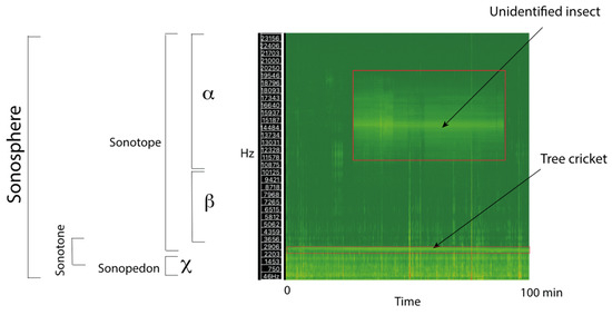
Figure 3.
Graphical representation of the elements that compose the sonosphere: sonotope, sonotone, sonopedon, and an example of a spectrogram derived from a 100 min WAV file obtained using a contact piezoelectric microphone attached to a horizontal 1 m L-shaped probe. α are large- and medium-scale spatial airborne sound waves. β are sound waves on or near the soil surface within the sonotope. χ are sound waves generated within the soil (sonopedon). α, β, and χ sound waves exhibit significant overlap in their frequency ranges. The lighter green color indicates a higher sound intensity value.
We found that a 1-m horizontal L-shaped aluminum probe effectively detected sounds within both sonopedons and sonotopes in our study area. This probe captured a substantial amount of sonic information from Types α, β, and χ, resulting in a more detailed Spectral Sonic Signature.
3.4. Spectral Sonic Signatures
3.4.1. Spectral Sonic Signature (SSS)
The Spectral Sonic Signature (SSS), obtained by cumulating and averaging all SHItf data across all 40 recording stations, showed a concentration of signals (SHItf) at the lowest frequency bins between 1 and 40 (46.87–1875 Hz) and, in a few cases, above bin 120 (5600 Hz) (Figure 4).
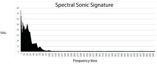
Figure 4.
Spectral Sonic Signature obtained cumulating and averaging all SHItf data across all 40 recording stations of the study area.
The temporal variation in SSS produced distinct periods of sonic activity and inactivity throughout the day where SHItf was clustered into time intervals that could be generally separated into night and twilight (0000–0600 and 1700–2300), morning (0500, 0700, and 0800), and day (0900–1600) (Figure 5). The fourth hour of the day (0400) had an SSS characterized by a uniform sound decrease due to some undefined physical events. The 20th hour of the day (2000) had a separate peak at 15 kHz, probably due to some undefined soniferous insect, as documented in Figure 3.
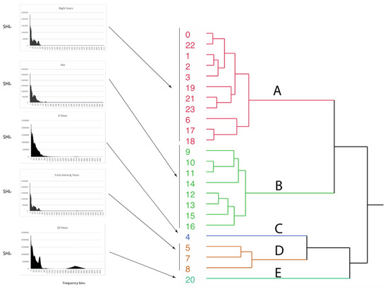
Figure 5.
Cluster analysis of the Spectral Sonic Signature (SSS) distribution across a 24-h (0–23) day cumulated for all recording stations. SHItf is the Sonic Heterogeneity Index calculated into 512 frequency bins. (A) Represents predominantly night hours and twilights (0–6 and 17–23), (B) represents predominantly day hours (9–16), (D) represents predominantly morning hours (5–8), and (C,E) represent outlying SSS associated with unidentified sonic phenomena.
3.4.2. Temporal Sonic Signature (TTS)
The Temporal Sonic Signature (TSS) displayed an undulating pattern with a maximum SHIft in the central hours of the day from 0900 to 1600 and a peak at 2000 (Figure 5). Minimum SHIft values primarily occurred during evening and dawn between 2200 and 0800 and dusk around 1700–1800 (Figure 6).
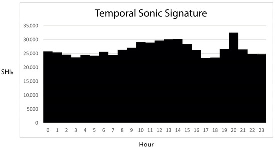
Figure 6.
Temporal Sonic Signature of average the Sonic Heterogeneity Index (SHIft) according to hours of the day (0–23).
3.4.3. Spectral Sonic Variability (SSV) and Effective Number of Frequency Bins (ENFB)
The Spectral Sonic Variability (SSV) ( = 0.975, SD: 0.002) displayed a similar but more extreme undulating trend to TSS with two peaks (at 1300 and 2000) (Figure 7A). The temporal sequencing of ENFB were concurrent with SST and SSV (Figure 7B). Specifically, 2000 h displayed the highest ENFB, followed by the fewer but notable ENFB during 0400–0600 and 0800–1600. The least ENFB were present during 1700–1800.
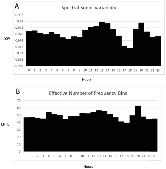
Figure 7.
(A) Spectral Sonic Variability (SSV) and (B) Effective Number of Frequency Bins (ENFB) aggregated according to the hours of the day (0–23).
The ENFB of each recording station was very weakly associated with landcover environmental variables and pedological character (entanglement = 0.41; γ = 0.08) (Figure 8).
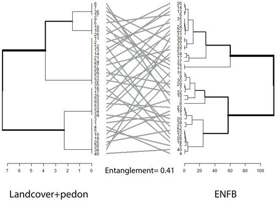
Figure 8.
The entanglement between some environmental characters (land cover and pedological fundamentals) with the Effective Number of Frequency Bins (ENFB) resulted in low entanglement (0.41), demonstrating a difference at which these two descriptors operate. Dendrograms were obtained by applying the Ward method, which minimizes within-cluster variance at each step of the process [42,52].
3.4.4. Temporal and Spectral Sonic Dissimilarity
The Temporal Sonic Dissimilarity (TSD) had a small but noticeable peak at 0300, a moderate peak at 0700, and the highest and most notable peak between 1800 and 2000 (Figure 9A). Similarly, Spectral Sonic Dissimilarity (SSD) displayed two prevalent peaks at dusk (1800–2000) and dawn (0300–0400 and 0600–0700) (Figure 9B).
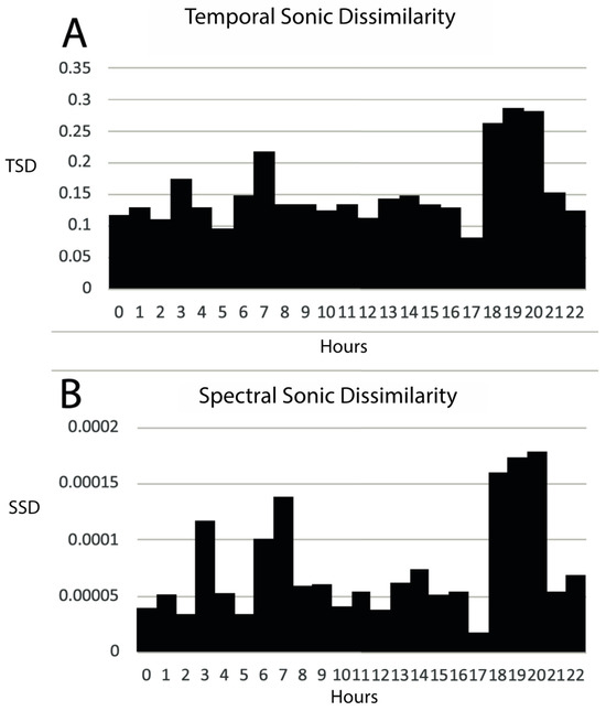
Figure 9.
(A) Temporal Sonic Dissimilarity (TSD) of SHIft and (B) Spectral Sonic Dissimilarity (SSD) of SHItf displayed over hours of the day (0–23).
4. Discussion
In Ecoacoustics, physical signals have traditionally been studied separately, classified into airborne, waterborne, and soilborne types [10]. Simultaneously, sound signals are categorized based on their source as geophonies, biophonies [56,57], or technophonies [58], with unstructured or unwanted sounds being labeled as noise [59]. Unfortunately, this approach likely limits the effectiveness of utilizing ecoacoustic indices as a comprehensive tool for ecosystem analysis while attempting to apply an oversimplification of Ecoacoustic Theory to explain complex ecological systems.
Our study aims to simultaneously examine sounds from both the soilscape and the landscape while empirically evaluating the indices commonly used in Ecoacoustic research. Recognizing the substantial differences in sound intensity between signals emitted by soil organisms and those produced by organisms above the soil, we sought to develop and test a methodology capable of capturing both low-intensity signals from the soil and high-intensity signals from the Earth’s surface. This approach facilitates a simultaneous representation and analysis of these two sonic domains, enhancing their ecological interpretation.
While airborne microphones are unable or insufficient to detect low-intensity signals within the soil, a piezoelectric (contact) microphone can capture both soilborne and airborne vibrations. However, this type of microphone significantly reduces the influence of airborne signals, as it does not capture them directly from the air. Instead, it detects the attenuated vibrations produced by these signals, which are absorbed and transmitted through a solid medium—in this case, an aluminum probe. To ensure accurate detection, signal amplification of both soil vibrations and airborne sounds, as transmitted at varying attenuation levels by the aluminum probe, is essential.
Due to the use of only two recorders at a time, our experimental design did not permit the simultaneous collection of sonic data across all stations. This limitation prevented direct comparisons of the Sonic Spectral Signature (SSS) among the 40 recording stations. However, temporal comparisons were feasible under the assumption that daily recurring processes were sufficiently consistent so as to remain unaffected by specific dates, at least within the relatively short 20-day period of our field recordings.
A SSS—representing the ‘sonic footprint’ of the study area—was derived by averaging all SHItf values across the recording sites. The SSS was primarily concentrated within the first 100 frequency bins (<4500 Hz), with two prominent peaks observed at 500 and 1000 Hz. A random inspection of selected spectrograms indicated that these frequencies were predominantly characterized by arthropod biophonies.
The absence of bird vocalizations during the daytime in late summer, combined with the lack of anthropogenic sounds at night, likely accounts for the significantly reduced sonic activity observed during this period. Through visual inspection of the spectrograms, we observed that the nightly biophony of the tree cricket (Oecanthus pellucens) produced peak levels of sonic activity. Additionally, unidentified insect biophonies were detected at several, though not all, recording stations, emerging around 0800 h and spanning frequencies between 13,000 and 18,000 Hz. An example of this biophony is illustrated in Figure 3.
We found a certain regularity in SSS across our study area, reducing the Sonic Variability one may expect among recording stations sampled on different days. These regularities resulted in a pattern of differential sonic activity observed over a 24-h day. Most notably, these patterns emerged in alignment with astronomical periods, which are, in turn, synchronized with the Earth’s rotation. Specifically, as we have mentioned above, these sonic patterns were attributable to the activity patterns of peak animal sounds at dawn and dusk, a combination of animal, human, and geophysical sounds during the day, and relatively low energy, low frequency animal and geophysical sounds at night. These sonic patterns, known as sonophases, are commonly observed in studies of airborne soundscapes [60,61,62].
When the SHItf values from all recording sites were aggregated by hour, five distinct clusters emerged. Nighttime hours displayed a unique SSS compared to both daytime and twilight hours. The unclustered positions of 0400 and 0800 h, probably caused by insect activity, remain a hypothesis at this stage.
The seemingly oscillating, wave-like pattern of the Temporal Sonic Signature (TSS) over the day coincides with those observed in studies focused on above-ground soundscapes. Our findings indicate that airborne sounds must interact with the soil. These sounds display temporal patterns attributed to human-generated sounds in the afternoon, biological sounds at dusk, and periods of low sonic activity, or natural quiet at night.
Spectral Sonic Variability (SSV) and the Effective Number of Frequency Bins (ENFB) are two interrelated measures that captured the heterogeneity of sonic information across sites within the same hourly interval. Both indices showed a pronounced peak in the middle of the day, at around 1400, as well as a secondary, isolated peak at 2000. These patterns highlight the variability of SHItf across sites when compared at the same hour of the day. Furthermore, the undulating trends observed in both indices suggest the presence of recurring sonic patterns.
The ENFB serves as a valuable proxy for comparing community soundscapes with environmental variables. A low entanglement value (e.g., 0.41) between clusters based on landcover and pedological characteristics and those based on ENFB highlights the challenges encountered in this preliminary investigation when trying to identify physical environmental factors that influence sonic activity. This apparent failure may be partly attributed to the selection of environmental parameters, whose absolute importance as predictors of the ENFB remains unknown. Additionally, the intensification procedure applied to airborne and soilborne SHItf may have negatively impacted the analysis.
We observed high values of Temporal Sonic Dissimilarity (TSD) and Spectral Sonic Dissimilarity (SSD) between 1800 and 2000. This period coincided with the onset of the dusk bird chorus, peak bat activity, and the beginning of tree cricket sounds. All of these activities were likely influenced by the variability in climatic conditions during the 20-day sampling period, which increased the distance within SHItf and SHIft values.
5. Conclusions
This preliminary investigation demonstrated the feasibility of integrating sonic information from soilborne and airborne vibrations within a sonosphere model, adopting a more ecosystemic approach to Ecoacoustics. To capture the unique ecological characteristics of the sonosphere, we utilized innovative methodologies alongside standard and traditional ecoacoustic analyses. Technically, this involved the use of a piezoelectric (contact) microphone mounted on an aluminum probe to collect vibrational signals from both soil and landscape horizons.
The sonic vibrations generated by organisms and microscopic geophysical processes in the soil occurred at such low energy levels that amplification was necessary to analyze their patterns. Similarly, the airborne signals transduced by soil via the piezoelectric microphones also needed amplification. An amplification level of 30 dB was applied to standardize two different vibrational sources, ensuring consistency for subsequent data processing. Sonic Heterogeneity Indices (SHItf, SHIft) and derivative metrics—such as the SSS, TSS, SSV, ENFB, SSD, and TSD—were effectively used to analyze the sonic data, revealing hidden patterns within the sonosphere.
Supplementary Materials
The following supporting information can be downloaded at: https://www.mdpi.com/article/10.3390/geosciences15020034/s1. Figure S1. Cluster analysis using the Ward method, based on position, land cover type, soil disturbance from plowing, land cover management, estimated organic matter, and pH of the recording stations. Figure S2. Standardized distribution of the Spectral Sonic Signature was obtained with a 4 × 1.5 × 100 cm L-shaped horizontal probe and a 4 × 20 cm vertical probe. The horizontal probe has been proved to capture more information of the frequencies between 450 and 1200 Hz that are critical to describe sonic activity in the soil. SHItf: Sonic Heterogeneity Index. Figure S3. Standardized distribution of the Spectral Sonic Signature of the entire collection of recording stations (40) processed with an intensity filter of 0.01 and 0.03. SHItf: Sonic Heterogeneity Index. Table S1. The recording stations (RS) were described according to position, landcover type, tree cover, soil disturbance by plowing (never, far > 1 yr, and recent <1 yr), plowing, land cover management, and estimated organic matter (poor, mod.rich [moderately rich], rich). Table S2. Mean and standard deviation of soil temperature and humidity at each recording station (RS). Table S3. Climatic data collected at the meteorological station located in the middle of the study area.
Author Contributions
Conceptualization, A.F. and T.C.M.; methodology, A.F.; software, A.F. and T.C.M.; validation, A.F. and T.C.M.; formal analysis, A.F. and T.C.M.; investigation, A.F.; data curation, A.F. and T.C.M.; writing—original draft preparation, A.F.; writing—review and editing, A.F. and T.C.M.; visualization, A.F. All authors have read and agreed to the published version of the manuscript.
Funding
This research received no external funding.
Data Availability Statement
Original data are available upon request from Almo Farina (almo.farina@uniurb.it).
Conflicts of Interest
The authors declare no conflict of interest. The findings and conclusions in this article are those of the authors and do not necessarily represent the views of any government agencies. Any use of trade, product, or firm names is for descriptive purposes only and does not imply endorsement by the US government.
References
- Coleman, D.C.; Callaham, M.A.; Crossley, D.A., Jr. Fundamentals of Soil Ecology; Elsevier: Amsterdam, The Netherlands; Academic Press: Burlington, MA, USA, 2017. [Google Scholar]
- Dazzi, C.; Papa, G.L. A new definition of soil to promote soil awareness, sustainability, security, and governance. Int. Soil Water Conserv. Res. 2022, 10, 99–108. [Google Scholar] [CrossRef]
- Huggett, R. Soil as part of the Earth system. Prog. Phys. Geogr. Earth Environ. 2023, 47, 454–466. [Google Scholar] [CrossRef]
- Sidle, R.C.; Gomi, T.; Usuga, J.C.L.; Jarihani, B. Hydrogeomorphic processes and scaling issues in the continuum from soil pedons to catchments. Earth-Sci. Rev. 2017, 175, 75–96. [Google Scholar] [CrossRef]
- Palmer, M.W. The coexistence of species in fractal landscapes. Am. Nat. 1992, 139, 375–397. [Google Scholar] [CrossRef]
- Buol, S.W.; Southard, R.J.; Graham, R.C.; McDaniel, P.A. Soil Genesis and Classification; John Wiley & Sons: Hoboken, NJ, USA, 2011. [Google Scholar]
- Hartemink, A.E. The definition of soil since the early 1800s. Adv. Agron. 2016, 137, 73–126. [Google Scholar]
- Killham, K. Soil Ecology; Cambridge University Press: Cambridge, UK, 1994. [Google Scholar]
- Bardgett, R.D.; Van Der Putten, W.H. Below-ground biodiversity and ecosystem functioning. Nature 2014, 515, 505–511. [Google Scholar] [CrossRef]
- Sueur, J.; Farina, A. Ecoacoustics: The ecological investigation and interpretation of environmental sound. Biosemiotics 2015, 8, 493–502. [Google Scholar] [CrossRef]
- Linke, S.; Gifford, T.; Desjonquères, C.; Tonolla, D.; Aubin, T.; Barclay, L.; Karaconstantis, C.; Kennard, M.J.; Rybak, F.; Sueur, J. Freshwater ecoacoustics as a tool for continuous ecosystem monitoring. Front. Ecol. Environ. 2018, 16, 231–238. [Google Scholar] [CrossRef]
- Farina, A.; Krause, B.; Mullet, T.C. An exploration of ecoacoustics and its applications in conservation ecology. BioSystems 2024, 245, 105296. [Google Scholar] [CrossRef]
- Oelze, M.L.; O’Brien, W.D.; Darmody, R.G. Measurement of attenuation and speed of sound in soils. Soil Sci. Soc. Am. J. 2002, 66, 788–796. [Google Scholar] [CrossRef]
- Farina, A. I: Sonic patterns III: Sounds and vibrations from soils. In Soundscape Ecology: Principles, Patterns, Methods and Applications; Springer: Berlin/Heidelberg, Germany, 2014; pp. 209–220. [Google Scholar]
- Quintanilla-Tornel, M.A. Soil Acoustics. In Ecoacoustics: The Ecological Role of Sounds; Farina, A., Gage, S., Eds.; John Wiley & Sons: Hoboken, NJ, USA, 2017; pp. 225–233. [Google Scholar]
- Maeder, M.; Gossner, M.M.; Keller, A.; Neukom, M. Sounding soil: An acoustic, ecological artistic investigation of soil life. Soundscape J. 2019, 18, 5–14. [Google Scholar]
- Rillig, M.C.; Bonneval, K.; Lehmann, J. Sounds of soil: A new world of interactions under our feet? Soil Syst. 2019, 3, 45. [Google Scholar] [CrossRef]
- Robinson, J.M.; Breed, M.F.; Abrahams, C. The sound of restored soil: Using ecoacoustics to measure soil biodiversity in a temperate forest restoration context. Restor. Ecol. 2023, 31, e13934. [Google Scholar] [CrossRef]
- Robinson, J.M.; Annells, A.; Cavagnaro, T.R.; Liddicoat, C.; Rogers, H.; Taylor, A.; Breed, M.F. Monitoring soil fauna with ecoacoustics. Proc. R. Soc. B 2024, 291, 20241595. [Google Scholar] [CrossRef]
- Zhang, M.; Crocker, R.L.; Mankin, R.W.; Flanders, K.L.; Brandhorst-Hubbard, J.L. Acoustic identification and measurement of activity patterns of white grubs in soil. J. Econ. Entomol. 2003, 96, 1704–1710. [Google Scholar] [CrossRef]
- Mankin, R.W.; Brandhorst-Hubbard, J.; Flanders, K.L.; Zhang, M.; Crocker, R.L.; Lapointe, S.L.; McCoy, C.W.; Fisher, J.R.; Weaver, D.K. Eavesdropping on insects hidden in soil and interior structures of plants. J. Econ. Entomol. 2000, 93, 1173–1182. [Google Scholar] [CrossRef][Green Version]
- Mankin, R.W.; Benshemesh, J. Geophone detection of subterranean termite and ant activity. J. Econ. Entomol. 2006, 99, 244–250. [Google Scholar] [CrossRef]
- Gamal, M.A.; Khalil, M.H.; Maher, G. Monitoring and studying audible sounds inside different types of soil and great expectations for its future applications. Pure Appl. Geophys. 2020, 177, 5397–5416. [Google Scholar] [CrossRef]
- Lacoste, M.; Ruiz, S.; Or, D. Listening to earthworms burrowing and roots growing-acoustic signatures of soil biological activity. Sci. Rep. 2018, 8, 10236. [Google Scholar] [CrossRef]
- Maeder, M.; Guo, X.; Neff, F.; Schneider Mathis, D.; Gossner, M.M. Temporal and spatial dynamics in soil acoustics and their relation to soil animal diversity. PLoS ONE 2022, 17, e0263618. [Google Scholar] [CrossRef]
- Metcalf, O.C.; Baccaro, F.; Barlow, J.; Berenguer, E.; Bradfer-Lawrence, T.; Rossi, L.C.; Vale, M.D.; Lees, A.C. Listening to tropical forest soils. Ecol. Indic. 2024, 158, 111566. [Google Scholar] [CrossRef]
- Görres, C.M.; Chesmore, D. Active sound production of scarab beetle larvae opens up new possibilities for species-specific pest monitoring in soils. Sci. Rep. 2019, 9, 10115. [Google Scholar] [CrossRef] [PubMed]
- Keen, S.C.; Wackett, A.A.; Willenbring, J.K.; Yoo, K.; Jonsson, H.; Clow, T.; Klaminder, J. Non-native species change the tune of tundra soils: Novel access to soundscapes of the Arctic earthworm invasion. Sci. Total Environ. 2022, 838, 155976. [Google Scholar] [CrossRef] [PubMed]
- Romero-Ruiz, A.; Linde, N.; Keller, T.; Or, D. A review of geophysical methods for soil structure characterization. Rev. Geophys. 2018, 56, 672–697. [Google Scholar] [CrossRef]
- Farina, A.; Mullet, T.C.; Bazarbayeva, T.A.; Tazhibayeva, T.; Polyakova, S.; Li, P. Sonotopes reveal dynamic spatio-temporal patterns in a rural landscape of Northern Italy. Front. Ecol. Evol. 2023, 11, 1205272. [Google Scholar] [CrossRef]
- Farina, A.; Mullet, T.C. Sonotope patterns within a mountain beech forest of Northern Italy: A methodological and empirical approach. Front. Ecol. Evol. 2024, 12, 1341760. [Google Scholar] [CrossRef]
- Oliveros, P. Improvisation in the sonosphere. Contemp. Music. Rev. 2006, 25, 481–482. [Google Scholar] [CrossRef]
- Xie, J.; Hu, K.; Zhu, M.; Guo, Y. Data-driven analysis of global research trends in bioacoustics and ecoacoustics from 1991 to 2018. Ecol. Inform. 2020, 57, 101068. [Google Scholar] [CrossRef]
- Farina, A. The acoustic complexity index (ACI): Theoretical foundations, applied perspectives and semantics. OIKOS 2025, 2025, e10760. [Google Scholar] [CrossRef]
- Puccinelli, A.; D’Amato Avanzi, G.; Giannecchini, R.; Nannini, D. Carta Geologica della Regione Toscana a Scala 1:10.000. Sezione 234140 Fivizzano; Regione Toscana: Tuscany, Italy, 2005; Available online: http://www.regione.toscana.it (accessed on 3 November 2024).
- Puccinelli, A.; D’Amato Avanzi, P.; Perilli, N. Carta Geologica d’Italia a Scala 1:50.000: Foglio 234 Fivizzano e Note Illustrative; ISPRA: Rome, Italy, 2010. Available online: https://www.isprambiente.gov.it/Media/carg/note_illustrative/234_Fivizzano.pdf (accessed on 13 October 2024).
- Farina, A. Rural sanctuary: An ecosemiotic agency to preserve human cultural heritage and biodiversity. Biosemiotics 2018, 11, 139–158. [Google Scholar] [CrossRef]
- Correia, T. Land abandonment: Changes in the land use patterns around the Mediterranean basin. Cah. Options Méditerranéennes 1993, 1, 97–112. [Google Scholar]
- Sereni, E. Storia del Paesaggio Agrario Italiano; Editori Laterza: Bari, Italy, 1961. [Google Scholar]
- Chapin, F.S., III; Power, M.E.; Pickett, S.T.; Freitag, A.; Reynolds, J.A.; Jackson, R.B.; Lodge, D.M.; Duke, C.; Collins, S.L.; Power, A.G.; et al. Earth Stewardship: Science for action to sustain the human-earth system. Ecosphere 2011, 2, 1–20. [Google Scholar] [CrossRef]
- Ambrosi, A. Itinerari Educativi. Lunigiana: La Preistoria e la Romanizzazione-I-La Preistoria; Centro Aullese di Ricerche e di Studi Lunigianesi: Aulla, Italy, 1981. [Google Scholar]
- Ward, J.H., Jr. Hierarchical grouping to optimize an objective function. J. Am. Stat. Assoc. 1963, 58, 236–244. [Google Scholar] [CrossRef]
- Farina, A.; Li, P. Methods in Ecoacoustics: The Acoustic Complexity Indices; Springer: Cham, Switzerland, 2022. [Google Scholar]
- Lance, G.N.; Williams, W.T. Computer programs for hierarchical polythetic classification (“similarity analyses”). Comput. J. 1966, 9, 60–64. [Google Scholar] [CrossRef]
- Lance, G.N.; Williams, W.T. Computer program for classification. In Proceedings of the ANCCAC Conference, Canberra, Australia, 16–20 May 1966. [Google Scholar]
- Blondel, P.; Dell, B.; Suriyaprakasam, C. Acoustic signatures of shipping, weather and marine life: Comparison of NE Pacific and Arctic Soundscapes. Proc. Meet. Acoust. 2020, 40, 070011. [Google Scholar]
- Gini, C. Variabilità e Mutabilità: Contributo allo Studio delle Distribuzioni e delle Relazioni Statistiche [Fasc. I.]; Tipografia di Pietro Cuppini: Bologna, Italy, 1912. [Google Scholar]
- Simpson, E.H. Measurement of diversity. Nature 1949, 163, 688. [Google Scholar] [CrossRef]
- Hill, M.O. Diversity and evenness: A unifying notation and its consequences. Ecology 1973, 54, 427–432. [Google Scholar] [CrossRef]
- Orloci, L. An agglomerative method for classification of plant communities. J. Ecol. 1967, 55, 193–206. [Google Scholar] [CrossRef]
- Legendre, P.; Gallagher, E.D. Ecologically meaningful transformations for ordination of species data. Oecologia 2001, 129, 271–280. [Google Scholar] [CrossRef]
- Kassambara, A. Practical Guide to Cluster Analysis in R: Unsupervised Machine Learning; STHDA: Marseille, France, 2017; Volume 1, Available online: http://www.sthda.com (accessed on 12 January 2025).
- R Core Team. R: A Language and Environment of Statistical Computing; R. Foundation for Statistical Computing: Vienna, Austria, 2023; Available online: https://www.R-project.org/ (accessed on 12 January 2025).
- Goodman, L.A.; Kruskal, W.H. Measures of association for cross classifications. J. Am. Stat. Assoc. 1954, 49, 732–764. [Google Scholar]
- Baker, F.B. Stability of two hierarchical grouping techniques case I: Sensitivity to data errors. J. Am. Stat. Assoc. 1974, 69, 440–445. [Google Scholar] [CrossRef]
- Krause, B. Anatomy of the soundscape: Evolving perspectives. J. Audio Eng. Soc. 2008, 56, 73–80. [Google Scholar]
- Krause, B. Into a Wild Sanctuary; Heyday Books: Berkeley, CA, USA, 1998. [Google Scholar]
- Liu, F.; Jiang, S.; Kang, J.; Wu, Y.; Yang, D.; Meng, Q.; Wang, C. On the definition of noise. Humanit. Soc. Sci. Commun. 2022, 9, 406. [Google Scholar] [CrossRef]
- Mullet, T.C.; Farina, A.; Gage, S.H. The acoustic habitat hypothesis: An ecoacoustics perspective on species habitat selection. Biosemiotics 2017, 10, 319–336. [Google Scholar] [CrossRef]
- Gage, S.H.; Axel, A.C. Visualization of temporal change in soundscape power of a Michigan lake habitat over a 4-year period. Ecol. Inf. 2014, 21, 100–109. [Google Scholar] [CrossRef]
- Mullet, T.C.; Gage, S.H.; Morton, J.M.; Huettmann, F. Temporal and spatial variation of a winter soundscape in south-central Alaska. Landsc. Ecol. 2016, 31, 1117–1137. [Google Scholar] [CrossRef]
- Mullet, T.C.; Farina, A.; Morton, J.M.; Wilhelm, S.R. Seasonal Sonic Patterns Reveal Phenological Phases (Sonophases) Associated with Climate Change in Subarctic Alaska. Front. Ecol. Evol. 2024, 12, 1345558. [Google Scholar] [CrossRef]


Disclaimer/Publisher’s Note: The statements, opinions and data contained in all publications are solely those of the individual author(s) and contributor(s) and not of MDPI and/or the editor(s). MDPI and/or the editor(s) disclaim responsibility for any injury to people or property resulting from any ideas, methods, instructions or products referred to in the content. |
© 2025 by the authors. Licensee MDPI, Basel, Switzerland. This article is an open access article distributed under the terms and conditions of the Creative Commons Attribution (CC BY) license (https://creativecommons.org/licenses/by/4.0/).