A Developed Computational Code to Build a 3D Fracture Network to Reduce the Uncertainty of Fracture Parameter Generation (A Case Study of the Emamzadeh Hashem Tunnel)

Abstract

Rock masses comprise intact rock and discontinuities, such as fractures, which significantly influence their mechanical and hydraulic properties. Uncertainty in constructing the fracture network can notably affect the outcomes of sensitive analyses, including tunnel stability simulations. Thus, accurately determining specific parameters of rock joints, including orientation and trace length, is essential. A discrete fracture network (DFN) is one technique used to simulate jointed rock. However, engineers often face challenges due to the inherent uncertainty in building a fracture network using statistical distribution functions. This study analyzed the fracture network of the Emamzadeh Hashem tunnel using MATLAB-developed code and 3DEC software. It focused on the impact of statistical distribution functions on the uncertainty of fracture network construction. The results reveal that using a negative exponential distribution can introduce significant errors in constructing the fracture network, especially when generating the dip direction. The parametric study shows that employing statistical distribution functions that account for data variance in the Probability Distribution Function (PDF) can enhance the accuracy of generating fracture parameters, such as dip, dip direction, and trace length, thereby reducing uncertainty in fracture network construction.

1. Introduction

A rock mass comprises intact rock and discontinuities such as joints, bedding, faults, and other weak planes. In many geological structures, the permeability of intact rock is significantly lower than that of fractures, which serve as primary pathways for fluid flow, including groundwater and other subsurface fluids. The presence of water within these fractures can significantly alter the mechanical and hydraulic behavior of rock masses, contributing to geohazards such as landslides, rockfalls, and tunnel instabilities. Fractures play a crucial role in determining the mechanical and hydraulic properties of rock masses, particularly in crystalline rocks with low permeability [1,2]. According to Feng [3], discontinuities’ impact on a rock mass’s engineering characteristics is much more significant than that of the intact rock. Discontinuities are critical factors in various engineering applications, influencing the strength and fluid flow quality in rock structures and leading to anisotropic and scale-dependent behavior of rock masses [4].

Various methods have been developed over the past five decades to simulate fractures. Early models represented fracture networks using three perpendicular groups of infinite planes with fixed or random spacing [5]. Poisson distribution models were later proposed to determine the distance of an infinite fracture plane from a central origin [6,7,8,9,10,11,12]. These methods often randomly generate fracture orientations or are based on dominant joint orientations, treating joints as infinite layers that do not accurately reflect the natural conditions of rock masses. Consequently, a model using finite plates was proposed to improve the Poisson plate model, making the simulations more realistic.

Hadjigeorgiou et al. [13] proposed a comprehensive engineering method to analyze the stability of vertical drilling in hard rock masses by initially generating a discrete fracture network and then combining it with the discrete element method for stress analysis. Hosseini et al. [14] developed a code to build a fracture network and investigated how joint parameters impact the construction of 3D fracture networks.

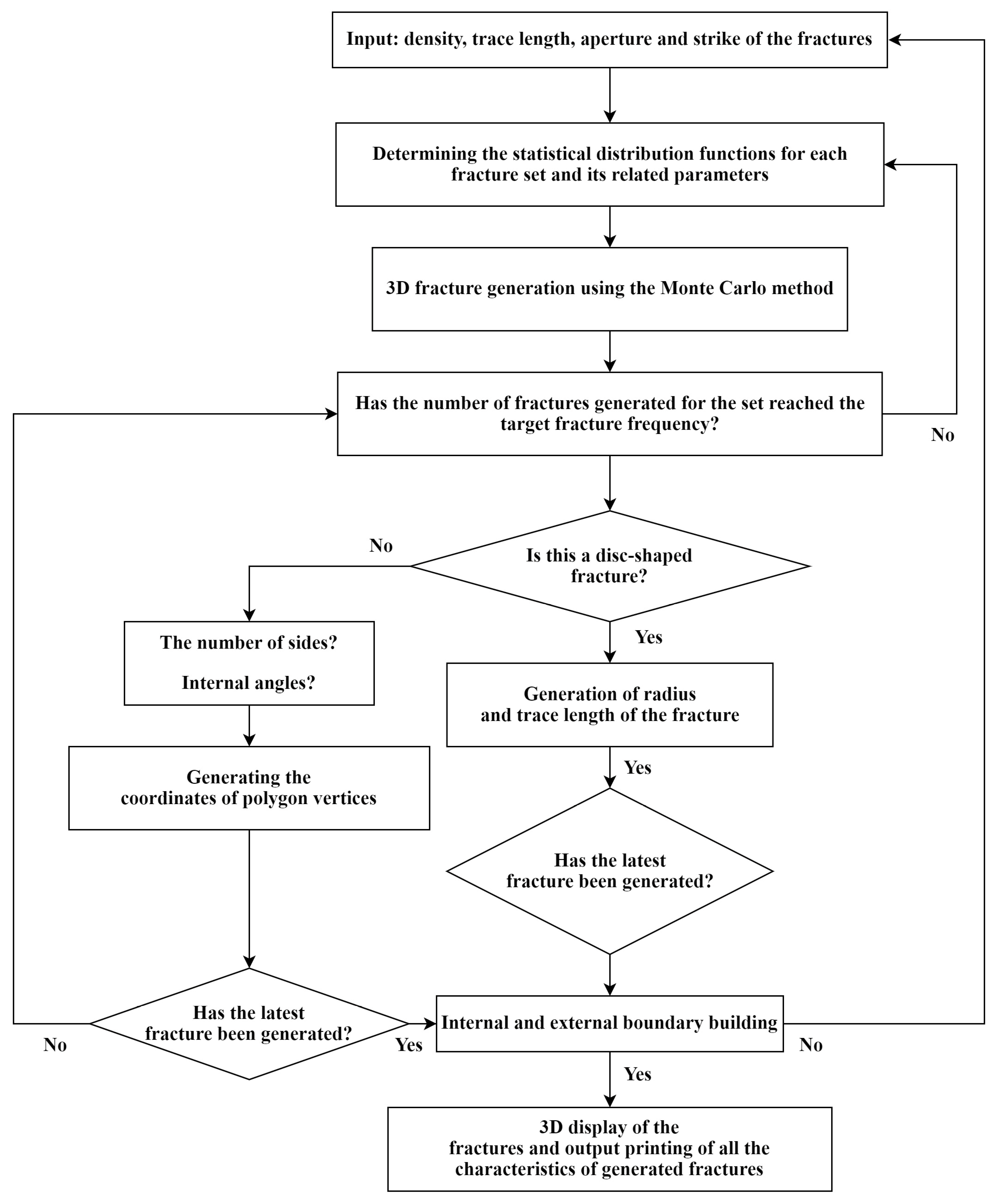
Advancements in science have led researchers to utilize new methods for simulating jointed rock masses through discrete fracture networks (DFNs). Constructing a DFN requires fracture density, orientation, length, and aperture data. The FracIUT computational code was created to produce DFNs using probability distribution functions of geometric parameters and the Monte Carlo algorithm. Noroozi et al. [15] simulated rock mass discontinuities using data from the Rudbar dam in Lorestan, while Fereshtenejad et al. [16] developed a method using three-dimensional geometry to model folded rock layers. Wang and Vecchiarelli [17] employed a geostatistical approach to model DFNs, simulating fracture density and orientation based on data from borehole walls and surface outcrops.

Constructing a fracture network based on real parameters is inherently complex. Using linear scanline or window sampling, errors such as trace line length, orientation, and density can arise when obtaining fracture data. These errors result from the limited size of the scanning or sampling window, leading to unrecorded fractures and an incomplete determination of their characteristics. Thus, it is essential to ensure that the characteristics of the obtained fracture samples closely match those of the entire fracture system. Research indicates that using statistical functions to construct a fracture network is always associated with uncertainty, posing challenges in sensitive processes such as tunnel stability. Therefore, validating the model is necessary to address these uncertainties.

This research focuses on studying the uncertainty in building a fracture network. A fracture network was generated using a MATLAB-based code employing the Monte Carlo technique. The results were then compared with those from 3DEC software (version 4.1) and data from the Emamzadeh Hashem tunnel.

Various methods have been used during the last five decades to simulate fractures. The fracture network was modeled in the early stages through three perpendicular groups of infinite planes with fixed or random spacing. Previous studies proposed the distance of an infinite fracture plane from a contracted origin via Poisson distribution models. In these methods, the fracture orientation is obtained randomly or by using the dominant joint orientation. Additionally, joints are often modeled as infinite layers, which do not accurately reflect the natural conditions of rock masses. To address this, Long et al. [18] proposed a fracture network composed of finite plates as an improvement to the Poisson plate model. This approach introduced finite longitudinal fractures with arbitrary orientations, offering a more realistic representation compared to Snow’s [5] analytical method, as discussed by Cacas et al. [19]. A comprehensive engineering method to analyze the stability of vertical drilling in hard rock masses was proposed by Hadjigeorgiou et al. [13]. The structural complexities of the rock mass were initially recorded by generating a discrete fracture network. The fracture system was subsequently combined with the discrete element method for stress analysis [13]. Hosseini et al. [14] created a code to build a fracture network and studied how joint parameters impact 3D fracture network building.

As science has advanced, researchers have utilized new methods to simulate jointed rock masses through discrete fracture networks. Building a discrete fracture network requires information on the fracture density, orientation, length, and aperture. The computational code FracIUT was created to produce a discrete fracture network via probability distribution functions of the geometric parameters of discontinuities and the Monte Carlo algorithm [20]. Noroozi et al. [15] simulated the network of rock mass discontinuities in this area via data from the Rudbar dam in Lorestan. Fereshtenejad et al. [16] proposed a method that uses three-dimensional geometry to model folded rock layers. Wang and Vecchiarelli [17] employed a geostatistical approach to model the discrete fracture network. Their study involved simulating the density and orientation of fractures via geostatistical methods, which rely on data gathered from borehole walls and surface outcrops. Zhang’s study [21] further advanced the field by presenting a novel DFN flow model that incorporates the actual connections of large-scale fractures.

Fang et al. [22] demonstrated how global sensitivity analysis (GSA) can be employed to identify discrepancies in prior Bayesian methods. They combined this with approximate Bayesian computation (ABC) and a tree-based surrogate model to align the model with production history. These methods were applied to a complex fractured oil and gas reservoir, where all uncertainties, including petrophysical properties, rock physics, fluid properties, discrete fracture parameters, and dynamic factors like pressure and transmissibility, were jointly considered. Building on these developments, DFN modeling continues to advance through the integration of sophisticated computational techniques. The inclusion of the Embedded Discrete Fracture Model (EDFM) framework, numerical reservoir simulation, and geomechanics, as noted in recent studies [23,24], marks significant progress in the field. Additionally, the application of GSA and ABC highlights the critical role of robust uncertainty quantification in DFN modeling, particularly in complex reservoir environments. These innovative approaches are expected to play a crucial role in overcoming the challenges associated with modeling fractured systems, ultimately leading to more accurate predictions and effective management of subsurface resources.

However, constructing a fracture network based on real-world parameters is inherently complex [25]. Errors frequently arise when fracture data, such as trace line length, orientation, and density, are collected using linear scanline or window sampling [26]. These errors are often due to the limited scope of the scanning or sampling window, which can lead to some fractures being overlooked and hinder an accurate representation of fracture characteristics. Ensuring that sampled fracture characteristics accurately reflect the broader fracture system is essential. Research shows that statistical methods for constructing fracture networks are inevitably accompanied by uncertainty, which presents challenges in critical applications, such as ensuring tunnel stability [27]. Consequently, validating the DFN model is crucial to address the inherent uncertainties in its construction.

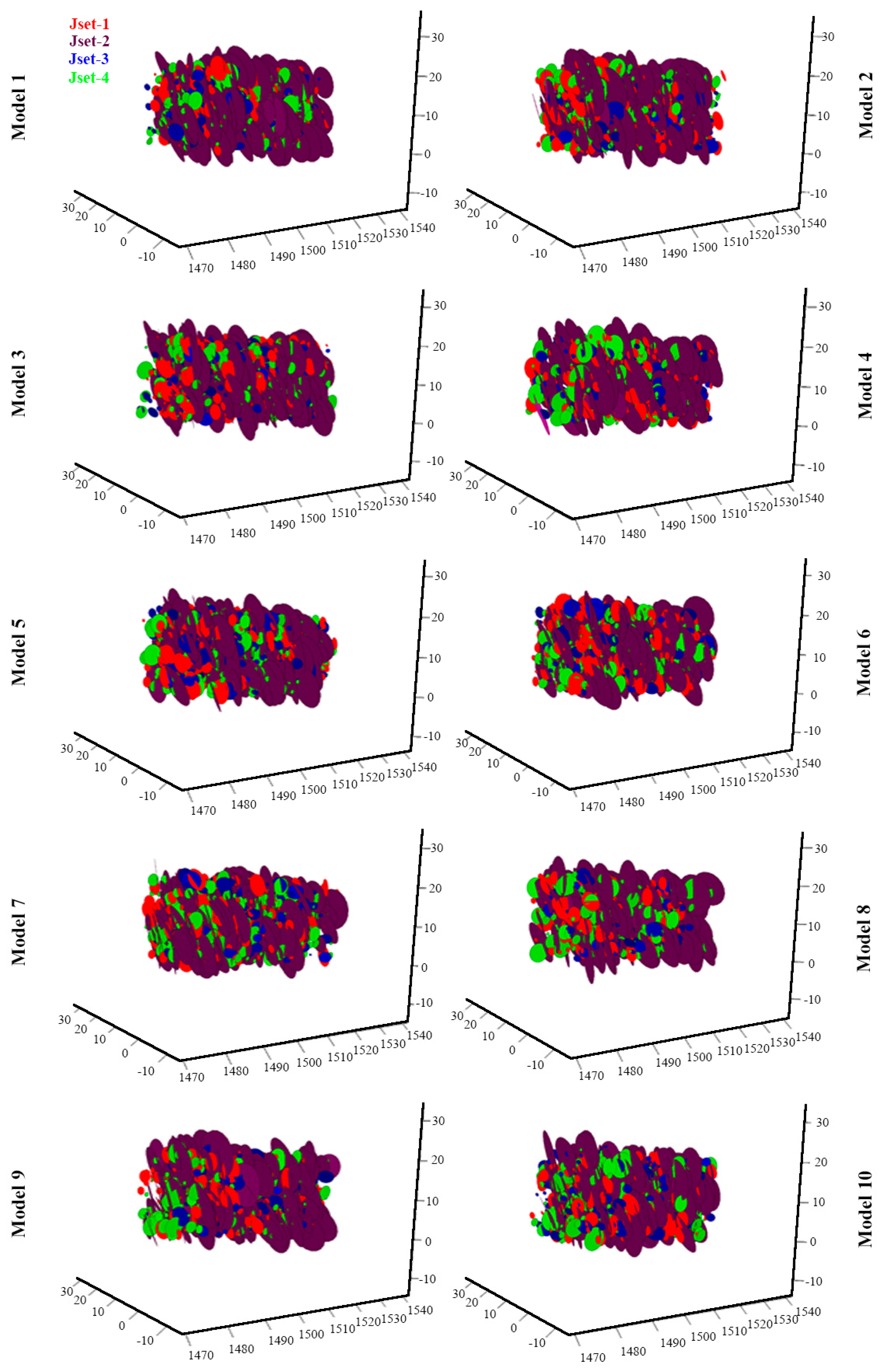
This research aims to reduce uncertainties in DFN modeling by generating a fracture network using a MATLAB-based code that applies the Monte Carlo technique. The accuracy and reliability of the generated results are then assessed by comparing them with outputs from 3DEC software and empirical data from the Emamzadeh Hashem tunnel. Estimating directional parameters, such as dip and dip direction, is essential for accurately modeling fracture networks. While traditional models, including 3DEC, are commonly used for this purpose, they often encounter limitations when processing data with complex statistical distributions or high variance, such as negative exponential and power distributions. These challenges can introduce further uncertainty into modeling outcomes, particularly when data variance is not explicitly incorporated into probability distribution functions.

To address these limitations, this study introduces a novel, customized code that enhances the accuracy of fracture network modeling. Our approach demonstrates improved precision in estimating dip and dip direction across various statistical distributions, particularly in cases where traditional models exhibit limitations. This method provides greater adaptability and reliability for geological modeling applications, especially when handling data with high variance or non-normal distributions.

2. Study Area

In this study, a 3D fracture network is built on the basis of data from the Emamzadeh Hashem tunnel. The tunnel is located in the NE of Tehran Province and is surrounded mainly by Cambrian sediments, carbonate sediments, and Jurassic sedimentary deposits. (Figure 1) depicts the general tunnel location and geological map of the Emamzadeh Hashem tunnel.

3. Materials and Methods

3.1. Development of the Code for Building a Separate Fracture Network

The geometry of a rock mass’s fracture system is a crucial factor in applied rock engineering projects. To represent the fracture system, we generated random fractures based on the statistical distributions of their geometrical parameters. Each random model represents a small part of the studied area where fractures are assumed to have the same statistical behavior. This study used the Monte Carlo simulation method to generate random samples from these statistical distributions, effectively modeling the inherent variability and uncertainty. The essential parameters for fracture network construction included orientation, length, and fracture density, typically determined through field data, borehole data, or virtual survey equipment such as LiDAR [28]. Once these parameters were established, the Monte Carlo technique created the fracture network. Previous studies have demonstrated that the Monte Carlo method effectively builds fracture networks [29]. This method simulates each fracture as a disk or parallelogram with finite dimensions in three-dimensional space. Figure 2 shows a 3D fracture network generated using our developed MATLAB code.

First, the algorithm takes fracture system characteristics like fracture density, trace length, aperture, and fracture strike as input parameters. These parameters depend on each fracture set’s statistical distribution functions and geometric properties. The fracture system’s variability and uncertainty are captured by generating random samples from these distributions using Monte Carlo simulation. The algorithm generates fractures until each set’s desired frequency is reached. Here, the algorithm determines whether each fracture is disc-shaped or polygonal. Radius and trace length are calculated for disc-shaped fractures. The algorithm determines the number of sides, internal angles, and polygon vertex coordinates for polygonal fractures. After defining the fracture geometry, the fracture is generated in 3D. The algorithm creates internal and external boundaries to fit fractures into the network.

The algorithm outputs the 3D fracture network and characteristics, allowing complete fracture system visualization and analysis. This algorithm realistically and robustly models fracture networks for geomechanical and engineering applications using the Monte Carlo method and statistical fracture parameter distributions.

3.1.1. Fracture Center Generation

Four types of point process models can be used to generate the centroid of fractures in 3D space: the homogeneous (Poisson) model, nonhomogeneous process, cluster process and Cox process [9]. Each of these models uses a specific recursive algorithm to determine the location of the fracture center by generating random numbers as the fracture centroid. This study utilized the Poisson method to generate the fracture centroid. In this method, the coordinates of the fracture plane center in three-dimensional space are as follows [30,31]:

$$x_i=x_{g1}+R_i\left(x_{g2}-x_{g1}\right)$$

(1)

$$y_i=y_{g1}+R_i\left(y_{g2}-y_{g1}\right)$$

(2)

$$z_i=z_{g1}+R_i\left(z_{g2}-z_{g1}\right)$$

(3)

where $x_{g1}$, $y_{g1}$, $z_{g1}$ and $x_{g2}$, $y_{g2}$, $z_{g2}$ represents the coordinates of the desired range, and “R_i” is a random number. An example of the coordinates of the centroid of the generated fractures is shown in Figure 3.

3.1.2. Fracture Length Generation

The fracture length is determined via the following relationship.

$$l={\left[l_{min}^{-D}+Ri(l_{max}^{-D}-l_{min}^{-D})\right]}^{-1/D}$$

(4)

l_min and l_max are the smallest and largest lengths of the fracture, D is the fractal dimension, and “R_i” is a random number [32]. The dip and dip direction of the fractures are also obtained via statistical distribution functions. The developed code can consider normal, log-normal, power, exponential and uniform statistical functions. Figure 4 shows an example of the length of the fractures generated via a power distribution function, with minimum and maximum lengths ranging from 1.5 to 4.2 m.

3.1.3. Fracture Orientation Generation

The fracture orientation includes two components: dip and dip directions. These two parameters and other fracture geometrical characteristics are generated independently and follow their statistical distributions. The developed code allows the consideration of Fisher, normal, log-normal, exponential, and uniform statistical functions to generate dip and dip directions.

3.1.4. Fracture Network Building

The developed code allows for visualizing fracture planes in three dimensions and can output each fracture’s parameters as an Excel file. In this study, using the Monte Carlo technique and based on the code developed in MATLAB R2022b, 10 random models for the Emamzadeh Hashem tunnel’s fracture network were created, shown in Appendix A Figure A1. An example of a fracture network constructed with the developed code for the identified joint sets obtained via DIPS software (version 4.1) is shown in Figure 5.

4. Discussion and Results

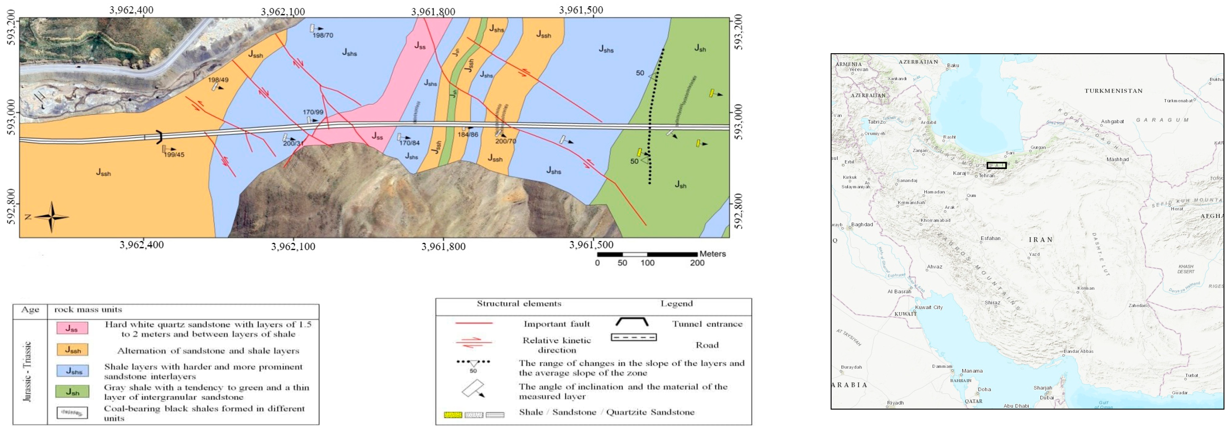
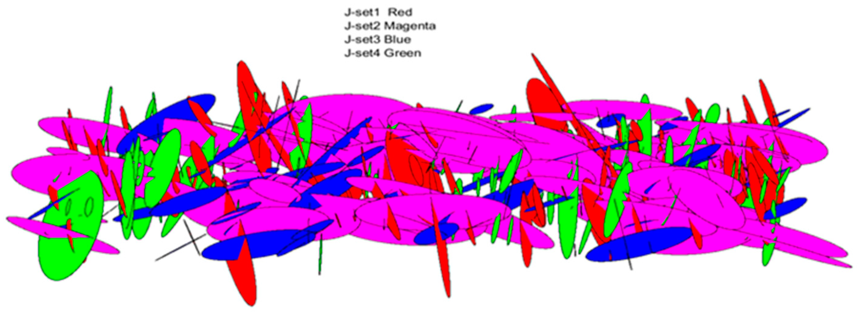
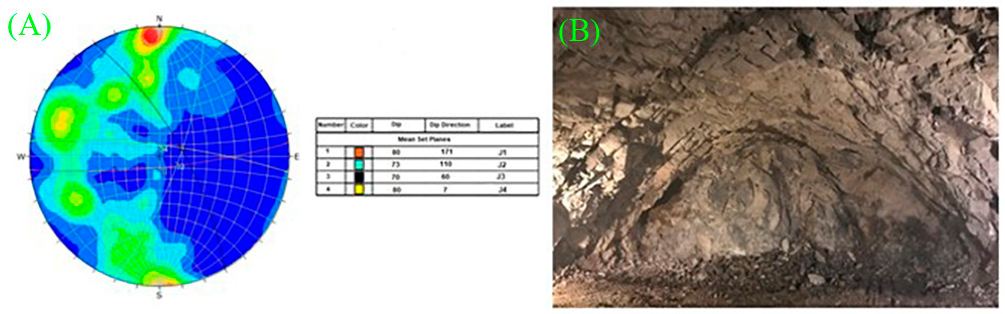
The initial step involved collecting data from the Emamzadeh Hashem tunnel in 3-m sections and then inputting them into DIPS software to model the fracture data. Four groups of dominant joints in the region were subsequently identified on the basis of the concentration and intensity of the fracture pole in various areas of the stereo net (Figure 6). The statistical functions of each joint set were determined on the basis of the fitting performed on the collected data, and these functions are presented in

Table 1. Statistical parameters of each joint set.

Joint Set	Characteristic	Distribution	Parameters
1	Dip direction	Normal	Mean = 175, Variance = 35
	Dip	Power	Min = 64, D 1 = 3.38
	Length	Negative exponential	Min = 1, Max = 10, λ 2 = 0.27
2	Dip direction	Normal	Mean = 110, Variance = 139
	Dip	Normal	Mean = 72, Variance = 98
	Length	Power	A = 23.5, D = 0.1406, Min = 0.8, Max = 8.5
3	Dip direction	Normal	Mean = 58, Variance = 104
	Dip	Normal	Mean = 66, Variance = 85
	Length	Negative exponential	λ = 0.31, Min = 1, Max = 7.9
4	Dip direction	Negative exponential	λ = 0.9341
	Dip	Normal	Mean = 81, Variance = 39
	Length	Negative exponential	λ = 0.2623, Min = 0.9, Max = 10

¹ In power distribution (x) =ax − d, the graph of f depends on a and d. ² λ: In negative exponential distribution f(x) = λe − λx, the graph of f depends on λ.

.

For Joint Set 1, the dip direction is modeled using a normal distribution with a mean of 175 and a variance of 35, indicating that the dip directions are centered around 175 degrees with moderate variability. The dip follows a power distribution with a minimum value of 64 and a D value of 3.38, suggesting that higher dip values are less frequent, starting at 64. The fracture length is characterized by a negative exponential distribution with a minimum length of 1, a maximum of 10, and a rate parameter (λ) of 0.27, indicating that shorter fractures are more common than longer ones.

Joint Set 2’s dip direction is modeled with a normal distribution, having a mean of 110 and a high variance of 139, reflecting a broad spread around the mean direction. The dip follows a normal distribution with a mean of 72 and a high variance of 98, indicating significant variability in dip angles around the mean. The length is described by a power distribution with parameters A = 23.5, D = 0.1406, and a range from 0.8 to 8.5, suggesting varied fracture lengths, with shorter lengths more frequent and a gradual decrease in frequency for longer lengths.

For joint set 3, the dip direction follows a normal distribution with a mean of 58 and a variance of 104, showing considerable spread around the mean direction. The dip is also normally distributed with a mean of 66 and a variance of 85, indicating a wide range of dip values around the mean. The fracture length is characterized by a negative exponential distribution with a rate parameter (λ) of 0.31, a minimum length of 1, and a maximum of 7.9, indicating a higher frequency of shorter fractures.

Joint set 4’s dip direction is modeled using a negative exponential distribution with a rate parameter (λ) of 0.9341, suggesting that lower dip direction values are more common. The dip follows a normal distribution with a mean of 81 and a variance of 39, indicating a relatively tight clustering around the mean dip value. The length follows a negative exponential distribution with a rate parameter (λ) of 0.2623, a minimum of 0.9, and a maximum of 10, indicating a higher likelihood of shorter fractures.

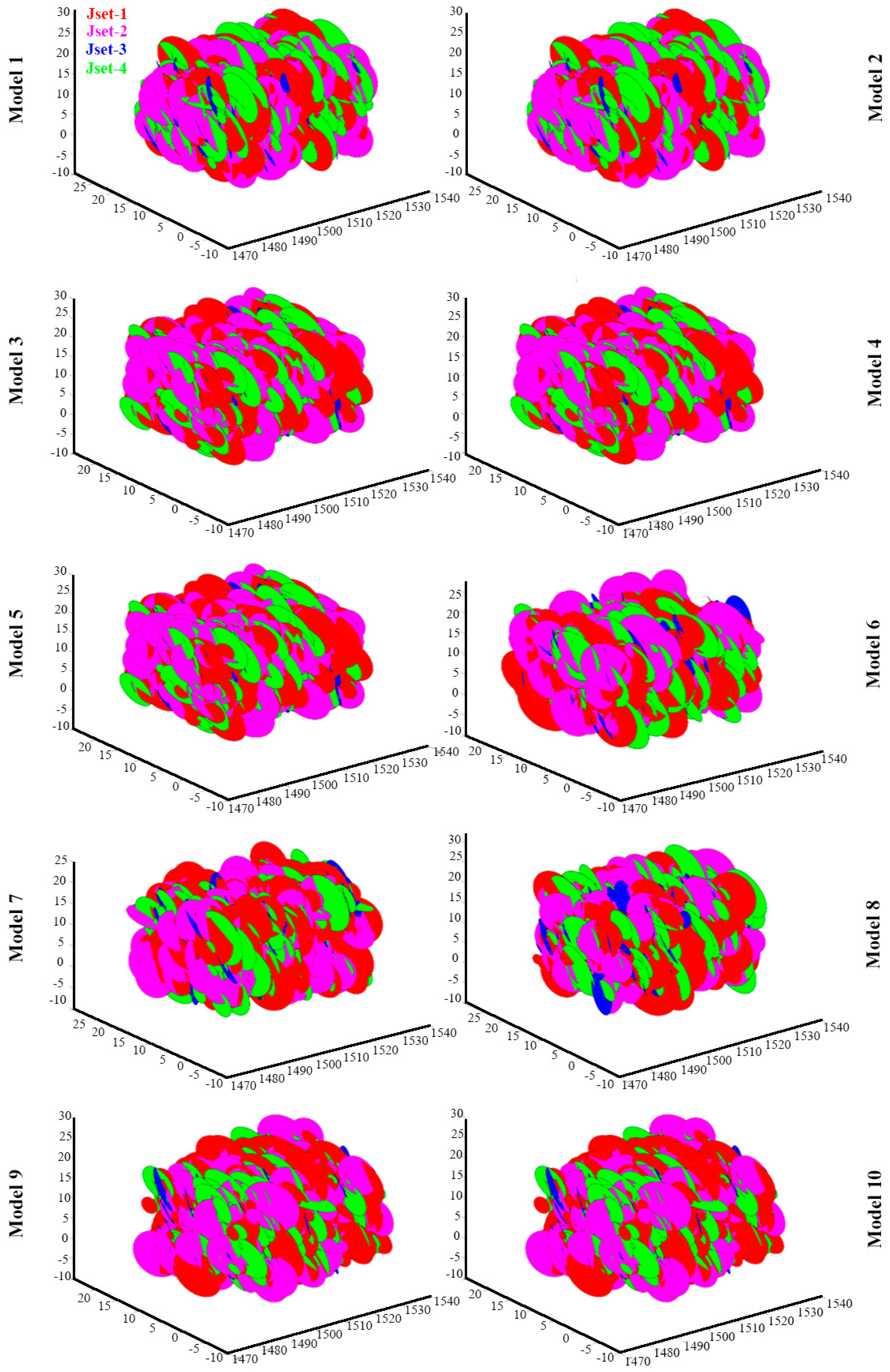
4.1. Fracture Network Building with 3DEC Software

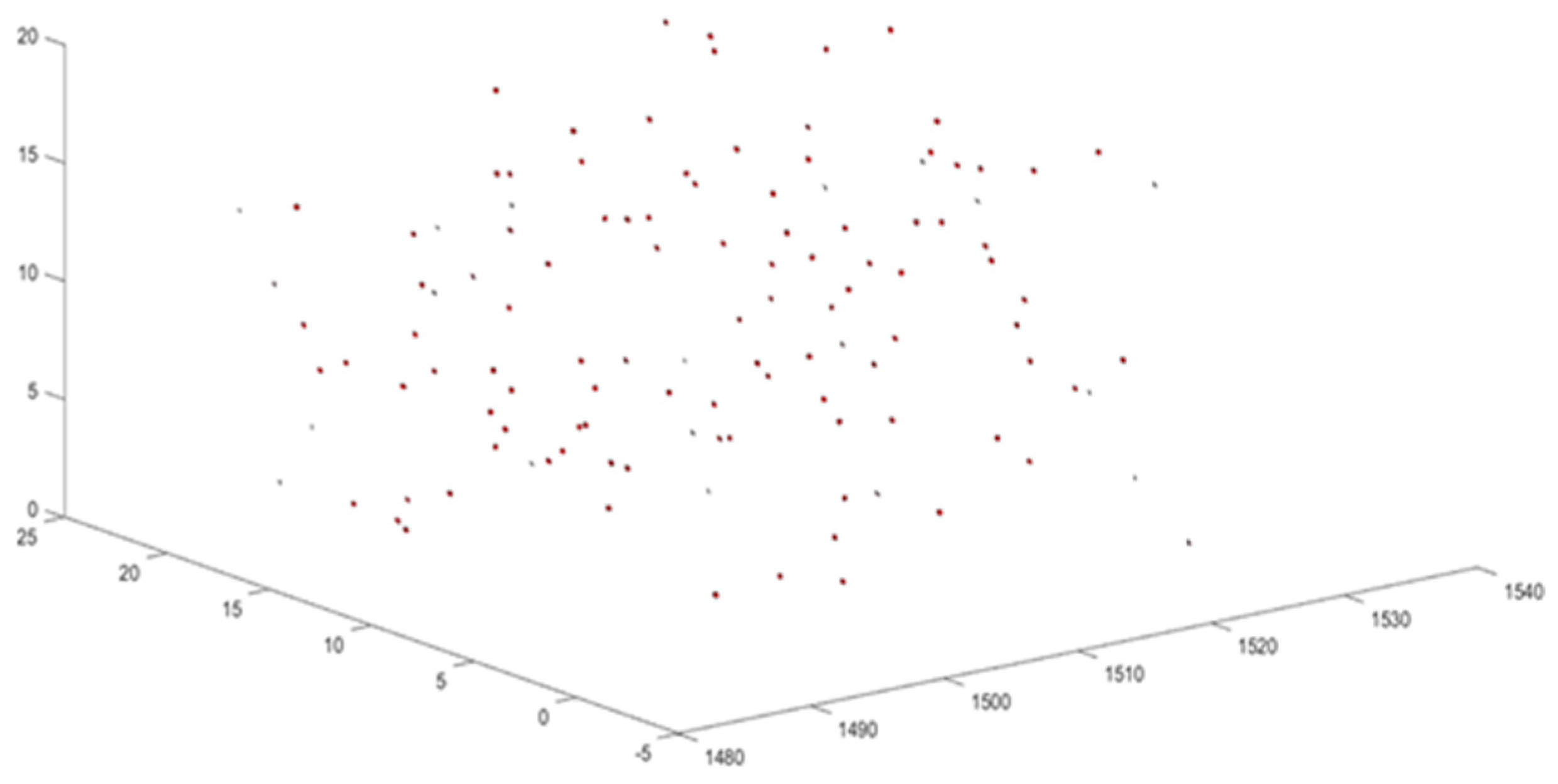
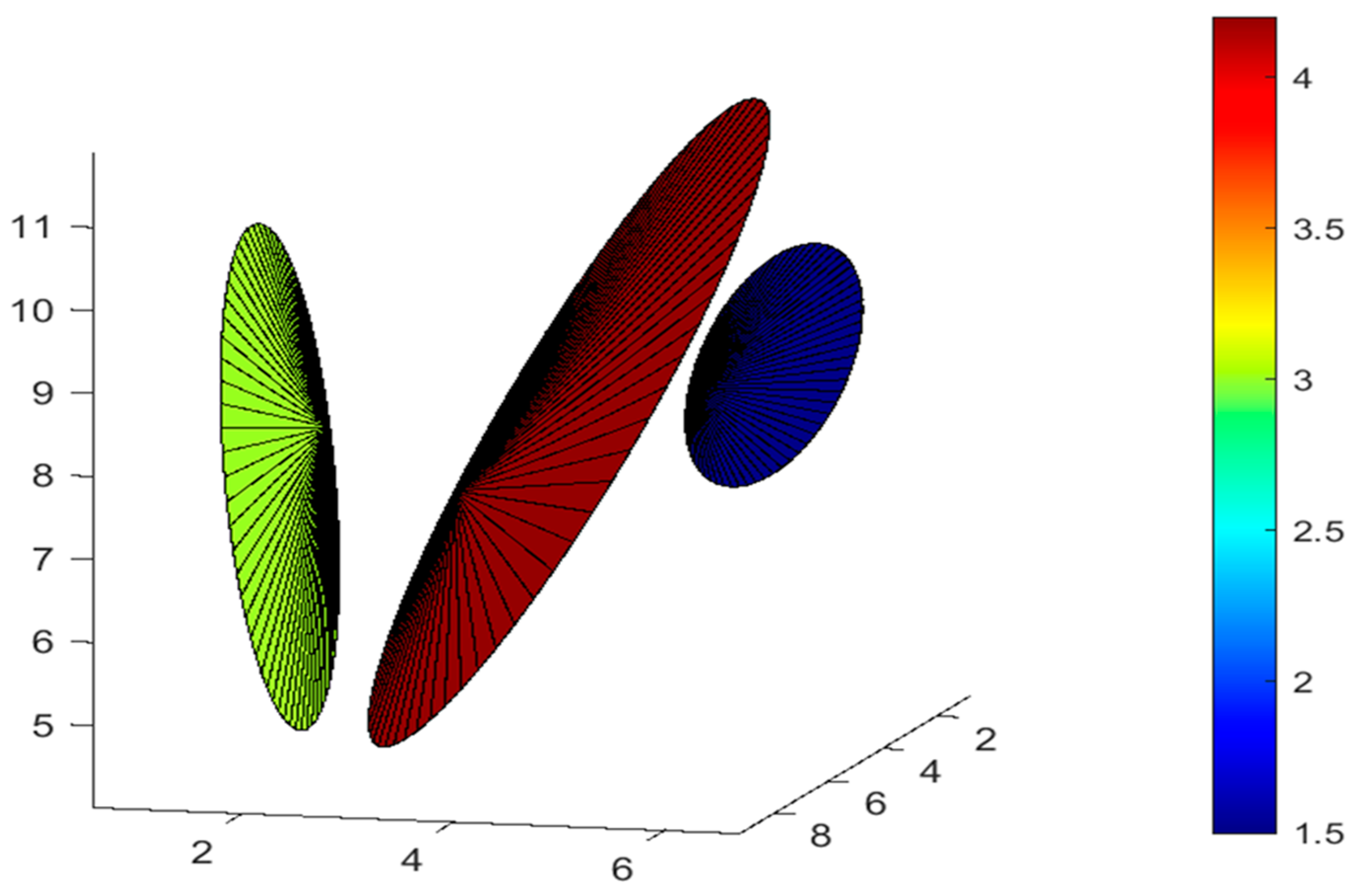
In 3DEC discrete element software, disk or parallelogram plates with limited dimensions represent fractures in 3D mode. This software can generate a fracture network on the basis of the statistical functions of fracture length, position, and orientation. Statistical functions such as power, uniform, and Gauss functions are available in this software; other functions can be developed via the FISH programming language (3DEC User’s Guide, [33]). Additionally, the density of the joint can be modeled with different modes, such as P32 (fracture plane to the volume of the sampling area) and P21 (the length of all fractures per unit area of the sampling area). Using FISH programming language in 3DEC software, 10 random fracture networks of the Emamzadeh Hashem tunnel were made, which are shown in Figure A2.

4.2. Reliability Analysis of the Discrete Fracture Network

Various methods are available to validate the fracture network. One approach involves using different sections to compare with the results of the sampling window, among other methods. Importantly, the sampling window method has drawbacks, such as the inability to remove fractures that are parallel to the window. Another approach is to compare the constructed fracture network with the input data [34]. This method involves the complete sampling of all fractures in the tunnel face. This study compared the fracture orientation, trace length, and location to the input data.

4.2.1. Fractures Direction of the Emamzadeh Hashem Tunnel

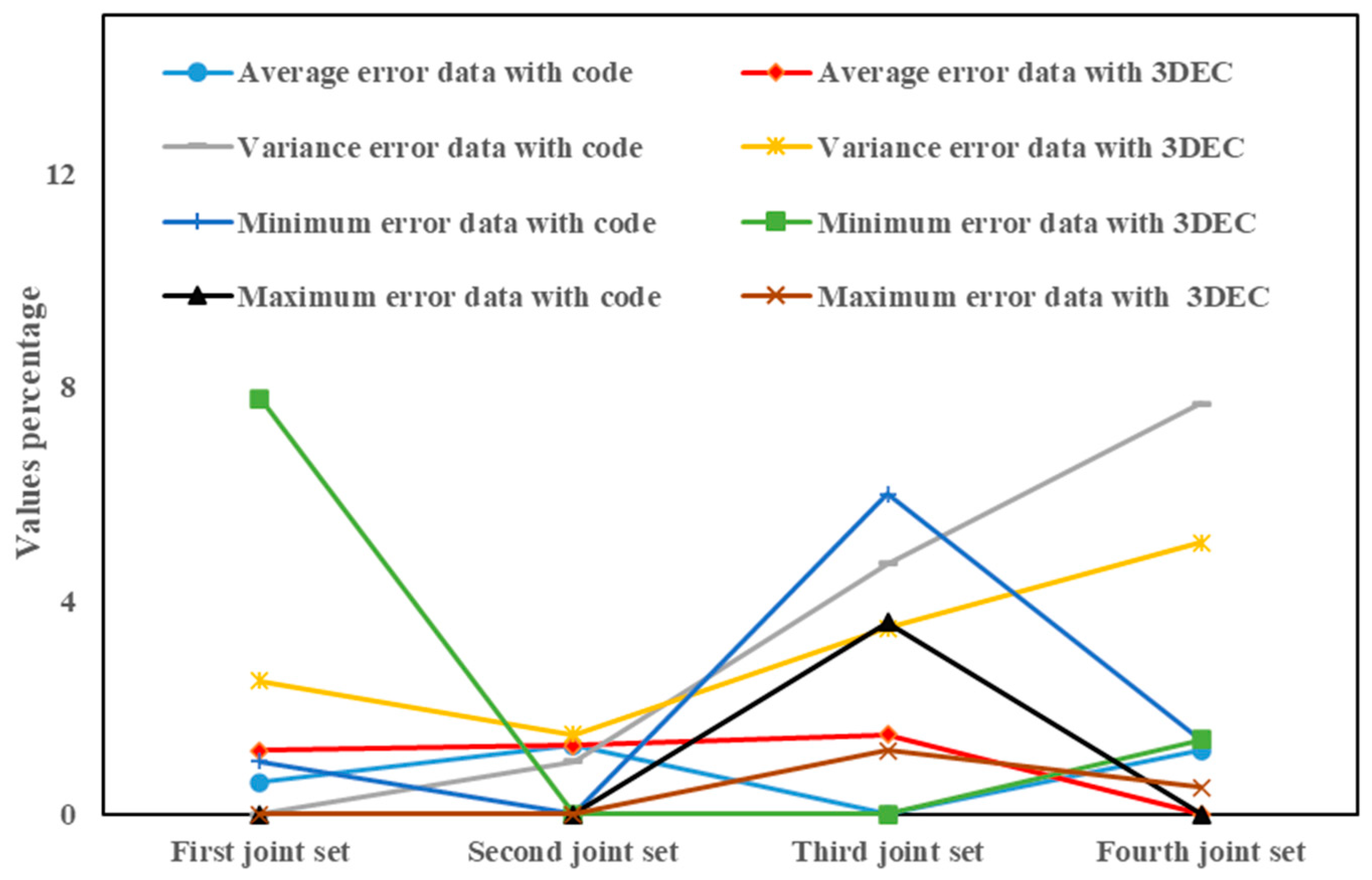
To validate the directional parameters (dip and dip directions), the primary data were compared with the results from the developed code and 3DEC software. As shown in Figure 7, the developed code generally demonstrates lower error in estimating the dip direction for the first and fourth joint sets, with only the third joint set estimated more accurately by the 3DEC software. Thus, the developed code reduces uncertainty in dip direction predictions, particularly when using a negative exponential distribution for dip direction, which does not directly account for data variance. When the data follow a normal distribution with a lower average, however, 3DEC shows greater accuracy. Both methods display the lowest accuracy with the negative exponential distribution, where the larger differences from the actual data contribute to greater uncertainty. 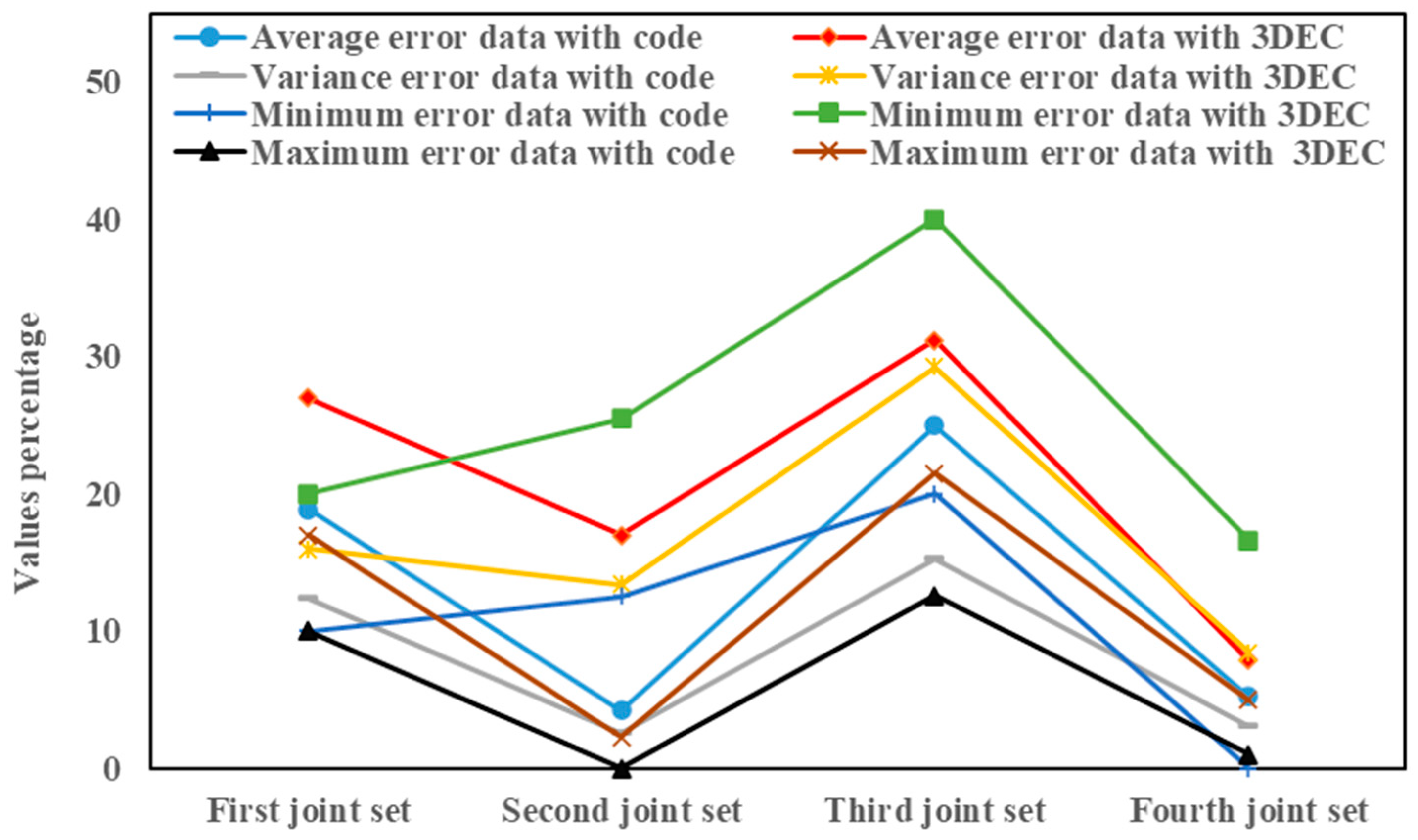Figure 8 illustrates the fracture dip results from the developed code and 3DEC software. For the first joint set with power distribution, 3DEC estimates a greater dip compared to other joint sets. Overall, the developed code performs better for exponential and power distributions, where direct handling of data variance is less critical.

Notably, the accuracy of the developed code in generating dip and dip direction decreases for normal distributions when the data have a small mean and variance. Consequently, data variance significantly influences uncertainty in fracture network construction, as higher variance generally enhances alignment between model outputs and actual data by accommodating greater variability across parameters.

4.2.2. Trace Length of Fractures in the Emamzadeh Tunnel

The comparison results of the calculated trace length are shown in Figure 9. In this figure, the difference between mean of the real data and calculated using the code(DAC) and 3DEC(DAD), difference between variance of the real data and calculated using the code(DVC) and 3DEC(DVD), the difference between minimum of the real data and calculated using the code(DMIC) and 3DEC(DMID), difference between maximum of the real data and calculated using the code(DMAC) and 3DEC(DMAD) are shown. In this instance, both methods’ most significant estimation errors are associated with the negative exponential statistical distribution function. Additionally, for the third joint set, where the average length of fractures is lower, the estimation error for both the developed code and the 3DEC software is more significant than in other cases

A comparison of Figure 7, Figure 8 and Figure 9 reveals that the most significant error of the 3DEC code and software is in calculating the fracture’s minor dip, dip direction and length values. Notably, the 3DEC code and software consistently yield accurate calculations for the maximum dip, dip direction, and length in most cases. However, the minimum values present the most significant challenge, as their calculation errors impact the accuracy of the built fracture network. Hence, their application is more suitable for creating smaller fractures. 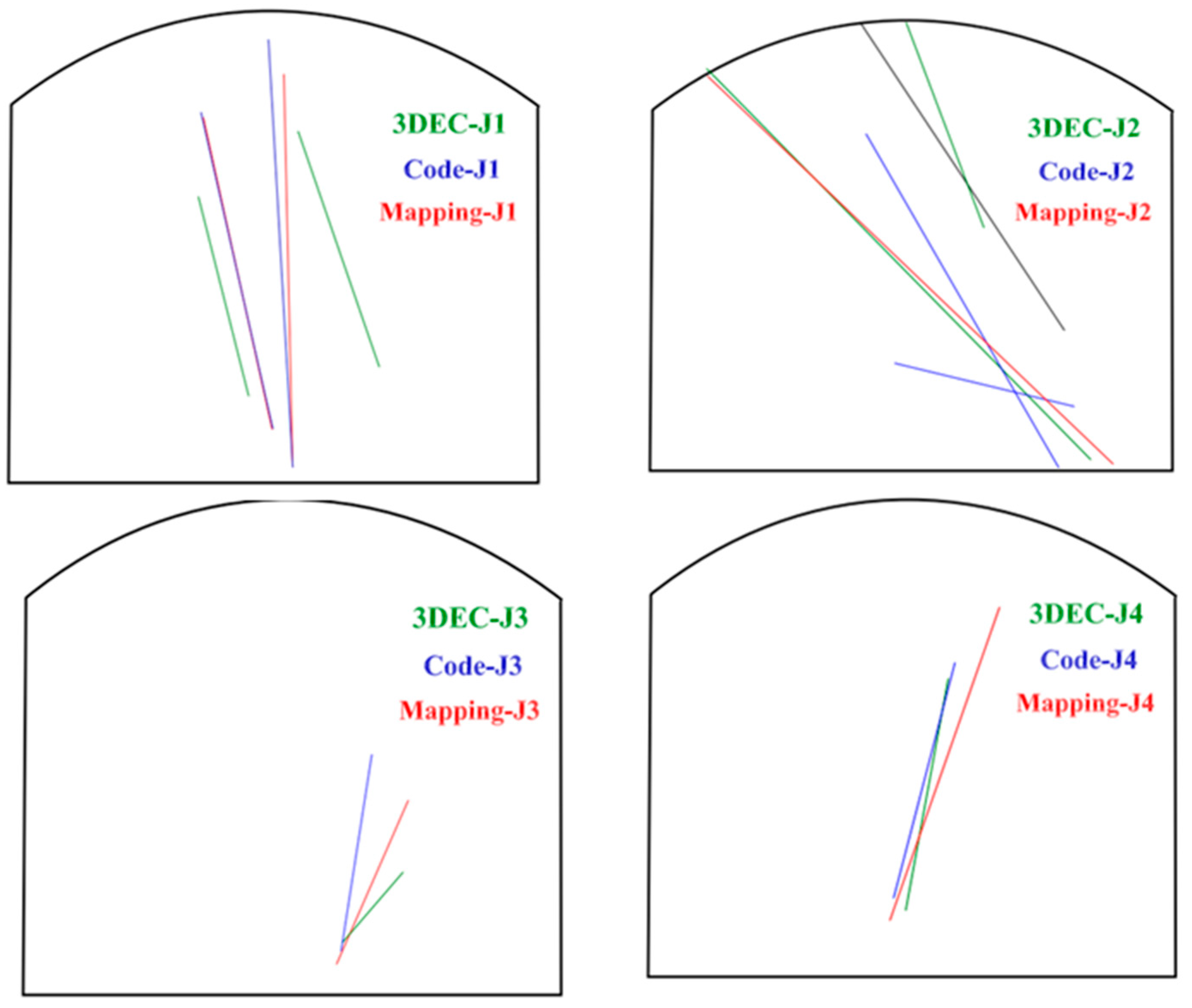Figure 10 compares the fracture production results between the developed code and the 3DEC software for a specific section of the tunnel, with a focus on the joint set. The first joint set demonstrates the closest alignment between the developed code and the actual data, indicating a strong correlation. Conversely, the second joint set exhibits the highest degree of agreement between the results obtained from the 3DEC software and the real data. Notably, the second joint set is unique among the joint sets, as none of its joint parameters adhere to a negative exponential distribution.

4.3. Parametric Study

Using a developed code, this study evaluated the impact of statistical distribution functions on uncertainty in fracture network building. Ten different scenario models for each dip, dip direction, and trace length parameter were considered on the basis of

Table 2. Various models considered for assessing uncertainty in fracture network generation.

Joint Set	Model	Distribution	Minimum	Maximum	Mean	Variance
Dip direction	1	Normal	150	175	164	35
	2	Normal	180	205	195	35
	3	Normal	100	125	114	35
	4	Normal	100	135	114	43
	5	Normal	105	125	114	25
	6	Negative exponential	15	37	26	57
	7	Negative exponential	45	6	56	57
	8	Negative exponential	100	122	111	57
	9	Negative exponential	100	122	113	30
	10	Negative exponential	105	122	113	19
Dip	1	Power	65	90	81	54
	2	Power	45	70	61	54
	3	Power	15	40	31	54
	4	Power	15	60	31	62
	5	Power	10	65	31	88
	6	Normal	70	90	78	72
	7	Normal	50	70	58	72
	8	Normal	10	32	19	72
	9	Normal	10	39	24	37
	10	Normal	15	35	25	23
Fracture length	1	Negative exponential	5	11.9	7.2	4.7
	2	Negative exponential	1	20	7.2	22
	3	Negative exponential	1	41	7.2	87
	4	Negative exponential	5	35	13	76
	5	Negative exponential	1	31	9	76
	6	Power	8.8	16.6	12.7	6
	7	Power	1	26	18.6	25
	8	Power	1	33	18.6	41
	9	Power	1	33	18.6	53
	10	Power	9	23	17	6

. This allowed us to investigate the influence of different parameters on the uncertainty in fracture network construction.

Using the data from Table 2, models 1 to 10 were constructed to compare the results of the developed code with the initial data for generating the fracture direction. Importantly, ten different fracture networks were created to eliminate random effects from each model, and the best network was selected for comparison with the actual data.

The table provides data on joint set characteristics across three attributes: dip direction, dip, and fracture length. Each attribute is analyzed through various models—normal, negative exponential, and power—with specified statistical parameters such as minimum, maximum, mean, and variance values.

4.3.1. Dip Direction

The dip direction of joint sets was evaluated using two statistical models: normal and negative exponential. For the joint sets modeled with a normal distribution (sets 1 to 5), the dip direction values range from a minimum of 100 to a maximum of 205. The mean values for these sets fall between 114 and 195, with variances ranging from 25 to 43. Notably, sets 1, 2, and 5 exhibit higher maximum values (175, 205, and 125, respectively), indicating a broader range of dip directions compared to sets 3 and 4, which share similar mean values but differ in their maximum values (125 and 135, respectively). In contrast, the joint sets modeled with a negative exponential distribution (sets 6 to 10) display a distinct range of dip direction values, with minimums ranging from 15 to 105 and maximums from 37 to 122. The mean values in this category range from 26 to 113, with variances between 19 and 57. Joint sets 6 and 7 show lower minimum values (15 and 45), while sets 8, 9, and 10 maintain higher minimum values (100 and above). The greater variance in this group suggests a more dispersed distribution of dip direction values compared to the normal model, indicating a more variable dip direction within these sets.

4.3.2. Dip

The dip attribute of the joint sets is primarily modeled using the power and normal distributions. For the power model (sets 1 to 5), the dip values range broadly, with minimums from 10 to 65 and maximums from 40 to 90. The mean values hover around 31 to 81, with variances ranging from 54 to 88. This significant variance, particularly in set 5 (88), indicates a high level of variability in the dip angles, suggesting complex geological conditions affecting these joint sets. In contrast, joint sets modeled with the normal distribution (sets 6 to 10) display dip values with a narrower range. The minimum values are between 10 and 70, and the maximum values are between 32 and 90. The means for these sets span from 19 to 78, and variances range from 23 to 72. Sets 6 and 7, with higher minimum and maximum values, suggest a more stable and predictable dip angle distribution compared to sets 8, 9, and 10, which exhibit lower minimum and maximum values and lower variances, indicating less variability in these dips.

4.3.3. Fracture Length

The fracture length of the joint sets is analyzed using the negative exponential and power models. For the negative exponential model (sets 1 to 5), fracture lengths exhibit a wide range, with minimums from 1 to 5 and maximums from 11.9 to 41. The mean values for these sets are consistently around 7.2 to 13, with variances ranging from 4.7 to 87. Notably, set 3, with a maximum value of 41 and variance of 87, indicates significant variability and longer fractures compared to the other sets in this model. Joint sets modeled with the power distribution (sets 6 to 10) show minimum values ranging from 1 to 9 and maximum values from 16.6 to 33. The means for these sets are between 12.7 and 18.6, with variances ranging from 6 to 53. Set 9 stands out with higher variance (53), indicating more variability in fracture lengths. In contrast, sets 6 and 10, with lower variances (6), suggest more consistent and predictable fracture lengths.

The analysis of joint set characteristics reveals diverse dip direction, dip, and fracture length patterns across different statistical models. The normal and negative exponential distributions for dip direction and fracture length show significant variability, reflecting complex geological processes. The power model applied to dip angles indicates considerable variability, especially in sets with higher variances. These findings provide valuable insights into the studied joint sets’ geological heterogeneity and structural complexities, informing further geological and engineering evaluations.

4.3.4. Distribution Types Influence the Uncertainty in Fracture Dip Direction Generation

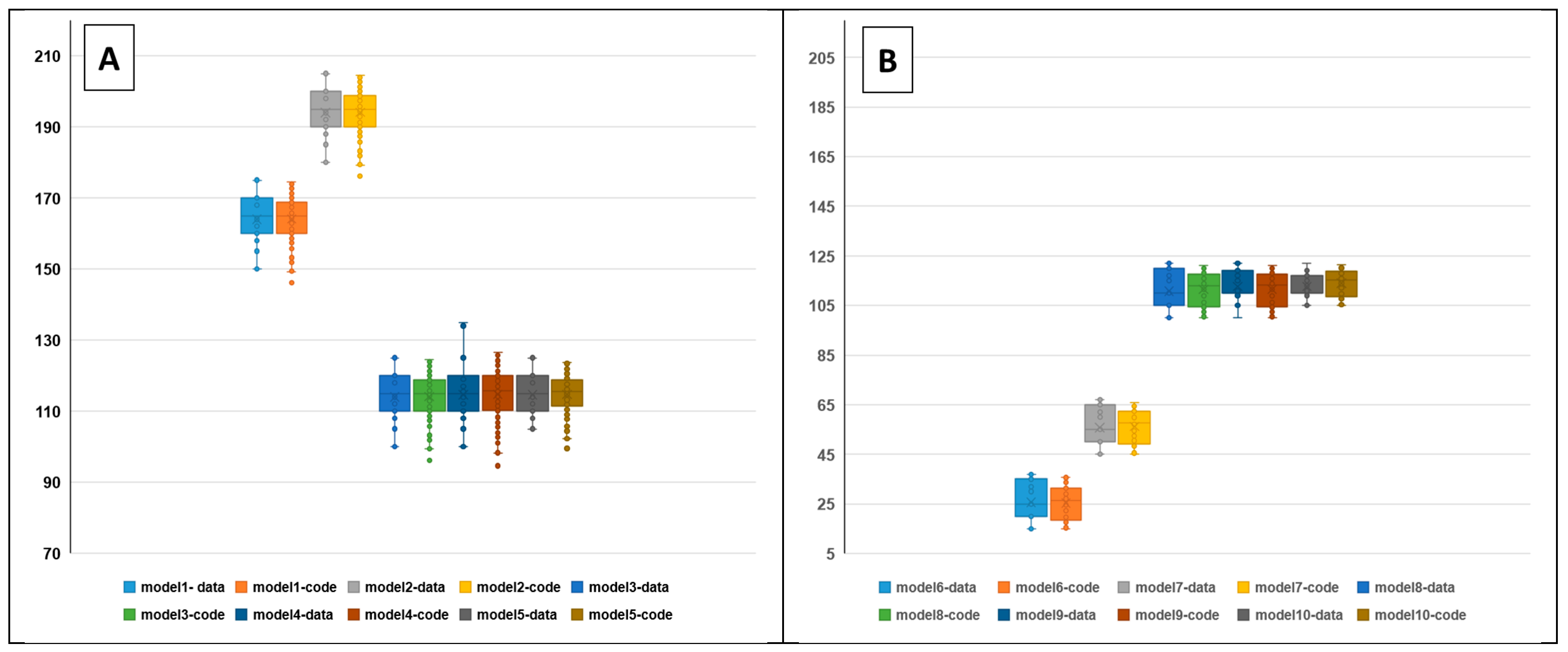
Figure 11A compares the results for the initial five models with a normal dip direction. In this diagram, the difference between the simulated values and the real values of the data is clearly shown, and it can be seen that the biggest difference between the simulated values and the real values is related to the upper or lower limit or the average of the data. The most significant difference in the performance of the developed code is observed in the dip direction calculations for the four models. These two models have the lowest average data value and the highest data variance. However, for models 1 and 2, where the average data are higher than those in the other models, the results of the developed code are very close to the real data.

The results of models 6 to 10, where the dip direction also follows the negative exponential distribution function, are shown in Figure 11B. Generally, the difference between the code results and the actual data is more significant for the exponential distribution function than for the normal distribution. One reason for this is that in the negative exponential distribution, the variance of the data is not directly considered in the PDF function. The most significant difference between the code results and actual data in estimating the fracture dip direction is related to models 9 and 10, which have a lower variance but a higher average than the other models. This point is quite different from what was observed for the normal distribution. For the minimum and maximum normal distribution, the simulated values are different from the real values, while for the negative exponential distribution, the difference is more related to the average of the data and a quarter of the second and a third of the data.

4.3.5. Fracture Dip Generation Uncertainty and Statistical Functions

Similar to the approach for fracture dip direction, various models (outlined in Table 2) have been developed to quantify the uncertainty associated with predicting fracture dip. Figure 12A compares the results obtained using our code with accurate data for the first five models, which follow a power distribution. The code accurately calculates fracture dip for models 1 to 3. However, this accuracy decreases significantly for models 4 and 5. This decline is attributable to a lower average and a higher variance in the data for these models, which aligns with the influence of a normal distribution on the generation of fracture dip.

In contrast, for the remaining five models (represented by the normal distribution in Figure 12B), reducing data variance significantly improves the code’s accuracy in calculating fracture dip. This behavior mirrors the impact of variance on dip direction prediction accuracy. The code performs better at calculating fracture dip when the normal distribution, rather than the power distribution, governs the dip.

4.3.6. Statistics’ Effect on Fracture Trace Length Uncertainty

The results of calculating the trace length of the fracture via the developed code for models that follow the negative exponential distribution are depicted in Figure 13A. For models 3 to 5, where the variance and average of the data are more significant, the accuracy of the code in generating the fracture trace length decreases. Furthermore, for other models that follow the power distribution, as the variance increases, the accuracy of the developed code in generating the trace length of the fractures decreases (Figure 13B).

5. Limitations of the Proposed DFN Algorithm

While the proposed DFN algorithm offers a robust framework for simulating and analyzing complex fracture systems in rock masses, its applicability is subject to several limitations based on varying fracturing characteristics. Firstly, the algorithm performs optimally in scenarios with moderate to high fracture densities where stochastic modeling is advantageous. In rock masses with very few fractures, explicit modeling of each fracture may provide greater accuracy, making the stochastic approach less beneficial [35].

Additionally, the algorithm assumes simplified geometric shapes for fractures, such as circles, ellipses, or polygons. This simplification may not adequately capture the intricate and irregular geometries often observed in natural fractures, potentially reducing the model’s accuracy in highly complex environments [36]. The reliance on assumed statistical distributions for fracture orientations and sizes, like the Fisher distribution for orientations and log-normal distributions for sizes and apertures, further constrains the model. Deviations from these distributions in real-world data can compromise the reliability and predictive capabilities of the algorithm [37].

Graph-based connectivity methods, such as Depth-First Search (DFS), presume that all fractures contributing to flow paths are sufficiently captured and interconnected within the model. Critical flow paths might be overlooked or misrepresented in geological settings where connectivity patterns are influenced by complex processes that are not represented in the model [38]. Moreover, identifying and removing non-conductive fractures poses challenges in heterogeneous rock masses where conductivity varies subtly, potentially affecting the accuracy of flow simulations [39].

The algorithm also differentiates between rupture and shear fractures but may not fully account for the distinct mechanical and hydraulic properties inherent to each fracture type. This limitation can impact analyses where the behavior of different fracture types significantly influences the overall system, such as in seismic response or fluid flow studies [11,40,41]. Furthermore, the algorithm is tailored for specific geological scales; applying it to significantly larger or smaller scales without appropriate adjustments may lead to scalability issues or loss of detail. The computational demands of simulating extensive and intricate fracture networks can also limit the algorithm’s practicality in resource-constrained environments [42].

Another consideration is the assumption of statistical homogeneity within defined fracture categories. This assumption may not hold in heterogeneous rock masses with varying geological features and localized variations in fracture properties, thereby reducing the model’s effectiveness in accurately capturing spatial variability [43,44]. Proper management of boundary conditions is crucial to prevent unrealistic fracture extensions beyond the physical domain, as mismanagement can introduce artefacts into the fracture network, adversely affecting subsequent analyses. Lastly, the static nature of the algorithm may not fully encapsulate dynamic geological processes and varying external stresses that influence fracture development over time, limiting its applicability in scenarios where fractures evolve due to ongoing geological or environmental changes [45].

6. Conclusions

The uncertainty in constructing fracture networks is crucial in analyses such as tunnel stability, significantly impacting simulation results. This study investigated the impact of statistical distribution functions on the accuracy of building the Emamzadeh Hashem tunnel fracture network via MATLAB and 3DEC software. The findings revealed that the most significant errors in generating joint parameters occur when the negative exponential distribution function is used. Conversely, decreasing the normal distribution’s mean and variance reduces the developed code’s accuracy in generating the dip and dip directions of fractures.

The results indicate that using the exponential distribution for the Emamzadeh tunnel fracture network can lead to substantial errors. A parametric study further examined the impact of various statistical functions on fracture parameters (dip, dip direction, and trace length). The study found that

• The use of distribution functions such as the normal distribution, which incorporates the variance of data, significantly enhances the accuracy of the developed code in generating fracture parameters.
• Decreasing the variance of the data significantly affects the accuracy of the code when the normal distribution is used.
• The most significant impact of various statistical functions is observed in generating the minimum value of fracture parameters, with the developed code accurately calculating the maximum value in most cases.
• Negative exponential and power distribution functions, where variance is not directly included, result in the most errors in generating fracture parameters.

Ensuring low variance within each joint set is essential in building fracture networks. If the variance is high, dividing the joint set into smaller sets and modeling them separately is advisable. Similar studies should be conducted for different jointing modes and density conditions to generalize these results.