Abstract
This study aims to establish a scientific and methodological basis for predicting shoreline positions using modern data analysis and machine learning techniques. The focus area is a 5 km section of the Ural coast along Baydaratskaya Bay in the Kara Sea. This region was selected due to its diverse geomorphological features, varied lithological composition, and significant presence of permafrost processes, all contributing to complex patterns of shoreline change. Applying advanced data analysis methods, including correlation and factor analysis, enables the identification of natural signs that highlight areas of active coastal retreat. These insights are valuable in arctic development planning, as they help to recognize zones at the highest risk of significant shoreline transformation. The erosion process can be conceptualized as comprising two primary components to construct a predictive model for coastal retreat. The first is a random variable that encapsulates the effects of local structural changes in the coastline alongside fluctuations due to climatic conditions. This component can be statistically characterized to define a confidence interval for natural variability. The second component represents a systematic shift, which reflects regular changes in average shoreline positions over time. This systematic component is more suited to predictive modeling. Thus, modern information processing methods allow us to move from descriptive to numerical assessments of the dynamics of coastal processes. The goal is ultimately to support responsible and sustainable development in the highly sensitive arctic region.
Keywords:
arctic; coastal retreat; permafrost; exogenous processes; Kara Sea; data analysis; machine learning 1. Introduction
Coasts composed of permafrost sediments are especially sensitive to any changes. As we know, coastal retreat rates depend on numerous environmental [1,2], climatic [3,4,5], morphological [6,7], lithological [8], permafrost [9,10,11], and anthropogenic [12] features. Studies of coastal dynamics, often focusing on regional erosion rates over varying periods [13,14,15,16], typically provide insights into the factors driving variations in erosion rates across local areas [1,3]. There is a lot of research on modeling the arctic coast [17]. The morphodynamical model of development of the arctic coasts of Russia developed by Leontiev [18,19] made it possible to quantify the transport of material influencing the rate of coastal destruction, while the model described in detail the characteristics of the storm impact and only the sediment during ice thawing in frozen soil. For the East Siberian Sea shores, the mathematical model of the sandy accumulative bar dynamics under long-term changes in open water and sea level but under unchanged permafrost, geological conditions, and atmospheric circulation has been developed and tested [20]. S.O. Razumov [21,22] developed models for developing thermal abrasion of ice banks with a stationary indicator of abrasion activity and a stable sea level, as well as under changing climate conditions. Coastal cliffs of Alaska and the Canadian part of the Beaufort Sea are exposed to active erosion, which entails virtually no beaches on the shore, and the retreat of the edge of the coastal ledges is associated with a “blocky” collapse of frozen rocks in permanent contact with sea water [23,24,25,26,27,28,29]. Thus, all approaches are regional and focused on simulating the shoreline for a particular part of the selected coast. This limits the possibilities of developing universal forecast models.
This study aims to develop a scientific and methodological basis for forecasting the position of the coastline using data analysis and machine learning methods. Artificial intelligence (AI) methods have increasingly been applied to uncover patterns in complex environmental systems. Artificial neural networks (ANNs) have been utilized in permafrost research, including studies on detecting ice-wedge polygons [30], mapping thermokarst features [31], analyzing the distribution of frozen rocks in Alaska [32], and segmenting the Alaskan coastline [33]. ANNs have also found applications in coastal studies [34,35,36,37,38]. Much AI research focuses on processing raster images, but in our study, we employ neural networks to analyze numerical data about coastal retreats.
While studying the shoreline and changes in its position, different researchers define various used shoreline indicators [39]. This study analyzes shoreline retreats by examining changes in the bluff top. Beaches and intertidal zones are not considered due to the area’s inaccessibility, the limited availability of remote sensing data, and the significant influence of tides, storm surges, etc.
According to many researchers, the main destructive coastal processes on the arctic erosion scarp are thermal abrasion and thermodenudation [40,41]. Thermal abrasion is the process of coastal destruction composed of frozen sediments under the combined influence of mechanical and thermal energy of the sea [42]. Thermodenudation is a complex of gravitational and erosive processes (collapsing, sliding, debris flow, surface wash, etc.) that develop on slopes during the thawing of permafrost deposits [43].
The arctic climate is warming significantly, accompanied by an increase in air temperatures [44] and a reduction in the period of ice cover [45,46], provoking more intensive coastal retreat [47]. Climate change also affects the land, activating cryogenic processes that transform the coastal plain and accelerate its retreat. The heterogeneity of the permafrost structure causes additional processes: thermal-erosion gullies [48] and thermokarst. Thermokarst is the thawing of ice-rich sediments and underground ice, accompanied by surface subsides and the origin of depressed landforms [49]. Thermal erosion gullies are usually initiated by ice-wedge degradation.
Traditional coastal protection methods such as gabions and fortifications made of concrete blocks, boulders, or pebbles are ineffective in arctic conditions [12,50]. A more successful approach would be to select the most stable coastal areas and identify features that characterize the zones most susceptible to retreat. In this article, we use various data analysis methods to recognize the signs characterizing areas of active coastline retreat. These methods include correlation and factor analysis, adapted for categorical and numerical data processing. Factor analysis, using field data and remote sensing on morphology, lithology, and dominant processes, can effectively assess the influence of different processes on coastline dynamics. It also helps identify areas at the highest risk of intense transformations. Unfortunately, this does not bring us closer to predicting changes in the coastline position.
When solving the forecasting problem, the question arises of what exactly should be considered the coastline position, since some changes are due to random factors associated with climatic conditions and local heterogeneities in the coast structure. The Ural coast of the Kara Sea was chosen as a case study for investigation, and an approach was created to predict shoreline retreat intensity. We selected this territory because it is characterized by high heterogeneity, even in homogeneous areas.
2. Study Area and Input Data
For the study, a 5 km section of the Ural (western) coast of Baydaratskaya Bay in the southern part of the Kara Sea was selected (Figure 1). The area is located on the coastal plain between Levdiyev and Torasavey Islands, northwest of the route where the Bovanenkovo-Uhta gas pipeline crosses the Baydaratskaya Bay. A short coastal segment will be under the influence of identical meteorological conditions. This means that wind-wave energy and the thawed index will be identical for the entire section. Their changes will occur proportionally throughout the entire area under consideration. This approach allows us to simplify the analysis of coastal zone dynamics and consider general patterns of changes within the segment.
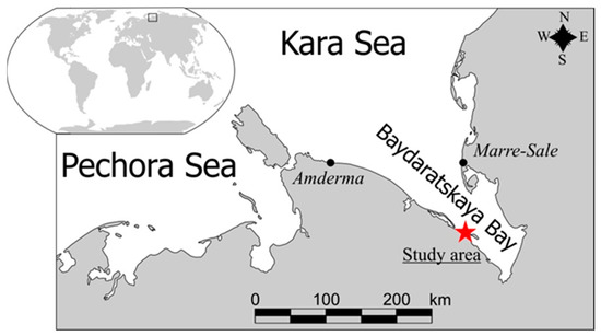
Figure 1.
Study area location. A star displays the key site; meteorological stations are shown by circles [51].
Several morphodynamic types of the coast are observed within the study area. In the central part, a lowland laida (or arctic marsh) reaches up to 3.2 m in height [52] and is periodically flooded during autumn storms and surges [53]. Thermokarst lake intensity on laida can reach 50% [54]. The western and eastern parts of the studied area feature thermal abrasion and thermodenudation coastal types, with elevations of 13–18 m in the west and 3.4–6 m in the east (Figure 2). A beach with a low-sloping gradient, ranging from 15 to 60 m wide, stretches along the coastline [51].
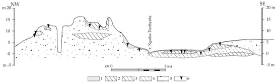
Figure 2.
Cross-section of the territory [29]: 1—peat; 2—clay; 3—interlaying of silty sand and clay; 4—silt; 5—sand; 6—ice wedges.
The coastal plain is composed of frozen Late Pleistocene–Holocene sediments [55]. The higher surfaces mainly consist of silty sands with low ice content (20–30%) [56]. The total ice content increased due to massive ground ice inclusions and ice wedges in the bluff. Exposed ground ice can reach 3.5 m in height and extend up to 80 m laterally, forming one or two layers within the coastal sections [57,58]. In the eastern part, the coast is composed of clayey sands, sandy clays, and sands, with a surface layer of ice-rich peat. The western part is dominated by ice-rich silt and clay with ice wedges (Figure 2). Permafrost processes are widely distributed in the study area.
The region experiences a severe climate. The study area is situated in the continuous permafrost zone, with a thickness ranging from 40 to 50 m and ground temperatures between −3 to −5 °C [54,59]. Different combinations of the morphological, permafrost, and lithological features of the cliff’s sediments influence the mechanism and retreat rate of the coast. These coastal features were compiled into a dataset [52]. Metadata are shown in Table 1. Previously prepared datasets were used as a data source for data analysis and machine learning methods. We considered the following periods: 1988–2005, 2005–2012, 2012–2013, 2013–2014, 2014–2015, and 2015–2017.

Table 1.
Metadata.
3. Methods
This study is divided into two independent and connected sections (Figure 3). The first section is dedicated to analyzing the data and uncovering meaningful patterns (left column). The second section utilizes a neural network to distinguish between signal and noise components in the retreat rate data.
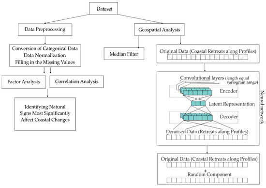
Figure 3.
Procedure of this study.
3.1. Data Preprocessing
The consideration dataset [52] contains both categorical and numerical data. Data preprocessing involves several steps. The first step involved converting categorical data into a vector for further analysis. Numerical data, such as the coordinates of the coastline position at the chosen year and the coastal retreat rate, were normalized to make them a common scale. In addition, missing data were filled in, ensuring completeness for subsequent analysis.
3.1.1. Conversion of Categorical Data
The presence of categorical data is one of the key features of the information we obtain when studying coastal dynamics and the factors influencing it. We can observe certain characteristics but cannot measure them quantitatively. For example, areas of the various predominant permafrost processes are easily identified along the Ural coast. Processes such as thermodenudation, thermal abrasion, thermal erosion gullies, and thermokarst are coded in the dataset using digital indices 1, 2, 3, and 4. These data are considered categorical because the numbers represent the classification of objects into specific groups rather than indicating any order or magnitude. A similar situation applies to lithological composition and morphological levels. Such data cannot be directly used for computational processing, which could introduce false dependencies. For instance, the indices do not imply that thermal abrasion (index 2) is greater than thermodenudation (index 1), that thermal erosion (index 3) is greater than thermal abrasion, or that the greatest process is thermokarst (index 4).
It is common to transform categorical data into a vector form for computational processing and machine learning [60,61]. In our case, we used “OneHotEncoder” preprocessors of the “Scikitlearn” library (version 1.5.1), an open-source Python 3.11.9 code [62]. The scheme of converting categorical data is shown in Figure 4.
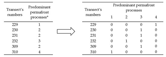
Figure 4.
Scheme of converting categorical data about predominant permafrost processes. * 1—Thermodenudation, 2—Thermal abrasion, 3—Thermal erosion gully, 4—Thermokarst.
3.1.2. Data Normalization
Normalization of data is an important step for correct comparison and ease of numerical data processing. Numerical data include the coordinates of the coastline position at the chosen year and the coastal retreat rate in different intervals.
Suppose we have three coastline positions at times T1, T2, and T3, and T3-T2 = T2-T1, i.e., the time intervals between observations are equal. Coastline changes are determined by both factors that resist destruction, such as geological, morphological, and permafrost characteristics, and factors that accelerate destruction, primarily climatic conditions [21,63,64]. These two groups of factors affect the coastal dynamics together. Suppose the coastline structure is isotropic (the same) throughout the entire area. In that case, this does not guarantee that the magnitude of the coastline retreat over the T3–T2 interval will be the same as over the T2–T1 interval. The climatic impacts at each of these time intervals may be different, which will have a greater impact on the erosion of the coast. For example, one period may have had strong storms or warm air temperatures, accelerating the coast retreat, while another may have had colder climatic conditions. Moreover, we rarely have the opportunity to observe the arctic region [65] regularly. Thus, normalization allows us to exclude variability associated with climatic impacts and focus on the features and resistance of the coastal bluff, which depend only on its geological, morphological, and permafrost characteristics.
We use minimum-maximum normalization. It is a linear conversion of the original data that adjusts the output values to the range of 0 to 1. The transformation function used for minimum-maximum normalization is as follows [66]:
where —the original data; —the normalized data; —the minimum of the original data; —the maximum of the original data.
3.1.3. Filling in the Missing Values
Most methods used in machine data processing require complete datasets without missing values, which is rarely the case in geoscience research. In coastal dynamics studies, where field observations and remote sensing methods are commonly used, missing data often arise due to limitations in their applicability. For instance, in our research, missing values occurred during a particular year when identifying the position of the bluff on the images was difficult due to peat-moss cover sliding down the slope or snow cover on the cliff caused by a snowstorm. Missing data also appeared in areas like stream mouths, rivers, and ravines along the coast, where the observation points became inaccessible.
We filled the missing values with the median value using “pandas.DataFrame.interpolate”, which fills NaN values using an interpolation method: first-degree polynomial interpolation [67].
3.2. Correlation and Factor Analysis
Despite the stochastic nature of coastline retreat, comparing images from different years reveals a consistent pattern of shoreline change. Moreover, an intuitive link between retreat rates and various structural features of the coastline can be observed. Through correlation analysis, we try to identify features that significantly correlate with changes in bluff position during 1988–2005. This period was chosen because it is long, allowing maximum averaging of local coastal features, and because it is the same as a normal distribution in retreat values (Figure 5).
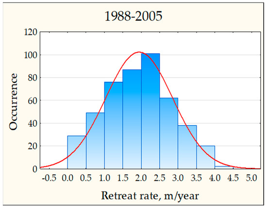
Figure 5.
The distribution of coastal retreat rates during 1988–2005 [25].
Calculating correlations between categorical and numerical requires special methods, since standard correlation coefficients apply only to the numerical data. For categorical data, metrics such as the point-biserial correlation coefficient can be used to establish a relationship between categorical and numerical data, or Cramér’s V for the association between categorical data. The correlation between categorical and numerical variables was performed using the point biserial function from the “scipy.stats” library, an open-source Python code. It is used to compute the point-biserial correlation and measures the association between a binary categorical variable and a continuous numerical variable. To assess the correlation between categorical data alone, Cramér’s V was used, which was calculated using the “chi2_contingency” function [68] from the “scipy.stats” library.
We conducted a factor analysis to identify a set of coastal features that describe the positive or negative correlations with retreat. The initial data was a matrix of categorical signs characterizing the coastal features (morphological level, type of permafrost process, and sediments composition) and the coastline retreat rates during the periods 1988–2005, 2005–2012, and 2005–2017 (Figure 6a,b,g).
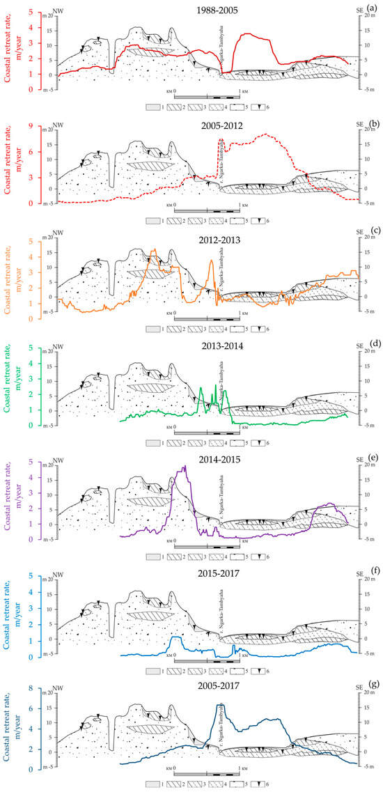
Figure 6.
Median-filtered data of retreat rates for the Ural coast during different periods: (a)—1988–2005, (b)—2005–2012, (c)—2012–2013, (d)—2013–2014, (e)—2014–2015, (f)—2015–2017, (g)—2005–2017.
Factor analysis is one of the statistical methods that help in data analysis. A factor is a hidden variable that explains the relationships between several observed parameters through their shared characteristics. This study tested various factors to identify the optimal number of factors that best explain coastal dynamics. Here, “best explains” means that factor loadings indicate the degree of correlation between each variable and factor. The higher the absolute loading, the more strongly the variable is associated with the factor. The best results were obtained using three factors. Analysis was carried out with the “factor-analyzer” module using the Promax rotation by the “FactorAnalyzer” library [69].
3.3. Approach to Predicting the Coastline Position
Due to permafrost and geological history, the Ural coast has a complex and heterogeneous structure. Upon closer assessment and zooming in on the observations, even on relatively homogeneous coastal segments, one can always detect zones (areas) of heterogeneity. These local features determine the final bluff position. A random component (or ’noise’) is always associated with variations in the coastal structure at a specific point or section of the coast. In addition, possible measurement errors and image referencing errors also introduce additional uncertainty into the data [65].
3.3.1. Median Filter and Random Component Estimation
A median filter was used in the coastal retreat rate data to account for and smooth out this random component. Each value in the data on shoreline retreat rates was replaced with the median value using a sliding window of 25 values (in our case, 250 m). This interval of the median filter is associated with the analysis of previously obtained variograms showing spatial correlations for coastal areas longer than 400 m [52]. The median filter helps to smooth out sharp outliers and eliminate the influence of random anomalies in the data (associated with permafrost and the lithological structure of the coast) while maintaining general trends.
This data smoothing procedure was performed in Excel, using a built-in function to calculate the median on selected intervals. The random component can be identified by applying a median filter, and its impact can be assessed on the original data. The next step involved calculating the difference between the original and median values to evaluate the residual (random) component.
3.3.2. Neural Network Design and Training
Using a neural network to extract noise is preferable to simple smoothing filters such as moving averages or median filters, since the neural network can capture trends and patterns in the series’ segments. A neural network has been proposed to separate random and systematic signals in a dataset of coastal retreat rates. We used an inverse convolutional network, which is usually used to extract noise in images or time series.
Inverse convolutional networks (or decoders) are an important part of the neural network architecture known as autoencoders. They are designed to restore data from a compressed representation obtained from a convolutional network (encoder). The data passes through several convolutional layers (Conv layers) in the first step. They reduce the dimensionality of the input signal and extract its main features. The encoder transforms the input data into a low-dimensional representation (latent space). In the next step, the data are passed to the decoder, which restores the original data from the compressed representation. Inverse convolutional layers (or transposed convolutions, Conv2DTranspose) increase the dimensionality of the input data, restoring spatial characteristics. They work like regular convolutional layers but are applied in the opposite order, which allows for the restoration of the resolution. The training of the inverse convolutional network occurs through the minimization of the loss function, which measures the difference between the reconstructed data and the original data. The mean squared error (MSE) is usually used for this purpose. A simple program was written in Python 3.9.17 to perform the calculations. The neural network was implemented using the “Conv1D” and “Conv1DTranspose” convolution layers of the “Keras” library. The model was trained using the “Adam” optimizer and using the mean squared error (MSE) and the “ReLU” activation layer [70].
4. Results and Discussion
4.1. Correlation and Factor Analysises
Table 2 shows the values of the correlation coefficients and the p-value, which allow us to assess the strength of the relationship and its statistical significance. The correlation between the categorical data is quite strong (Table 3), which is explained by the natural structure of the coast. The different morphological levels are composed of different lithological compositions.
Table 2.
Correlation between categorical data and coastal retreat rate.
Table 3.
Correlations between categorical data of the coast features.
The conducted correlation analysis revealed moderate and weak correlations between coastal retreat rates and various coastal characteristics, highlighting the permafrost and morphological diversity even within a small 5 km coastal segment. Study [71] examined a 10 km coastal section including the current segment; the complex and heterogeneous cryolithological, geological, and morphological structure made it difficult to identify a single dominant climatic factor, whether wind-wave energy or thermal regime. However, the article identified the wind-wave impact as the predominant influence [72]. Meanwhile, the main factor in the dynamics of this coast is thermodenudation, i.e., thermal regime (80% contribution), against wind-wave influence (20% contribution), according to [73]. The results of the correlation analysis indicate a moderately positive correlation, specifically for areas with thermokarst. In contrast, coastal retreat due to thermodenudation shows a moderately negative correlation. Coastal retreat associated with thermal abrasion, directly influenced by wind-wave energy, shows a weak correlation.
Correlation analysis represents the absence of a strong correlation, but at the same time, the presence of signs gives moderate positive and negative correlations (Table 4). This means that areas with a combination of features that have positive moderate correlations have the greatest tendency to have a rapid coastal retreat rate. The areas with negative correlation signs will be characterized by relative stability.
Table 4.
A combination of signs that have different correlations with retreat rates.
We conducted a factor analysis to identify a set of signs that have stronger positive or negative correlations. The results of the factor analysis are presented in Table 5.
Table 5.
Factor loadings during a few times along the Ural coast.
Factor (F1) associated with high shoreline change rates is linked to laida, thermokarst development, and clay deposits. The loading of coastal retreat on the factor ranges from 0.55 to 0.74 during different intervals. The strongest loading on this factor comes from the thermokarst development variable, the main indicator of rapid retreat potential in the studied area. The loading coefficient of thermokarst zones on the factor representing maximum shoreline retreat variability reaches 0.91–0.98. Consequently, the highest rates of coastal retreat are expected in areas where laida consist of loam deposits and where thermokarst processes are active. Loams are ice-rich sediments, which makes them more prone to thawing subsidence. Thawing settlement in the soil of arctic coasts ranges in huge intervals from 1% (in sandy soils) to 55% (in very ice-rich clay soils) [74]. Furthermore, due to this higher ice content, as loam thaws and is affected by marine action, fewer sediments are deposited on the coastal slope. The clay-grained and silty particles do not settle but remain suspended in the seawater. Thawing subsidence on the underwater coastal slope has been noted in numerous studies [40,75]. For the Alaska coast [40], from 1951 to 1985, 14% of the section lost was attributable to thawing sediment. The coastal zone has a thawing settlement of more than 3 m on the territory of northwest Canada [75]. The huge territory surface in Eastern Siberia (from 300 to 1000 km in length) located north of the modern coastline was significantly transformed by the developing thermokarst, where thawing settlements reached 10–35 m over the last 13–12 thousand years [76]. The rapid rates of coastal erosion are associated with the development of large thermokarst subsidences, often formed by the merger of several small thermokarst lakes [8]. The highest rates of coastal erosion in the area of recently drained lake basins were observed [77]. In addition, the drainage of lakes leads to the formation of a basin on a relatively flat surface, which in winter significantly accumulates the snow [51]. This snow accumulation also changes the surface’s heat conditions, affecting the underlying saline soils.
Laida surfaces are more vulnerable to thermal abrasion due to autumn surges and storms. However, factor analysis did not reveal quantitative evidence that thermal abrasion is leading to coastal retreat. Laida composed of sand and loam are more susceptible to thermal abrasion, but even the existing loading factor with retreat rates for data for the periods 2005–2012 and 2005–2017 are significantly lower from 0.27 to 0.33 against F1, where the correlations are 0.55–0.74 (see F2 and F3 in Table 4).
Thus, thermokarst’s important role in coast dynamics has long been known at the qualitative level. The conducted factor analysis allowed us to obtain quantitative evidence of this process for the first time. In addition, we also proposed a general algorithm for determining areas with the risk of the greatest retreat. The signs that make the most significant contribution to coastal retreat were identified based on the results of the analysis. This approach was tested for another section of the Kara Sea coast and also showed the greatest impact on the factor of coastal sections composed of clay soils.
4.2. Application of the Median Filter
Median filtering is applied to smooth out the data by reducing the impact of outliers and short-term fluctuations. The raw data have peaks and troughs (Appendix A Figure A1), indicating sudden increases or decreases in retreat rates over short distances along the coast (i.e., between adjacent transects). The extreme variations in the raw data suggest the presence of noise. This noise could result from measurement errors, short-term environmental changes, or other factors not representing the long-term trend in coastal retreat. The sharp peaks and troughs are greatly reduced or eliminated, making the overall trend more apparent. Using a median filter allowed us to smooth out random deviations without distorting the data’s overall structure on the coastal retreat rate.
Figure 6 shows the data after applying the median filter. The filtered data are much smoother than the original.
In the coastal structure, it is easier to recognize and identify areas with similar retreat rates, especially for a long time (Figure 6a,b,g). The structure generally coincides with the geomorphological level of the coast, but it is visible that the morphological structure of the coast cannot fully explain the movement of the coastline. Also, less smoothing is observed when considering short time intervals, showing heterogeneity (Figure 6c–f). Such heterogeneity is a random component. The causes of the random component may be heterogeneities of both the cryolithological structure of the coast or morphological features, and anomalous climatic events. For example, ice wedges are widespread in the studied Ural section. Its degradation in some years can be characterized by significantly higher retreat rates than in neighboring coast sections. The process may stop after the ice has completely thawed. For other sections of the Kara Sea, the rate of coastal retreat can reach 10–14 m/year during the thawing of massive ice beds [14]. Anomalous climatic events include strong storms that significantly rebuild the underwater coastal slope. Waves significantly wash out the coastal bluff in the low areas, such as laida, and the rate of destruction can reach 18–20 m/year after strong storms in other parts of the arctic region [15,78].
The histograms of the random components as a residual signal after subtracting the results of median smoothing are presented in Figure 7, and their statistical parameters are presented in Table 5.
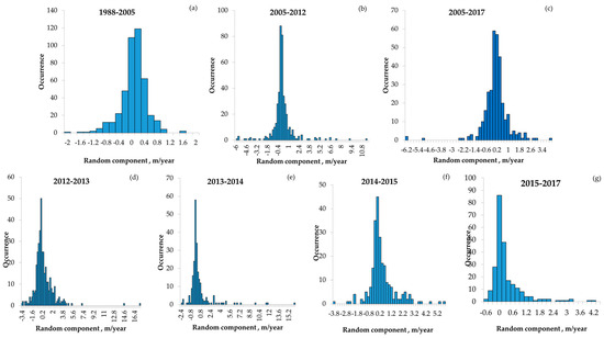
Figure 7.
The distribution of random components using a median filter: (a)—1988–2005, (b)—2005–2012, (c)—2005–2017, (d)—2012–2013, (e)—2013–2014, (f)—2014–2015, (g)—2015–2017.
The longest observation interval of 1988–2005 was characterized by minimum variance (see Table 6). Short observation periods were characterized by high variance, which emphasizes the key role in the values of shoreline retreats played by random components, which are averaged over a long observation period.
Table 6.
Main statistical parameters of the random component in the data of coastal retreat rates for the Ural coast.
Thus, considering the results of median smoothing and residual analysis, we proposed an approach where coastline destruction combines two parts. The first is a random variable associated with local variations in the coast structure and the impact of climate. The random part can be described by the distribution parameters (mean, variance, standard deviation), which allows us to establish a confidence interval. The second is a systematic shift in the average values of random distributions. The second is calculated as an average parameter.
4.3. Neural Network
As a result of working with a neural network, we learned how to separate the original signal into a useful signal (Figure 8) and noise close to a normal distribution (Figure 9).
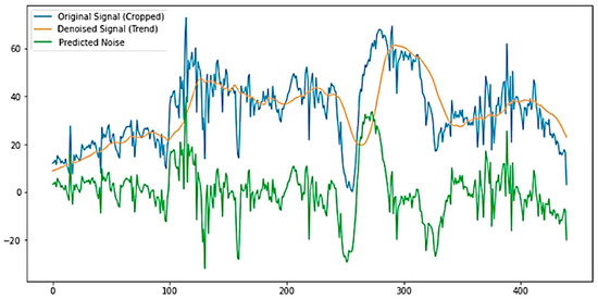
Figure 8.
The original signal, denoised signal, and prediction of the random component are used using the neural network.
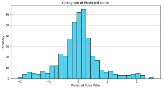
Figure 9.
The distribution of random components using neural network.
5. Conclusions
Our research has shown that combining correlation and factor analysis, incorporating categorical data, is an effective tool for assessing the impact of various processes on shoreline dynamics. This approach helps identify which natural signs most significantly affect coastal changes and pinpoint areas at the highest risk of intense transformations. It is valuable for selecting development sites in very sensitive arctic regions.
For future prediction of the coastline position, we propose to view shoreline destruction as a combination of two components: a random variable representing local shoreline variations and climate impact, and a systematic shift in the average of these random distributions. The random component can be described by its distribution parameters (mean, variance, standard deviation), enabling the establishment of confidence intervals. This first step offers a completely new approach to forecasting, based not on physical (hydrodynamic) modeling but on statistical methods. Unfortunately, there are no reliable predictive models for assessing coastal retreat in the Arctic. Everything is complicated by the presence of permafrost, which renders traditional hydrodynamic models ineffective, and the scarcity of data due to this region’s inaccessibility further aggravates the situation.
Thus, this study consists of two distinct yet interconnected parts. The first part focuses on data analysis and identifying significant patterns. The second part involves using a neural network to separate noisy data on retreat rates into signal and noise components.
Author Contributions
Conceptualization, methodology, writing—original draft preparation and editing, visualization D.B.; writing—review, supervision, S.O. All the authors have read and agreed to the published version of the manuscript.
Funding
This study was funded by the Non-commercial Foundation for the Advancement of Science and Education «INTELLECT». S. Ogorodov participation was supported by the State Research Programs 121051100167-1.
Data Availability Statement
The using datasets were made publicly available on the website https://rus.arcticcoast.ru/project_bogatova_202320251/ (accessed on 15 October 2024).
Acknowledgments
We would like to express our gratitude to our colleagues at the Laboratory of Geoecology of the North, Faculty of Geography, Moscow State University, for providing archival materials.
Conflicts of Interest
The authors declare no conflicts of interest.
Appendix A

Figure A1.
Raw data and median-filtered data of retreat rates for the Ural coast during different periods: (a) 1988–2013; (b) 2013–2017. Lines marked with “m” are median-filtered data.
References
- Irrgang, A.M.; Bendixen, M.; Farquharson, L.M.; Baranskaya, A.V.; Erikson, L.H.; Gibbs, A.E.; Ogorodov, S.A.; Overduin, P.P.; Lantuit, H.; Grigoriev, M.N. Drivers, dynamics, and impacts of changing Arctic coasts. Nat. Rev. Earth. Environ. 2022, 3, 39–54. [Google Scholar] [CrossRef]
- Lantuit, H.; Overduin, P.P.; Wetterich, S. Recent progress regarding permafrost coasts. Permafr. Periglac. Process 2013, 24, 120–130. [Google Scholar] [CrossRef]
- Ogorodov, S.; Aleksyutina, D.; Baranskaya, A.; Shabanova, N.; Shilova, O. Coastal Erosion of the Russian Arctic: An Overview. J. Coast. Res. 2020, 95, 599–604. [Google Scholar] [CrossRef]
- Hume, J.D.; Schalk, M.; Hume, P. Short-term climate changes and coastal erosion, Barrow, Alaska. Arctic 1972, 4, 272–278. [Google Scholar] [CrossRef][Green Version]
- Shabanova, N.; Ogorodov, S.; Shabanov, P.; Baranskaya, A. Hydrometeorological forcing of western Russian Arctic coastal dynamics: XX-century history and current state. Geogr. Environ. Sustain. 2018, 11, 113–129. [Google Scholar] [CrossRef]
- Manson, G.K.; Solomon, S.M. Past and Future Forcing of the Beaufort Sea Coastal Change. Atmos. Ocean 2007, 45, 107–122. [Google Scholar] [CrossRef]
- Henqutte, A.; Desrosiers, M.; Hill, P.R.; Forbes, D.L. The influence of coastal morphology on shoreface sediment transport under storm-combined flows, Canadian Beaufort Sea. J. Coast. Res. 2001, 17, 507–516. [Google Scholar]
- Hopkins, D.M.; Hartz, R.W. Coastal Morphology, Coastal Erosion and Barrier Islands of the Beaufort Sea, Alaska; U.S. Geological Survey Open-File Report 78-106354; U.S. USGS Publications Warehouse Geological Survey: Reston, VA, USA, 1978; p. 54.
- Mackay, J.R. Ice wedge cracks, Garry Island, N.W.T. Can. J. Earth Sci. 1974, 1, 1366–1383. [Google Scholar] [CrossRef]
- Vasiliev, A.A. Permafrost controls of coastal dynamics at the Marre-Sale key site, western Yamal. In Proceedings of the 8th International Conference on Permafrost: Permafrost, Zurich, Switzerland, 20–25 July 2003; Philips, M., Springman, S., Eds.; Swets & Zeitlinger: Lisse, The Netherlands, 2003; Volume 2, pp. 1173–1178. [Google Scholar]
- Lantuit, H.; Pollard, W.H. Temporal stereophotogrammetric analysis of retrogressive thaw slumps on Herschel Island, Yukon Territory. Nat. Hazards Earth Syst. Sci. 2005, 5, 413–423. [Google Scholar] [CrossRef]
- Ogorodov, S.A. Human impacts on coastal stability in the Pechora Sea. Geo-Mar. Lett. 2005, 25, 190–195. [Google Scholar] [CrossRef]
- Jones, B.; Farquharson, L.; Baughman, C.; Buzard, R.; Arp, C.; Grosse, G.; Bull, D.L.; Günther, F.; Nitze, I.; Urban, F.; et al. A decade of remotely sensed observations highlight complex processes linked to coastal permafrost bluff erosion in the Arctic. Environ. Res. Lett. 2018, 1, 38–45. [Google Scholar] [CrossRef]
- Kritsuk, L.N.; Dubrovin, V.A.; Yastreba, N.V. Some results of integrated study of the Kara Sea coastal dynamics in the Marre-Sale meteorological station area, with the use of GIS technologies. Earth’s Cryosphere 2014, 4, 59–69. [Google Scholar]
- Sinitsyn, A.; Guégan, E.; Shabanova, N.; Kokin, O.; Ogorodov, S. Fifty Four Years of Coastal Erosion and Hydrometeorological Parameters in the Varandey Region, Barents Sea. Coast. Eng. 2020, 157, 103610. [Google Scholar] [CrossRef]
- Pizhankova, E.I.; Dobrynina, M.S. The dynamics of the Lyakhovsky Islands coastline (results of aerospace image interpretation). Earth’s Cryosphere 2010, 4, 66–79. [Google Scholar]
- Frederick, J.M.; Thomas, M.A.; Bull, D.L.; Jones, C.; Roberts, J.D. Evaluating Approaches to a Coupled Model for Arctic Coastal Erosion, Infrastructure Risk, and Associated Coastal Hazards; Presented at the AGU Fall Meeting, San Francisco, USA, December 2016; Poster Number EP13C-1043. Available online: https://www.researchgate.net/publication/312167767_Evaluating_Approaches_to_a_Coupled_Model_for_Arctic_Coastal_Erosion_Infrastructure_Risk_and_Associated_Coastal_Hazards (accessed on 15 October 2024).
- Leont’ev, I.O. Modeling the evolution of the Accumulative Shores of the Barents and Kara Seas. Geomorphologiay 2002, 1, 53–64. (In Russian) [Google Scholar]
- Leont’ev, I.O. Modeling the evolution of Russian Arctic Shorelines. Oceanologiya 2004, 44, 457–468. (in Russian). [Google Scholar]
- Pavlidis, Y.A.; Leont’ev, I.O. Prognosis of East Siberian shore development on the increase of sea level and climatic change. Bull. RFBR 2002, 4, 53–57. (In Russian) [Google Scholar]
- Razumov, S.O. Thermal abrasion rate of sea coasts as a function of the climatic and morphological characteristics of the coast. Geomorphologiya 2000, 3, 88–94. (In Russian) [Google Scholar]
- Razumov, S.O. Modeling of the coastal erosion of the Arctic seas in changing climatic conditions. Kriosf. Zemli 2001, 1, 53–60. (In Russian) [Google Scholar]
- Kobayashi, N. Formation of thermoerosional niches into frozen bluffs due to storm surges on the Beaufort Sea Coast. J. Geophys. Res. 1985, 90, 11983–11988. [Google Scholar] [CrossRef]
- White, F.M.; Spaulding, M.L.; Gominho, L. Theoretical Examples of the Various Mechanisms Involved in Iceberg Deterioration in the Open Ocean Environment; Technical Report; National Technical Information Service Publication: Springfield, VA, USA, 1980.
- Russell-Head, D.D. The melting of free-drifting icebergs. Ann. Glaciol. 1980, 1, 119–122. [Google Scholar] [CrossRef]
- Holland, P.R.; Jenkins, A.; Holland, D.M. The response of ice shelf basal melting to variations in ocean temperature. J. Clim. 2008, 21, 2558–2572. [Google Scholar] [CrossRef]
- Kobayashi, N.; Aktan, D. Thermoerosion of frozen sediment under wave attack. J. Waterw. Port Coast. Ocean. Eng. 1986, 112, 140–158. [Google Scholar] [CrossRef]
- Kobayashi, N.; Vidrine, J. Combined Thermal-Mechanical Erosion Processes Model; Research Report No. CACR-95-12; Center for Applied Coastal Research: Newark, DE, USA, 1995.
- Baird & Associates. Development of a Model for the Thermal-Mechanical Erosion on Arctic Coasts; Final report prepared for Geological Survey of Canada; Geological Survey of Canada: Oakville, ON, Canada, 1995.
- Zhang, W.; Witharana, C.; Liljedahl, A.K.; Kanevskiy, M. Deep Convolutional Neural Networks for Automated Characterization of Arctic Ice-Wedge Polygons in Very High Spatial Resolution Aerial Imagery. Remote Sens. 2018, 10, 1487. [Google Scholar] [CrossRef]
- Huang, L.; Liu, L.; Jiang, L.; Zhang, T. Automatic Mapping of Thermokarst Landforms from Remote Sensing Images Using Deep Learning: A Case Study in the Northeastern Tibetan Plateau. Remote Sens. 2018, 10, 2067. [Google Scholar] [CrossRef]
- Campbell, S.W.; Briggs, M.; Roy, S.G.; Douglas, T.A.; Saari, S. Ground-penetrating radar, electromagnetic induction, terrain, and vegetation observations coupled with machine learning to map permafrost distribution at Twelvemile Lake, Alaska. Permafr. Periglac. Process 2021, 32, 407–426. [Google Scholar] [CrossRef]
- Aryal, B.; Escarzaga, S.M.; Vargas Zesati, S.A.; Velez-Reyes, M.; Fuentes, O.; Tweedie, C. Semi-Automated Semantic Segmentation of Arctic Shorelines Using Very High-Resolution Airborne Imagery, Spectral Indices and Weakly Supervised Machine Learning Approaches. Remote Sens. 2021, 13, 4572. [Google Scholar] [CrossRef]
- Peponi, A.; Morgado, P.; Trindade, J. Combining Artificial Neural Networks and GIS Fundamentals for Coastal Erosion Prediction Modeling. Sustainability 2019, 11, 975. [Google Scholar] [CrossRef]
- Fogarin, S.; Zanetti, M.; Dal Barco, M.K.; Zennaro, F.; Furlan, E.; Torresan, S.; Critto, A. Combining remote sensing analysis with machine learning to evaluate short-term coastal evolution trend in the shoreline of Venice. Sci. Total Environ. 2023, 859, 160293. [Google Scholar] [CrossRef]
- Chen, C.; Zhang, C.; Tian, B.; Wu, W.; Zhou, Y. Mapping intertidal topographic changes in a highly turbid estuary using dense Sentinel-2 time series with deep learning. ISPRS J. Photogramm. Remote Sens. 2023, 205, 1–16. [Google Scholar] [CrossRef]
- Kazhukalo, G.; Novikova, A.; Shabanova, N.; Drugov, M.; Myslenkov, S.; Shabanov, P.; Belova, N.; Ogorodov, S. Coastal Dynamics at Kharasavey Key Site, Kara Sea, Based on Remote Sensing Data. Remote Sens. 2023, 15, 4199. [Google Scholar] [CrossRef]
- Philipp, M.; Dietz, A.; Ullmann, T.; Kuenzer, C. Automated Extraction of Annual Erosion Rates for Arctic Permafrost Coasts Using Sentinel-1, Deep Learning, and Change Vector Analysis. Remote Sens. 2022, 14, 3656. [Google Scholar] [CrossRef]
- Boak, E.H.; Turner, I.L. Shoreline Definition and Detection: A Review. J. Coast. Res. 2005, 21, 688–703. [Google Scholar] [CrossRef]
- Reimnitz, E.; Are, F.E. Coastal Bluff and Shoreface Comparison over 34 Years Indicates Large Supply of Erosion Products to Arctic Seas. Polarforschung 2000, 68, 231–356. [Google Scholar]
- Günther, F.; Overduin, P.P.; Sandakov, A.V.; Grosse, G.; Grigoriev, M.N. Short- and long-term thermo-erosion of ice-rich permafrost coasts in the Laptev Sea region. Biogeosciences 2013, 10, 4297–4318. [Google Scholar] [CrossRef]
- Are, F.E. Coastal Erosion of the Arctic Lowlands; Academic Publishing House “Geo”: Novosibirsk, Russia, 2012; p. 291. ISBN 978-5-904682-70-5. (In Russian) [Google Scholar]
- Zhigarev, L.A. Thermal Denudational Processes and Deformation Behavior of Thawing Grounds; Nauka Press: Moscow, Russia, 1975; p. 110. (In Russian) [Google Scholar]
- Serreze, M.C.; Walsh, J.E.; Chapin, F.S.; Osterkamp, T.; Dyurgerov, M.; Romanovsky, V.; Oechel, W.C.; Morison, J.; Zhang, T.; Barry, R.G. Observational Evidence of Recent Change in the Northern High-Latitude Environment. Clim. Change 2000, 46, 159–207. [Google Scholar] [CrossRef]
- Landrum, L.; Holland, M.M. Extremes become routine in an emerging new Arctic. Nat. Clim. Change 2020, 10, 1108–1115. [Google Scholar] [CrossRef]
- National Snow and Ice Data Center. Available online: https://nsidc.org/ (accessed on 12 September 2024).
- Ogorodov, S.A.; Baranskaya, A.V.; Belova, N.G.; Kamalov, A.M.; Kuznetsov, D.E.; Overduin, P.; Shabanova, N.N.; Vergun, A.P. Coastal Dynamics of the Pechora and Kara Seas Under Changing Climatic Conditions and Human Disturbances. Geogr. Environ. Sustain. 2016, 3, 53–73. [Google Scholar] [CrossRef]
- Nicu, I.C.; Tanyas, H.; Rubensdotter, L.; Lombardo, L. A glimpse into the northernmost thermo-erosion gullies in Svalbard archipelago and their implications for Arctic cultural heritage. Catena 2022, 212, 106105. [Google Scholar] [CrossRef]
- Romanovsky, N.N. Fundamentals of Cryogenesis in the Lithosphere; Moscow University Press: Moscow, Russia, 1993; p. 336. (In Russian) [Google Scholar]
- Mason, O.K.; Jordan, J.W.; Lestak, L.; Manley, W.F. Narratives of Shoreline Erosion and Protection at Shishmaref, Alaska: The Anecdotal and the Analytical. In Pitfalls of Shoreline Stabilization; Cooper, J., Pilkey, O., Eds.; Springer: Dordrecht, The Netherlands, 2012; Volume 3, Coastal Research Library. [Google Scholar] [CrossRef]
- Bogatova, D.; Buldovich, S.; Khilimonyuk, V. Snow Patches and Their Influence on Coastal Erosion at Baydaratskaya Bay Coast, Kara Sea, Russian Arctic. Water 2021, 13, 1432. [Google Scholar] [CrossRef]
- Bogatova, D.; Ogorodov, S.A. Formalization for Subsequent Computer Processing of Kara Sea Coastline Data. Data 2024, 9, 145. [Google Scholar] [CrossRef]
- Kruglova, E.E.; Myslenkov, S.A. Analysis of storm activity in the Kara Sea according to the wave model WAVE WATCH III. J. Hydrometeorol. Ecol. 2022, 69, 675–690. (In Russian) [Google Scholar] [CrossRef]
- Baydaratskaya Bay Environmental Conditions. The Basic Results of Studies for the Pipeline "Yamal-Center" Underwater Crossing Design; Publishing House GEOS: Moscow, Russia, 1997; p. 432. ISBN 5-89118-008-1. (In Russian) [Google Scholar]
- Romanenko, F.A.; Belova, N.G.; Nikolaev, V.I.; Olyunina, O.S. Sediments of the Yugorsky coast of Baydaratskaya Bay, Kara Sea. In Proceedings of the Fifth All-Russian Quaternary Conference, Moscow, Russia, 7–9 November 2007; Publishing House GEOS: Moscow, Russia, 2007; pp. 348–351, ISBN 978-5-89118-401-5. (In Russian). [Google Scholar]
- Aleksyutina, D.; Motenko, R. Composition, structure and properties of frozen and thawed deposits on the Bayadaratskaya Bay coast, Kara Sea. Earth’s Cryosphere 2017, 21, 11–22. [Google Scholar]
- Kizyakov, A.I.; Leibman, M.O.; Perednya, D.D. Destructive relief-forming processes at the coasts of the Arctic plains with tabular ground ice. Earth’s Cryosphere 2006, 2, 79–89. (In Russian) [Google Scholar]
- Belova, N. Ground ice and its’ influence on coastal erosion of Kara Sea region, Russian Arctic. In Proceedings of the 18th International Multidisciplinary Scientific GeoConference SGEM2018, Informatics, Geoinformatics and Remote Sensing, Albena, Bulgaria, 2–8 July 2018; SGEM: Sofia, Bulgaria, 2018; Volume 18, pp. 173–179. [Google Scholar]
- Bogatova, D.; Baranskaya, A.; Belova, N.; Ogorodov, S. The role of permafrost processes in the coastal dynamics of the Kara Sea. In Proceedings of the 26th International Conference on Port and Ocean Engineering Under Arctic Conditions, Moscow, Russia, 14–18 June 2021. [Google Scholar]
- Pant, J.; Pant, R.P.; Singh, M.K.; Singh, D.P.; Pant, H. Analysis of agricultural crop yield prediction using statistical techniques of machine learning. Mater. Today Proc. 2021, 46, 10922–10926. [Google Scholar] [CrossRef]
- Kim, S.; Kim, K.H.; Lim, J.T. Synergistic enhancement of productivity prediction using machine learning and integrated data from six shale basins of the USA. Geoenergy Sci. Eng. 2023, 229, 212068. [Google Scholar] [CrossRef]
- OneHotEncoder Modules. Available online: https://scikit-learn.org/dev/modules/generated/sklearn.preprocessing.OneHotEncoder.html (accessed on 10 June 2024).
- Grigoriev, M.N.; Razumov, S.O.; Kunitzkiy, V.V.; Spektor, V.B. Dynamics of the Russian East Arctic Sea coasts: Major factors, regularities and tendencies. Earth’s Cryosphere 2006, 4, 74–95. (In Russian) [Google Scholar]
- Aleksyutina, D.; Belova, N.; Baranskaya, A.; Ogorodov, S. Morphological and permafrost factors of coastal dynamics at Kara sea. In Proceedings of the 14th International MEDCOAST Congress on Coastal and Marine Sciences, Engineering, Management and Conservation, Marmaris, Turkey, 22–26 October 2019; Volume 2, pp. 639–649. [Google Scholar]
- Aleksyutina, D.M.; Shabanova, N.N.; Kokin, O.V.; Vergun, A.P.; Novikova, A.V.; Ogorodov, S.A. Monitoring and modelling issues of the thermoabrasive coastal dynamics. IOP Conf. Ser. Earth Environ. Sci. 2018, 193, 012003. [Google Scholar] [CrossRef]
- Jin, X.; Zhang, J.; Kong, J.; Su, T.; Bai, Y. A Reversible Automatic Selection Normalization (RASN) Deep Network for Predicting in the Smart Agriculture System. Agronomy 2022, 12, 591. [Google Scholar] [CrossRef]
- Pandas. Available online: https://pandas.pydata.org/docs/reference/api/pandas.DataFrame.interpolate.html (accessed on 16 July 2024).
- SciPy. Available online: https://docs.scipy.org/doc/scipy/reference/generated/scipy.stats.chi2_contingency.html (accessed on 18 July 2024).
- FactorAnalyzer. Available online: https://factor-analyzer.readthedocs.io/en/latest/factor_analyzer.html#factor-analyzer-api (accessed on 5 September 2024).
- Keras. Available online: https://keras.io/ (accessed on 15 October 2024).
- Kopa-Ovdienko, N.V.; Ogorodov, S.A. Peculiarities of dynamics of thermoabrasion coasts of Baydaratskaya Bay (Kara Sea) today. Geomorphol. RAS 2016, 3, 12–21. (In Russian) [Google Scholar] [CrossRef]
- Isaev, V.; Koshurnikov, A.; Pogorelov, A.; Amangurov, R.; Podchasov, O.; Sergeev, D.; Buldovich, S.; Aleksyutina, D.; Grishakina, E.; Kioka, A. Cliff retreat of permafrost coast in south-west Baydaratskaya Bay, Kara Sea, during 2005–2016. Permafr. Periglac. Process. 2019, 30, 35–47. [Google Scholar] [CrossRef]
- Sovershaev, V.A. Tasks of coastal study in the permafrost zone for the purpose of rational economic development. In Proceedings of the Second Conference of Geokryologists in Russia, Moscow, Russia, 3–5 June 1996; Moscow University Press: Moscow, Russia, 1996; Volume 3, pp. 494–503. (In Russian). [Google Scholar]
- Pullman, E.R.; Jorgenson, M.T.; Shur, Y. Thaw Settlement in Soils of the Arctic Coastal Plain, Alaska. Arct. Antarct. Alp. Res. 2007, 39, 468–476. [Google Scholar] [CrossRef]
- Wolfe, S.A.; Dallimore, S.R.; Solomon, S.M. Coastal permafrost investigations along a rapidly eroding shoreline, Tuktoyaktuk, N.W.T. In Proceedings of the 7th International Conference on Permafrost, Yellowknife, NWT, Canada, 23–27 June 1998; pp. 1125–1131. [Google Scholar]
- Romanovskii, N.N.; Tumskoy, V.E. Retrospective approach to the estimation of the contemporary extension and structure of the shelf cryolithozone in East Arctic. Earth’s Cryosphere 2011, 1, 85–97. (In Russian) [Google Scholar]
- Jones, B.M.; Kenneth, M.; Hinkel, K.M.; Arp, C.D.; Wendy, R. Eisner Modern erosion rates and loss of coastal features and sites, Beaufort Sea coastline, Alaska. Arctic 2008, 61, 361–372. [Google Scholar]
- Reimnitz, E.; Maurer, D.K. Effects of storm surges on the Beaufort Sea coast, northern Alaska. Arctic 1979, 32, 329–344. [Google Scholar] [CrossRef]
Disclaimer/Publisher’s Note: The statements, opinions and data contained in all publications are solely those of the individual author(s) and contributor(s) and not of MDPI and/or the editor(s). MDPI and/or the editor(s) disclaim responsibility for any injury to people or property resulting from any ideas, methods, instructions or products referred to in the content. |
© 2024 by the authors. Licensee MDPI, Basel, Switzerland. This article is an open access article distributed under the terms and conditions of the Creative Commons Attribution (CC BY) license (https://creativecommons.org/licenses/by/4.0/).