Prediction of Soil Liquefaction Triggering Using Rule-Based Interpretable Machine Learning

Abstract

Seismic events remain a significant threat, causing loss of life and extensive damage in vulnerable regions. Soil liquefaction, a complex phenomenon where soil particles lose confinement, poses a substantial risk. The existing conventional simplified procedures, and some current machine learning techniques, for liquefaction assessment reveal limitations and disadvantages. Utilizing the publicly available liquefaction case history database, this study aimed to produce a rule-based liquefaction triggering classification model using rough set-based machine learning, which is an interpretable machine learning tool. Following a series of procedures, a set of 32 rules in the form of IF-THEN statements were chosen as the best rule set. While some rules showed the expected outputs, there are several rules that presented attribute threshold values for triggering liquefaction. Rules that govern fine-grained soils emerged and challenged some of the common understandings of soil liquefaction. Additionally, this study also offered a clear flowchart for utilizing the rule-based model, demonstrated through practical examples using a borehole log. Results from the state-of-practice simplified procedures for liquefaction triggering align well with the proposed rule-based model. Recommendations for further evaluations of some rules and the expansion of the liquefaction database are warranted.

1. Introduction

Earthquakes continue to cause both fatalities and substantial economic damage in regions prone to seismic activity. Liquefaction is one of the nontectonic surface processes that is most studied in the field of geotechnical engineering because of its consequential and complex nature. Soil liquefaction is a state in which individual soil particles are released from any confinement as if they were floating in water, resulting in zero effective stress [1]. Shear waves propagate during seismic shaking, forcing loose saturated sand-like materials to shrink, resulting in an increase in pore water pressure [2]. Some of the most common effects of liquefaction include ground settlement, bearing capacity failure, flow slides, lateral spreading, and sand boils. Somewhere between 60 and 75% of economic losses, as well as deaths due to earthquakes, have been due to shaking effects, and between 25 and 40% of these impacts have been due to secondary effects in the form of tsunamis, landslides, liquefaction, slope failures, and other less common types [3].

One of the most studied aspects of soil dynamics is the initiation or triggering of liquefaction. Some of the most used approaches in assessing liquefaction triggering are (1) cyclic stress, (2) cyclic strain, (3) dissipated energy, and (4) effective stress-based response analysis [4].

Researchers performed a series of laboratory tests on sandy soils, and they observed large strains and a loss of shear strength in the loose and saturated samples when subjected to cyclic loads [1,5]. Field tests and earthquake case histories opened doors to understanding the liquefaction phenomena in historical earthquakes. Seed and Idriss (1971) pioneered the use of a simplified procedure for evaluating soil liquefaction potential using the cyclic stress approach and using historical earthquake data [6]. They created a triggering curve separating the liquefiable from the non-liquefiable sites using the cyclic stress ratio (CSR) and cyclic resistance ratio (CRR). CSR is a value that accounts for the effect of ground acceleration due to the earthquake loading, while CRR is the resistance of soil based on the results of field tests such as SPT (standard penetration test) and CPT (cone penetration test). These triggering correlations have been developed for more than 50 years, and researchers are continuously updating these curves up to the most recent seismic events [7,8,9,10,11]. These simplified procedures for liquefaction triggering assessment have been very useful to geotechnical engineers in determining the liquefaction potential of soils. However, other researchers argue that the simplified procedures have uncertainties and inappropriateness for some sites. A particular study tried to address the limitations in the existing simplified liquefaction triggering evaluation procedures using a case study in the Groningen Gas Field [12]. In addition, a group of researchers observed that the current simplified models for predicting liquefaction triggering and manifestation do not account for the mechanisms of liquefaction triggering and surface manifestation in a consistent and sufficient manner [13]. Finally, updating the liquefaction triggering curves has only led to small changes from the previous ones, showing a need to improve the procedures.

Some researchers proposed another method for assessing the triggering of liquefaction using the cyclic strain approach [14,15]. Although the cyclic strain approach features a strong relationship between pore pressure generation and cyclic strain amplitude, cyclic strains are more difficult to predict accurately than cyclic stresses [4]. In an investigation conducted by researchers on the cyclic strain approach, they proposed an alternative implementation of the strain-based approach, but they concluded that the stress-based approach is more accurate in predicting liquefaction triggering [16].

Meanwhile, the dissipated energy, or simply, energy-based, approach was introduced by [17]. The idea is to compare the amount of dissipated energy required for soil liquefaction (i.e., the capacity energy) versus the amount of energy content of an earthquake (i.e., the demand energy). A recent study proposed an energy-based liquefaction triggering model that quantifies the imposed loading and ability of the soil to resist liquefaction in terms of normalized dissipated energy per unit volume of soil [18]. Their proposed energy-based model unites concepts from both stress-based and strain-based procedures, overcoming some of their limitations. Lastly, the effective stress-based response analysis approach aims to estimate pore water pressure generation, redistribution, and dissipation when incorporated into nonlinear ground response analyses [4].

The Seed and Idriss (1971) [6] method, which is based on the cyclic stress approach, has been the cornerstone for evaluating liquefaction potential. They have shown that the demand attributes of maximum horizontal acceleration and earthquake magnitude are critical and generally sufficient for characterizing soil liquefaction. Moment magnitude is a comprehensive measure of the earthquake’s size and energy release, implicitly accounting for important factors such as the duration of shaking, the number of loading cycles, and the overall energy imparted to the soil. Maximum horizontal acceleration, on the other hand, directly represents the peak intensity of ground shaking experienced at the surface. It is a critical parameter for determining the initial stress conditions in the soil during seismic events. Nonetheless, the energy-based approach offers a promising alternative by considering the dissipated energy required for soil liquefaction. It provides a more comprehensive assessment by normalizing the dissipated energy per unit volume of soil, integrating concepts both from stress-based and strain-based approaches.

Another important parameter in soil liquefaction triggering is the role of fines content and its plasticity. In the widely used model for evaluating liquefaction resistance of soil, they recommended the Chinese criteria that specify that liquefaction can only occur if all three of the following conditions are met: (1) the clay content (particles smaller than 5 m) is <15% by weight, (2) the liquid limit is <35%, and (3) the natural moisture content is >0.9 times the liquid limit [9]. However, several researchers rejected the use of the Chinese criteria in engineering practice. One study emphasized that it is not the amount of “clay-size” particles in the soil; rather, it is the amount and type of clay minerals in the soil that best indicate liquefaction susceptibility [19]. They suggested that the plasticity index (PI) is a better indicator of the liquefaction susceptibility of fine-grained soils. Other studies explicitly express that the use of these Chinese criteria in practice should stop [20]. They proposed that fine-grained soils be separated into two categories: “sand-like” and “clay-like” soils. They recommended that the use of the term “liquefaction” be reserved for sands and sand-like fine-grained soils, and the term “cyclic failure” be reserved for clays and clay-like fine-grained soils. While the exploration of this topic continues, it is also important to study the patterns and secrets of the recorded fine-grained soil liquefaction cases.

On a different note, there is rapid growth in the application of artificial intelligence (AI) in the field of geotechnical earthquake engineering. Many researchers invest in using machine learning (ML) to understand complicated problems in this emerging era of artificial intelligence and big data. Some of the ML techniques used to predict liquefaction include artificial neural networks [21,22,23], support vector machines [24], random forests [25], and decision trees [26]. However, more recent studies apply multiple ML techniques and deep learning to predict soil liquefaction triggering and manifestations [27,28,29,30,31,32].

While these researchers value the importance of AI in liquefaction, some AI models have been almost universally ignored, both by the practicing geotechnical community and by many liquefaction researchers [33]. Some AI models frequently (1) are not compared to state-of-practice models, making it unclear why they should be adopted; (2) depart from best practices in model development; (3) use AI in ways that may not be useful; (4) are presented in ways that overstate their complexity and make them unapproachable; and (5) are discussed but not actually provided, meaning that no one can use the models even if they wanted to [33].

On the one hand, the drawback of machine-learning-based assessment is that it is purely mathematics-based, and most of the models are uninterpretable or sometimes called a “black box”. On the other hand, theory-driven investigation, which follows scientific principles in solving problems, comes with a complexity and impracticality that practitioners can hardly understand or perform [34].

While AI-based models have shown disadvantages, the dismissal of AI models wholesale by some researchers and practitioners is a mistake [33]. AI is advantageous or useful if one or more of these are satisfied: (1) the approach used to develop a model is fundamentally different and potentially useful, (2) the model outperforms the existing models, and (3) the model shows anything new about the nature of liquefaction [33]. Moreover, a certain study highlights the robust interdisciplinary collaboration between geotechnical engineering, computer science, and machine learning [35]. This collaboration has created a framework where AI emerges as a powerful alternative for solving the complex and uncertain problems inherent in geotechnical engineering. Leveraging their strong learning capabilities and nonlinear fitting abilities, AI techniques show great promise in addressing these challenging geotechnical issues.

Furthermore, to overcome the shortcomings of some AI models, a rising trend in the application of interpretable machine learning has been observed in various research. Interpretable predictive models, which are constrained so that their reasoning processes are more understandable to humans, are much easier to troubleshoot and use in practice [36]. One of these interpretable ML tools is the rule-based approach. Recent studies proved the advantage of using rough set-based ML (RSML) algorithms in knowledge discovery and decision support, such as in the site selection of potential carbon dioxide storage [37], waste management systems [38], landslide susceptibility [39], and highway plant slope analysis [40]. Rough set theory (RST) has also been applied to liquefaction investigations by other researchers with varying objectives [41,42]. Other researchers extracted IF-THEN rules using neural networks via ant colony optimization that can classify liquefied and non-liquefied events [43] while others tried to understand lateral spreading case histories using interpretable machine learning based on RST [44]. Previous studies have created rule-based liquefaction classification models that are both understandable and of a high accuracy. However, they did not explicitly explain how to understand the nature of liquefaction or how to use the models effectively.

One study used the discrete rough set classifier as a tool to find the threshold of each attribute contributing to landslide occurrence, based upon the knowledge database. This rule-based knowledge database provides an effective and urgent system to manage landslides in a national park in Taiwan [39]. Another study highlights the advantage of ML rule-based models in that they can be updated once new observations are fully characterized [37]. New updates can always bring new insights that can challenge or support the previously developed rules. Lastly, a certain study emphasized the importance of rule-based models by offering a more detailed and context-specific assessment that considers individual site conditions and historical events [44]. RSML was used in this study, which uncovers significant rules and clusters that illustrate various lateral spreading scenarios considering combinations of conditional attributes. Indeed, rule-based machine learning models showed usefulness in the field of geotechnical engineering.

This study uses interpretable machine learning to create a rule-based liquefaction triggering assessment. We primarily use RSML to produce a rule-based decision support model distinguishing between liquefiable and non-liquefiable sites using a public liquefaction case history database. The study explores various scenarios of liquefaction triggering based on different combinations of parameters. By identifying patterns and correlations in the data, the rule-based model may reveal insights into the underlying mechanisms of liquefaction and the interactions between different factors. It can also provide practical tools for engineers, non-experienced decision-makers, and planners to assess liquefaction susceptibility and make quick and informed decisions. The proposed rule-based assessment was also compared to a state-of-practice stress-based model to validate its efficacy, highlight its advantages, and possibly complement other existing empirical models. Lastly, the methods presented here have the advantage of adaptability and flexibility, allowing for continual improvement and adaptation over time.

2. Methodology

The goal of this study is to produce a rule-based model that will help us understand the patterns and information hidden in the liquefaction database that has been collected by geotechnical earthquake engineers since the development of the Seed and Idriss (1971) [6] semi-empirical liquefaction model. The definition of liquefaction adopted in this study is consistent with the Youd et al., 2001 [9] model. Liquefaction is defined as the transformation of a granular material from a solid to a liquefied state as a consequence of increased pore water pressure and reduced effective strength [45].

The methodology applied in this study started with the selection of the database that was used in the simulation, the discretization of the attributes, the process of rule induction and the selection of the best model, the classification technique that was used, the validation statistics, and the interpretation and recommended applications of the rule-based model. The general flow of processes is shown in Figure 1.

2.1. Data

The database used in this study is adapted from the collection of liquefaction and non-liquefaction case histories [11]. There are 254 sites in their database; 133 are liquefied, 118 are non-liquefied, and 3 are of marginal liquefaction. This study used the liquefaction and non-liquefaction cases and excluded the marginal cases in the simulation.

Table 1. Liquefaction case history database used in this study.

Earthquake Event	Number of Sites	Affected Countries
1944 Tohnankai	3	Japan
1948 Fukui	2	Japan
1964 Niigata	11	Japan
1968 Hososhima April 1	1	Japan
1968 Tokachi-Oki	5	Japan
1971 San Fernando	2	USA
1975 Haicheng	4	China
1976 Guatemala	2	Guatemala
1976 Tangshan	7	China
1977 Argentina	5	Argentina
1978 Miyagiken-Oki Feb 20	14	Japan
1978 Miyagiken-Oki June 12	20	Japan
1979 Imperial Valley	9	Mexico/USA
1980 Mid-Chiba	2	Japan
1981 WestMorland	7	Mexico/USA
1982 Urakawa-Oki	1	Japan
1983 Nihonkai-Chubu June 21	3	Japan
1983 Nihonkai-Chubu May 26	29	Japan
1984 Hososhima Aug 7	1	Japan
1987 Superstition Hills	12	Mexico/USA
1989 Loma Prieta	24	USA
1990 Luzon	2	Philippines
1993 Kushiro-Oki	3	Japan
1994 Northridge	4	USA
1995 Hyogoken-Nambu (Kobe)	54	Japan
1999 Kocaeli	14	Turkey
1999 Chi-Chi	10	Taiwan
Total	251	-

shows the list of earthquake events used in this study.

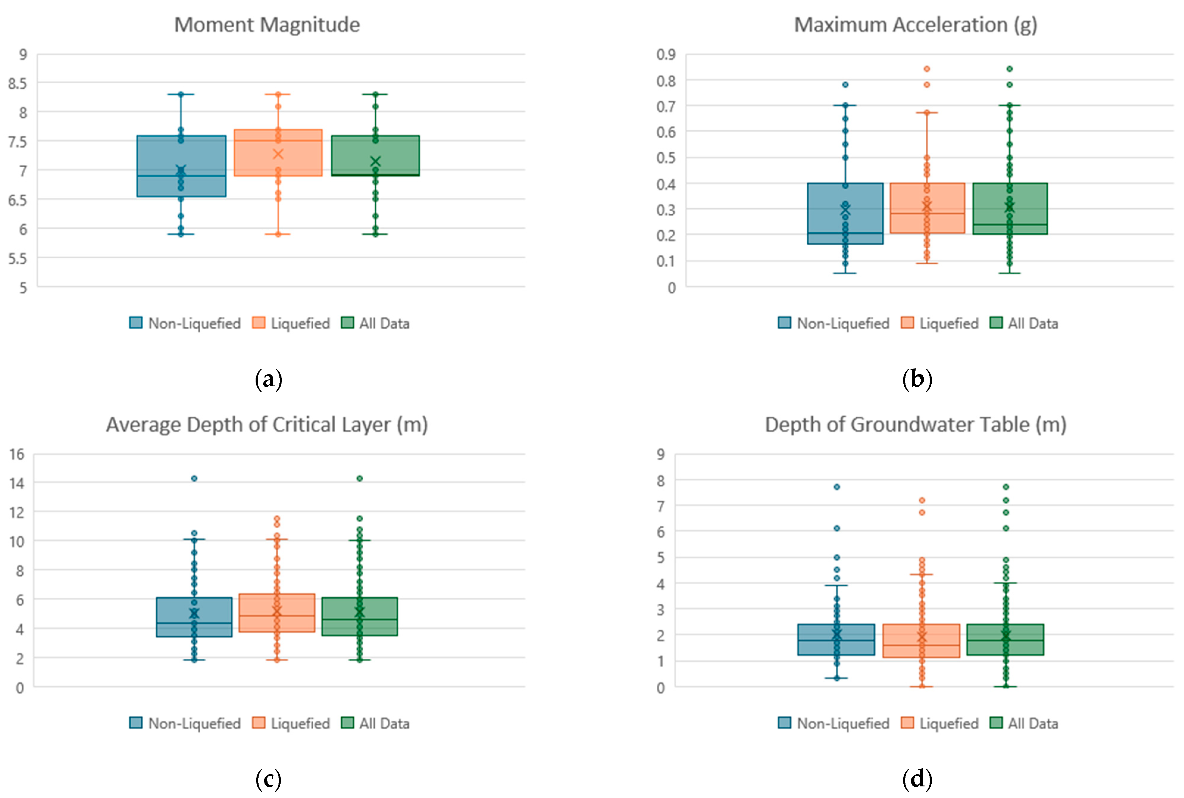
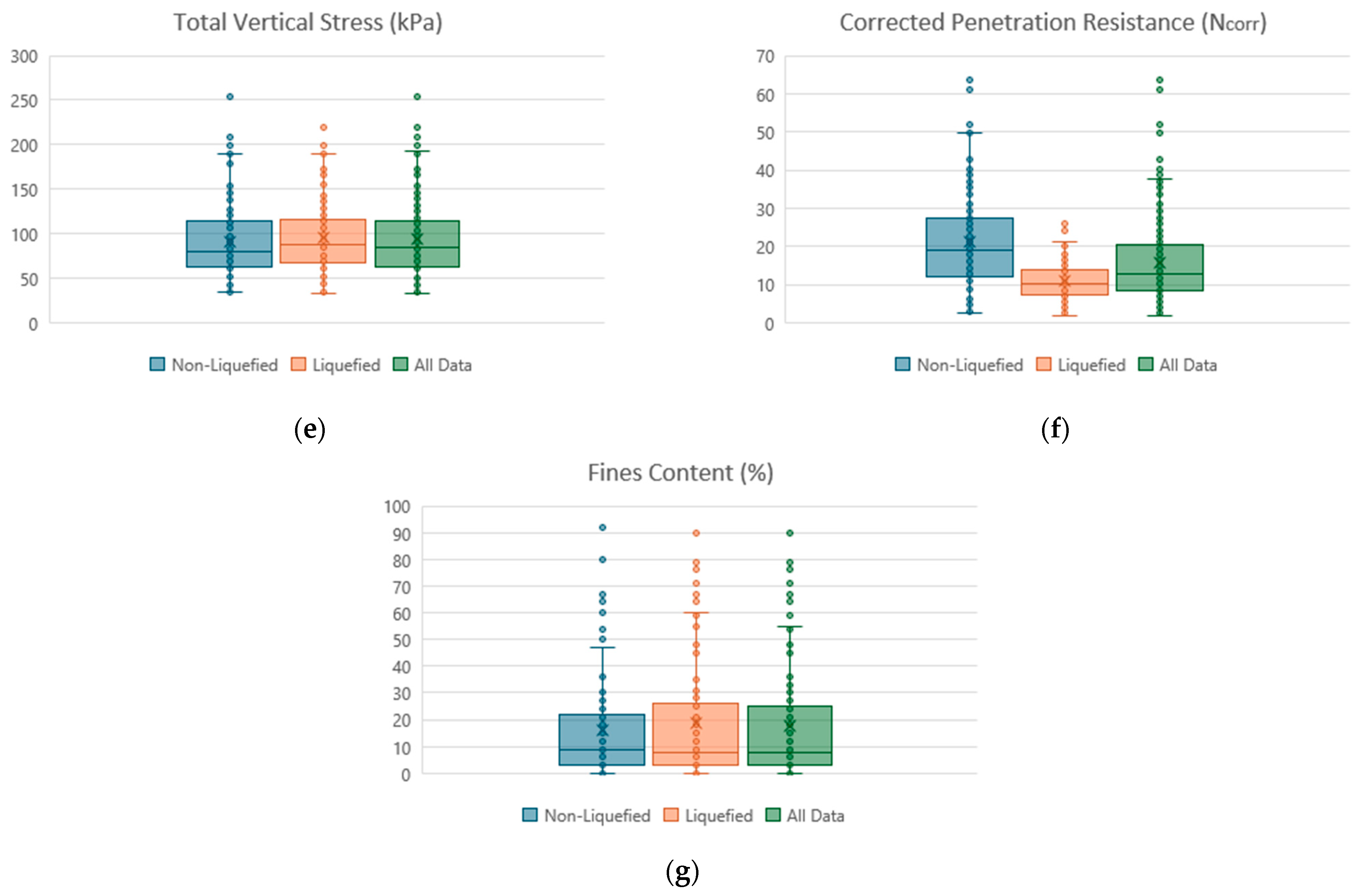
The data distribution of the attributes is also presented in Figure 2. These box and whisker plots are used to discretize and create bins for the conditional attributes. They also serve as the attribute boundaries of the minimum and maximum values for the classification model developed in this study.

2.2. Discretization

Soil liquefaction data are inherently complex, as noted by Maurer and Sanger (2023) [33], and the distributions of some parameters are either lognormal or highly skewed [46,47].

Table 2. Field names, attributes, and discretization of variables.

Attributes	Min–Max Values	Discretization
		Low	Count	High	Count	Outliers	Count
M	5.9–8.3	M < 6.93	109	M ≥ 6.93	142	-	-
amax	0.052–0.84 g	amax < 0.24	113	0.24 ≤ amax < 0.7	132	amax ≥ 0.7	6
Dliq	1.8–14.3 m	Dliq < 4.6	125	4.6 ≤ Dliq < 10.5	120	≥10.5	6
GWT	0–7 m	GWT < 1.8	123	1.8 ≤ GWT < 4	106	≥4	22
σv	32–254 kPa	σv < 86	127	86 ≤ σv < 190	116	≥190	8
Ncorr	1.7–63.7	Ncorr < 13.3	130	13.3 ≤ Ncorr < 39.7	111	≥39.7	10
FC	0–92%	FC < 5	86	5 ≤ FC < 36	128	≥36	37
Liq?	-	Yes		133	No.		118

shows the conditional (input) and the decision (output) attributes used in the modeling process. The conditional attributes include moment magnitude (M), peak horizontal ground acceleration (a_max), average depth of the critical layer (D_liq), depth of the groundwater table (GWT), total vertical stress at the critical depth (σ_v), corrected penetration resistance (N_corr), and the average fines content of the critical layer (FC). The decision attribute has two categorical variables: the “liquefaction” and “no liquefaction” decision classes. Table 2 also includes the discretization and the bins used in the simulation process. Discretization is needed for a rule-based model that is in the IF-THEN format. Moreover, the type of modeling tool, which is rough set-based machine learning, applies to categorical or discrete data. The box and whisker plots were used to discretize the conditional attributes, where the median value separates the “low” bin from the “high”. We adopted median binning in this study to ensure a more robust and representative categorization of the input parameters. This approach aligns with other studies on soil liquefaction that have also utilized the median as a better representation of data parameters [44,47,48]. In skewed distributions, the median is often a more accurate representation of central tendency compared to the mean, as it is less influenced by outliers and skewed data [49]. By using the median, we ensure that our discretization method accurately reflects the underlying data distribution, thereby enhancing the reliability and interpretability of our rule-based model. Moreover, some attributes have outliers, and these outliers were put in the “outlier” bin.

One limitation of ML models includes the scope and range of values used. One study shows the earthquake magnitude threshold value below which liquefaction cannot occur [50]. They suggested that in liquefaction hazard assessments of building sites, magnitude 5.0 be adopted as the minimum earthquake size considered, while magnitudes as low as 4.5 may be appropriate for some other types of infrastructure. Moreover, a study on liquefiable thickness and depth revealed that liquefaction can lead to the failure of piles even at depths greater than 20 m [51]. The present study is limited to liquefaction and non-liquefaction events within the range of values stated in Table 2.

2.3. Rule Induction and Best Model Selection

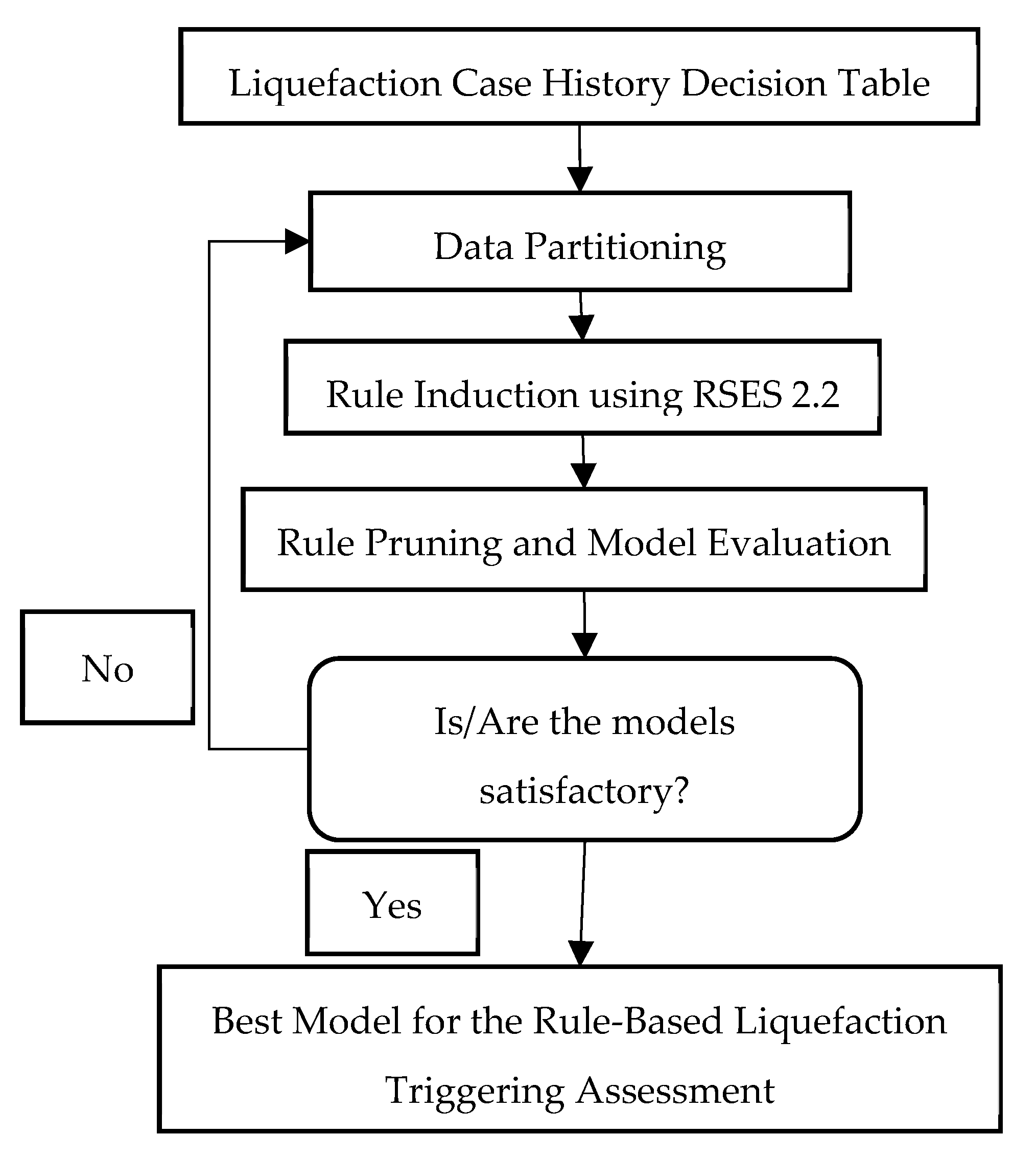
Pawlak (1982) developed RST to address vagueness and uncertainty in knowledge systems [52]. Knowledge is typically represented as a decision table with rows and columns of attributes. Conditions and decisions are two types of attributes in a decision table. Each row on the decision table can be written as IF (conditions)… THEN (decision). Using data from a decision table, an inductive method is used to construct a set of rules. RST has been utilized successfully in a wide range of machine learning applications, including clustering, feature selection, and rule induction. In this work, rule induction was conducted using IF-THEN statements. RSML was used in this study using the rough set exploration system (RSES 2.2) software [53]. Figure 3 shows the flowchart of how RSML was applied in the liquefaction case histories. The first step was to prepare the decision table using the database and Table 2 for the discretization.

Table 3. The decision table used in the study.

No.	M	amax (g)	Dliq (m)	GWT (m)	σv (kPa)	Ncorr	FC (%)	Liq?
1	Low	High	Low	Low	Low	Low	Outlier	Yes
2	Low	High	High	Outlier	High	High	High	No
3	High	High	Low	High	Low	High	Low	Yes
…	…	…	…	...	...	...	...	...
251	High	High	Low	Low	Low	High	Low	Yes

is the decision table showing some of the cases that were already discretized. The next steps included data partitioning, rule induction, rule pruning, and model evaluation. In these steps, trial-and-error was applied to obtain the most satisfactory rule set. The RSES 2.2 software proposes calculation methods (i.e., exhaustive, genetic, covering, and LEM2 algorithms) in rule induction. Rule pruning includes filtering and shortening the rule set.

The shortening procedure adjusts the length of rules by removing or condensing unnecessary or redundant conditions, while retaining their predictive power. This process is guided by a coefficient provided by the user, with a higher coefficient leading to less aggressive shortening and a lower coefficient resulting in a more aggressive shortening of rules. Filtering means that the user can remove rules based on the number of supports or the rules pointing at a particular decision class. For example, the user can remove the rules with only one support. The goal is to simplify and optimize the rules set by removing redundant, irrelevant, or less important rules. Full documentation on RSES 2.2 is available in the manual provided [54].

The basis to determine the best rule set is the F1 score. The rule set that gives the greatest F1 score is considered the best model. The best model is used to classify the reserved test data set.

2.4. Classification

In this study, the standard voting technique was used to determine the final prediction for each case being classified. Figure 4 shows the flowchart of how the standard voting process will be used. The training data set was used to generate the best rule set. Each rule is composed of a set of conditions with the corresponding decision. There are liquefaction and no liquefaction decision classes. The test data set will be classified using these rules. If only one rule is fired up or activated for certain test data, then the prediction of that rule will be adopted. On the other hand, if two or more rules are activated for certain test data, the voting will apply. The decision class with the greater number of supports will take precedence. However, if there is a tie in the voting process, or if there is no rule fired up for particular test data, then the rule set is not able to classify the test data.

The purpose of this classification method is to determine the accuracy of the best model. The proposed rule-based liquefaction triggering model and how it can be used is discussed in detail in Section 4.

2.5. Validation Statistics

To determine the best model or the best rule set, certain validation statistics were used. They included the number of rules, total accuracy, total coverage, F1 score, sensitivity, and the confusion matrix. In this way, one can compare the performances of each rule set regarding their predictions to the test data set. Ultimately, the best rule set was determined by the F1 score statistic. The F1 score has been proven effective in evaluating the performance of a classification model. Equations (1)–(5) show how these metrics were established in terms of the numbers of TP (true positive), TN (true negative), FP (false positive), and FN (false negative).

$$\mathrm{Total}\mathrm{ }Accuracy=\frac{\mathrm{TP}+\mathrm{TN}}{\mathrm{TP}+\mathrm{TN}+\mathrm{FP}+\mathrm{FN}}$$

(1)

$$\mathrm{Recall} \left(\mathrm{Sensitivity}\right)=\frac{\mathrm{TP}}{\mathrm{TP}+\mathrm{FN}}$$

(2)

$$\mathrm{Precision}=\frac{\mathrm{TP}}{\mathrm{TP}+\mathrm{FP}}$$

(3)

$$\mathrm{F}1 \mathrm{Score}=2\ast \frac{\mathrm{Precision}\ast \mathrm{Recall}}{\mathrm{Precision}+\mathrm{Recall}}$$

(4)

$$\mathrm{Total} \mathrm{Coverage}=\frac{\mathrm{Test} \mathrm{objects} \mathrm{recognized} \mathrm{by} \mathrm{the} \mathrm{classifier}}{\mathrm{TN}+\mathrm{TN}+\mathrm{FP}+\mathrm{FN}}$$

(5)

Furthermore, when the best rule set is already selected, the next step is to evaluate each rule contained in the rule set and compare them with each other. In this way, one can understand which rule is the strongest or is the most supported by historical events. Also, this would give insights to decision-makers on how to treat and interpret each rule. The following validation statistics were used: support, strength, certainty factor, and coverage. Supports are observations that adhere to a specific rule. Strength is defined as the ratio of the number of supports to the total observations in the database. The certainty factor is the likelihood that an observation (case history) will be categorized as belonging to a decision class if it exhibits the conditions of a specific rule. The coverage factor indicates the percentage of examples in a decision class that has been categorized because of a specific decision rule.

2.6. Interpretation and Discussion of the Induced Rules

In this part, each rule of the selected best model will be used to create a rule-based liquefaction triggering classification model. Moreover, each rule will be given an interpretation and implication based on the principles of soil mechanics. These interpretations and recommendations will be useful to decision-makers for them to understand the possible scenarios that they may encounter on site given a set of conditions. A proposed classification model was established based on the best model rule set, and the details of how to use the model, example applications, and the advantages and limitations of the model are discussed in the discussion part.

3. Results

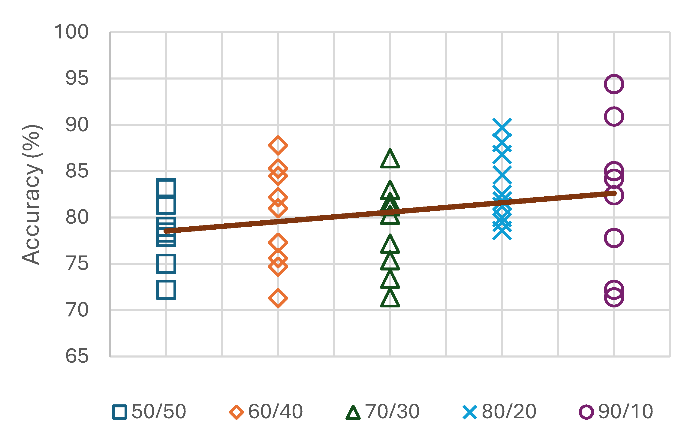
Figure 5 shows the model accuracy of the induced rule sets using their respective independent test sets. Based on the simulation, the 90/10 split (90% training data and 10% test data) proved to be the most effective.

Table 4. Performance of rule sets for 90/10 split.

Statistics of the Rule Set (Calculation Method: Exhaustive Algorithm)
Rule Set	Shortening a	Filtering b	No. of Rules	Total Accuracy (%)	Total Coverage (%)	F1 Score (%)	Sensitivity (%)
1	None	None	187	85	100	86	75
2	0.9	None	136	88	92	89	80
3	0.9	2	53	88	96	90	81
4	0.9	3	32	91	88	93	87
5	0.9	4	21	91	85	92	86

Note: a = shortening coefficient, b = rules with number of supports below these values are removed.

shows the performance of the rule sets developed from the 90/10 split. Rule set 1, without any shortening or filtering, generated 187 rules with 85% accuracy and 100% coverage. This means that the model can predict new data with 85% accuracy, and all the test data received classifications. In contrast, rule set 5, which was shortened once and filtered three times, achieved a total accuracy of 91%, with 85% of new data classified. Additionally, rule set 5 indicates that, with only 21 rules, one can classify liquefaction triggering, reducing its number of rules by almost 9 times compared to rule set 1. It is also noticeable that, as shortening and filtering are applied, rule sets improve in accuracy but decrease in coverage. Lastly, garnering a 93% and 87% F1 score and sensitivity, respectively, rule set 4 emerged as the best set from the induced rule sets. A high F1 score reflects a model’s balanced ability to minimize both false positives and false negatives, while a high sensitivity indicates the model effectively captures most positive instances, minimizing false negatives. Therefore, rule set 4 was chosen as the best rule set.

Table 5. The best model rule set for the liquefied class.

Rules	M	amax (g)	Dliq (m)	GWT (m)	σv (kPa)	Ncorr	FC (%)	Liquefied?	Support
1		High				Low		Yes	50
2	High					Low	Low	Yes	20
3	High			Outlier			High	Yes	7
4	High		Low			Low	High	Yes	22
5	High			Low		Low		Yes	47
6	High	High		Outlier				Yes	5
7	High	Low	High	Low			High	Yes	5
8		High	Low	Low			Outlier	Yes	5
9		High	Low		Low		Outlier	Yes	8
10	High	Low	Low	High				Yes	3
11	Low			Outlier			Outlier	Yes	3
12	High		High	High			Outlier	Yes	4
13	High			High	High		Outlier	Yes	4
14			Low	High		Low	Low	Yes	3
15	Low			High		Low	Low	Yes	4
16					High	Low	Low	Yes	15

and

Table 6. The best model rule set for the non-liquefied class.

Rules	M	amax (g)	Dliq (m)	GWT (m)	σv (kPa)	Ncorr	FC (%)	Liquefied?	Support
17		Low	Low			High		No	24
18		Low			Low	High		No	22
19		Low				High	High	No	13
20						Outlier		No	10
21	Low	Low					High	No	24
22		Low		High		High		No	12
23	High			High		High	High	No	7
24	Low		Low	High		Low	High	No	4
25	Low			High	Low	Low	High	No	4
26	Low	High		Low			Low	No	4
27	Low	Low	High	High				No	3
28	Low	Low		High	High			No	3
29	Low	Low	High				Low	No	3
30	Low	Low			High		Low	No	3
31		Low		High	High		Low	No	4
32	Low	Low				High		No	12

show the rules generated from rule set 4 for the liquefied and non-liquefied cases, respectively. There are 32 rules with each decision class covering 16 rules. Rule-based models are highly transparent because the reasoning behind each decision is explicitly defined by human-readable rules. This makes it easier for users to understand and trust the outputs of the model. For example, rule 1 can be stated as “if there is a high maximum acceleration and low corrected penetration resistance of soil deposits, then liquefaction occurs”. This rule can be easily validated by a geotechnical engineer and can be researched by other non-technical people who want to verify the plausibility of the rule.

From the liquefaction rules, it is generally observed that a high earthquake moment magnitude and low corrected N-values of critical soils tend to trigger liquefaction, especially when coupled with significant cyclic loading from earthquakes, while non-liquefaction rules typically involve low moment magnitudes and low maximum accelerations, combined with high corrected N-values.

However, attention must also be given to other rules that deviate from the common understanding of soil liquefaction. For instance, in liquefaction rule 11, one may question how the combination of low moment magnitude, deep groundwater table depth, and very high fines content of the liquefied layer can trigger liquefaction. The details and interpretation of these rules are discussed in the next section.

The performance statistics for each rule are presented in

Table 7. Validation statistics for best model rule set.

Rule	Support	Strength (%)	Certainty (%)	Coverage (%)
1	50	19.9	94.3	37.6
2	20	8.0	100.0	15.0
3	7	2.8	100.0	5.3
4	22	8.8	95.7	16.5
5	47	18.7	92.2	35.3
6	5	2.0	100.0	3.8
7	5	2.0	100.0	3.8
8	5	2.0	100.0	3.8
9	8	3.2	80.0	6.0
10	3	1.2	75.0	2.3
11	3	1.2	100.0	2.3
12	4	1.6	100.0	3.0
13	4	1.6	100.0	3.0
14	3	1.2	100.0	2.3
15	4	1.6	100.0	3.0
16	15	6.0	93.8	11.3
17	24	9.6	96.0	20.3
18	22	8.8	95.7	18.6
19	13	5.2	100.0	11.0
20	10	4.0	100.0	8.5
21	24	9.6	92.3	20.3
22	12	4.8	100.0	10.2
23	7	2.8	87.5	5.9
24	4	1.6	80.0	3.4
25	4	1.6	80.0	3.4
26	4	1.6	100.0	3.4
27	3	1.2	100.0	2.5
28	3	1.2	100.0	2.5
29	3	1.2	100.0	2.5
30	3	1.2	100.0	2.5
31	4	1.6	100.0	3.4
32	12	4.8	92.3	10.2

. Rule 1 has the highest number of supports, which means that out of all the events in the database, 50 instances support it. Consequently, rule 1 is also the strongest support, with a 19.9% computed strength. For the certainty factor, for those that garnered 100% certainty, it is implied that those rules are deterministic. The certainty factor is the proportion of instances that satisfy both the antecedent (conditions) and the consequent (decision) of the rule, out of all instances that satisfy the antecedent. The certainty factor is also considered the Bayesian probability of each rule. For instance, a certain event that follows rule 1 will have a 94.3% probability that it will liquefy.

Furthermore, the coverage factor of a rule tells us what percentage of examples in a certain class were correctly classified by that rule, showing how well the rule captures instances of that class. For instance, rule 5 covers 35.3% of all cases of liquefaction. In other words, more than one-third of the liquefied cases follow rule 5. These performance statistics present weights to each rule and aid decision-makers in identifying rules that are most effective in capturing patterns in the data.

The performance of the best model with respect to the remaining test data is shown in

Table 8. The performance of the best model against the test data.

No.	M	amax (g)	Dliq (m)	GWT (m)	σv (kPa)	Ncorr	FC (%)	Liquefied?		Activated Rules
								Actual	Model
1	H	L	L	H	L	H	L	No	No	10, 17, 18, 22
2	L	H	H	L	L	L	H	Yes	Yes	1
3	H	H	H	L	H	H	H	Yes	N/A	None
4	L	L	L	H	L	H	H	No	No	17, 18, 19, 21, 22, 32
5	H	H	L	L	L	L	O	Yes	Yes	1, 5, 8, 9
6	H	H	H	H	H	H	H	No	No	23
7	H	L	L	L	L	H	L	No	No	17, 18
8	H	H	H	L	H	H	O	Yes	N/A	None
9	H	H	L	L	L	L	H	Yes	Yes	1, 4, 5
10	L	H	H	H	H	O	L	No	No	20
11	L	L	L	H	L	H	H	No	No	17, 18, 19, 21, 22, 32
12	L	O	L	H	L	L	H	Yes	No	24, 25
13	H	L	L	L	L	L	H	Yes	Yes	4, 5
14	L	O	L	H	L	H	H	No	N/A	None
15	L	H	L	L	L	L	H	Yes	Yes	1
16	H	L	H	H	H	H	H	No	No	19, 22, 23
17	H	L	H	L	H	L	L	Yes	Yes	2, 5, 16
18	H	L	O	H	H	H	L	No	No	18, 22, 31
19	H	H	L	H	L	H	H	Yes	No	23
20	H	L	H	L	O	L	L	Yes	Yes	2, 5
21	H	L	H	H	H	L	O	Yes	Yes	12, 13
22	H	H	H	H	H	L	H	Yes	Yes	1
23	L	L	L	H	L	L	O	No	N/A	None
24	L	H	H	H	H	L	L	Yes	Yes	1, 15, 16
25	L	H	O	O	O	L	H	Yes	Yes	1
26	L	H	H	O	H	L	H	Yes	Yes	1

Note: H = High, L = Low, O = Outlier.

. The standard voting technique is used to classify the test data. In this voting approach, the classification of each test data point is determined based on the rules that are activated for that specific data point. If only one rule is activated for a data point (e.g., events 2, 6, 10, etc.), the decision class associated with that rule is used for classification. For data points where multiple rules are activated within the same decision class (e.g., events 4, 7, 9, etc.), the decision class itself determines the classification.

However, there are cases where a data point may have multiple rules activated from different decision classes simultaneously. In this scenario, the rule with the highest number of supports determines the classification. For example, in event 1, although both liquefaction rule 10 and non-liquefaction rules 17, 18, and 22 are activated, rule 17, having the highest number of supports (24 supports), is chosen to classify event 1. This voting-based approach ensures that the performance of the best model is assessed accurately and objectively based on the activated rules and their associated decision classes for each piece of data. In the test data set classification, out of 26 events, 20 were correctly classified, 2 were classified incorrectly, and 4 could not be classified. Observing the misclassified events, the rules that fired up for events 12 and 19 are rules 23, 24, and 25. These are some of the rules with the lowest certainty factors of less than 90%.

This shows that, while the rule-based model can be improved, it can still be useful as a tool for liquefaction triggering assessment. It has the potential to support decisions, and with better data and a refining of the discretization and rule-creation processes, we might discover more rules that help researchers and decision-makers understand the dynamic behavior of soil, more especially liquefaction.

4. Discussion

In this section, each rule of the chosen best model is interpreted and discussed against the principles of soil mechanics and the available literature. Also, proposed methods for how to use the rule-based liquefaction triggering model developed in this study are discussed. A sample application of the rule-based model is also provided.

4.1. Interpretation of Rules

The following are the interpretations and discussions of the 32 rules from the chosen best model. The rules are grouped into three categories: the top priority, the secondary, and rules governing fine-grained soils. Each discussion includes a statement of the rules in natural language and some explanations based on the literature that support or challenge the generated rules.

4.1.1. Top-Priority Rules

The top-priority rules are those rules that will take precedence when they co-exist with rules from the other decision class. The following are the top-priority rules.

Rule 1. Liquefaction occurs if the maximum acceleration is at least 0.24 g, and the corrected penetration resistance of the critical layer is less than 13.3. Rule 1, which is supported by 50 events, is the most typical scenario of a liquefaction occurrence. With a coverage factor of 37.6%, about one-third of the liquefied cases in the database follow this rule.

Rule 2. If the moment magnitude is 6.93 or higher, and the corrected penetration resistance of the critical layer is less than 13.3, with a fines content of less than 5%, then liquefaction occurs. Rule 2 involves a strong and long-duration earthquake and loose soil with a low corrected N-value and fines content.

Rule 4. If the moment magnitude is at least 6.93, and the critical layer has an average depth of less than 4.6 m, with a corrected penetration resistance of less than 13.3 and a fines content ranging from 5% to less than 36%, then liquefaction occurs. Rule 4 is backed by 20 cases. It shows liquefaction occurrences caused by longer ground shaking, along with low-density sandy soil containing a lot of fines. This can lead to undrained conditions and, ultimately, liquefaction.

Rule 5. If the moment magnitude is 6.93 or higher, the groundwater table is less than 1.8 m deep, and the corrected penetration resistance of the critical layer is less than 13.3, then liquefaction occurs. Rule 5 is backed by 42 cases. Liquefaction can happen due to a stronger and prolonged earthquake combined with a shallow groundwater table, causing loose sandy soils to lose their strength more easily during shaking.

Rule 14. If the groundwater table ranges from 1.8 m to less than 4 m deep, and the critical layer has an average depth of less than 4.6 m, having a corrected penetration resistance of less than 13.3 and a fines content of less than 5%, then liquefaction occurs. Rule 14 involves the liquefaction of loose saturated sands with a small amount of fines content (FC < 5%) near the ground surface (D_liq < 4.6 m).

Rule 15. If the moment magnitude is less than 6.93, the groundwater table ranges from 1.8 m to less than 4 m deep, and the critical layer has a corrected penetration resistance of less than 13.3 and a fines content of less than 5%, then liquefaction occurs. All four cases under rule 15 are from the 1995 Hyogoken-Nambu earthquake.

Rule 16. Liquefaction occurs if the critical layer has a total vertical stress from 86 kPa to less than 190 kPa, the corrected penetration resistance is less than 13.3, and the fines content is less than 5%. These situations entail critical layers (loose, saturated sand) situated 4.6 to 10.5 m underground with very few fines. Rule 16, backed by 13 historical occurrences, saw liquefaction even with a magnitude as low as 6.9 and a maximum acceleration as low as 0.135 g.

Rule 17. No liquefaction occurs if the maximum acceleration is less than 0.24 g, and the critical layer has an average depth of less than 4.6 m and a corrected penetration resistance of at least 13.3. A lower maximum acceleration and relatively high corrected penetration resistance, despite the shallow depth of the critical soil layer, result in the 20 cases supporting rule 17 being non-liquefied.

Rule 18. No liquefaction occurs if the maximum acceleration is less than 0.24 g, and the critical layer has a total vertical stress of less than 86 kPa and a corrected penetration resistance of at least 13.3. Like rule 17, a lower maximum acceleration combined with a relatively high N_corr cannot cause liquefaction, even if the total stress is relatively low.

Rule 19. No liquefaction occurs if the maximum acceleration is less than 0.24 g, and the critical layer has a corrected penetration resistance of at least 13.3, with a fines content of at least 5%. Supported by 10 events, rule 19 states that sands with lots of fine particles and a higher N_corr are less likely to liquefy when subjected to relatively low levels of ground shaking.

Rule 20. No liquefaction occurs if the critical layer has a corrected penetration resistance of 39.7 or higher. Out of the nine supporting events for rule 20, eight were from the 1995 Hyogoken-Nambu (Kobe) earthquake and one was from the 1989 Loma Prieta. The maximum acceleration recorded for these events is as high as 0.7 g, with mostly 0.4 g to 0.6 g. The moment magnitude recorded for these two events was 6.9 for Kobe and 6.93 for Loma Prieta. The other parameters vary. It is a deterministic rule, and it is backed up by the triggering correlation curves developed by other researchers [9,10,11].

Rule 21. No liquefaction occurs if the moment magnitude is lower than 6.93, the maximum acceleration is less than 0.24 g, and the fines content of the critical layer ranges from 5% to less than 36%. Supported by 22 events, this rule suggests that liquefaction is improbable. This conclusion could be due to the insufficient magnitude of ground shaking as depicted by the lower magnitude and maximum acceleration. However, given the broad range of discretization bins of some parameters, the blank condition for the N_corr, and a certainty factor of 92.3%, there remains a possibility of liquefaction in some events. It is advisable to complement this rule with other liquefaction assessment tools.

Rule 22. No liquefaction occurs if the maximum acceleration is less than 0.24 g, the groundwater table is 1.8 m or deeper, and the critical layer has a corrected penetration resistance of at least 13.3. Low-magnitude acceleration, combined with a relatively deep groundwater table and higher N_corr, results in a lower chance of liquefaction.

Rule 32. No liquefaction occurs if the moment magnitude is lower than 6.93, the maximum acceleration is less than 0.24 g, and the critical layer has a corrected penetration resistance of at least 13.3.

4.1.2. Secondary Rules

Secondary rules are supporting rules that can be overruled by the top-priority rules if they co-exist with each other on a particular site. They also represent the rare and curious cases of liquefied or non-liquefied events that ensure the model is comprehensive and covers a wider range of scenarios. Nevertheless, these rules can still be used to classify liquefaction triggering potential when they are the only rules that will activate in a particular site or soil layer. The following are the interpretations of the secondary rules.

Rule 3. If the moment magnitude is at least 6.93, the groundwater table is located 4 m or deeper, and the fines content of the critical layer ranges from 5% to less than 36%, then liquefaction occurs. Rule 3, supported by seven events, has a certainty factor of 100%. Meaning, it is a deterministic rule.

Rule 6. If the moment magnitude is 6.93 or higher, the maximum acceleration is at least 0.24 g, and the groundwater table is at least 4 m deep, then liquefaction occurs. This rule is rather odd or confusing because there is no accounting for other geotechnical-related parameters. However, looking back to the database, events that support this rule have an average depth of 6–7 m, an N_corr of 9.4–20.9, and a fines content of 5–32%. This rule predominantly represents sand layers located at relatively deeper layers that liquefied due to the combination of high values of earthquake magnitude and maximum acceleration.

Rule 7. If the moment magnitude is 6.93 or higher, the maximum acceleration is less than 0.24 g, the groundwater table is less than 1.8 m deep, and the average depth of the critical layer ranges from 4.6 m to less than 10.5 m, with a fines content ranging from 5% to less than 36%, then liquefaction occurs. Rule 7 is liquefiable with five supports. These cases revealed that a combination of a strong and long-duration earthquake and a lower maximum acceleration (less than 0.24 g) can still generate liquefaction. The number of uniform cycles, which is a parameter highly correlated with the earthquake magnitude, is also a governing factor in this rule. However, according to the database, for the liquefaction to occur in this case, the corrected penetration resistance value should be in the “Low” bin.

Rule 10. If the moment magnitude is 6.93 or higher, the maximum acceleration is less than 0.24 g, the groundwater table ranges from 1.8 m to less than 4 m deep, and the critical layer depth is less than 4.6 m, then liquefaction occurs. Cases governed by rule 10 can only liquefy if the N_corr value is in the “low” range (N_corr < 13.3). Otherwise, liquefaction is less likely to occur.

Rule 23. If the moment magnitude is 6.93 or higher, the groundwater table ranges from 1.8 m to less than 4 m deep, and the critical layer has a corrected penetration resistance value of at least 13.3, with a fines content ranging from 5% to less than 36%, then no liquefaction occurs. This rule represents some events where a strong and long-duration earthquake did not make a relatively dense, saturated soil liquefy.

Rule 24. If the moment magnitude is lower than 6.93, the groundwater table is 1.8 m or deeper, and the critical layer has an average depth of less than 4.6 m and has a corrected penetration resistance value of less than 13.3, with a fines content that ranges from 5% to less than 36%, then no liquefaction occurs. Rule 24 says a low-magnitude earthquake will not liquefy loose soil, but with a higher maximum acceleration, as rule 1 suggests, liquefaction can happen.

Rule 25. If the moment magnitude is lower than 6.93, the groundwater table is 1.8 m or deeper, and the critical layer has a total vertical stress of less than 86 kPa and a corrected penetration resistance value of less than 13.3, with a fines content ranging from 5% to less than 36%, then no liquefaction occurs.

Rule 26. If the moment magnitude is lower than 6.93, the maximum acceleration is less than 0.7 g, the groundwater table is less than 1.8 m deep, and the critical layer has a fines content of less than 5%, then no liquefaction occurs. Rule 26 indicates no liquefaction despite a high maximum acceleration. However, in the database, the events for rule 26 have N_corr values that fall within the higher range (i.e., 31.6–49.7).

Rule 27. If the moment magnitude is lower than 6.93, the maximum acceleration is less than 0.24 g, the groundwater table is 1.8 m or deeper, and the critical layer has an average depth of 4.6 m or deeper, then no liquefaction occurs.

Rule 28. If the moment magnitude is lower than 6.93, the maximum acceleration is less than 0.24 g, the groundwater table is 1.8 m or deeper, and the critical layer has a total vertical stress of at least 86 kPa, then no liquefaction occurs.

Rule 29. If the moment magnitude is lower than 6.93, the maximum acceleration is less than 0.24 g, and the critical layer has an average depth of 4.6 m or deeper, with a fines content of less than 5%, then no liquefaction occurs.

Rule 30. If the moment magnitude is lower than 6.93, the maximum acceleration is less than 0.24 g, and the critical layer has a total vertical stress of at least 86 kPa, with a fines content of less than 5%, then no liquefaction occurs.

Rule 31. If the maximum acceleration is less than 0.24 g, the groundwater table is 1.8 m or deeper, and the critical layer has a total vertical stress of at least 86 kPa, with a fines content of less than 5%, then no liquefaction occurs.

4.1.3. Rules Governing Fine-Grained Soils

This study found that the liquefaction or softening of fine-grained soils was evident in some of the rules it generated. Specifically, five rules showed instances where silty sands or fine-grained soils exhibited liquefaction or liquefaction-like effects during the site investigation. The following rules outline the conditions under which liquefaction occurs in fine-grained soils.

Rule 8. If the maximum acceleration is at least 0.24 g, the groundwater table is less than 1.8 m, and the critical layer has an average depth of less than 4.6 m, with a fines content of 36% or more, then liquefaction occurs. Rule 8 deals with silt liquefaction and/or the softening of fine-grained soils. This rule is supported by four sites from the 1999 Kocaeli earthquake. According to a team of researchers that investigated these sites in Adapazari, Turkey, damage caused by the earthquake was due in part to liquefaction and ground softening [55]. Moreover, they concluded that liquefaction did occur in Adapazari, but the softening of fine-grained soils due to cyclic mobility and the working of buildings into the softened soils under these buildings was more prevalent [55]. Thus, when the rule-based model proposed in this study is used and rule 8 is activated, the occurrence of both the liquefaction and softening of soil, if not cyclic softening alone, is likely to occur.

Rule 9. If the maximum acceleration is at least 0.24 g, and the critical layer has an average depth of less than 4.6 m and total vertical stress of less than 86 kPa, with a fines content of 36% or more, then liquefaction occurs. Rule 9, like rule 8, represents the liquefaction and/or cyclic softening of fine-grained soils. Most of the representative sites that supported rule 9 are from Adapazari, Turkey, during the 1999 Kocaeli earthquake.

Rule 11. Liquefaction occurs if the moment magnitude is less than 6.93, the groundwater table is 4 m or deeper, and the fines content of the critical layer is 36% or higher. Rule 11 describes situations where loose fine-grained layers are saturated and shaken by a higher maximum acceleration. Although the N_corr and a_max are not present in the conditions, looking at the database, the three representative events show N_corr values of 3.9–13.1 while the a_max ranges from 0.45 g to 0.84 g. The investigation of the two sites in the 1971 San Fernando earthquake that support rule 11 revealed that the main sources of liquefaction were loose sandy silt and silty sand deposits sandwiched by denser layers of soil [56]. Three influencing factors towards liquefaction during the 1971 San Fernando earthquake were grain size, groundwater table, and peak acceleration [56].

Rule 12. If the moment magnitude is 6.93 or higher, the groundwater table ranges from 1.8 m to less than 4 m deep, and the average depth of the critical layer ranges from 4.6 m to less than 10.5 m, with a fines content of 36% or higher, then liquefaction occurs. Rule 12 deals with deep loose soil deposits (4.6 m to 10.5 m underground). The presence of a significant percentage of fines in the soil prevents drainage during long-duration ground shaking, triggered by a high moment magnitude which leads to strength reduction.

Rule 13. If the moment magnitude is 6.93 or higher, the groundwater table ranges from 1.8 m to less than 4 m deep, and the total vertical stress is from 86 kPa to less than 190 kPa, with a fines content of 36% or higher, then liquefaction occurs. The situation in rule 13 is quite like rule 12, where a higher fines content and longer ground shaking cause liquefaction.

Rules 8, 9, 11, 12, and 13 all deal with the liquefaction of silty sands or fine-grained soils. Depending on mineral content, soil behavior under cyclic loading is different. In a comprehensive report dealing with fine-grained soils, the potential for liquefaction or cyclic failure depends on two types of soil behavior: “sand-like” or “clay-like” fine-grained soils [20]. For practical purposes, Boulanger and Idriss (2004) recommended that fine-grained soils with a PI < 7 indicate a “sand-like” response (i.e., susceptible to liquefaction), and soils with a PI ≥ 7 indicate a “clay-like” response [20]. Moreover, Bray and Sancio (2006) observed that the liquefaction of some fine-grained soils is characterized by “cyclic mobility with limited flow deformation” [19]. They argued that excess pore pressure on low-plasticity silts during undrained cyclic loading can lead to a loss in effective stress, but, upon shearing, the dilative tendency of silts can produce a dramatic increase in stiffness. They also described this phenomenon as liquefaction because of the presence of ground surface manifestations like soil ejecta, ground settlement, cracking, building settlement, etc. [19]. Arguably, it is the amount and type of clay minerals in the soil that best indicate liquefaction susceptibility, not the amount of “clay-size” particles [19]. For practical purposes, whenever any of these rules governing fined-grained soils are activated during the liquefaction assessment, it is recommended to include a cyclic failure/cyclic softening assessment with the critical layer involved. Nevertheless, it is preferred to perform laboratory tests to assess the liquefaction susceptibility and strain potential of these soils, given the loading conditions existing in the field.

4.2. Application of the Rule-Based Liquefaction Triggering Classification Model

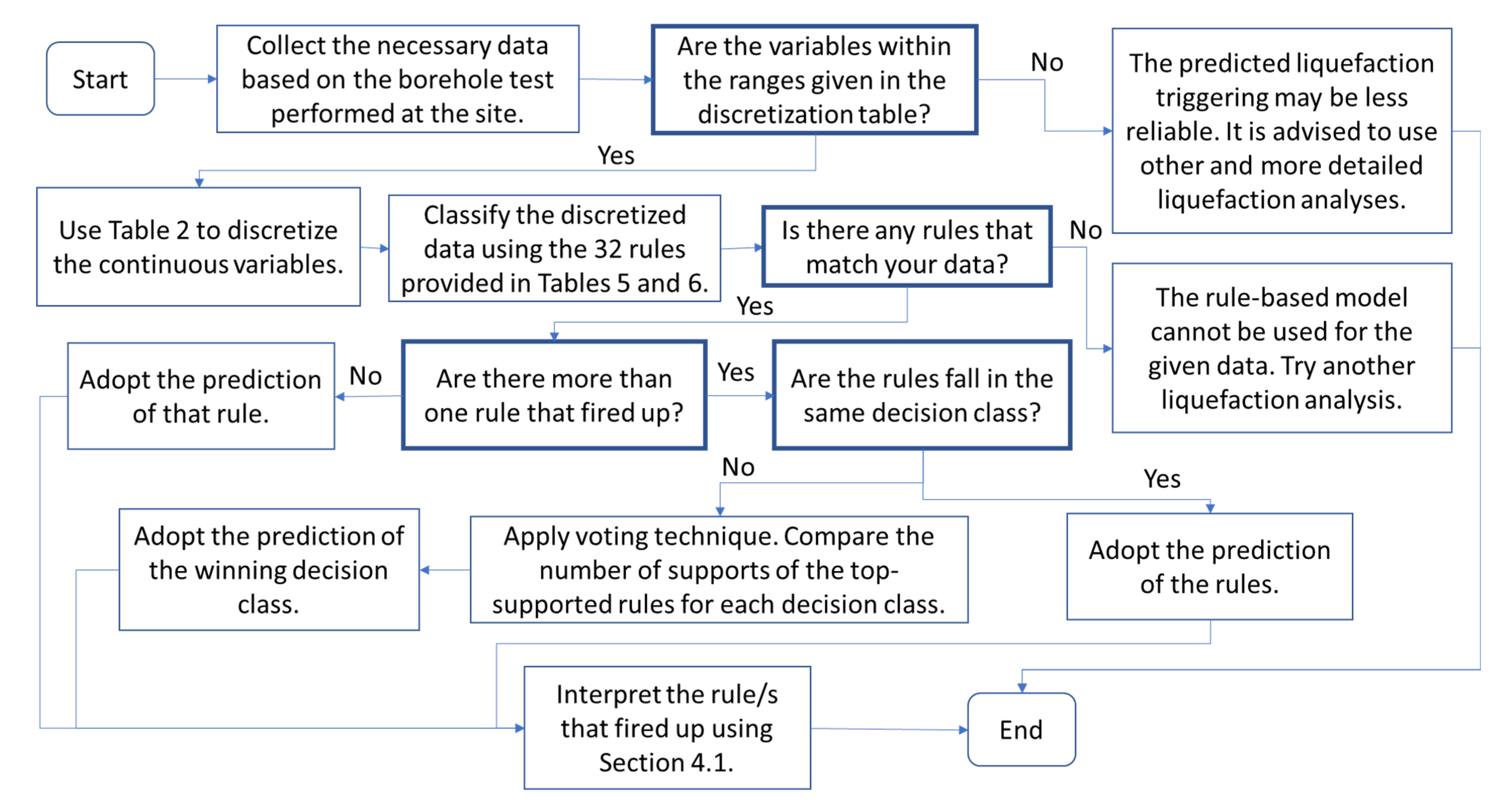
Figure 6 shows the flowchart of how to use the developed rule-based liquefaction triggering classification model. It starts with the collection of the data needed and the discretization of the continuous data. After discretizing the data, prepare the decision table and check the rules in Table 5 and Table 6 that are activated with the given set of conditions. Classify the given conditions using the standard voting technique discussed earlier. The rule with the highest number of supporting cases will prevail. When there are two or more conflicting decision classes that arise, having the same number of supports, choose the more conservative decision class, i.e., liquefaction will occur. The rule-based model is not recommended in cases when the given data are not within the ranges of values in the discretization table, and it is not applicable when no rule is activated during the classification. It is recommended to use other methods for such cases. It should be noted that the user must check all the rules that may be activated before determining the classification of a site. This step ensures that all potential patterns from the historical database are considered.

In their 2022 study, Demir and Sahin reported that their robust ML algorithms for liquefaction prediction achieved accuracies and F-measure values between 83 and 96% [28]. Conversely, Maurer and Sanger (2023) found that tier-2 state-of-practice (SOP) liquefaction models typically have efficiencies ranging from 70 to 85% [33]. According to them, tier-2 SOP models utilize in situ geotechnical data and mechanistic principles to predict a liquefaction response for one-dimensional profiles. The performance statistics of the rule-based model proposed in this study are comparable to those of other published ML models. Although directly comparing the accuracy and efficiency of ML models with SOP or conventional models is challenging, a practical comparison using actual borehole data was provided to assess the performance of the rule-based model.

A sample application of the rule-based liquefaction triggering classification model is presented in Figure 7. Borehole data from a site in Manila City, the Philippines, were used. The moment magnitude used is 6 and the maximum ground acceleration is 0.3 g. The groundwater table depth is located 1.3 m below the ground surface. Using the simplified procedures [11], the factor of safety for each layer was computed for the critical layers (i.e., the color-shaded regions) susceptible to liquefaction as shown in Figure 7b. On the other hand, the assessment of the rule-based model revealed the layers that will potentially liquefy, given the conditions. Rule 1, which is the highest supported rule, was activated in the 2–7 m and 8–10.5 m layers. In addition, rules 8 and 9 were also activated in the lean clay layer at 2–3 m. This implies that there is a potential for the softening of this soft, low-plasticity clay layer during ground shaking. Apparently, when the factor of safety is less than or slightly above 1.00, certain rules are activated. On the other hand, the SC layer at a depth of 12 m, which recorded a factor of safety of 1.55, activated no rules. The outcomes of the simplified procedures correspond with those of the rule-based model.

In summary, while the simplified semi-empirical procedures provide a broad overview of liquefaction susceptibility through triggering curves based on a summary of case histories, the rule-based model offers a more detailed and context-specific assessment by considering individual site conditions and historical events. Using the same parameters as the simplified procedures provides a consistent baseline for comparison; however, the true value of the rule-based model lies in its potential to incorporate additional insights, adapt to evolving knowledge, and provide transparent decision-making frameworks. Most importantly, with its adaptability and flexibility, the rule-based model allows for updates or modifications to the rules based on new information, changes in understanding, or site-specific considerations, which can enhance the model’s accuracy and relevance over time.

4.3. Novelty and Significance of the Proposed Model

The following points highlight the novelty, significance, and usefulness of the proposed methods, rules, model, and results from this study.

1. Comparing the proposed model with the semi-empirical stress-based model (e.g., Boulanger and Idriss [11]) indicates that it aligns well with current industry standards, thereby boosting its credibility.

2. The methods for model development are clearly explained and can be replicated by others. To identify the best rule set, the study should select the set with the highest statistical parameters. In this context, cross-validation and other standard statistical validation processes are not necessary, as the focus is on deriving the optimal rule set directly from the data using rough set-based machine learning. However, the testing of independent validation data, shortening, and filtering were employed to ensure quality performance and avoid overfitting.

3. While some rules reflect established geotechnical knowledge, this study adds novelty by uncovering patterns in liquefaction and non-liquefaction sites from case histories. For instance, rule 11 uniquely addresses fine-grained soils, identifying a specific combination of factors that lead to liquefaction: lower earthquake magnitude, deeper critical soil depths, high ground acceleration, and increased fines content. This multifactorial approach highlights the complexity of liquefaction and provides nuanced insights, helping engineers assess risks in fine-grained soils and identify vulnerable sites that might be overlooked using traditional criteria.

4. This rule-based model does not provide a liquefaction triggering classification only but also a context-specific approach to liquefaction assessment which is not provided in most of the state-of-practice methods and most AI models. The state-of-practice simplified procedure on liquefaction triggering serves as a summary of liquefaction case histories by providing a generalized relationship between CSR and CRR. In contrast, by analyzing the characteristics of historical liquefaction events and identifying patterns in the data, the rule-based model offers a more tailored and context-specific approach to liquefaction assessment.

5. For practical applications, the developed rules are designed to provide clear and actionable guidelines for assessing liquefaction hazards. These rules can be integrated into geotechnical practice to enhance the efficiency and reliability of decision-making processes. It can also be practically useful, particularly in time-sensitive situations or in regions with a limited access to experienced engineers. These rules provide practical guidance for disaster risk management, without the need for complex formulas or models, relying instead on easily interpretable criteria.

6. Aside from the provided statistical validation for the model itself, each rule in the rule-based model has its own strength and certainty factors that can be a guide to users. This empirical backing enhances credibility not only with the model but also with the rules. Backing by a substantial number of cases suggests that a rule has been observed consistently in real-world scenarios.

7. This rule-based model was designed to be user-friendly and less complex to use and comprehend. Other AI models, as emphasized by Maurer and Sanger (2023), are complex, unapproachable, and are not provided by their developers [33].

5. Conclusions

This study introduced a rule-based liquefaction triggering classification model developed through rule induction using rough set-based machine learning. After a series of processes, a set of 32 rules was chosen as the best model. Very satisfactory validation metrics were obtained for the best model rule set, with a total accuracy of 91% and an F1 score of 93% when tested against the independent validation data set. The generated 32 rules were grouped into three: top priority, secondary, and rules governing fine-grained soils. These rules provide context-specific liquefaction scenarios under various conditions. Some of the worth-noting conditions are as follows.

1. Rule 11, a rule governing fine-grained soils, highlights that a lower earthquake magnitude and deeper critical soil depths can lead to liquefaction, when combined with high ground acceleration and increased fines content.

2. Rule 7 indicates that even a maximum acceleration as low as 0.16 g can induce liquefaction in critical soil layers at depths of up to 6.5 m. This is influenced by factors such as a high earthquake magnitude, shallow groundwater tables, and increased fines content, which collectively contribute to undrained conditions.

3. Fifteen historical cases show that loose, saturated sand with a low fines content liquefied at depths between 4.6 m to less than 10.5 m. Moreover, liquefaction occurred when either earthquake magnitude or maximum acceleration was high. For instance, during the 1976 Guatemala earthquake, even a low maximum acceleration of 0.135 g, combined with a high moment magnitude of 7.5, led to liquefaction, supporting rule 16, which is a top-priority rule.

4. Rule 20, a top-priority rule and a one-condition rule, states that when the corrected penetration resistance value reaches 39.7 or higher, liquefaction will not occur. While the highest recorded N_corr that liquefied in the database is 25.9, it falls within the “high” bin in the discretization table. However, once the N_corr reaches the outlier bin, liquefaction will never occur regardless of other conditions. Nonetheless, the question lingers as to what maximum threshold of N_corr will trigger liquefaction.

5. In high-magnitude earthquakes (M ≥ 6.93), liquefaction was absent due to higher N_corr values (13.3 to less than 39.7), yielding an 87.5% certainty of no liquefaction according to rule 23. However, under increased maximum ground acceleration, instances such as the 1993 Kushiro-Oki event, with a recorded maximum acceleration of 0.47 g, contradicted this expectation by experiencing liquefaction, validating rule 23.

6. Rules 24 and 25 show that even though a site is clearly prone to liquefaction (N_corr < 13.3), it may not liquefy if the seismic conditions are low. For instance, during the 1987 Superstition Hills earthquake, a site with a N_corr of 2.9 did not liquefy, despite a moment magnitude of 6.54 and a maximum acceleration of 0.15 g.

7. Rule 32, a top-priority rule and one backed by 12 events, reflects sites with low seismic parameters. The average and median N_corr values in these cases are 17.5 and 15.2, respectively, with a median moment magnitude and maximum acceleration of 6.5 and 0.16 g. Thus, for sites expecting seismic loading within these ranges, maintaining a corrected penetration resistance value of at least 17.5 is enough to prevent liquefaction.

In terms of attribute selection, the moment magnitude and maximum horizontal acceleration have been selected as the key demand attributes. These parameters are crucial for capturing the essential aspects of seismic demand, including the intensity and duration of shaking. While these two parameters provided a sufficient representation of the demand part in the rule-based model, future development could benefit from incorporating other energy dissipation parameters.

This study also offers a clear flowchart for utilizing the rule-based model, demonstrated through practical examples using a borehole log. Results from the state-of-practice simplified procedures for liquefaction triggering align well with the proposed rule-based model. The application of the rule-based liquefaction triggering classification model can provide a more contextual liquefaction assessment, in addition to other semi-empirical or numerical procedures.

Furthermore, the rule-based liquefaction triggering assessment model offers advantages such as interpretability and transparency, while also handling noisy and missing data. One of the most important advantages of a rule-based model over other machine learning models is its legibility and simplicity. Other models provide numerical values (i.e., a factor of safety, probability of liquefaction, dissipated energy, etc.) in a liquefaction assessment. The rule-based model, on the other hand, allows an understanding of which attributes and combinations are important in determining which sites are liquefiable and which are not. However, it faces challenges like discretization and attribute dependency, which can be mitigated through careful data management and rule validation.

Topics for further study include the expansion of the ranges of values in the database and the exploration and validation of some rules with curious conditions using laboratory or field experiments. Additionally, liquefaction-like phenomena have been observed in some cases involving fine-grained soils; it would be necessary to include in future developments some fine-grained soil characteristics, such as Atterberg limits. Furthermore, applying the methods developed in this study to address other geotechnical engineering challenges such as lateral spreading, sand boils, landslides, energy-based liquefaction assessment, and slope stability analysis is ongoing.

References

1. Ishihara, K. Stability of Natural Deposits during Earthquakes. In Proceedings of the 11th International Conference on Soil Mechanics and Foundation Engineering, San Francisco, CA, USA, 12–16 August 1985; AA Balkema Publishers: Rotterdam, The Netherlands, 1985; Volume 1, pp. 321–376. [Google Scholar]
2. Day, R.W. Geotechnical Earthquake Engineering Handbook; McGraw-Hill: New York, NY, USA, 2002; ISBN 978-0-07-137782-9. [Google Scholar]
3. Daniell, J.E.; Schaefer, A.M.; Wenzel, F. Losses Associated with Secondary Effects in Earthquakes. Front. Built Environ. 2017, 3, 30. [Google Scholar] [CrossRef]
4. Kramer, S.L. Geotechnical Earthquake Engineering; Prentice-Hall International Series in Civil Engineering and Engineering Mechanics; Prentice Hall: Upper Saddle River, NJ, USA, 1996; ISBN 978-0-13-374943-4. [Google Scholar]
5. Seed, H.B.; Lee, K.L. Liquefaction of Saturated Sands During Cyclic Loading. J. Soil Mech. Found. Div. 1966, 92, 105–134. [Google Scholar] [CrossRef]
6. Seed, H.B.; Idriss, I.M. Simplified Procedure for Evaluating Soil Liquefaction Potential. J. Soil Mech. Found. Div. 1971, 97, 1249–1273. [Google Scholar] [CrossRef]
7. Robertson, P.K.; Wride, C. (Fear) Evaluating Cyclic Liquefaction Potential Using the Cone Penetration Test. Can. Geotech. J. 1998, 35, 442–459. [Google Scholar] [CrossRef]
8. Andrus, R.D.; Stokoe, K.H., II. Liquefaction Resistance of Soils from Shear-Wave Velocity. J. Geotech. Geoenviron. Eng. 2000, 126, 1015–1025. [Google Scholar] [CrossRef]
9. Youd, T.L.; Idriss, I.M.; Andrus, R.D.; Arango, I.; Castro, G.; Christian, J.T.; Dobry, R.; Finn, W.D.L.; Harder, L.F.; Hynes, M.E.; et al. Liquefaction Resistance of Soils: Summary Report from the 1996 NCEER and 1998 NCEER/NSF Workshops on Evaluation of Liquefaction Resistance of Soils. J. Geotech. Geoenviron. Eng. 2001, 127, 817–833. [Google Scholar] [CrossRef]
10. Cetin, K.O.; Seed, R.B.; Der Kiureghian, A.; Tokimatsu, K.; Harder, L.F.; Kayen, R.E.; Moss, R.E.S. Standard Penetration Test-Based Probabilistic and Deterministic Assessment of Seismic Soil Liquefaction Potential. J. Geotech. Geoenviron. Eng. 2004, 130, 1314–1340. [Google Scholar] [CrossRef]
11. Boulanger, R.W.; Idriss, I.M. CPT and SPT Based Liquefaction Triggering Procedures; Center for Geotechnical Modeling Department of Civil and Environmental Engineering University of California: Davis, CA, USA, 2014. [Google Scholar]
12. Green, R.A.; Bommer, J.J.; Rodriguez-Marek, A.; Maurer, B.W.; Stafford, P.J.; Edwards, B.; Kruiver, P.P.; De Lange, G.; Van Elk, J. Addressing Limitations in Existing ‘Simplified’ Liquefaction Triggering Evaluation Procedures: Application to Induced Seismicity in the Groningen Gas Field. Bull. Earthq. Eng. 2019, 17, 4539–4557. [Google Scholar] [CrossRef]
13. Upadhyaya, S.; Green, R.A.; Rodriguez-Marek, A.; Maurer, B.W. True Liquefaction Triggering Curve. J. Geotech. Geoenviron. Eng. 2023, 149, 04023005. [Google Scholar] [CrossRef]
14. Dobry, R.; Ladd, R.S. Discussion of “Soil Liquefaction and Cyclic Mobility Evaluation for Level Ground during Earthquakes and Liquefaction Potential: Science Versus Practice”. J. Geotech. Eng. Div. 1980, 106, 720–724. [Google Scholar] [CrossRef]
15. Dobry, R.; Ladd, R.S.; Yokel, F.Y.; Chung, R.M.; Powell, D. Prediction of Pore Water Pressure Buildup and Liquefaction of Sands during Earthquakes by the Cyclic Strain Method.; National Bureau of Standards: Gaithersburg, MD, USA, 1982. [Google Scholar]
16. Rodriguez-Arriaga, E.; Green, R.A. Assessment of the Cyclic Strain Approach for Evaluating Liquefaction Triggering. Soil Dyn. Earthq. Eng. 2018, 113, 202–214. [Google Scholar] [CrossRef]
17. Berrill, J.B.; Davis, R.O. Energy Dissipation and Seismic Liquefaction of Sands: Revised Model. Soils Found. 1985, 25, 106–118. [Google Scholar] [CrossRef] [PubMed]
18. Ulmer, K.J.; Green, R.A.; Rodriguez-Marek, A.; Mitchell, J.K. Energy-Based Liquefaction Triggering Model. J. Geotech. Geoenviron. Eng. 2023, 149, 04023105. [Google Scholar] [CrossRef]
19. Bray, J.D.; Sancio, R.B. Assessment of the Liquefaction Susceptibility of Fine-Grained Soils. J. Geotech. Geoenviron. Eng. 2006, 132, 1165–1177. [Google Scholar] [CrossRef]
20. Boulanger, R.W.; Idriss, I.M. Evaluating the Potential for Liquefaction or Cyclic Failure of Silts and Clays; Center for Geotechnical Modeling Department of Civil & Environmental Engineering University of California: Davis, CA, USA, 2004. [Google Scholar]
21. Goh, A.T.C. Seismic Liquefaction Potential Assessed by Neural Networks. J. Geotech. Eng. 1994, 120, 1467–1480. [Google Scholar] [CrossRef]
22. Abbaszadeh Shahri, A. Assessment and Prediction of Liquefaction Potential Using Different Artificial Neural Network Models: A Case Study. Geotech. Geol. Eng. 2016, 34, 807–815. [Google Scholar] [CrossRef]
23. Fahim, A.K.F.; Rahman, M.Z.; Hossain, M.S.; Kamal, A.S.M.M. Liquefaction Resistance Evaluation of Soils Using Artificial Neural Network for Dhaka City, Bangladesh. Nat. Hazards 2022, 113, 933–963. [Google Scholar] [CrossRef]
24. Pal, M. Support Vector Machines-Based Modelling of Seismic Liquefaction Potential. Int. J. Numer. Anal. Methods Geomech. 2006, 30, 983–996. [Google Scholar] [CrossRef]
25. Kohestani, V.R.; Hassanlourad, M.; Ardakani, A. Evaluation of Liquefaction Potential Based on CPT Data Using Random Forest. Nat. Hazards 2015, 79, 1079–1089. [Google Scholar] [CrossRef]
26. Gandomi, A.H.; Fridline, M.M.; Roke, D.A. Decision Tree Approach for Soil Liquefaction Assessment. Sci. World J. 2013, 2013, 346285. [Google Scholar] [CrossRef]
27. Chen, Z.; Li, H.; Goh, A.T.C.; Wu, C.; Zhang, W. Soil Liquefaction Assessment Using Soft Computing Approaches Based on Capacity Energy Concept. Geosciences 2020, 10, 330. [Google Scholar] [CrossRef]
28. Demir, S.; Şahin, E.K. Liquefaction Prediction with Robust Machine Learning Algorithms (SVM, RF, and XGBoost) Supported by Genetic Algorithm-Based Feature Selection and Parameter Optimization from the Perspective of Data Processing. Environ. Earth Sci. 2022, 81, 459. [Google Scholar] [CrossRef]
29. Hanandeh, S.M.; Al-Bodour, W.A.; Hajij, M.M. A Comparative Study of Soil Liquefaction Assessment Using Machine Learning Models. Geotech. Geol. Eng. 2022, 40, 4721–4734. [Google Scholar] [CrossRef]
30. Rateria, G.; Maurer, B.W. Evaluation and Updating of Ishihara’s (1985) Model for Liquefaction Surface Expression, with Insights from Machine and Deep Learning. Soils Found. 2022, 62, 101131. [Google Scholar] [CrossRef]
31. Galupino, J.; Dungca, J. Estimating Liquefaction Susceptibility Using Machine Learning Algorithms with a Case of Metro Manila, Philippines. Appl. Sci. 2023, 13, 6549. [Google Scholar] [CrossRef]
32. Karimai, K.; Liu, W.; Maruyama, Y. Prediction and Factor Analysis of Liquefaction Ground Subsidence Based on Machine-Learning Techniques. Appl. Sci. 2024, 14, 2713. [Google Scholar] [CrossRef]
33. Maurer, B.W.; Sanger, M.D. Why “AI” Models for Predicting Soil Liquefaction Have Been Ignored, plus Some That Shouldn’t Be. Earthq. Spectra 2023, 39, 1883–1910. [Google Scholar] [CrossRef]
34. Maass, W.; Parsons, J.; Purao, S.; Storey, V.C.; Woo, C. Data-Driven Meets Theory-Driven Research in the Era of Big Data: Opportunities and Challenges for Information Systems Research. J. Assoc. Inf. Syst. 2018, 19, 1253–1273. [Google Scholar] [CrossRef]
35. Kökçam, A.H.; Erden, C.; Demir, A.S.; Kurnaz, T.F. Bibliometric Analysis of Artificial Intelligence Techniques for Predicting Soil Liquefaction: Insights and MCDM Evaluation. Nat. Hazards 2024. [Google Scholar] [CrossRef]
36. Rudin, C.; Chen, C.; Chen, Z.; Huang, H.; Semenova, L.; Zhong, C. Interpretable Machine Learning: Fundamental Principles and 10 Grand Challenges. Stat. Surv. 2022, 16, 1–85. [Google Scholar] [CrossRef]
37. Aviso, K.B.; Janairo, J.I.B.; Promentilla, M.A.B.; Tan, R.R. Prediction of CO2 Storage Site Integrity with Rough Set-Based Machine Learning. Clean Technol. Environ. Policy 2019, 21, 1655–1664. [Google Scholar] [CrossRef]
38. Gue, I.H.V.; Lopez, N.S.A.; Chiu, A.S.F.; Ubando, A.T.; Tan, R.R. Predicting Waste Management System Performance from City and Country Attributes. J. Clean. Prod. 2022, 366, 132951. [Google Scholar] [CrossRef]
39. Chang, S.-H.; Wan, S. Discrete Rough Set Analysis of Two Different Soil-Behavior-Induced Landslides in National Shei-Pa Park, Taiwan. Geosci. Front. 2015, 6, 807–816. [Google Scholar] [CrossRef]
40. Liu, L.; Dou, Y.; Qiao, J. Evaluation Method of Highway Plant Slope Based on Rough Set Theory and Analytic Hierarchy Process: A Case Study in Taihang Mountain, Hebei, China. Mathematics 2022, 10, 1264. [Google Scholar] [CrossRef]
41. Arabani, M.; Pirouz, M. Liquefaction Prediction Using Rough Set Theory. Sci. Iran. 2019, 26, 779–788. [Google Scholar] [CrossRef]
42. Liu, N.P.; Wang, H.T.; Yuan, Z.G. Evaluation Indexes of Sand Liquefaction Analysed by Rough Set. Adv. Mater. Res. 2011, 243–249, 3087–3091. [Google Scholar] [CrossRef]
43. Baykasoğlu, A.; Çevik, A.; Özbakır, L.; Kulluk, S. Generating Prediction Rules for Liquefaction through Data Mining. Expert Syst. Appl. 2009, 36, 12491–12499. [Google Scholar] [CrossRef]
44. Torres, E.S. An interpretable machine learning approach in understanding lateral spreading case histories. Int. J. Geomate 2024, 26, 110–117. [Google Scholar] [CrossRef]
45. Committee on Soil Dynamics of the Geotechnical Engineering Division. Definition of Terms Related to Liquefaction. J. Geotech. Eng. Div. 1978, 104, 1197–1200. [Google Scholar] [CrossRef]
46. Zhu, J.; Baise, L.G.; Thompson, E.M. An Updated Geospatial Liquefaction Model for Global Application. Bull. Seismol. Soc. Am. 2017, 107, 1365–1385. [Google Scholar] [CrossRef]
47. Ntritsos, N.; Cubrinovski, M. Ground-Motion Effects on Liquefaction Response. Soil Dyn. Earthq. Eng. 2024, 177, 108392. [Google Scholar] [CrossRef]
48. Idriss, I.M.; Boulanger, R.W. SPT-Based Liquefaction Triggering Procedures; Center for Geotechnical Modeling Department of Civil and Environmental Engineering University of California: Davis, CA, USA, 2010. [Google Scholar]
49. Greenberg, B. Excel Manual for Moore, McCabe, and Craig’s Introduction to the Practice of Statistics, 6th ed.; W.H. Freeman and Company: New York, NY, USA, 2009. [Google Scholar]
50. Green, R.A.; Bommer, J.J. What Is the Smallest Earthquake Magnitude That Needs to Be Considered in Assessing Liquefaction Hazard? Earthq. Spectra 2019, 35, 1441–1464. [Google Scholar] [CrossRef]
51. Ari, A.; Demir, S.; Özener, P. Examining the Role of Liquefiable Layer Thickness and Depth on the Seismic Lateral Response of Piles through Numerical Analyses. Int. J. Geomech. 2023, 23, 04023047. [Google Scholar] [CrossRef]
52. Pawlak, Z. Rough Sets. Int. J. Comput. Inf. Sci. 1982, 11, 341–356. [Google Scholar] [CrossRef]
53. Bazan, J.G.; Szczuka, M. The Rough Set Exploration System. In Transactions on Rough Sets III.; Lecture Notes in Computer Science; Peters, J.F., Skowron, A., Eds.; Springer: Berlin/Heidelberg, Germany, 2005; Volume 3400, pp. 37–56. ISBN 978-3-540-25998-5. [Google Scholar]
54. Bazan, J.G.; Szczuka, M. RSES 2.2 User’s Guide; Warsaw University: Warsaw, Poland, 2005. [Google Scholar]
55. Bray, J.D.; Sancio, R.B.; Durgunoglu, T.; Onalp, A.; Youd, T.L.; Stewart, J.P.; Seed, R.B.; Cetin, O.K.; Bol, E.; Baturay, M.B.; et al. Subsurface Characterization at Ground Failure Sites in Adapazari, Turkey. J. Geotech. Geoenviron. Eng. 2004, 130, 673–685. [Google Scholar] [CrossRef]
56. Bennett, M.J. Liquefaction Analysis of the 1971 Ground Failure at the San Fernando Valley Juvenile Hall, California. Environ. Eng. Geosci. 1989, 26, 209–226. [Google Scholar] [CrossRef]
Figure 1. The general flow of processes.
Geosciences 14 00156 g001
Figure 2. Box plots of the conditional attributes (input parameters) with respect to the decision attribute (output parameter): (a) moment magnitude, (b) maximum horizontal acceleration, (c) average depth of critical layer, (d) depth of groundwater table, (e) total vertical stress, (f) corrected penetration resistance, and (g) fines content.
Geosciences 14 00156 g002aGeosciences 14 00156 g002b
Figure 3. The application of rough set machine learning and the selection of the best model in the liquefaction case history database.
Geosciences 14 00156 g003
Figure 4. Classification process in determining accuracy of chosen best model using standard voting technique.
Geosciences 14 00156 g004
Figure 5. The model accuracy of the induced rule sets using their respective independent test sets.
Geosciences 14 00156 g005
Figure 6. A flowchart of how to use the developed rule-based liquefaction triggering classification model.
Geosciences 14 00156 g006
Figure 7. A liquefaction assessment of a sample borehole showing (a) the fines content plot, (b) Ncorr plot, (c) the factor of safety plot using Boulanger and Idriss (2014) procedures [11], and (d) the activated rules using the liquefaction triggering rule-based model developed in this study.
Geosciences 14 00156 g007