Abstract
The correct selection of the value of p is a complex and iterative procedure that requires experience in the interpretation of the obtained interpolated maps. Inverse Distance Weighting is a method applied to the porosities of the K and L hydrocarbon reservoirs discovered in the Neogene (Lower Pontian) subsurface sandstones in northern Croatia (Pannonian Basin System). They represent small and large data samples. Also, a standard statistical analysis of the data was made, followed by a qualitative–quantitative analysis of the maps, based on the selection of different values for the power distance exponent (p-value) for the K and L reservoir maps. According to the qualitative analysis, for a small data set, the p-value could be set at 1 or 2, giving the optimal result, while for a large data set, a p value of 3 or 4 could be applied. For quantitative analysis, in the case of a small data set, p = 2 is recommended, resulting in a root mean square error value of 0.03458, a mean absolute error of 0.02013 and a median absolute deviation of 0.00546. In contrast, a p-value of 3 or 4 is selected as appropriate for a large data set, with root mean square errors of 0.02435 and 0.02437, mean square errors of 0.01582 and 0.01509 and median absolute deviations 0.00896 and 0.00444. Eventually for a small data set, it is recommended to use a p-value of 2, and for a large data set, a p-value of 3 or 4.
1. Introduction
Inverse Distance Weighting (IDW) is an interpolation method that is widely used in geosciences. The method is applied to small and large input data sets. Various authors have applied IDW during different mappings of variables: mapping the distribution of a nickel deposit [1], geomorphology [2], estimated copper, molybdenum, gold and silver with respect to lithogeochemical data in the Kahang porphyry deposit in Central Iran [3], modeling of ionospheric time delay [4], spatial distribution maps of groundwater [5], spatial distribution of groundwater pollution maps [6], mapping of gold deposits based on drilled shallow wells [7], soil salinity mapping in the Mirzaabad District, Syrdarya Province [8], and the estimation of tin resources [9].
It is obvious that IDW is a widely used interpolation method in different geosciences for spatial 2D visualization, and it is often compared with other interpolations like the Kriging techniques, Nearest Neighborhood or Moving Average. Its popularity arises from the simple algorithm, where the weighting of measured values comes from their distances, but users also can vary such weights with a power exponent. So, some control is retained but calculation is simple and fast for very large data sets (hundreds of points). The decades-long use of IDW and comparison with other methods is not the goal of this paper; however, some examples from Croatia are useful to mention to lead readers to knowledge of the “main” interpolation “competitors” of IDW, their advantages and disadvantages. So, ref. [10] showed the spatial variability of soil organic matter content in Eastern Croatia assessed using different interpolation methods, namely, IDW, Ordinary Kriging and Bayesian Kriging. Only the Kriging techniques are main competitors of IDW, assuming that spatial variability could be better described with such an algorithm, which is not always true (especially for data sets with less than 20 points, or for more numerous but highly clustered data sets).
The hydrocarbon reservoirs in the Northern Croatia Miocene subsurface sandstones are just such borderline examples, where the numbers of the data are at the limits for creating a detailed spatial model using a variogram and continuing with the Kriging techniques, as opposed to choosing a simpler mathematical method like IDW and decreasing the error of faulty complex modeling. Sometimes, for the larger fields, the Kriging techniques can be successfully applied for smaller data sets, e.g., the depth data for 18 wells on the Upper Pannonian/Lower Pontian border (i.e., E-log marker Z’) in the Šandrovac Field [11] interpolated with the Universal Kriging. However, this is mostly an exception, not the standard rule.
Obviously, reliable subsurface mapping is crucial for all hydrocarbon reservoirs in the Sava Depression, and northern Croatia in general, especial in the current late production stage, when the maximum predicted recovery has been almost reached in all fields. As the porosity is one of the major reservoir variables, such mapping must be (re)made as reliable as possible, especially when not all wells have reliable log measurements and core analysis. So, the available data sets are often much smaller than the total number of wells drilled in the field’s structure. Also, porosity mapping in the Croatian hydrocarbon reservoirs was done using other algorithms and interpretation methods, mostly successfully reaching the possible visualization of reservoir models. Further, ref. [12] compared the sweetness seismic attribute and (also) porosity and porosity-thickness maps (obtained by Ordinary Kriging) in the Sava Depression. Also, ref. [13] used stochastic simulation for mapping reservoir geological variables (porosity, thickness, depth) in the Sava Depression (18–23 wells available for the mapped structure). The authors recommended that sequential Gaussian simulation can be used for structural variations, and Indicator Kriging and sequential indicator simulation for the mapping of depositional environment morphology.
Application of the IDW algorithm is dependent on its simple equations. The estimated value of the IDW variable is calculated using the following formula: [14,15,16]:
where:
| ZIDW | estimated value; |
| d1 … dn | distance between estimated value and known value 1 … n; |
| p | power distance exponent; |
| z1 … zn | known values at locations 1 … n. |
The mapping results are greatly influenced by the power distance exponent (p); this is clear because it represents the exponent of a value that is inversely reciprocal to the known “hard” data, as can be seen from Formula (1). This is why it is important to choose p correctly so that the obtained interpolated maps are usable and mathematically based. Both the size (small or large) and the nature of the input data set should be considered when choosing p. The wrong selection of p can lead to asymmetry in the resulting interpolation maps, which should be avoided. In this paper, the selection of p will be analyzed considering the quantitative (sample size, cross-validation) and qualitative (visual inspection and interpretation) aspects of the obtained interpolation maps.
2. Materials and Methods
For the analysis of the value of p, it is necessary to take into account the material and applied methods. The material data were contained in the values of the porosity of the reservoirs K and L. In addition to the previously described IDW, the coefficient of interquartile deviation, root mean square error, mean absolute error and median absolute deviation calculations were applied for the analysis.
2.1. Coefficient of Interquartile Deviation
Coefficient of interquartile deviation (VQ) is a measure of the incomplete dispersion of a data set, and is defined as [17,18]:
where:
| VQ | coefficient of interquartile deviation; |
| Q1 | the value of the lower (first) quartile of the sample; |
| Q3 | the value of the upper (third) quartile of the sample. |
The value of the coefficient is between 0 and 1, and the condition for its application is that all input data are positive values (>0). The dispersion of the data is smaller the closer VQ is to 0, and relatively larger the closer VQ is to 1.
2.2. Root Mean Square Error (RMSE)
Cross-validation is a numerical value obtained as the difference of the square of the measured and estimated data values. Mean square error is calculated according to [19,20]:
where:
| MSE | mean square error value; |
| n | number of known values; |
| SV | measured value of point “i”; |
| P | estimated value of point “i”; |
| i | ith point. |
It quantitatively expresses the quality of the interpolation map; the lower the RMSE value is, the higher the acceptability of the interpolated map. During the interpolation process, while changing various parameters, RMSE is a corrective for interpolation maps because it reduces the space for gross errors. The root mean square error value is calculated according to [21,22]:
where:
| RMSE | root mean square error value; |
| MSE | mean square error value. |
The fact that the RMSE is based on the root function of the error itself means that larger errors will contribute less in absolute terms. This is very important when analyzing a large input data set.
2.3. Mean Absolute Error (MAE)
Mean absolute error is a measure of error calculated as the difference between the measured and estimated sample values. The formula for calculating MAE is [23,24]:
where:
| MAE | mean absolute error; |
| n | number of known values; |
| SV | measured value of point “i”; |
| P | estimated value of point “i”; |
| i | ith point. |
As can be seen from Expression (5), the MAE represents a comparison between the “firm” data and the estimated data. The MAE method is sensitive to extreme values within the input data set.
2.4. Median Absolute Deviation (MAD)
Median absolute deviation is the median value of the difference between the estimated value and the value of the “solid” data. MAD is calculated according to the following equation [25,26]:
where:
| MAD | median absolute deviation; |
| SV | measured value of point “i”; |
| P | estimated value of point “i”; |
| i | ith point. |
3. Geographic Location, Geological Settings and Raw Data of Analyzed Reservoirs
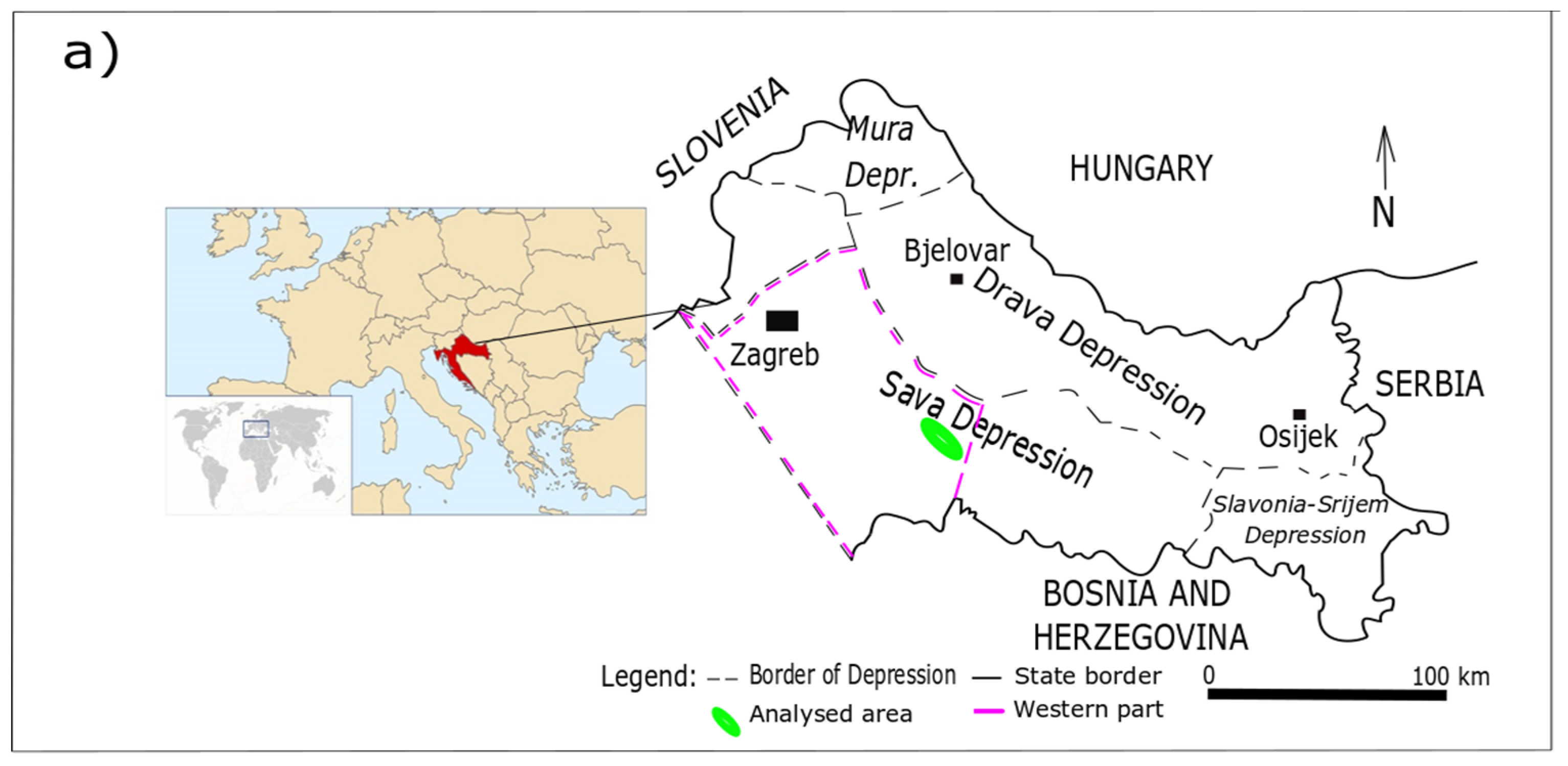
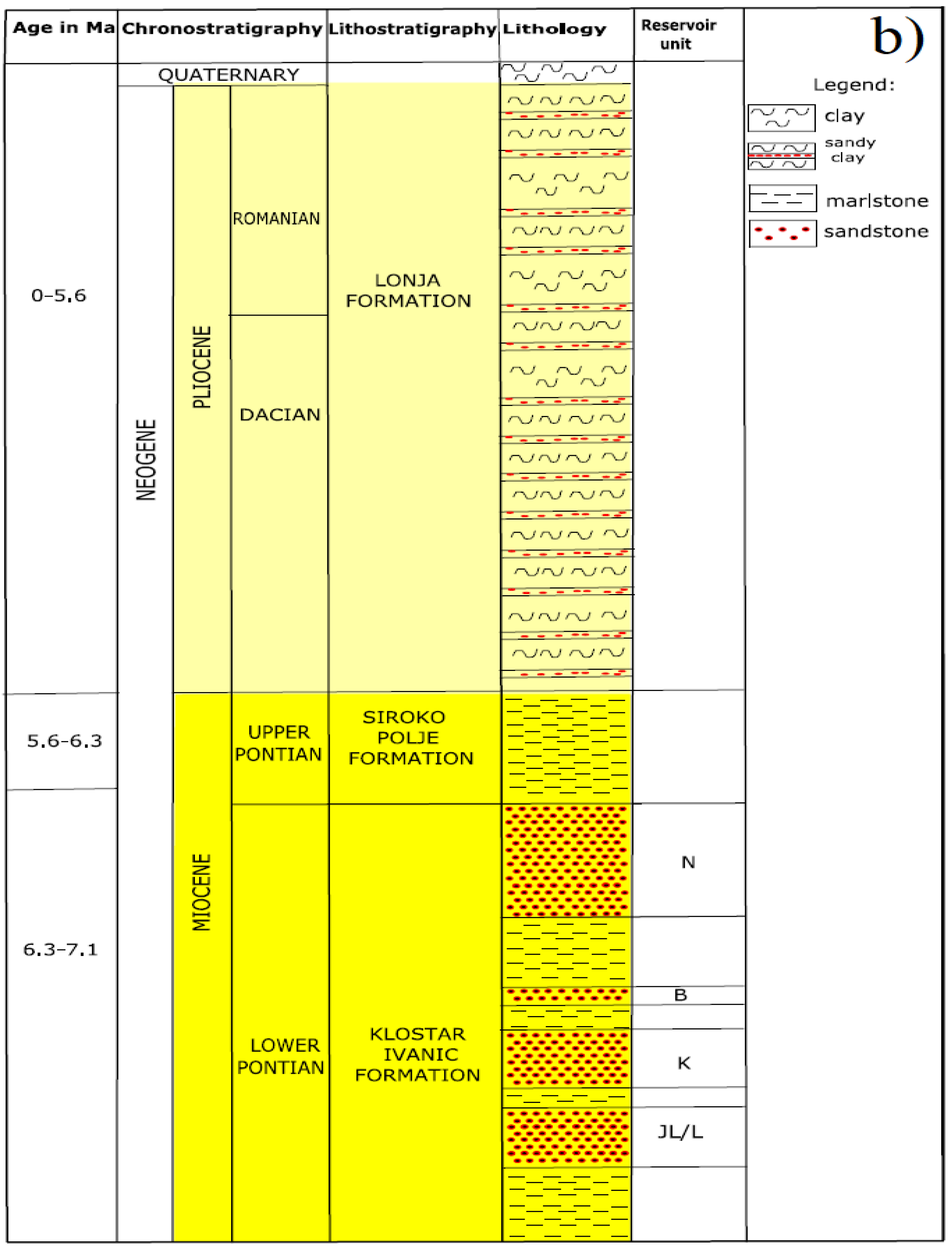
Research fields “A” and “B” were located within the Sava Depression, in the Croatian part of the Pannonian Basin System (CPBS) (see Figure 1a). Sediments filling the Sava Depression started already in the Early Neogene (Otnangian), and in this study, Lower Pontian reservoir rocks (reservoirs K and L) belonging to the Kloštar-Ivanić Formation were analyzed (see geological column in Figure 1b).

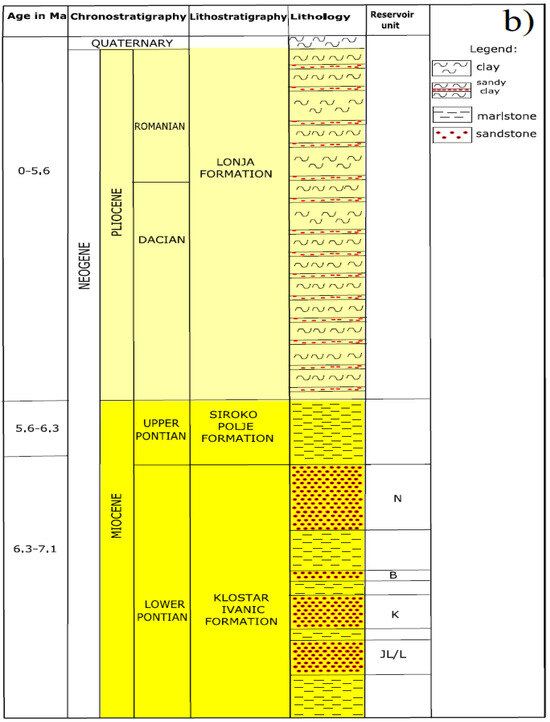
Figure 1.
Geographical position (a) and geological column (b) of research fields A and B within the Sava Depression, modified after [27,28].
These are mainly well-sorted arenitic sandstones, becoming fine-grained and loose toward the top of the Široko Polje Formation, and intercalated with marl intervals. Reservoir rocks are well-lithified sandstones, with an average thickness of 20–150 m. Isolator rocks are gray to gray-brown marls, moderately lithified, appearing in 30–150 m thick intervals between sandstones.
The Lower Pontian sediments (also known informally by their older name, the Abichi deposits, after the characteristic fossil shell Paradacna abichi) extended across the entire Sava Depression, but in the westernmost part can be referred to as the Kloštar-Ivanić Marls (as a lateral equivalent of the Kloštar-Ivanić Formation), or locally as the Brezine or Graberje Marl. The analyzed sandstones (as part of the Poljana Sandstones) are the result of periodically activated turbidites and are deposited in the deepest part of the depression. The rest had been filled with marls, occasionally silty ones.
The most important petrophysical parameter during reservoir analysis is porosity. Data on the porosity of the deposits K and L were obtained by analyzing cores from a well or by interpreting logging diagrams. Particularly, the porosity data were calculated by interpretation of resistivity, density and neutron logs. For the K reservoir, data from 3 wells (25, 120 and 168), and for the L reservoir 10 wells (2, 5, 57, 60, 62, 68, 73, 85, 87 and 145), were also available from lab analysis, but were not used for this mapping [29]. The reason lay in the values from the lab analyses, which were somewhat higher than those from the logs, so a conservative approach to reservoir quality favored using the lower, i.e., log-interpreted/calculated, values. The permeability (not used here) was solely derived from laboratory analysis of cores.
The porosity value for the K reservoir was obtained from 19 wells (average depth 975 m), while for the L reservoir it was obtained from 25 wells (average depth 1370 m), and these were considered “solid” data, i.e., the original data during various analyses. Basic statistical data on the porosity of the reservoirs K and L are shown in Table 1. It is obvious that the quality and resolution of the measuring devices and the transformation of indirect signals into values had significant limitations, especially in reservoir K, where numerous wells have the same average porosity value as for sandstone. However, this is a common limitation that must be overcome using the most appropriate interpolation algorithm, and handled using the same values as for the same kinds of “clusters”, even if they are not located in the same neighborhood.

Table 1.
Porosity data for K and L reservoirs [30]. The X and Y are geographical positions of wells fitting the Gauss–Krueger coordinate system, zone 6.
4. Results and Discussion
The choice of reservoirs was made considering the sizes of the input data sets. The sizes of the input data sets were taken from the authors of [31], according to which reservoir K belongs to a small data set, while reservoir L belongs to a large data set. The values of the coefficient of interquartile deviation for the K and L reservoirs are presented in Table 2.

Table 2.
Values of the coefficient of interquartile deviation for the K and L reservoirs.
According to Table 2, the VQ value for the K reservoir is 0.013, while for the L reservoir it is 0.054. According to these values, the porosity of these reservoirs is significantly dispersed. This was to be expected due to the nature of the input data and the method used to obtain them. Due to the high economic cost of obtaining data, the input data set is in most cases very dispersed. Precisely because of the high dispersion of the data, the IDW method was applied for mapping reservoirs K and L.
4.1. Qualitative Analysis of Maps
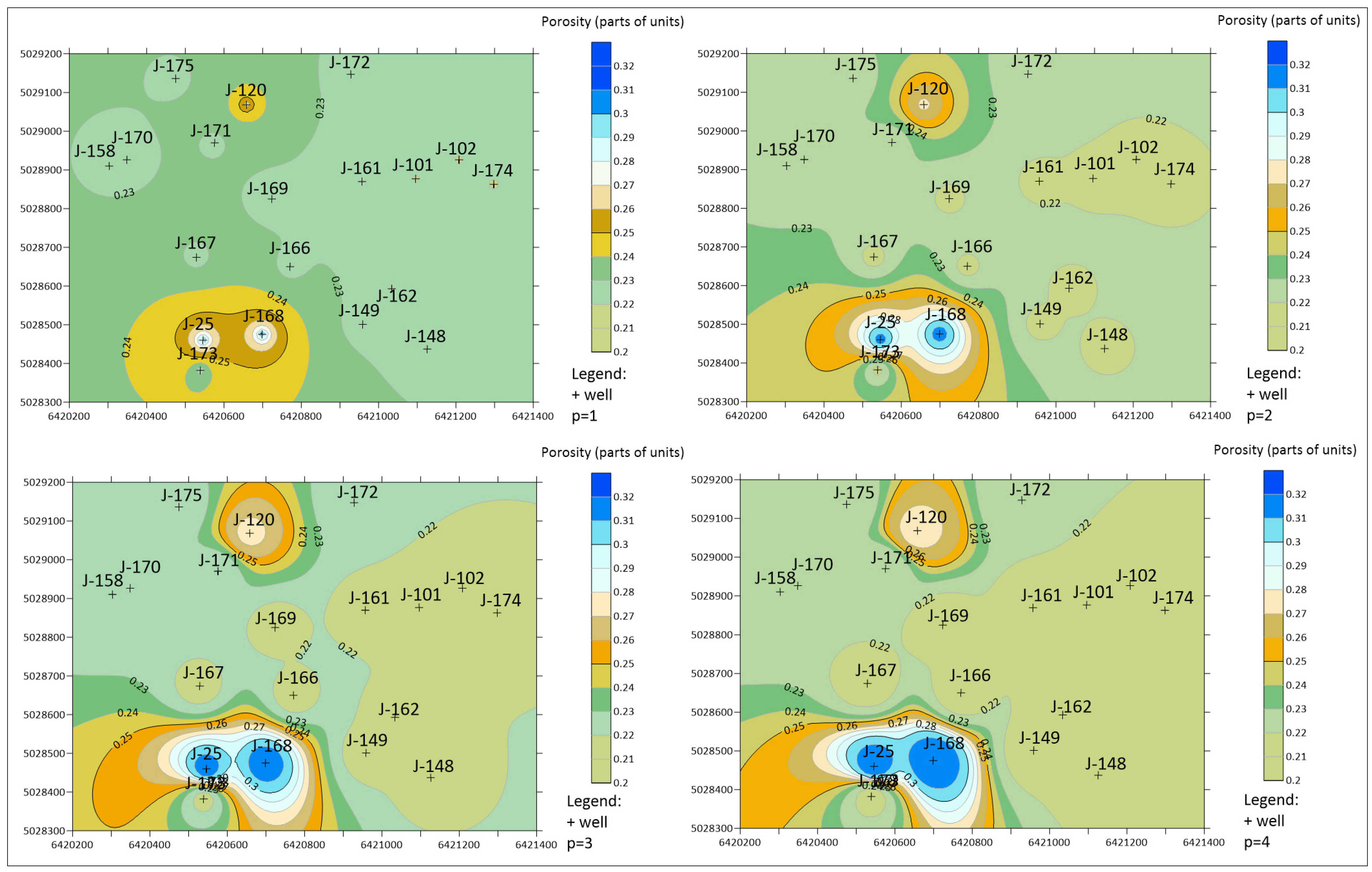
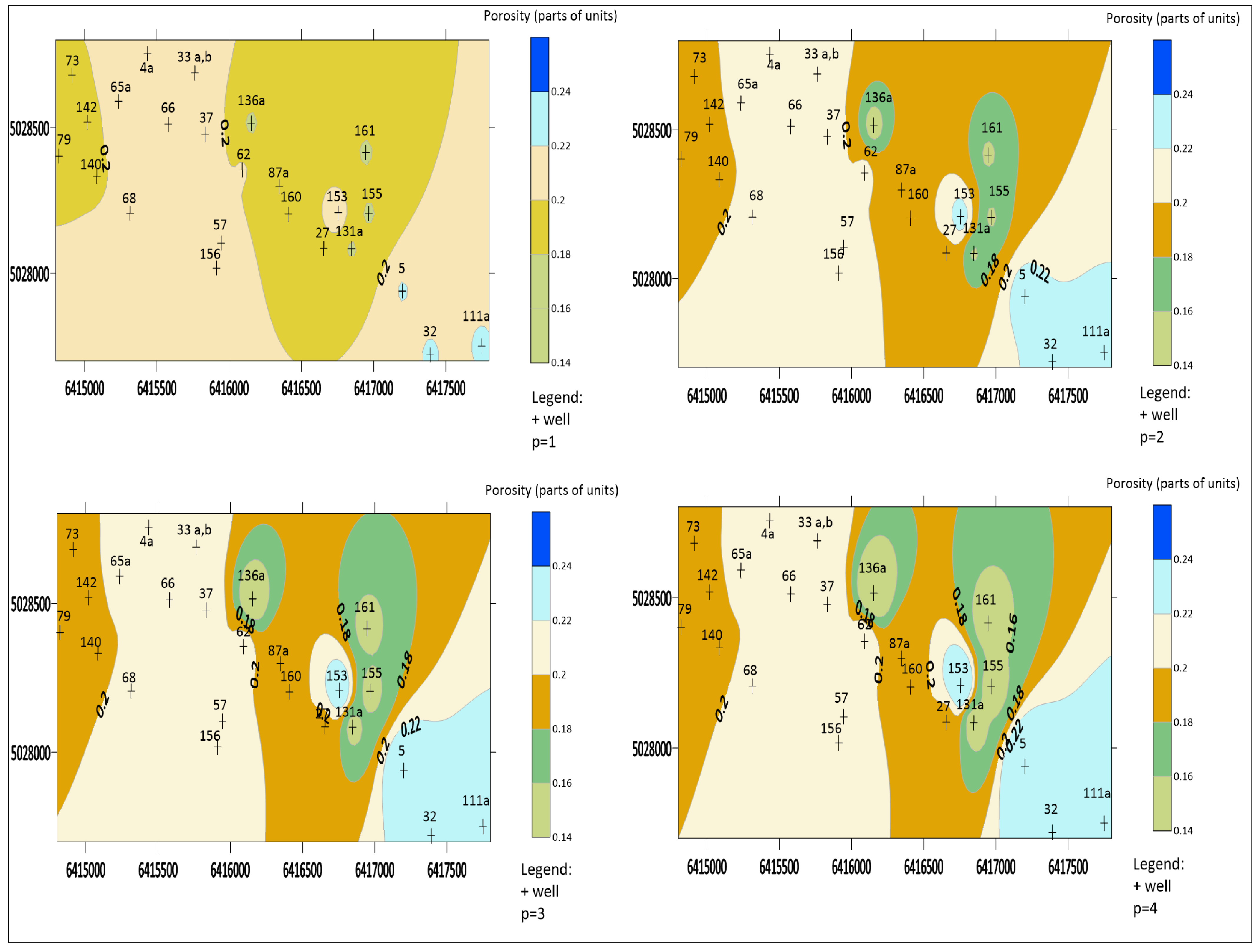
A qualitative analysis of interpolated maps implies a visual inspection of the map and the existence of the following visual mapping results: bull’s-eye (circular), butterfly (ellipsoidal) and mosaic [32]. During the visual analysis of the maps, maps with a value of p = 0 were not analyzed, because according to Equation (1), in that case the solution of the equation would be the same. The results of the mapping of reservoirs K and L using the IDW method for p values of 1, 2, 3 and 4 are shown in Figure 2 and Figure 3.
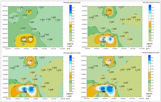
Figure 2.
Maps of the porosity of the K reservoir obtained by the IDW method for values of p = 1, 2, 3, 4.
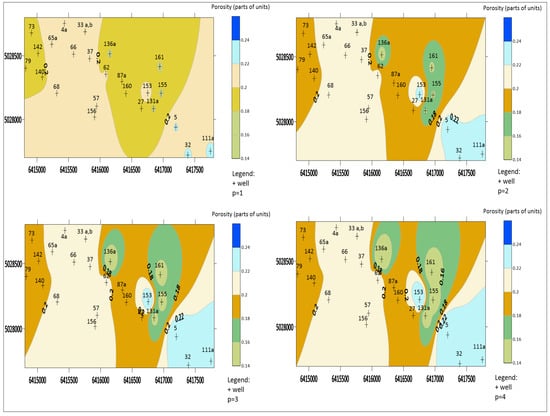
Figure 3.
Maps of the porosity of the L reservoir obtained by the IDW method for values of p = 1,2,3,4.
In the case of reservoir K (see Figure 2), with an increasing value of p, a pronounced bulls-eye effect (p = 1, p = 2) and butterfly effect (p = 3, p = 4) appears. At higher values, as seen with J-25, J-168, etc., regardless of the change in the value of p, the effect was not removed, but the changes were detected as a pronounced bulls-eye effect changing into a butterfly effect. With an increase in the value of p, there was no mosaic effect, which is positive. The transition zones were different in all cases of a change in p; the clearest transition zone was seen in the case of p = 2, and it did not have such a pronounced asymmetric value change as in the other cases. Also, a p value of 2 can reduce the number of bull’s-eyes to show only extreme values in the input data. In cases where bull’s-eye and butterfly effects are expressed on the maps, from a visual point of view, interpolated maps with a bulls-eye effect are preferred. With the bull’s-eye effect, the value is evenly distributed around the point data, while with the butterfly effect, there is an ellipsoidal surface around the point data, which due to its appearance can encompass more space, which is not realistic. Therefore, for the example of the interpolated map obtained in Figure 2, i.e., in the case of a small data set, the value of p is 1 and 2 when using the IDW method.
The porosity map of reservoir L (see Figure 3) has a pronounced butterfly effect for all cases of p values. As the value of p increases in this case, the bull’s-eye and mosaic effect are not present, which is evident from the obtained interpolation map. The reason for this is that it is a large data set, and the input data set is sufficient to perform a satisfactory interpolation in the given area. The transition area between different input data values is clearer when interpolating with p values of 3 and 4. For p values of 3 and 4, it is very clear that reservoir L is tectonically very clearly divided and the stability of transition zones is conditioned by the relative values of individual data with neighboring ones, which can be seen in the eastern parts of the interpolated maps as a rather asymmetric area of porosity values. Considering the transition zones and the inclusion of input data in the interpolated maps, for a large data set, the recommendation from the visual inspection of the maps is to use p values of 3 and 4 when applying the IDW method.
4.2. Quantitative Analysis of Maps
The quantitative analysis was expressed by the numerical values of RMSE, MAE and MAD, the results of which are shown in Table 3 for the K and L reservoirs.

Table 3.
RMSE, MAE and MAD values for different values of p for the K and L reservoirs.
The values of RMSE and MAE for reservoir K increased as the value of the coefficient p increased, while the value of MAD varied. The RMSE values were 0.00104–0.00155, and the values of MAE were 0.01700–0.02319, which shows continuous but almost linear growth. The MAD values were not linear and had values of 0.00360–0.00734. According to the RMSE, MAE and MAD values, the smallest values on the interpolated porosity map of reservoir K were with p values of 1 and 2. Unlike reservoir K, the RMSE, MAE and MAD values for reservoir L were not in a linear relationship. RMSE values were 0.0263–0.02470, MAE values were 0.01924–0.01490 and MAD values were 0.00869–0.00343. As can be seen from Table 3, it was for a value of p of 1 that reservoir L had the highest values on the interpolated porosity map, while for values of p of 3 and 4, it had the lowest values. According to the quantitative methods and the RMSE, MAE and MAD values, for a small sample, the optimal value of p is 1 or 2, while for a large sample, the optimal value of p is 3 or 4.
4.3. Qualitative–Quantitative Approach in Selection of p-Value
Most of the authors who have analyzed p values for the IDW method have used a large data set. Moreover, IDW is one of the most applied interpolation methods overall in many sciences that deal with spatial data, e.g., in mining [33] or soil mapping for military applications [34]. However, the selection of a p-value to be the standard for any scientific field is a very hard, if not impossible, task, and it often depends not only on the discipline, but also on the geographical location of data. Such a geographically specific analysis is presented here as an example of subsurface geological mapping in the northern Croatia Neogene sandstones, and the geological background defined what were considered as “small” and “large” data sets (in some other disciplines and locations, such definitions could be totally different).
4.4. Discussion
All the applied data and methods in this research included some uncertainties. For this reason, both data sets were considered for the comprehensive p-value analysis, including both qualitative and quantitative analyses, that was used for the hydrocarbon reservoirs K and L of Lower Pontian age.
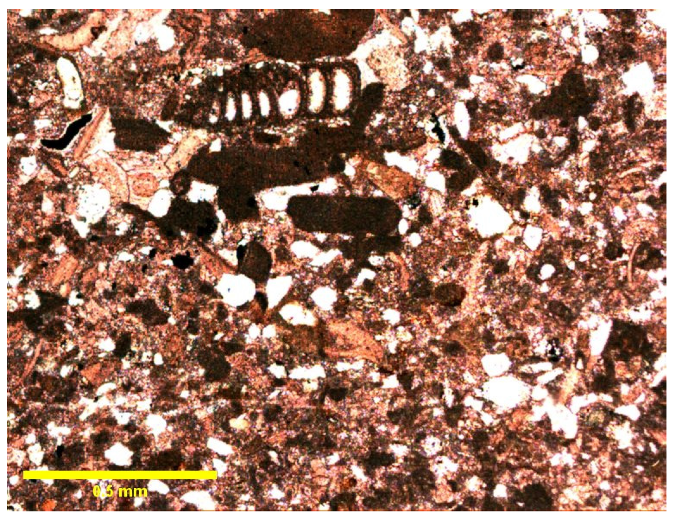
Looking only at the numerical values of the RMSE, MAE and MAD could lead to the conclusion that only the lowest values are criteria for the “best” p-value. Obviously, this could be a wrong and misleading approach. It is valid especially because the Neogene northern Croatian sandstones are often of very heterogeneous porosity, including primary and secondary ones, as a result of compaction and dissolutions, as shown in Figure 4 for Middle Miocene sandstones.

Figure 4.
A photomicrograph of the typical Middle Miocene calcarenite from northern Croatia. Mixed various silt-to-sand size, poorly sorted, angular carbonate bioclasts and siliciclastic grains (predominantly quartz) embedded in carbonate matrix. Primary intergranular and intragranular porosity partly reduced by calcite cementation.
The Upper Miocene calcarenite (see Figure 4) developed from the Middle Miocene ones, giving the same complexity of inter- and intragranular space as well as detritus composition. For example, the L reservoir sandstones are typical Lower Pontian deposits in the Sava Depression, with a high proportion of silt (silty sandstones) decreasing their “homogeneity” and “isotropy”, i.e., reservoir quality. Calcite detritus in matrix is abundant, which makes it the dominant material for dissolution and subsequent calcite cementation. This is similarly valid for the K reservoir sandstone. Consequently, although the log porosity often surpasses 20%, their values are hardly precisely determined from logs (often the values are very similar in different wells). Moreover, silty components influenced reservoir porosity variations in intervals of a few percent, but also made it very unpredictable because the differences in detritus sources are hard to interpret in such small structures. Eventually, the result is a reservoir lithologically fragmented in zones of lower petrophysical values, which makes production challenging over years, requiring the permanent fitting of a producing regime and injection well network.
Due to the inherited and numerically indescribable uncertainties belonging to a reservoir space, it is obligatory to also use a quantitative approach. This implies visually inspecting the porosity maps and eliminating ones where some impossible subsurface shapes exist (like butterfly or too strong bull’s-eye effects), or known faults with distorted isoporosity lines of continuity. Using both criteria, quantitative and qualitative, it is clear that for a small data set (like the K reservoir), the optimal p is 2, while for a large data set (like the L reservoir), the optimal value is 3 or 4. This is a recommendation for the application of the IDW method in the porosity mapping of northern Croatia’s Lower Pontian sandstones, at least in the subsurface of the Sava Depression, while it is also definitely recommended for other sciences for analyzing input data sets and performing a quantitative–qualitative analysis.
5. Conclusions
Data sets in geosciences are dispersed and in most cases are presented in the form of limited data sets (often less than a hundred data, sometimes even less than a dozen). Two of these were analyzed for the porosity data of the K and L hydrocarbon reservoirs of the Lower Pontian age in northern Croatia. The main results of the analysis were:
- -
- Qualitative 1: For a small data set (19 data, the K reservoir), it is recommended to use a p-value of 2, because in this case, the butterfly effect is eliminated, and the RMSE value of 0.00119, MAE value of 0.02103, and MAD value of 0.00546 are smaller compared to those found using larger p values.
- -
- Qualitative 2: The p values of 3 and 4 are optimal in the case of a large data set (25 data, the L reservoir) because the transition zones are clear and the input data set is included, and this is confirmed by the following values: RMSE (0.02435, 0.02437), MAE (0.01582, 0.01509) and MAD (0.00896, 0.00444).
- -
- Quantitative 1: Data dispersion is present in the cases of a small and a large data set, and when changing the value of p, it gradually affects the isoporosity shapes on obtained interpolation maps.
- -
- Quantitative 2: The IDW method in both cases gave usable results, and due to the similar lithologies in most of the Sava Depression (northern Croatia), it is recommended to apply the IDW method with p-values between 2 and 4, depending on the size of the analyzed porosity data set.
- -
- Quantitative 3: The IDW is especially recommended for use when a spatial model calculated by, e.g., variogram includes large uncertainties expressed in a high nugget effect and a low number of data pairs for each lag.
Author Contributions
Conceptualization, J.I., U.B and T.M.; methodology J.I., U.B and T.M.; validation, J.I., U.B and T.M; investigation, J.I.; writing—original draft preparation, J.I. and U.B.; writing—review and editing, J.I., U.B and T.M.; visualization, J.I. All authors have read and agreed to the published version of the manuscript.
Funding
This research received no external funding.
Data Availability Statement
The data is contained within the article.
Acknowledgments
The authors thank the anonymous reviewers and editors for their generous and constructive comments that have improved this paper. This research was partially carried out within the project “Mathematical researching in geology VIII & IX” (led by T. Malvić).
Conflicts of Interest
The authors declare no conflicts of interest.
References
- Bartier, P.M.; Keller, C.P. Multivariate interpolation to incorporate thematic surface data using inverse distance weighting (IDW). Comput. Geosci. 1996, 22, 795–799. [Google Scholar] [CrossRef]
- Gossel, W.; Falkenhagen, M. Line-Geometry-Based Inverse Distance Weighted Interpolation (L-IDW): Geoscientific Case Studies. In Proceedings of the Mathematics of Planet Earth: Proceedings of the 15th Annual Conference of the International Association for Mathematical Geosciences, Berlin, Germany, 8 October 2013; Springer: Berlin, Germany. [Google Scholar] [CrossRef]
- Karami, R.; Afzal, P. Estimation of Elemental Distributions by Combining Artificial Neural Network and Inverse Distance Weighted (IDW) Based on Lithogeochemical Data in Kahang Porphry Deposit, Central Iran. Univers. J. Geosci. 2015, 3, 59–65. [Google Scholar] [CrossRef]
- Srinivas, V.S.; Sarma, A.D.; Achanta, H.K. Modeling of Ionospheric Time Delay Using Anisotropic IDW with Jackknife Technique. IEEE Trans. Geosci. Remote Sens. 2016, 54, 513–519. [Google Scholar] [CrossRef]
- Mircovski, V.; Gicevski, B.; Dimov, G. Hydrochemical characteristics of the groundwaters in Prilep’s part of Pelagonia valley—Republic of Macedonia. Rud.-Geološko-Naft. Zb. 2018, 33, 111–119. [Google Scholar] [CrossRef]
- Maliqi, E.; Idrizi, B.; Penev, P. Compilation of groundwater monitoring maps for the Mitrovica region in Kosova. Geosci. Remote Sens. 2019, 2, 41–55. [Google Scholar] [CrossRef]
- Sun, L.; Wei, Y.; Cai, H.; Yan, J.; Xiao, J. Improved Fast Adaptive IDW Interpolation Algorithm based on the Borehole Data Sample Characteristic and Its Application. In Proceedings of the 3rd International Conference on Data Mining, Communications and Information Technology, Beijing, China, 24–26 May 2019. [Google Scholar] [CrossRef]
- Pulatov, A.; Khamidov, A.; Akhmatov, D.; Pulatov, B.; Vasenev, V. Soil salinity mapping by different interpolation methods in Mirzaabad district, Syrdarya Province. In Proceedings of the International Scientific Conference Construction Mechanics, Hydraulics and Water Resources Engineering, Tashkent, Uzbekistan, 23–25 April 2020. [Google Scholar] [CrossRef]
- Gonzales, R.; Rahardi, M.R.G.; Octova, A. Estimation of tin resources using Inverse distance weighted (IDW) and nearest neighbor point (NNP) methods in Bangka Tengah district, Bangka Belitung islands province. Georest 2023, 2, 1–7. [Google Scholar] [CrossRef]
- Đurđević, B.; Jug, I.; Jug, D.; Bogunović, I.; Vukadinović, V.; Stipešević, B.; Brozović, B. Spatial variability of soil organic matter content in Eastern Croatia assessed using different interpolation methods. Int. Agrophys. 2019, 33, 31–39. [Google Scholar] [CrossRef] [PubMed]
- Mesić Kiš, I. Comparison of ordinary and universal Kriging interpolation techniques on a depth variable (a case of linear spatial trend), case study of the Šandrovac field. Rud.-Geološko-Naft. Zb. 2016, 31, 41–58. [Google Scholar] [CrossRef]
- Novak Zelenika, K.; Novak Mavar, K.; Brnada, S. Comparison of the Sweetness Seismic Attribute and Porosity–Thickness Maps, Sava Depression, Croatia. Geosciences 2018, 8, 426. [Google Scholar] [CrossRef]
- Novak Zelenika, K.; Malvić, T. Stochastic simulations of dependent geological variables in sandstone reservoirs of Neogene age: A case study of Kloštar Field, Sava Depression. Geol. Croat. 2011, 64, 173–183. [Google Scholar] [CrossRef]
- Achilleos, G.A. The Inverse Distance Weighted interpolation method and error propagation mechanism—creating a DEM from an analogue topographical map. J. Spat. Sci. 2011, 56, 283–304. [Google Scholar] [CrossRef]
- Maleika, W. Inverse distance weighting method optimization in the process of digital terrain model creation based on data collected from a multibeam echosounder. Appl. Geomat. 2020, 12, 397–407. [Google Scholar] [CrossRef]
- Liu, Z.; Zhang, Z.; Zhou, C.; Ming, W.; Du, Z. An Adaptive Inverse-Distance Weighting Interpolation Method Considering Spatial Differentiation in 3D Geological Modeling. Geosciences 2021, 11, 51. [Google Scholar] [CrossRef]
- Yadav, S.K.; Singh, S.; Gupta, R. Measures of Dispersion. In Biomedical Statistics; Springer: Singapore, 2019; pp. 59–71. [Google Scholar] [CrossRef]
- Botta-Dukát, Z. Quartile coefficient of variation is more robust than CV for traits calculated as a ratio. Sci. Rep. 2023, 13, 4671. [Google Scholar] [CrossRef] [PubMed]
- Browne, M.W. Cross-Validation Methods. J. Math. Psychol. 2000, 44, 108–132. [Google Scholar] [CrossRef] [PubMed]
- Rodríguez, J.D.; Martínez, A.P.; Lozano, J.A. Sensitivity Analysis of k-Fold Cross Validation in Prediction Error Estimation. IEEE Trans. Pattern Anal. Mach. Intell. 2010, 32, 569–575. [Google Scholar] [CrossRef] [PubMed]
- Chai, T.; Draxler, R.R. Root mean square error (RMSE) or mean absolute error (MAE)?—Arguments against avoiding RMSE in the literature. Geosci. Model Dev. 2014, 7, 1247–1250. [Google Scholar] [CrossRef]
- Ćalasan, M.; Abdel Aleem, S.H.E.; Zobaa, A.F. On the root mean square error (RMSE) calculation for parameter estimation of photovoltaic models: A novel exact analytical solution based on Lambert W function. Energy Convers. Manag. 2020, 210, 112716. [Google Scholar] [CrossRef]
- Willmott, C.J.; Kenji, M. Advantages of the mean absolute error (MAE) over the root mean square error (RMSE) in assessing average model performance. Clim. Res. 2005, 30, 79–82. [Google Scholar] [CrossRef]
- Hodson, T.O. Root-mean-square error (RMSE) or mean absolute error (MAE): When to use them or not. Geosci. Model Dev. 2022, 15, 5481–5487. [Google Scholar] [CrossRef]
- Pham-Gia, T.; Hung, T.L. The mean and median absolute deviations. Math. Comput. Model. 2001, 34, 921–936. [Google Scholar] [CrossRef]
- Elamir, E. Mean Absolute Deviation about Median as a Tool of Explanatory Data Analysis. Int. J. Recent Res. Appl. Stud. 2012, 11, 517–523. [Google Scholar]
- Ivšinović, J.; Malvić, T. Application of the radial basis function interpolation method in selected reservoirs of the Croatian part of the Pannonian Basin System. Min. Miner. Depos. 2020, 14, 37–42. [Google Scholar] [CrossRef]
- Ivšinović, J.; Pimenta Dinis, M.A.; Malvić, T.; Pleše, D. Application of the bootstrap method in low-sampled Upper Miocene sandstone hydrocarbon reservoirs: A case study. Energy Sources Part A Recovery Util. Environ. Eff. 2021, 41, 1–15. [Google Scholar] [CrossRef]
- Ivšinović, J. Selection and Geomathematical Calculation of Variables for Sets with Less than 50 Data Regarding the Creation of an Improved Subsurface Model, Case Study from the Western Part of the Sava Depression. Ph.D. Thesis, University of Zagreb, Faculty of Mining, Geology and Petroleum Engineering, Zagreb, Croatia, 2019. Available online: https://urn.nsk.hr/urn:nbn:hr:169:977620 (accessed on 27 May 2024).
- Malvić, T.; Ivšinović, J.; Velić, J.; Rajić, R. Kriging with a Small Number of Data Points Supported by Jack-Knifing, a Case Study in the Sava Depression (Northern Croatia). Geosciences 2019, 9, 36. [Google Scholar] [CrossRef]
- Malvić, T.; Ivšinović, J.; Velić, J.; Rajić, R. Interpolation of Small Datasets in the Sandstone Hydrocarbon Reservoirs, Case Study of the Sava Depression, Croatia. Geosciences 2019, 9, 201. [Google Scholar] [CrossRef]
- Ivšinović, J.; Malvić, T. Comparison of mapping efficiency for small datasets using inverse distance weighting vs. moving average, Northern Croatia Miocene hydrocarbon reservoir. Geologija 2022, 65, 47–57. [Google Scholar] [CrossRef]
- Rezaei, M.; Fallahi, S. Block model optimization and resource estimation of the Angouran Mine by transferring the exploratory data from the local coordinate system to the UTM. Rud.-Geološko-Naft. Zb. 2023, 38, 1–17. [Google Scholar] [CrossRef]
- Heštera, H.; Pahernik, M.; Kovačević Zelić, B.; Maurić Maljković, M. The Unified Soil Classification System Mapping of the Pannonian Basin in Croatia using Multinominal Logistic Regression and Inverse Distance Weighting Interpolation. Rud.-Geološko-Naft. Zb. 2023, 38, 147–159. [Google Scholar] [CrossRef]
Disclaimer/Publisher’s Note: The statements, opinions and data contained in all publications are solely those of the individual author(s) and contributor(s) and not of MDPI and/or the editor(s). MDPI and/or the editor(s) disclaim responsibility for any injury to people or property resulting from any ideas, methods, instructions or products referred to in the content. |
© 2024 by the authors. Licensee MDPI, Basel, Switzerland. This article is an open access article distributed under the terms and conditions of the Creative Commons Attribution (CC BY) license (https://creativecommons.org/licenses/by/4.0/).

