Google Earth Engine and Machine Learning for Flash Flood Exposure Mapping—Case Study: Tetouan, Morocco

Abstract

Recently, the earth’s climate has changed considerably, leading to several hazards, including flash floods (FFs). This study aims to introduce an innovative approach to mapping and identifying FF exposure in the city of Tetouan, Morocco. To address this problem, the study uses different machine learning methods applied to remote sensing imagery within the Google Earth Engine (GEE) platform. To achieve this, the first phase of this study was to map land use and land cover (LULC) using Random Forest (RF), a Support Vector Machine (SVM), and Classification and Regression Trees (CART). By comparing the results of five composite methods (mode, maximum, minimum, mean, and median) based on Sentinel images, LULC was generated for each method. In the second phase, the precise LULC was used as a related factor to others (Stream Power Index (SPI), Topographic Position Index (TPI), Slope, Profile Curvature, Plan Curvature, Aspect, Elevation, and Topographic Wetness Index (TWI)). In addition to 2024 non-flood and flood points to predict and detect FF susceptibility, 70% of the dataset was used to train the model by comparing different algorithms (RF, SVM, Logistic Regression (LR), Multilayer Perceptron (MLP), and Naive Bayes (NB)); the rest of the dataset (30%) was used for evaluation. Model performance was evaluated by five-fold cross-validation to assess the model’s ability on new data using metrics such as precision, score, kappa index, recall, and the receiver operating characteristic (ROC) curve. In the third phase, the high FF susceptibility areas were analyzed for two-way validation with inundated areas generated from Sentinel-1 SAR imagery with coherent change detection (CDD). Finally, the validated inundation map was intersected with the LULC areas and population density for FF exposure and assessment. The initial results of this study in terms of LULC mapping showed that the most appropriate method in this research region is the use of an SVM trained on a mean composite. Similarly, the results of the FF susceptibility assessment showed that the RF algorithm performed best with an accuracy of 96%. In the final analysis, the FF exposure map showed that 2465 hectares were affected and 198,913 inhabitants were at risk. In conclusion, the proposed approach not only allows us to assess the impact of FF in this study area but also provides a versatile approach that can be applied in different regions around the world and can help decision-makers plan FF mitigation strategies.

1. Introduction

According to researchers’ findings, there is a clear link between global warming and industrialization, as shown by the many ecological imbalances that have arisen in recent years and have led to several disasters, the most significant of which is flooding. Depending on their location, floods are divided into three categories: River Floods, Coastal Floods, and Flash Floods (FF). Due to their rapid occurrence, high speed, and destructive effect, FFs are among the world’s deadliest natural disasters [1]. This also applies to Morocco, which has suffered from several FFs, the most significant of which are the Mohammadia flood [2], the Oued Ourika FF [3], the Guelmim region flood [4,5], and the Tetouan FF [6].

One reason FFs are so hazardous is that they commonly happen in metropolitan areas, where there is a high concentration of impervious surfaces that contribute significantly to urban FFs [7].

Impervious surfaces, slope, soil type, land use, rainfall intensity, and duration are among the major factors in FFs. Understanding the variables that affect the probability of FF occurrence in a given area is very important, and this can be done in several ways, including determining FF susceptibility. Prior studies have demonstrated the value of FF susceptibility mapping in disaster management. As time passed, different methods were developed in this sense, such as Dempster–Shafer [8], frequency ratio [9], weights of evidence (WofE) [10], index of entropy [11], the analytical hierarchy process [12], fuzzy logic [13], and the Machine learning and deep learning approach (ML and DL) [14]. Because of their ability to process significant volumes of complicated data and recognize and predict future patterns, Machine Learning (ML) and Deep Learning (DL) techniques have recently demonstrated their effectiveness in accurately identifying and predicting FF susceptibility. Consequently, these approaches are considered the best for such modeling. Contrary to traditional methods that directly determine weights, ML and DL learn weights through the training process, enabling complex relationships to be found between FF risk and its influencing factors. This was the case in the study of Shreevastav et al. [15], which adopted the same approach to assess flood risk modeling in the lower Bagmati river region of Eastern Terai, Nepal, using the ML model of MaxEnt. Moreover, Al-Areeq et al.’s [16] research used a logistic model tree (LT), a Bagging ensemble (BE), k-nearest neighbors, and a kernel support vector machine to map Jeddah, Saudi Arabia’s flood vulnerability. In Karachi, Pakistan, by combining a novel set model of Multi-Layer Perceptron, Support Vector Machine, and Logistic Regression (LR), which additionally assesses influencing variables, Yaseen et al. [17] created a flood susceptibility map.

It should be emphasized that mapping FF susceptibility using the ML approach requires two types of variables to feed the model, the dependent variable (1) and the independent variable (2):

(1): The dependent variable represents the FF and non-FF areas and can be collected using a variety of techniques, with field survey and satellite remote sensing techniques being the most useful. However, due to the conditions and flash occurrence of this phenomenon, it is not always possible to process a field survey. For this reason, many studies focus on remote sensing techniques to estimate the extent of FFs using satellite imagery, especially synthetic aperture radar SAR data [18,19,20], with sensors able to pierce clouds and heavy rainfall during FFs and post-flood events [19].

(2): The independent variable, on the other hand, indicates the climatic, hydrological, and geographical conditions that affect the event’s occurrence. Among these factors are the topographic wetness index (TWI), stream power index (SPI), flow accumulation (FA), plan curvature (PC), convergence index (CI), topographic position index (TPI), elevation, aspect, slope, and LULC. The last factor is the variable with the highest impact; hence, the correct mapping of LULC is extremely important.

Most studies in recent years have attempted to map LULC using cloud computing platforms such as GEE, which is considered an all-in-one cloud computing platform with an archive of petabytes of geospatial data freely available for visualization and analysis without having to download data or work on local software. It also enables quick selection of the best satellite imagery based on multiple criteria, the use of specific aggregation functions, and the comparison of different compositions to process the best classification. As an example, the research by Liu et al. [21] employed time series data from GEE and a random forest model in Ganan Prefecture to generate LULC change. Similarly, Feizizadeh et al. [22] employed ML techniques on GEE in Northern Iran to assess changes in LULC based on a time series image of Landsat. In addition, Nasiri et al.’s study [23] compared two composition techniques using GEE for producing precise LULC maps over Tehran Province (Iran) using Sentinel-2 and Landsat-8. LULC is not only among the factors that contribute to FF susceptibility but is also considered a key element of FF exposure.

The FF is a localized flood that happens quickly and lasts for a short time (less than 6 h). It is caused by intense precipitation in a small watershed (often less than 100 km²) [24,25]. This makes it difficult for authorities to respond effectively to the recovery processes. Determining exposure—the position, physical qualities, and cost of resources that are essential to communities (people, buildings, businesses, agriculture, etc.)—in a fast way is necessary. In response to the previous difficulty, several researchers have turned to the prospect of using GEE because it offers a viable solution concerning rapid analysis and data availability for rapid exposure determination, such as in the study of Shinde et al. [18], which proposed a semi-automatic flood mapping system as a quick analysis method for impact analysis and damage assessment utilizing GEE. Pandey et al. [20] employed the Synthetic Aperture Radar (SAR) Sentinel-1A at GEE to monitor widespread floods in the Ganga-Brahmaputra region in 2020 and to calculate the effects of flooding on agriculture and people. To our knowledge, most studies that have used GEE for flood and FF damage assessment use existing LULC datasets (e.g., Copernicus Global Land Cover Layers) rather than creating an accurate LULC map based on high-resolution satellite imagery of the region in question even though it can provide a higher level of identification and specificity, given that the accurate assessment of events requires accurate LULC mapping.

In addition, recent evidence has shown that using GEE to monitor flooding is practical, informative, and user-friendly for decision-makers [26,27,28,29,30]. The availability of quickly accessible data is a factor that all researchers agree on. In the context of flooding, SAR data are most commonly used to determine their extent [20]. However, it is not always available due to the temporal resolution of the satellites, especially in the case of FFs, which are characterized by their rapid occurrence. Therefore, the satellite may occasionally not reach the location of the event; it may take several days or even weeks before it returns to that location and collects new data. Therefore, in situations where SAR data are not available, ML models can be used as a valuable surrogate to determine the hazard of FFs based on other available data sources such as historical FF records as well as climatic, hydrological, and geographical data. However, even when SAR data are available, the use of ML to quantify FF susceptibility can help improve and validate the results obtained from SAR analysis. This is because SAR data only provide information on the extent and severity of flooding or FFs, whereas FF susceptibility models can provide additional information on fundamental variables that influence the occurrence of the event at a particular location. In addition, it is important to assess the damage caused by FFs, identify the most affected regions, and prioritize the allocation of resources for reconstruction and rehabilitation. The results of FF susceptibility or SAR data can help with these assessments by properly supporting details about the type of event and the locations affected.

Motivated by recent challenges, a new initiative is proposed that breaks new ground in FF mapping by providing a comprehensive and rigorous framework that utilizes diverse datasets, explores a range of ML algorithms, and evaluates performance across multiple metrics. This study focuses on the major FF that occurred on 1 March 2021, in the northern Moroccan city of Tetouan and presents a precise strategy for detecting and mapping FF damage. Using a comparison of many composite methods (max, min, mean, and median) trained on different machine learning models (SVM, CART, and RF), the LULC will first be mapped. The accurately determined LULC will be one of the criteria for predicting FF susceptibility using several ML methods (SVM, RF, LR, NB, and MLP). The FF extent will also be extracted using SAR data, and the exposure assessment will be concluded by overlaying all obtained data.

2. Materials and Methods

2.1. Study Area

The city of Tetouan is located in the region of Tangier–Tetouan–Al Hoceima, in the far north of the western Rif mountain range in the northwest of the Moroccan kingdom (Figure 1), precisely in the center of the Martil Valley, between the mountains of Darsa to the north and Gorghiz to the south, about sixty kilometers east of Tangier, forty-one kilometers south of the Strait of Gibraltar, and ten kilometers from the Mediterranean Sea. It has an area of 2541 km² and a population of 578,283 inhabitants compared to 157,684 inhabitants in the countryside.

The climate of Tetouan is a Mediterranean one, with wet and rainy winters, dry and moderately hot summers, and temperatures that range from a low of 8.5 °C to a high of 29.3 °C. The annual precipitation amount varies considerably ranging between 326 mm as the minimum recorded and 1291 mm as the maximum; however, according to the measurements recorded over the last 30 years, the annual precipitation rate stabilizes at 728 mm. Geologically, Tetouan, which is part of the Rif Mountains’ internal range, is distinguished by numerous different kinds of structural units: (1) the Ghomarides, which are metamorphic nappes of the Paleozoic from the Silurian to the Carboniferous. (2) The Sebtides, which are composed of polymetamorphic terrains and Paleozoic–Triassic cover. (3) The Calcareous Dorsal. (4) Flysch. The old city of Tetouan climbs on a slope from the river and appears to tower over anyone approaching from the south and west. Tetouan is subject to a range of geo-environmental risks because of its unique topographical and geological characteristics. The area’s greatest threat is the FFs that occurred on 24 December 2009, 29 August 2013, 20 February 2016, 5 March 2018, 1 March 2021, 5 April 2022, 2 June 2023, and 31 March 2024.

2.2. Data

In this study, four different types of data were used: (1) Satellite imagery (Figure 2A); (2) Digital elevation model (DEM) (Figure 2B); (3) Population density (Figure 2C); (4) FF and non-FF points (Figure 2D).

2.2.1. Satellite Imagery

Satellite imagery is an indispensable resource for understanding and solving the world’s complex problems and disasters, such as FFs [31]. With its robust and distinctive perspective on the Earth’s surface, it allows us to study and monitor the environment, natural resources, and human activities on a global and local scale. In this study, the harmonized Sentinel-2 MSI: Multispectral Instrument Level-2A and SENTINEL-1 SAR-Ground Range Detected (GRD) Level-1 were used for mapping the extent of LULC and FFs, respectively.

Four bands with a spatial resolution of 10 m, six bands with a resolution of 20 m, and three bands with a resolution of 60 m together form the harmonized multispectral instrument (MSI)—SENTINEL-2 (

Table 1. Key information about the Sentinel-2MSI/S2A: Sentinel-2A and S2B: Sentinel-2B.

Name	Pixel Size	Wavelength
B1: Aerosols	60 m	S2A: 443.9 nm	(S2B): 442.3 nm
B2: Blue	10 m	S2A: 496.6 nm	(S2B): 492.1 nm
B3: Green	10 m	S2A: 560 nm	(S2B): 559 nm
B4: Red	10 m	S2A: 664.5 nm	(S2B): 665 nm
B5: Red Edge 1	20 m	S2A: 703.9 nm	(S2B): 703.8 nm
B6: Red Edge 2	20 m	S2A: 740.2 nm	(S2B): 739.1 nm
B7: Red Edge 2	20 m	S2A: 782.5 nm	(S2B): 779.7 nm
B8: NIR	10 m	S2A: 835.1 nm	(S2B): 833 nm
B8A: Red Edge 3	20 m	S2A: 864.8 nm	(S2B): 864 nm
B9: Water vapor	60 m	S2A: 945 nm	(S2B): 943.2 nm
B10: Cirrus	60 m	S2A: 1373.5 nm	(S2B): 1376.9 nm
B11: SWIR 1	20 m	S2A: 1613.7 nm	(S2B): 1610.4 nm
B12: SWIR 2	20 m	S2A: 2202.4 nm	(S2B): 2185.7 nm

), with a temporal resolution of 10 days with one satellite at the equator and 5 days with two satellites in clear sky conditions. (https://developers.google.com/earth-engine/datasets/catalog/COPERNICUS_S2_SR_HARMONIZED; accessed on 21 March 2024).

The Ground Range Detected (GRD)—Level-1, which was developed as part of the SENTINEL-1 SAR mission, is a radar imager providing permanent, day and night, all-weather coverage in the dual C-band polarization channels (VH and VV). The spatial resolution is 10 m and the temporal resolution is 12 days. (https://sentinel.esa.int/web/sentinel/missions/sentinel-1; accessed on 21 March 2024).

2.2.2. Digital Elevation Model

DEM is the abbreviation for Digital Elevation Model, which is a digital representation of the terrain’s topography. Topographic surveys, stereoscopic aerial photographs, satellite images, and other data sources are used to create a DEM. The topographic map in its raw digital format was the source for the DEM data used in this study (Tetouan AL AZHAR—NI-30-XIX-4-a-1 at 1/25,000 scale of 2018 and Tetouan Sidi Al Mandri—NI-30-XIX-4-a-2 at 1/25,000 scale of 2018) and was provided by the National Agency of Land Registry, Cadastre and Cartography of Morocco—ANCFCC. The topographic map was created from aerial photographs taken in March 2015 using analytical photogrammetry techniques and validated during a field survey in May 2018. The generated DEM has a resolution of 10 m and was created based on the elevation part of our digital map with a vertical equidistance of 5 m between the contour lines. To avoid uncertainties in the dataset, we implemented further analysis to determine the sink depth and then applied a fill and sink removal procedure using ArcGIS Pro 3.2.

2.2.3. Flash Flood and Non-Flash-Flood Areas

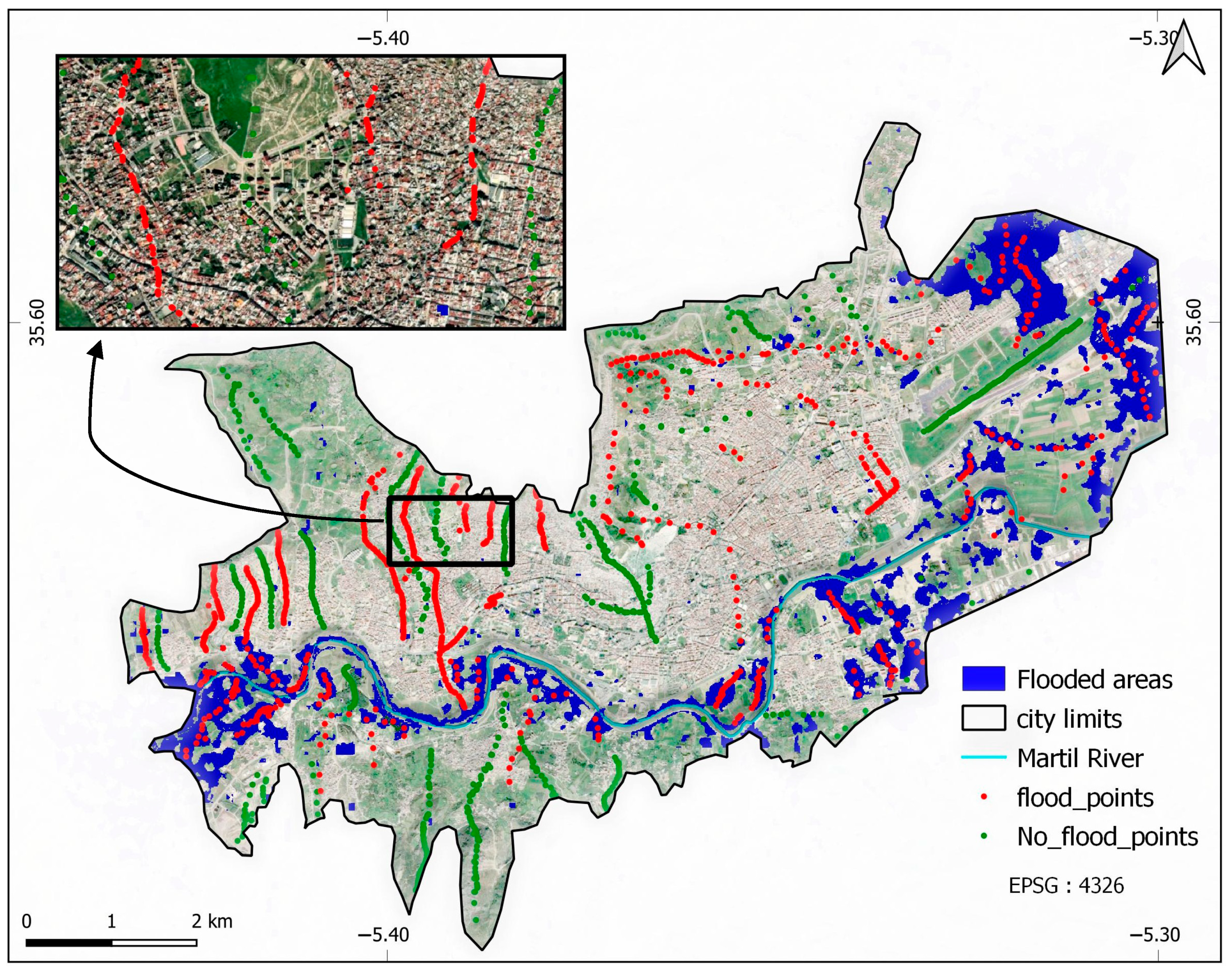
In determining susceptibility to FF, the locations of FF-prone and non-FF-prone areas are critical for feeding machine learning algorithms. The urban FF on 1 March 2021 was used to collect information on FF and non-FF areas. During this period, we conducted a field study at our research sites. We used a portable GNSS receiver to determine the ideal location of flooded and non-flooded points. A total of 2024 points were located, of which 1175 were flooded and the rest were not flooded.

2.2.4. Population Density

A population density map graphically shows the distribution of people in a given area. Using a population density map to identify geographic patterns of population distribution can help determine the urgency of the emergency and support pre- and post-incident assessment tactics. The population density map (available in the 2016–2021 monograph of the municipality of Tetouan) used in this study was combined with LULC to identify the exposed population and assess the damage.

2.3. Methods

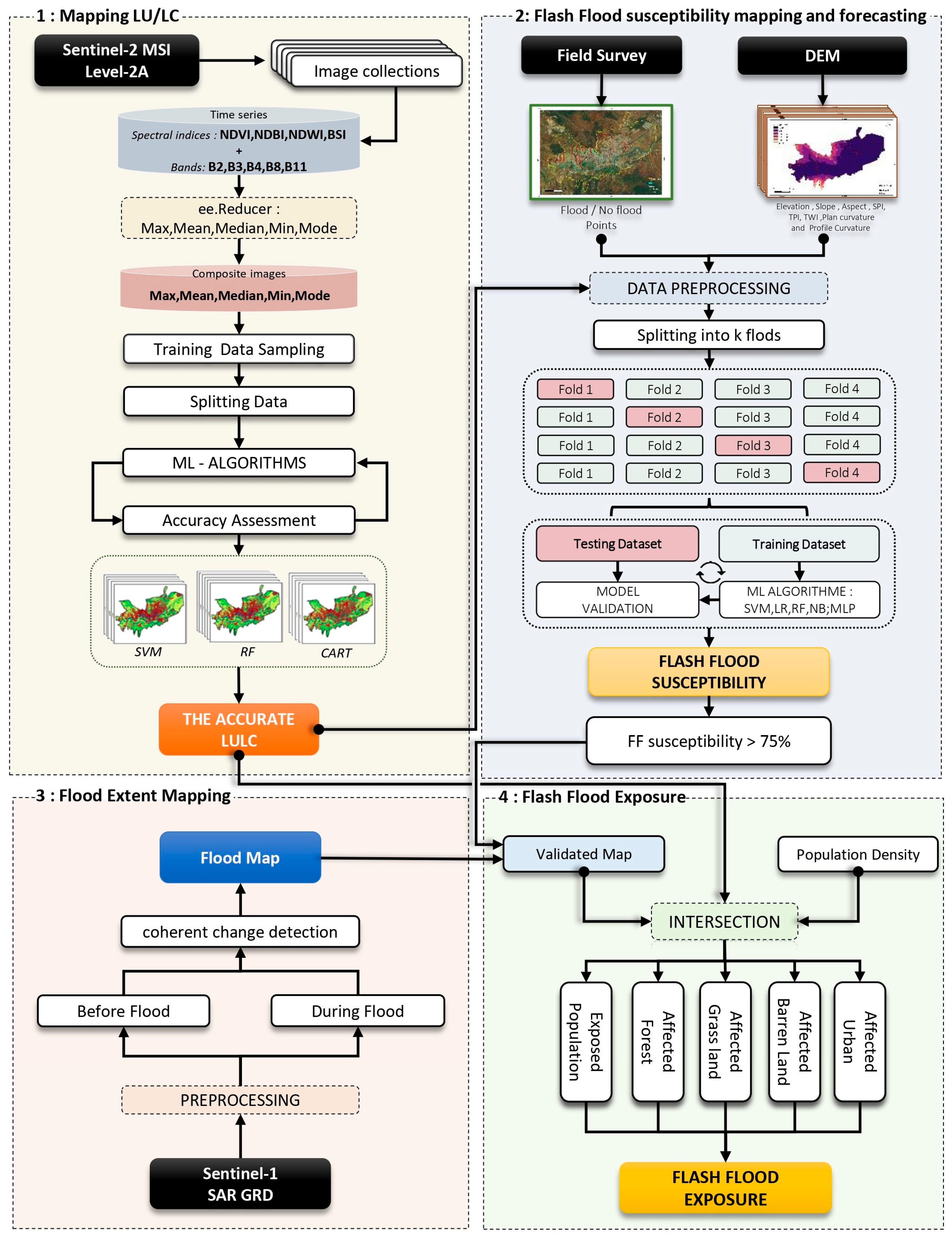
The following are the key components of the methodology used in this study: (1) Mapping of LULC with SENTINEL-2 MSI Level-2A. (2) Detection and prediction of FF susceptibility using a variety of factors. (3) Mapping of FF extent with Sentinel-1 SAR. (4) Determination of FF exposure in the region of interest based on LULC and population density. Figure 3 presents the methodology flowchart.

2.3.1. Mapping LULC

Accurate LULC mapping is crucial as it forms the basis for the rest of this study. A new approach was developed by comparing the results of five GEE-based composition methods to ultimately adopt the best one. Based on the literature, research employing GEE for LULC mapping and monitoring has grown significantly in recent years [32,33,34], with most of these studies comparing classifier performance while a few have compared findings from the same dataset using various compositions, including [23,35,36]. However, the methodology of our approach, which is completely built on the GEE cloud computing platform, began by selecting a collection of images of the S2 L2 sentinel (23 images) between March 1 and November 30 of 2021 (summer, autumn, and spring). For each image, the Normalized Difference Vegetation Index (NDVI) (Equation (1)), Normalized Difference Built-up Index (NDBI) (Equation (2)), Normalized Difference Water Index (NDWI) (Equation (3)), and Bare Soil Index (BSI) (Equation (4)) were calculated.

$$NDVI=\frac{B8-B4}{B8+B4}$$

(1)

$$NDBI=\frac{B11-B8}{B11+B8}$$

(2)

$$NDWI=\frac{B3-B8}{B3+B8}$$

(3)

$$BSI=\frac{\left(B4+B11\right)-\left(B8+B2\right)}{\left(B4+B1\right)+\left(B8+B2\right)}$$

(4)

where:

B2: Blue band

B3: Green band

B4: Red band

B8: Near-infrared band

B11: Short-wave infrared band

In this study, the focus was on the reduction operation, which can be used to obtain a significant array for high-dimensional inputs using specific aggregation functions [37], such as the calculation of the Max (the maximum pixel value of all linked bands), the Mean (the average value of each pixel), the Median (the middle number in the sequence (50th percentile)), the Min (the minimum pixel value), and the Mode (the highest pixel value). In this context, the integrated ee.Reducer function of GEE was used to combine the time series of spectral indices and create five composites (Max, Min, Mean, Median, and Mode) for each index. In addition, five other composites (Max, Min, Mean, Median, and Mode) were created based on bands (B2, B3, B4, and B8) with the same spatial resolution (10 m) (

Table 2. Composite images generated from image collections in the study area.

Reducer	Band	Resolution
ee.Reducer.max()	Blue (B2), Green (B3), Red (B4), NIR (B8)	10 m
ee.Reducer.min()	Blue (B2), Green (B3), Red (B4), NIR (B8)	10 m
ee.Reducer.median()	Blue (B2), Green (B3), Red (B4), NIR (B8)	10 m
ee.Reducer.min()	Blue (B2), Green (B3), Red (B4), NIR (B8)	10 m
ee.Reducer.mode()	Blue (B2), Green (B3), Red (B4), NIR (B8)	10 m
ee.Reducer.max()	NDVI, NDWI, NDBI, BSI
ee.Reducer.min()
ee.Reducer.median()		10 m
ee.Reducer.min()
ee.Reducer.mode()

). Bands B2, B3, B4, B8 NDVI, NDWI, NDBI, and BSI were concatenated according to the reducer used to form a dataset with 8 features used as predictor variables in the ML process. For example, the mean composite dataset contains B2_mean, B3_mean, B4_mean, B8_mean, NDVI_mean, NDWI_mean, NDBI_mean, and BDI_mean.

Numerous studies have shown that the integration of spectral indices can improve the accuracy of classification and the ability to differentiate between different forms of land cover [23,33,37]. By using specific features of the land surface, such as the amount of vegetation, built-up areas, water areas, and bare soil, these indices provide a more complete and accurate description of land cover.

The primary LULC in the research area is presented by five classes: barren land (BL), water (W), forest (F), vegetation (V), and urban (U). Visually interpreting high-resolution Google Earth images, 540 land polygon samples totaling 6147 pixels are determined using a random distribution in LULC categories (

Table 3. Training and validation data.

LULC	No. of Polygons	No. of Pixels	Training Pixels	Testing Pixels
Water	108	1852	1297	556
Bare Land	97	641	447	192
Green land	114	1174	822	353
Forest	105	1492	1045	448
Urban	116	988	693	296
SUM	540	6147	4304	1845

).

The datasets were split randomly into two groups: (1) 70% of the samples correspond to the training data that were employed to feed the machine learning algorithms. (2) The remaining samples (30%) comprising the testing samples have been used to assess the models’ capabilities using various metrics (Section 2.5).

2.3.2. Mapping and Forecasting of Flash Flood Susceptibility

The likelihood that a place or region can be affected by a FF is called FF susceptibility. It is determined by several factors (climatic, hydrological, and geographical). In this proposed method, we tried to estimate this susceptibility using five ML algorithms (Section 2.4) (RF, LR, SVM, MLP, and NB) based on 8 FF factors derived from the DEM (Topographic Position Index, Current Index, Profile Curvature, Topographic Wetness Index, Elevation, Plane Curvature, Aspect, and Slope), the exact LULC results from the first approach (Section 2.3.1) as independent variables, and the locations of flash flood and non-flash-flood areas as dependent variables. For each independent variable, the data were standardized using StandardScaler to ensure that each feature in a dataset had the same distribution or scale. Based on the previous literature, it may be difficult to select the most important factors as they differ from one study to another. Therefore, in our case, nine factors (topographic wetness index, LULC, profile curvature, topographic position index, current index, plan curvature, elevation, orientation, and slope) were selected based on the local characteristics of the study area. On the other hand, precipitation is a key factor for flooding but was not used in our study because we assumed that the same amount of precipitation is experienced throughout the city, which is a relatively small area. This concept is well confirmed by Shahabi’s study [38].

To ensure a reliable evaluation and minimize the effects of random data splitting, K-fold cross-validation was used, where K equals 4. In our case, this method divides the data iteratively into four folds (groups). In each iteration, three folds are used to form the model, with the last one being used for evaluation. To ensure that all data points are used for both training and testing, this process is repeated four times. The models were evaluated using various metrics averaged across the four folds of the K-Fold cross-validation procedure, including precision, F1 score, recall, accuracy, kappa index, and the receiver operating characteristic (ROC) curve.

The quality of the input data has a significant impact on the final results. For this reason, the data must be cleaned before use. One of the most effective approaches for this is the elimination of outliers, i.e., points that are indistinguishable from all or most other points [39]. Identifying and eliminating outliers is a difficult task as it is necessary to have a good understanding of the subject and the data collection process. The present study visually analyzes the data to identify outliers, using scatterplots and box plots to highlight the data and then eliminate observations that are too far from the actual cluster of observations. Although automated methods for removing outliers, such as the interquartile range (IQR) or z-scores, are valuable tools, they can sometimes have unexpected consequences. For example, in our study area using digital elevation model (DEM) data, we found that the highest elevation in our region is around 400 m, with only a few data points at this level. However, automatic outlier removal could wrongly label these points as anomalies because they exceed certain thresholds, whereas they represent genuine but less common features of the landscape. Removing them could distort our overall understanding. That is why we decided to take a different approach. Instead of using an automated method, we visually analyzed each factor and its statistical properties. This enabled us to identify and preserve relevant data points that might be mistakenly considered outliers by automated techniques.

Land Use Land Cover (LULC)

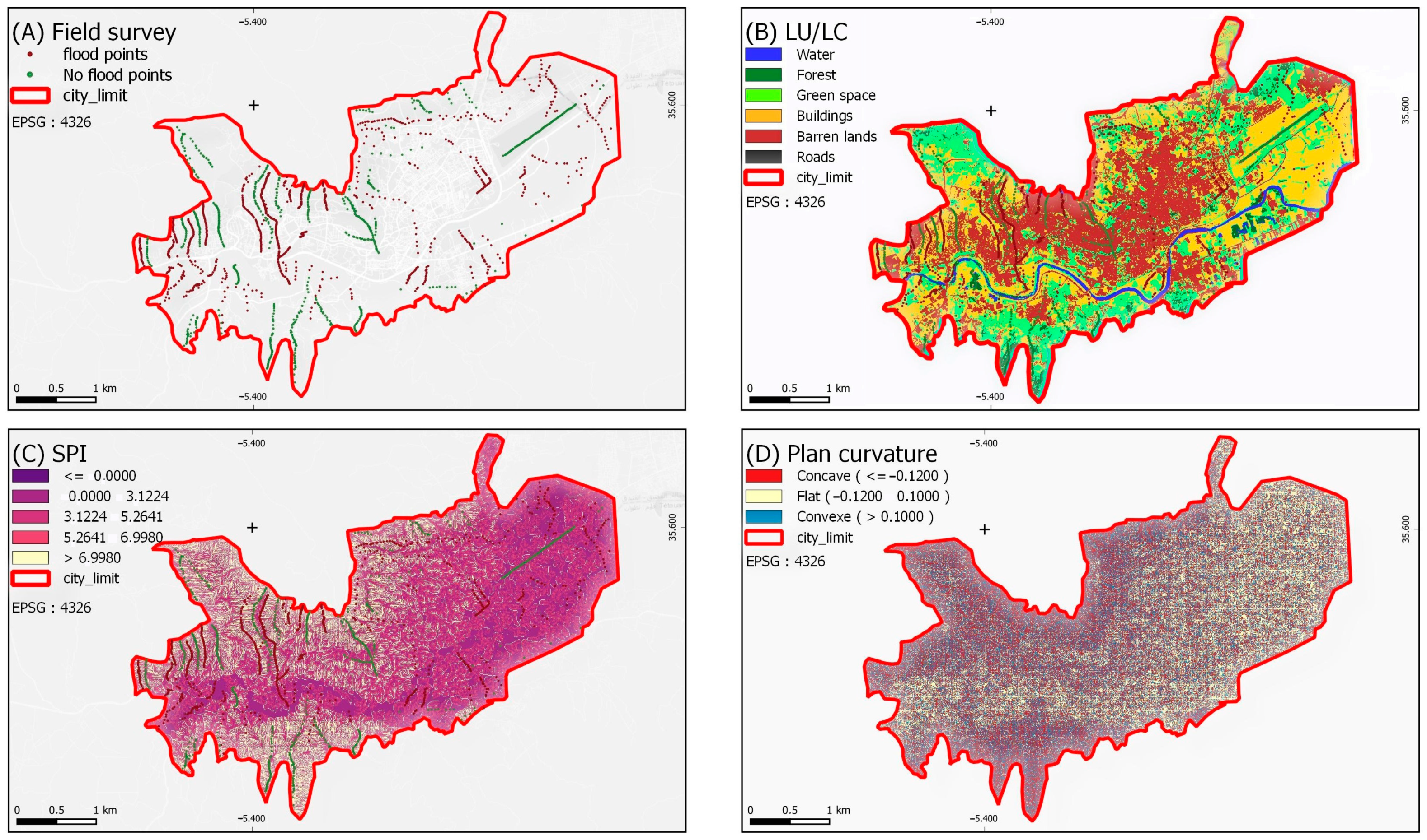
Section 2.3.1 provided a thorough explanation of the method used to create LULC. Five classes were established: 0 for Water, 1 for Bare Land, 2 for Vegetation, 3 for Forest, and 4 for Urban areas (Figure 4B), with a noticeable lack of forest regions, which greatly helps the water equilibrium at the watershed level, as well as a predominance of urban areas, which are known to strongly support flash flooding. The final resolution of the produced LULC raster is 10 m.

Stream Power Index (SPI)

The destructiveness of rushing water is measured by the Stream Power Index (SPI). In order to calculate the SPI, the catchment area (flow accumulation) and the slope are the basis of the calculation, following Equation (5). Figure 4C shows the SPI in a raster format with a 10 m resolution.

$$SPI= \alpha \times \tan \left(\beta \right)$$

(5)

where α: The catchment area, $\beta$: Slope.

Plan Curvature

One type of morphometric factor is plane curvature, which is used to delineate high- and low-runoff areas. Concave, flat, and convex results were the three classifications that were created using this factor. Using the Curvature tool in ArcGIS Pro and the output plan curve function, we were able to generate plan curvature values in raster format with a resolution of 10 m (Figure 4D).

Profile Curvature

An essential morphometric characteristic that identifies the region where runoff is increased is profile curvature. Positive numbers represent slower surface water flow, while negative values represent quicker surface water flow. We obtained profile curvature values in raster format with a resolution of 10 m using the output profile curve function in the Curvature tool of ArcGIS Pro software. Around 68% of the research area is covered by accelerated runoff surfaces (−0.17) (Figure 5A).

Topographic Position Index

The topographic Position Index is a morphometric factor that calculates the elevation difference between a specified cell and the average elevation inside a certain determined range (Equation (6)). Using the natural break method, the TPI values from this study were classified into five categories in a raster format with a resolution of 10 m (Figure 5B).

$$TPI=M_0-{{\displaystyle \sum }}_{n-1}^n{M}_n/n$$

(6)

where: $M_0$ = altitude at the center point

$M_n$ = grid elevation

n = Surrounding points

Topographic Wetness Index

The local equilibrium between slope and flow accumulation is presented numerically by the topographic wetness index (Figure 5C) (Equation (7)). The TPI produced in this study is a raster with a resolution of 10 m.

$$TWI=\ln \left(\frac{\alpha }{\tan \beta }\right)$$

(7)

where α: The catchment area, β: Slope.

Elevation

Any FF event may be impacted by elevation, which is the vertical distance from a point to the geoid or ellipsoid reference. Lowland areas are often more prone to flooding due to factors such as river overflow and gravity. In the case of FFs, certain areas, even at higher altitudes, can be more vulnerable to FFs due to the rapid accumulation of water caused by intense precipitation in higher areas. The study area’s elevation raster has a resolution of 10 m (Figure 5D).

Slope

The slope is calculated using the DEM and is regarded as a good control factor for water flow velocity. This is why it is taken into account, as it is one of the factors with the greatest impact on FFs. In this study, it has been divided into five clusters with a 10 m spatial resolution. As shown in Figure 5E, those categories whose values are under 11.08 predominate in the study area’s middle, while classes with values over 55.463 predominate in the study area’s upper and lower portions.

Aspect

The aspect is a morphological factor that presents the directional slope orientation that is derived from the DEM. Aspect subtly influences flash flooding. North-facing slopes may preserve their saturation longer, increasing runoff, whereas south-facing slopes dry out more quickly. A raster with ten classes and a resolution of 10 m is the end product used to present the aspect in our study (Figure 5F), where each pixel shows which way the surface is facing at that precise location. Given that flat areas do not have a downhill direction, the aspect’s direction is calculated on a clockwise basis from 0 to 360 degrees.

2.3.3. Flash Flood Extent Mapping

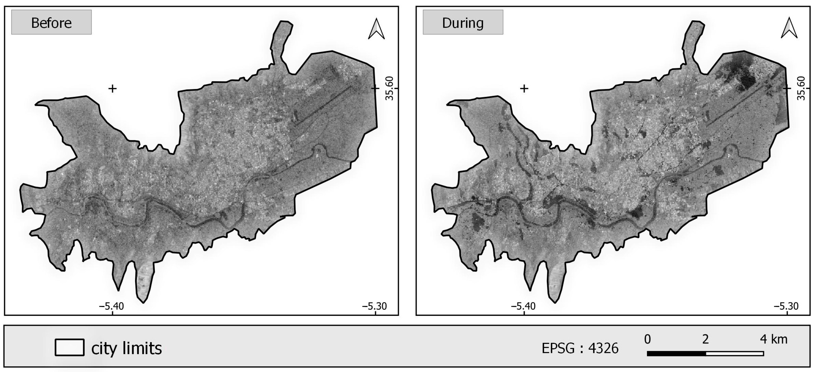
Based on the GEE environment, the extent of FFs was determined using Sentinel 1 SAR. This determination started by selecting the best images based on the FF’s date of occurrence (1 March 2021), then determining polarization, which was VV polarization. This proved more effective than VH polarization in our case, although it is considered more sensitive to vertical structures and it is beneficial to distinguish open water from the land surface, while VH polarization is more sensitive to surface changes. The direction of passage was also determined to avoid false positive signals caused by a different viewing angle. Given the location of our study area, the descending transit direction was chosen (based on the Sentinel 1 observation scenario). The following processing steps have already been applied to each Sentinel 1 SAR image: Terrain rectification, radiometric calibration, and thermal noise elimination. A speckle removal filter was then applied to reduce the speckle effect, which occurs in radar images and is perceived as a grainy appearance in images generated with a coherent imaging system [40]. Our method for detecting FF extent involved a simple change detection approach using an empirical threshold. First, a raster was created by dividing a “during-FF” mosaic image by a “before-FF” mosaic image (Figure 6). This process revealed areas where pixel values had changed significantly between the two images. Light pixels indicated significant changes, which could indicate FF regions, while dark pixels indicated minimal changes. To distinguish FF areas from other changes, a predetermined threshold of 1.06 was used. Pixel values below the threshold were set to 0, indicating no significant change, while pixel values above the threshold were assigned a value of 1, indicating probable FFs. This procedure resulted in a binary raster map illustrating the potential extent of FFs. It is worth noting that the selection of this threshold required a manual trial-and-error procedure to effectively capture the geomorphologic patterns associated with FFs in the specific study. In addition, the permanent water (extracted from LULC) was again removed to avoid false positives in FF extent. Finally, areas with a very high susceptibility to FF and field FF points were used to validate the results.

2.3.4. Damage Assessment—Flash Flood Exposure

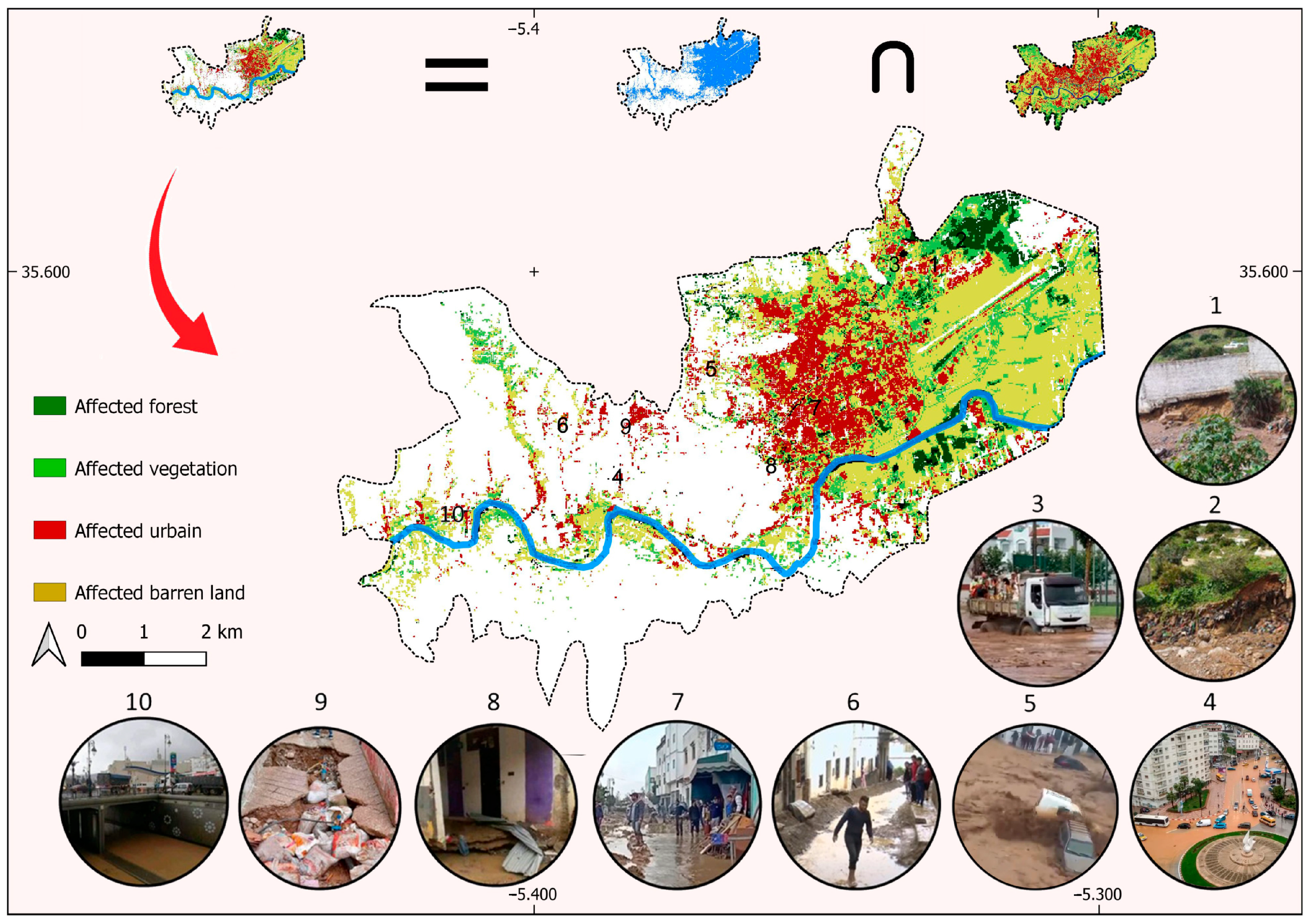
The LULC areas (barren, water, vegetation, forest, and urban) were intersected with the validated FF map to generate each affected group, which was then used to determine the areas affected by the event and assess the damage. Additionally, the population density map was also intersected with the FF map to determine the exposed population density.

2.4. Machine Learning Algorithms

Unsupervised learning, supervised learning, and reinforcement learning represent the three main categories of machine learning. Supervised learning entails using labeled data to train the model where the desired result is known. Finding patterns and connections between variables in unlabeled data is the goal of unsupervised learning. Machine learning is trained to interact with an environment to maximize reward through reinforcement learning. The principal supervised algorithms suggested in this research are RF, NB, SVM, MLP, LR, and CART.

2.4.1. Support Vector Machine (SVM)

SVM is considered a widespread algorithm in the machine learning field; it is considered to be a supervised method aimed at classification and regression problems. The SVM determines the best function for predicting the output variable based on the input variables, or the best hyperplane to divide the input data into distinct classes. It handles this by determining the largest margin from the hyperplane(s) to the closest data points in a given class, making it less vulnerable to noisy or overlapping data [41].

2.4.2. Logistic Regression (LR)

A supervised learning algorithm called logistic regression (LR) is used for binary classification, where the input and output variables may be continuous or categorical. It maps any input to output between 0 and 1 using a sigmoidal function to represent the connection between the predictor variables and the probability of the response variable [42].

2.4.3. Random Forest (RF)

A particular supervised learning algorithm called the Random Forest (RF) works by constructing a multitude of hierarchical classifiers {h (, ${\theta }_k), k=1, \dots$}, in which the $\left\{{\theta }_k\right\}$ are independent, distributed, and identically random vectors, knowing that for a specific input x, each tree in the random forest model assigns a vote for the most prevalent class [43]. RF is renowned for its ease of configuration, making it relatively easy to adjust for optimum performance [44].

2.4.4. Naïve Bayes (NB)

Based on the Bayes theorem, Naive Bayes (NB) is a probabilistic method for supervised learning, which is a mathematical framework for calculating probabilities. The name “naive” refers to NB’s assumption that the input features are independent of one another [45].

2.4.5. Multilayer Perceptron (MLP)

An essential part of Artificial Neural Networks (ANNs), a computing paradigm modeled after the architecture and operations of the human brain is the Multilayer Perceptron. The MLP network is made up of hidden layers connected by weighted neural connections and input layers that receive the variables utilized in the analysis. These hidden layers record complex links between the input and output layers. They are further related to the output layers through connections that carry output weights. The MLP uses a supervised learning method known as backpropagation to modify these weights during training with labeled data. The MLP may learn from the data through this iterative process, which enhances its capacity to carry out tasks such as function approximation and pattern recognition [46].

2.4.6. Classification and Regression Trees (CART)

The basic method of decision-making used by CART and RF is identical [36]. RF employs an ensemble, whereas CART utilizes a single tree. Based on predetermined thresholds, CART separates nodes recursively until they reach terminal nodes, also known as leaf nodes. By dividing the data effectively, these splits allow for iterative refinement of the decision limits. CART’s performance and adaptability are improved by this recursive process, which lets it customize the decision tree to the dataset.

2.4.7. Hyperparameters of Machine Learning Models

Precise parameter adjustments are typically required to enhance the performance of ML models. In this stage, we concentrated on tuning model parameters to earn increased precision. Each algorithm was tuned to determine the ideal set of parameters. This required modifying parameters such as tree depths, regularization terms, and learning rates. To achieve an equilibrium between model complexity and generalization capacity, we experimented iteratively and employed cross-validation, which guaranteed that the data were robust and accurately identified patterns.

Table 4. Hyperparameters of Machine Learning Models.

Phase	Algorithm	Best Parameters
LULC Mapping	RF	n_estimators = 14
	SVM	kernel = “linear”, Cost = 0.1
	CART	maxNodes: (50)
FF Susceptibility	SVM	kernel = “rbf”,C = 20
	RF	n_estimators = 200,
	LR	The same accuracy for all solvers: ‘newton-cg’, ‘lbfgs’, ‘liblinear’, ‘sag’, ‘saga’
	NB	var_smoothing: 1.000 × 10−9
	MLP	Hidden_layer_sizes = (15, 15), learning_rate_init = 0.01, mlp.out_activation_ = ‘sigmoid’

contains specific model parameters for each algorithm that we employed in our investigation.

2.5. Accuracy Assessment

Assessment is a crucial phase when using machine learning techniques because it helps identify model faults and limitations and determines whether it is overfitting (when an algorithm performs effectively while trained but fails when evaluated) or underfitting (when the model performs weakly across the testing and training datasets). Moreover, if there are several models, it can assist us in selecting the one that works best with the given data set. The evaluation can also assist in determining the generalizability of new data. Motivated by the latter reasons, this study used a variety of metrics to assess the different models used, namely the binary classification’s accuracy assessment and the multiclass classification’s accuracy assessment.

2.5.1. Binary Classification’s Accuracy Assessment

The process of assessing a classifier’s performance in separating between two classes using binary classification is known as binary classification accuracy assessment. When one category reflects a positive outcome while the other represents the negative case, the concepts of true negative (TN), true positive (TP), false positive (FP), and false negative (FN) are applied. Knowing that TP is used when a positive estimate coincides with the positive real worth, FN is used when a positive estimated value does not coincide with the actual positive value and gives a negative value. FN is used when an estimated number that is negative is different from the real value, which is negative and produces a positive, and TN is used when a negative predicted value is different from the actual negative value (

Table 5. Example of a binary confusion matrix.

		Actual
		Positive	Negative
Predicted	Positive	True Positive	False Positive
	Negative	False Negative	True Negative

).

Based on this concept, several metrics, including precision (Equation (8)), accuracy (Equation (9)), recall or sensitivity (Equation (10)), specificity (Equation (11)), F1 Score (Equation (12)), kappa index (Equation (13)), and the Receiver Operating Characteristic Curve, can be derived.

$$Precision=\frac{TP}{TP+FP}$$

(8)

$$Accuracy=\frac{TP+TN}{TP+FP+FN+TN}$$

(9)

$$Recall or Sensitivity=\frac{TP}{TP+FN}$$

(10)

$$Specificity=\frac{TN}{TN+FP}$$

(11)

$$F1 Score=\frac{2\times Precision\times Recall}{Precision+Recall}$$

(12)

$$Kappa=\frac{Accuracy-\mathrm{Chance} \mathrm{Agreement} \left(\mathrm{Pe}\right)}{1-\mathrm{Chance} \mathrm{Agreement} \left(\mathrm{Pe}\right)}$$

(13)

$$\mathrm{Chance} \mathrm{Agreement} \left(\mathrm{Pe}\right)=(p_1\times p_{1.pred})+\left(p_2\times p_{2.pred}\right)$$

(14)

where:

TP = true positive

FP = false positive

TN = true negative

FN = false negative

$p_1$ = the proportion of instances in the true labels in class one.

$p_{1.pred}$= the percentage of predicted instances in class one.

$p_2$ = the proportion of instances in the true labels in class two.

$p_{2.pred}$ = the percentage of predicted instances in class two.

The Receiver Operating Characteristic (ROC) Curve represents the graphical representation of the true positive rate (TPR) (sensitivity) versus the false positive rate (FPR) (specificity) for various limits or thresholds such as 0.1, 0.2, 0.3, and 0.9 [47]. It is not a mathematical formula but rather a plot of the performance of a binary classification where the x-axis and the y-axis, which stand for the FPR and TPR, respectively, can be used to visually depict the ROC curve. Furthermore, the ROC curve was obtained by tracing various classification thresholds from point (0,0) to point (1,1), starting with the first classification threshold. A random classifier is represented by a diagonal line (a chance line) from (0,0) to (1,1), and the closer the ROC curve is to the point (0,1), the more efficiently the classifier performs overall. A frequently used statistic for evaluating the performance of models is the area under the ROC curve (AUC), with an ideal model having an AUC of 1 and a random classifier having an AUC of 0.5.

2.5.2. Multiclass Classification’s Accuracy Assessment

Assigning the inputs to one of numerous predefined classes is the goal of the machine learning task known as multiclass classification, also referred to as multinomial classification. The algorithm must predict more than two potential classes in this kind of classification. Assessment of a multiclass classification needs a representation of the predicted class labels against the true class labels that show the number of instances that are correctly classified and misclassified for each class.

To evaluate a multiclass classification, the instances correctly and incorrectly classified for each category must be displayed in a very well-organized tabular representation called a confusion matrix of the predicted class labels against the actual class labels (

Table 6. Four classes (A, B, C, and D) are used as examples of a confusion matrix, with Kappa = 0.817 and OA = 0.863.

		Actual
		A	B	C	D	Sum	UA
predicted	A	107	2	7	10	126	0.8492
	B	1	80	5	3	89	0.8989
	C	4	11	100	6	121	0.8264
	D	3	2	7	98	110	0.8909
	Sum	115	95	119	117
	PA	0.9304	0.8421	0.8403	0.8376

). The classification product and associated validation sample can be cross-tabulated to determine a variety of metrics, such as overall accuracy (15), class producers’ accuracy (16), class users’ accuracy (17), and kappa statistic (18).

$$\mathrm{Overall} \mathrm{Accuracy} \left(\mathrm{OA}\right)=\frac{Number of correctly classified samples}{Number of total samples}$$

(15)

$$\mathrm{class} \mathrm{Producers}\text{’} \mathrm{Accuracy} \left(\mathrm{PA}\right)=\frac{Nnumber of samples in each class correctly classified.}{Number of samples from reference data in each class}$$

(16)

$$\mathrm{class} \mathrm{User}\text{’}\mathrm{s} \mathrm{Accuracy} \left(\mathrm{UA}\right)=\frac{number of samples in each class correctly classified.}{Number of classified samples to that class}$$

(17)

$$\mathrm{Kappa} \mathrm{statistic}=\frac{OA-\mathrm{Expected} \mathrm{Agreement} \left(\mathrm{Pe}\right)}{1-\mathrm{Expected} \mathrm{Agreement} \left(\mathrm{Pe}\right)}$$

(18)

$$\mathrm{Expected} \mathrm{Agreement} \left(\mathrm{Pe}\right)=\frac{\sum \left(row totals in each class\times column total in each class\right)}{{\left(Number of total samples\right)}^2}$$

(19)

3. Results

The methodology described above has led to four levels of results: (1) LULC; (2) FF susceptibility; (3) FF areas; and (4) FF exposure.

3.1. Land Use Land Cover (LULC)

It was difficult to select the ideal LULC for the research area; therefore, it was necessary to compare several methods. The statistical functions mode, min, median, mean, and max were used to create five composites, which were then classified using SVM, RF, and CART. Three classification maps were created for each composite based on the algorithm used. A total of fifteen maps were created (Figure 7). Each map includes five classes (water, wasteland, grassland, forests, and urban areas).

Comparing the performance of the three algorithms used (CART, RF, and SVM) reveals that SVM performs best when classifying Max, Mean, and Median composites (Max: OA = 87.87%, Kappa = 84.81%; Mean: OA = 95.97%, Kappa = 94.59%; Median: OA = 93.01%, Kappa = 91.6%), followed by RF (Max: OA = 87.39%, Kappa = 84.23%; Mean: OA = 92.84%, Kappa = 89.56%; Median: OA = 92%, Kappa = 90.85%) and then CART (Max: OA = 81.52%, Kappa = 76.89%; Mean: OA = 86.91%, Kappa = 83.01%; Median: OA = 90.02%, Kappa = 87.93%). However, when using Min and Mode composites, SVM performs poorly and is categorized as the worst result (Min: OA = 71.13%, Kappa = 68.8%, Mode: OA = 62.46%, Kappa = 58.98%), while RF and CART are categorized as the best result (Min: OA = 85.79%, Kappa = 82.17%, Mode: OA = 75.52%, Kappa = 69.21%) and the second-best (Min: OA = 82.51%, Kappa = 78.06%, Mode: OA = 69.55%, Kappa = 61.7%), respectively (Figure 8). In addition, the comparison of the most effective composites for LULC mapping (Figure 8) revealed that the average kappa (avg.Kappa) and average overall accuracy (avg.OA) were highest for the mean composite (avg.OA: 91.91%, avg.Kappa: 89.05%), followed by the median composite (avg.OA = 91.67%, avg.Kappa: 90.12%), the max composite (avg.OA = 85.59%, avg.Kappa = 81.97%), the min composite (avg.OA = 79.81%, avg.Kappa = 76.3%), and finally the Mode composite (avg.OA: 69.17% and avg.Kappa: 63.29%).

For each composite, the consumer accuracy (CA) and producer accuracy (PA) are determined for further investigations. The water class has the greatest CA and PA, followed by the urban class, forest class, grassland, and barren land, according to a comparison of the classifiers used (RF, SVM, and ANN) for all composites (

Table 7. Results of each LULC’s class-level accuracy assessment.

		Water			Barre Land			Greenland			Forest			Urban
		SVM	RF	CART	SVM	RF	CART	SVM	RF	CART	SVM	RF	CART	SVM	RF	CART
Max	UA	0.97	0.99	0.96	1	0.96	0.66	0.64	0.77	0.72	0.80	0.80	0.73	0.94	0.92	0.87
	PA	0.91	0.94	0.89	0.89	0.8	0.75	0.66	0.84	0.66	0.94	0.74	0.74	0.98	0.92	0.81
Mean	UA	0.99	0.96	0.96	0.79	0.92	0.8	0.95	0.87	0.89	0.93	0.8	0.76	1	0.99	0.98
	PA	1	0.96	0.92	1	0.91	0.91	0.87	0.86	0.82	0.9	0.83	0.87	0.98	0.95	0.95
Median	UA	0.95	0.98	0.96	0.97	0.87	0.75	0.89	0.76	0.9	0.69	0.81	0.79	1	0.96	0.93
	PA	0.96	0.93	0.9	1	0.85	0.74	0.72	0.8	0.87	0.8	0.95	0.87	0.97	0.95	0.93
Min	UA	0.98	0.9	0.91	0.63	0.89	0.57	0.62	0.72	0.73	0.77	0.88	0.86	0.98	0.93	0.89
	PA	1	0.96	0.98	0.8	0.41	0.68	0.69	0.85	0.65	0.68	0.79	0.83	1	0.99	0.78
Mode	UA	0.99	0.94	0.96	0.27	0.52	0.28	0.49	0.72	0.63	0.89	0.77	0.68	0.93	0.82	0.83
	PA	0.99	0.94	0.92	0.58	0.37	0.4	0.62	0.72	0.53	0.68	0.87	0.75	0.7	0.87	0.78
	Avg UA	0.98	0.95	0.95	0.73	0.83	0.61	0.72	0.77	0.77	0.82	0.81	0.77	0.97	0.92	0.90
	Avg PA	0.97	0.95	0.92	0.85	0.67	0.70	0.71	0.81	0.71	0.80	0.84	0.81	0.93	0.94	0.85

). It is also hereby informed that the accuracy of consumers and producers in all LULC categories is higher when the mean composite image generated by SVM is used. Since the map generated by the SVM algorithm based on the mean composite image was the most accurate among the numerous evaluation metrics, we decided to use it for the next phases of our investigation.

3.2. Flash Flood Susceptibility

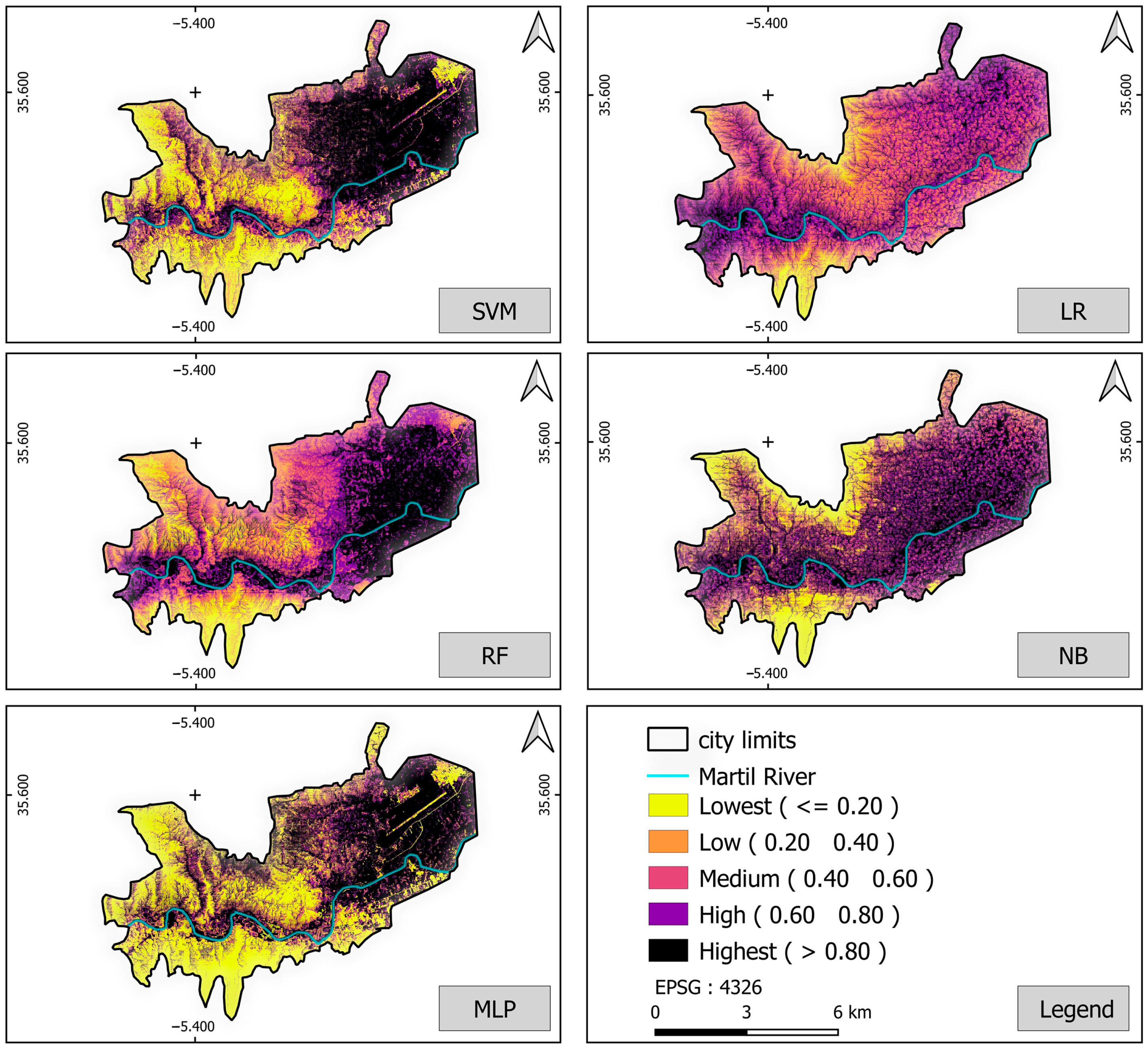
Figure 9 shows FF susceptibility maps generated by five ML algorithms (RF, SVM, NB, MLP, and LR). Five levels of susceptibility are shown on each map: highest, high, moderate, low, and lowest. The high susceptibility areas are mainly located in the southeastern part and along the Oued Martil river, which can be seen on each map. This was supported by the morphology of the city, which resembles a basin between two mountains (north and south), in such a way that the water accumulates in the middle along the river. The high susceptibility of the eastern region of the city is also reflected in the fact that the slope runs from west to east.

The SVM model predicted that 31% of the area was at the highest FF risk, followed by 21% at high FF risk, 20% at the lowest FF risk, 18% at moderate FF risk, and 10% at low FF risk. In contrast, the LR model showed that 39% of the study area was at high FF risk, 19% was at moderate FF risk, 19% was at low FF risk, and 23% was at the lowest FF risk. Similarly, for the RF model, 37% of the area under study is at the highest FF risk, 18% of the FF risk is high, 19% presents a moderate FF risk, 13% has a low FF risk, and 13% has the lowest FF risk. On the other hand, the NB model estimated that 44% of the study area was at highest FF risk, 14% at high FF risk, 10% at moderate FF risk, 15% at low FF risk, and 17% at lowest FF risk. Finally, the ANN model predicts a 31% high FF risk area, a 17% high FF risk area, a 13% moderate FF risk area, a 15% low FF risk area, and a 24% lowest FF risk area.

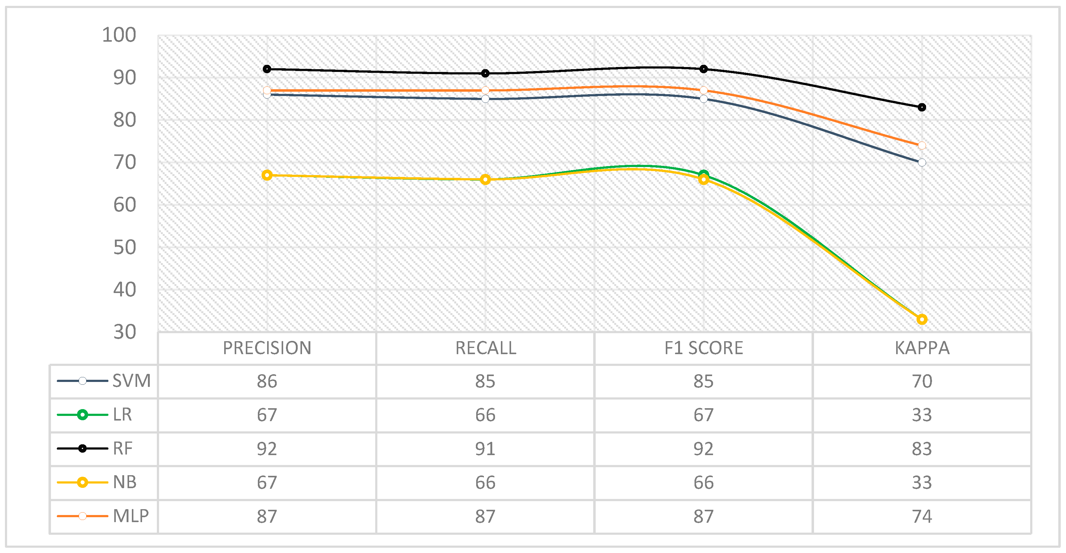
Based on the performance of the five algorithms used (Figure 10), RF performed best (recall: 91%, precision: 92%, Kappa statistics: 83%), followed by MLP (recall: 87%, precision: 87%, Kappa statistics: 74%), then SVM (recall: 85%, precision: 86%, Kappa statistics: 70%), LR (recall: 67%, precision: 66%, Kappa statistics: 33%), and finally NB (recall: 66%, precision: 67%, Kappa statistics: 33%). The model’s reliability was also evaluated using the AUC (Figure 11). AUC values for LR, NB, SVM, MLP, and RF are, respectively, 0.73, 0.73, 0.86, 0.93, and 0.97. All of these methods of assessment demonstrate that the RF algorithm is the most effective for detecting FF susceptibility in our area of interest.

To thoroughly comprehend each of our variables and examine the connections between them, Figure 12 shows the Pearson’s correlations that were revealed. Pearson’s correlation coefficient is between −1 and 1, with 1 indicating a perfect positive correlation, a value of −1 indicating a perfectly negative correlation, and a value of 0 indicating that there is no correlation. In our case, correlation coefficients range from −0.68 to 0.72.

The correlation matrix (Figure 12) revealed significant relationships between the variables. Strong correlations (>0.7 or <−0.7) were observed between TPI and plan curvature (−0.68), slope and DEM (0.71), TWI and FF occurrence (0.71), and FF occurrence and DEM (−0.68). Moderate correlations (0.4 to 0.7 or −0.4 to −0.7) were observed between TWI and slope (−0.4), FF occurrence and TPI (0.4), FF occurrence and slope (0.5), TWI and DEM (−0.31), and plan curvature and profile curvature (−0.6). Weak correlations (<0.4 or >−0.4) were observed between LULC and all variables and SPI and most variables.

Based on the RF algorithm, elevation is identified as a key factor influencing the occurrence of FFs, followed by position (Y,X), slope, LULC, SPI, aspect, TWI, plan curvature, TPI, and profile curvature. For the MLP, position on the Y-axis and elevation are the most important variables for FF susceptibility, followed by X-position, TWI, aspect, LULC, slope, SPI, TPI, plan curvature, and profile curvature (Figure 13).

3.3. Flash-Flooded Areas

Another way of extracting flash-flooded areas has been achieved using SAR data. The locations of FF zones extracted from SAR data are clearly shown in Figure 14. Analysis of Figure 14 shows a high concentration of FF zones, particularly in the eastern part of the study area and along the Martil River.

This spatial distribution (Figure 14) corresponds closely to the locations identified during the FF points field surveys, particularly along the Martil River and in the eastern sector. The black rectangle in Figure 14 highlights an area where FF detection by Synthetic Aperture Radar (SAR) is limited due to its 10 m spatial resolution. This limitation is to be expected, particularly in metropolitan areas characterized by densely populated neighborhoods and narrow roads. The inability of SAR to detect FF zones in these urbanized areas underlines the importance of complementary data sources and the need for localized monitoring strategies to effectively identify and mitigate FF risks in urban areas.

This limitation is further underlined by the results of the ML algorithm obtained in the previous section, which successfully identified areas with a high FF susceptibility (>75%).

However, basing our analysis only on SAR data may have led to an underestimation of the total potential for FF in urban areas due to its limited resolution to capture features such as small buildings and small streets. For this reason, an overlay between the two results (FF-SAR DATA and FF susceptibility) was used to gain an in-depth overview of FFs in the study area. This overlay (Figure 15) confirmed and validated these results, with a compliance score of 80%.

3.4. Flash Flood Exposure

To determine exposure, we integrated various data sets, including SAR data, high FF susceptibility (>75%), and field survey points (FF and non-FF points).

The degree of susceptibility of people, buildings, or systems to potential risks or hazards is referred to as exposure. Visualization of SAR data can be used to identify potentially FF-prone areas, although its effectiveness in urban environments is limited. The identification of areas with high FF susceptibility (>75%) allows the localization of areas at high risk of flash floods, which requires special attention in terms of emergency preparedness, infrastructure planning, and land use management to limit potential damages. In addition, the overlay of field survey points enables exposure assessments to be validated and improved by incorporating field data, thus increasing the accuracy and reliability of this approach. By overlaying these three results with LULC and population data, we identified the land use types that are most likely to be exposed and extracted the exposed population. It is important to note that areas with false positive results indicating the presence of FFs were filtered out and excluded. By accurately extracting data on the actual risk of FF, this process ensures that emergency preparedness plans and risk reduction initiatives are targeted accordingly. Using the GEE platform, FF exposure was determined and displayed on a user interface (Figure 16), which provides a global view of the exposure situation with estimated values for each affected section and the possibility to click on any part of the map to obtain information on whether the clicked point is flooded or not.

Figure 17 clearly illustrates part of this exposure, namely the number of people exposed to population density. A total of 198,913 inhabitants have been exposed. For LULC, the affected areas were also extracted (Figure 18), with 2465 hectares affected (513 hectares of affected vegetation, 582 hectares of affected urban areas, 1213 hectares of affected barren areas, and 157 hectares of affected forest areas). The results obtained were validated in the field (Figure 18).

4. Discussion

Over the past three years, Tetouan has been confronted with numerous FFs, with an average of one per year, causing major damage. This prompted us to try to understand and map the pattern of these FFs, taking the FF of 2021 as an example. Our main objective was to assess the damage during and after the event using remotely available data and utilizing a cloud computing platform (GEE) enhanced with ML algorithms.

Based on the initial results of this study, the effectiveness of the proposed methodology has been well demonstrated; however, the limitations and possible sources of uncertainty need to be addressed.

The first result obtained in this study is LULC. In that section, we aimed to evaluate several composites (Min, Max, Median, Mode, and Min) using three ML algorithms (SVM, RF, and NB) to determine those that can be used for the rest of our study. This assessment was based on Sentinel-2 imagery rather than Landsat imagery as the latter has been used by most researchers when using GEE [48,49]. Our decision was influenced by the study area’s morphology, which is made up of small condensed districts, and also by the diversity of land classes, which requires good spatial resolution (10 m in Sentinel 2 instead of 30 m in Landsat).

The fifteen maps produced were compared (Figure 7). This comparison in terms of OA and Kappa index gave us reasonable results, according to the USGS and Gashaw et al. [50], who recommended accuracies of 85% and 80%, respectively. The best classification threshold in our case was that of SVM; it performed best for all composites (except the Min composite). The results were confirmed by many researchers who chose to use SVM to map LULC [51,52,53]. Our approach was not only about identifying the best classifiers but also about testing performance based on multiple composites. All composites created in our study are based on a collection of images from three seasons (summer, autumn, and spring). We excluded the winter season due to the large number of clouds. A comparison between the composites used also leads to the conclusion that the mean composite performed best out of all classifiers. This was confirmed by visual interpretation and can be explained by the fact that using a mean composite reduces temporal variations and atmospheric noise by taking the mean while also mitigating the effects of cloud cover. Nevertheless, the mean composite has a weakness in some cases as it is influenced by outliers. Therefore, in the literature, we have found that some authors use the median instead of the mean [23,54,55]. The choice of the best composite between median and mean depends entirely on the morphology of the area studied, the data specificity, and the LULC generation objective. We have chosen to use a mean composite classified by SVM for the remainder of our study, but it should be mentioned that, despite the accuracy of the results obtained, they could be improved by introducing other topographical factors into the training part of our models, which has proved their effectiveness in several studies [21,34,56].

The second result generated is the FF susceptibility. For this purpose and to obtain an accurate result, we trained our models based on five ML algorithms (SVM, LR, LR, RF, NB, and MLP), with the conclusion that RF is the best classifier, which corresponds to previous studies [57,58,59]. Therefore, we trained all our algorithms based on nine factors (topographic wetness index, LULC, profile curvature, topographic index, stream power index, plan curvature, elevation, aspect, and slope). Most studies with the same objective as ours have introduced rainfall as a factor directly influencing flooding [60,61,62,63]. Still, in our study, we neglected it because our region of interest is small and the same amount of precipitation is found all around it, so rainfall will have the same effect at any point in the region. This fact has been confirmed by numerous studies, of which the study by Shahabi et al. [38] is the best example. Rainfall was introduced as a factor in the first part of the study but ultimately, it was confirmed that the relationship between rainfall and flooding is more complex than a simple correlation between the quantity of rainfall and flood intensity.

Based on the Pearson correlation analysis presented in Figure 12, it is possible to understand the strength of the relationships between the different variables. In terms of TPI and plan curvature, TPI measures the relative elevation of a point while PC assesses the relative curvature of the terrain in the direction of the slope. Since higher elevations tend to have less curvature, it is logical that TPI and PC have a strong negative correlation. Concerning slope and DEM, areas with higher DEM values tend to have steeper slopes, which explains the strong positive correlation between these two variables. In the same way, TWI and FF occurrence show a strong positive correlation because areas with higher TWI values are more likely to experience flooding, while areas at lower elevations are more vulnerable to flooding, which explains the strong negative correlation between FF occurrence and DEM. Regarding TWI and slope, wetter areas are more likely to have flatter terrain, resulting in a moderate negative correlation between TWI and slope. TWI and DEM have a moderate negative correlation, as higher DEM values (higher elevations) tend to be drier, with water flowing downhill towards lower elevations. Plane curvature and profile curvature measure opposite aspects of the surface’s curvature. Therefore, it is logical that they have a moderately negative correlation. Lower TPI values and steeper slopes are linked to higher FF risk. This is because lower TPI values indicate lower elevations and steeper slopes create more runoff, possibly leading to flooding. LULC and the other variables in the dataset are not directly related to each other. For example, a change in LULC does not necessarily lead to a change in SPI, DEM, TPI, plan, or profile. This explains the weak correlations between LULC and all variables. Finally, SPI is a measure of a stream’s erosive power over time, while the other variables in the dataset are measures of various environmental characteristics at a specific location. This explains the relatively weak correlations between SPI and most variables. It should be noted that the previous studies did not all use the same variables; rather, different variables were used in each study. In essence, the decision depends on the morphology of the study area and the nature of the event; in fact, there is no precise consensus regarding the factors that must be taken into account, but in general, it is preferable to use more than six factors to minimize the production of reflective weights that are influenced by a single weight, leading to an overestimation of certain factors responsible for flooding [64].

Instead of the previous result, which gives an overview of the basic variables that influence the occurrence of the event at each location with the degree of susceptibility to FFs, we needed to closely monitor FFs before and after to determine the extent and severity, and this was achieved by using Sentinel-1A SAR GRD data, which are considered a powerful backup that provides useful information for FF monitoring both during the day and at night, regardless of cloud cover. However, despite these advantages, it is not always possible to use these data due to their temporal resolution, which is usually 6–12 days, depending on where you are. This temporal resolution may not be sufficient to track the progression of flooding as the water changes rapidly. In addition, the spatial resolution of 10 m is not enough to determine the true FF extent in the small streets and neighborhoods, as was the case in the Old Town in our region. Our result was validated using high FF susceptibility and the field survey points with an accepted score.

The final level of analysis in our study was to determine exposure. The difficulty lies in the accuracy of the results we had to use: for LULC, we used the best results of the first outcome (Section 3.3), for FF susceptibility, we used the precise result of the high-accuracy algorithm (Section 3.3), and for the FF extent, we used the SAR data (Section 3.4). To this end, we integrated these different data sets as well as field monitoring points (FF and non-FF points). The SAR data were used to identify potentially FF-prone areas, although their effectiveness in urban environments is limited. The identification of areas with high FF susceptibility (>75%) was used to localize areas at high risk of FFs. In addition, the overlay of field survey points was used to validate and improve exposure results. By overlaying these three results with LULC and population data, we were able to identify the types of land use likely to be exposed and extract the exposed population. It is important to note that areas with false positive results indicating the existence of FFs were filtered out and excluded. This procedure ensures that disaster preparedness strategies and mitigation measures are effectively targeted through the accurate extraction of data relating to actual FFs. The results of the intersectional study show that the region is located in a high disaster-risk zone and that rapid action is needed to limit the impact of the impending FF on people’s lives and economic situations.

Despite the high degree of accuracy achieved in our study, a visual interpretation of the final products shows some irregularities in certain areas, particularly those located in the condensed districts. This prompts us to think systematically about how to improve our final result. After analyzing our dataset, we concluded that improvements at this level are not possible, as all datasets used in our study are open-availability datasets with a 10 m spatial resolution. Therefore, advancements can be made in future research by using the same methodology, which has proven effective despite the use of low-resolution open data, but this time with commercial satellite data with high spatial resolution, such as data from Maxar (during major fatal natural disaster cases, it is often offered free of charge), Planet Labs, and Airbus Defense, or with government satellite imagery, as in the case of our study area, with the Moroccan satellites Mohammed 6 A and B. The latest commercial datasets proposed can be very important for accurate LULC mapping, with a spatial resolution of up to 30 cm. For DEM generation and FF mapping, we propose to use data from commercial SAR satellites, such as the Terra SARX radar satellite, with a spatial resolution of up to 25 cm. Furthermore, the use of LIDAR data is strongly advocated, and various studies have demonstrated their utility, particularly since the data can capture extreme features of a terrain [65], which may help in the production of very accurate DEMs and therefore increase modeling accuracy. Another effective method is the use of UAVs (unmanned aerial vehicles) equipped with sensors that differ according to the type of use. This is also considered an effective method of pre- and post-event monitoring and has proven its worth in numerous disasters.

Faced with the explosion of the population in all of the cities in the world, climate change, and an increase in disasters, we are faced with the challenge of reducing disasters; in fact, we cannot stop them, but we can reduce their effect, and it is time for all management strategies to take resilience into account and try to make the city resilient to disasters. Resilience is not about stopping disasters from occurring but rather about reducing their impact.

5. Conclusions

The current in-depth study offers insight into a cutting-edge method for mapping and detecting FFs using a combined approach of GIS techniques and machine learning within the GEE platform. To assess the damage in the study area, the proposed approach began by mapping LULC, determining susceptibility to FF, identifying the areas that were flooded, and determining FF exposure. The results obtained demonstrate the effectiveness of the methodology used, with the conclusion that the region falls within a high-risk hazard area and that immediate action is needed to lessen the effects of impending FFs on people’s livelihoods and economic conditions. Overall, the study offers insightful information about Tetouan’s FF problems that can be used to create mitigation plans that will lessen FF susceptibility in the future. The use of openly available datasets with low spatial resolution placed restrictions on the study. Future research could use higher-resolution commercial satellite data to increase the accuracy of the findings. The effect of climate change on FFs was not taken into account in the study. Future research should take this into account to create more effective mitigation measures. We concluded that although we cannot always prevent flooding, some human activities that alter the morphology of the land may sometimes make it worse. To address these issues, researchers are asked to keep conducting studies that provide decision-makers with a comprehensive understanding of pre- and post-FF event management, as well as developing useful tools that would help figure out what could be done and where their efforts should be focused to address these issues.

References

1. Hofmann, J.; Schüttrumpf, H. Risk-Based Early Warning System for Pluvial Flash Floods: Approaches and Foundations. Geosciences 2019, 9, 127. [Google Scholar] [CrossRef]
2. Jadouane, A.; Chaouki, A. Simulation of the Flood of El Maleh River by GIS in the City of Mohammedia-Morocco. In Proceedings of the Climate Change and Water Security; Kolathayar, S., Mondal, A., Chian, S.C., Eds.; Springer: Singapore, 2022; pp. 93–104. [Google Scholar]
3. Boutoutaou Djamel, Z.H.B.F. Floods and Hydrograms of Floods of Rivers in Arid Zones of the Mediterranean, Case of the Kingdom of Morocco. Int. J. Geosci. 2020, 11, 16. [Google Scholar]
4. Echogdali, F.Z.; Kpan, R.B.; Ouchchen, M.; Id-Belqas, M.; Dadi, B.; Ikirri, M.; Abioui, M.; Boutaleb, S. Spatial Prediction of Flood Frequency Analysis in a Semi-Arid Zone: A Case Study from the Seyad Basin (Guelmim Region, Morocco). In Geospatial Technology for Landscape and Environmental Management: Sustainable Assessment and Planning; Rai, P.K., Mishra, V.N., Singh, P., Eds.; Springer Nature: Singapore, 2022; pp. 49–71. ISBN 978-981-16-7373-3. [Google Scholar]
5. Theilen-Willige, B.; Charif, A.; El Ouahidi, A.; Chaibi, M.; Ougougdal, M.A.; AitMalek, H. Flash Floods in the Guelmim Area/Southwest Morocco–Use of Remote Sensing and GIS-Tools for the Detection of Flooding-Prone Areas. Geosciences 2015, 5, 203–221. [Google Scholar] [CrossRef]
6. Sellami, E.M.; Maanan, M.; Rhinane, H. Performance of Machine Learning Algorithms for Mapping and Forecasting of Flash Flood Susceptibility in Tetouan, Morocco. In International Archives of the Photogrammetry, Remote Sensing and Spatial Information Sciences—ISPRS Archives; International Society for Photogrammetry and Remote Sensing: Bethesda, MD, USA, 2022; Volume 46, pp. 305–313. [Google Scholar] [CrossRef]
7. Saber, M.; Abdrabo, K.I.; Habiba, O.M.; Kantosh, S.A.; Sumi, T. Impacts of Triple Factors on Flash Flood Vulnerability in Egypt: Urban Growth, Extreme Climate, and Mismanagement. Geosciences 2020, 10, 24. [Google Scholar] [CrossRef]
8. Gudiyangada Nachappa, T.; Tavakkoli Piralilou, S.; Gholamnia, K.; Ghorbanzadeh, O.; Rahmati, O.; Blaschke, T. Flood Susceptibility Mapping with Machine Learning, Multi-Criteria Decision Analysis and Ensemble Using Dempster Shafer Theory. J. Hydrol. 2020, 590, 125275. [Google Scholar] [CrossRef]
9. Cao, C.; Xu, P.; Wang, Y.; Chen, J.; Zheng, L.; Niu, C. Flash Flood Hazard Susceptibility Mapping Using Frequency Ratio and Statistical Index Methods in Coalmine Subsidence Areas. Sustainability 2016, 8, 948. [Google Scholar] [CrossRef]
10. Rahmati, O.; Pourghasemi, H.R.; Zeinivand, H. Flood Susceptibility Mapping Using Frequency Ratio and Weights-of-Evidence Models in the Golastan Province, Iran. Geocarto Int. 2016, 31, 42–70. [Google Scholar] [CrossRef]
11. Wang, Y.; Fang, Z.; Hong, H.; Costache, R.; Tang, X. Flood Susceptibility Mapping by Integrating Frequency Ratio and Index of Entropy with Multilayer Perceptron and Classification and Regression Tree. J. Environ. Manag. 2021, 289, 112449. [Google Scholar] [CrossRef] [PubMed]
12. Vojtek, M.; Vojteková, J. Flood Susceptibility Mapping on a National Scale in Slovakia Using the Analytical Hierarchy Process. Water 2019, 11, 364. [Google Scholar] [CrossRef]
13. Akay, H. Flood Hazards Susceptibility Mapping Using Statistical, Fuzzy Logic, and MCDM Methods. Soft Comput. 2021, 25, 9325–9346. [Google Scholar] [CrossRef]
14. Bui, Q.-T.; Nguyen, Q.-H.; Nguyen, X.L.; Pham, V.D.; Nguyen, H.D.; Pham, V.-M. Verification of Novel Integrations of Swarm Intelligence Algorithms into Deep Learning Neural Network for Flood Susceptibility Mapping. J. Hydrol. 2020, 581, 124379. [Google Scholar] [CrossRef]
15. Shreevastav, B.B.; Tiwari, K.R.; Mandal, R.A.; Singh, B. “Flood Risk Modeling in Southern Bagmati Corridor, Nepal” (a Study from Sarlahi and Rautahat, Nepal). Prog. Disaster Sci. 2022, 16, 100260. [Google Scholar] [CrossRef]
16. Al-Areeq, A.M.; Abba, S.I.; Yassin, M.A.; Benaafi, M.; Ghaleb, M.; Aljundi, I.H. Computational Machine Learning Approach for Flood Susceptibility Assessment Integrated with Remote Sensing and GIS Techniques from Jeddah, Saudi Arabia. Remote Sens. 2022, 14, 5515. [Google Scholar] [CrossRef]
17. Yaseen, A.; Lu, J.; Chen, X. Flood Susceptibility Mapping in an Arid Region of Pakistan through Ensemble Machine Learning Model. Stoch. Environ. Res. Risk Assess. 2022, 36, 3041–3061. [Google Scholar] [CrossRef]
18. Shinde, S.; Pande, C.B.; Barai, V.N.; Gorantiwar, S.D.; Atre, A.A. Flood Impact and Damage Assessment Based on the Sentitnel-1 SAR Data Using Google Earth Engine. In Climate Change Impacts on Natural Resources, Ecosystems and Agricultural Systems; Pande, C.B., Moharir, K.N., Singh, S.K., Pham, Q.B., Elbeltagi, A., Eds.; Springer International Publishing: Cham, Switzerland, 2023; pp. 483–502. ISBN 978-3-031-19059-9. [Google Scholar]
19. Tripathi, G.; Pandey, A.C.; Parida, B.R.; Kumar, A. Flood Inundation Mapping and Impact Assessment Using Multi-Temporal Optical and SAR Satellite Data: A Case Study of 2017 Flood in Darbhanga District, Bihar, India. Water Resour. Manag. 2020, 34, 1871–1892. [Google Scholar] [CrossRef]
20. Pandey, A.C.; Kaushik, K.; Parida, B.R. Google Earth Engine for Large-Scale Flood Mapping Using SAR Data and Impact Assessment on Agriculture and Population of Ganga-Brahmaputra Basin. Sustainability 2022, 14, 4210. [Google Scholar] [CrossRef]
21. Liu, C.; Li, W.; Zhu, G.; Zhou, H.; Yan, H.; Xue, P. Land Use/Land Cover Changes and Their Driving Factors in the Northeastern Tibetan Plateau Based on Geographical Detectors and Google Earth Engine: A Case Study in Gannan Prefecture. Remote Sens. 2020, 12, 3139. [Google Scholar] [CrossRef]
22. Feizizadeh, B.; Omarzadeh, D.; Kazemi Garajeh, M.; Lakes, T.; Blaschke, T. Machine Learning Data-Driven Approaches for Land Use/Cover Mapping and Trend Analysis Using Google Earth Engine. J. Environ. Plan. Manag. 2023, 66, 665–697. [Google Scholar] [CrossRef]
23. Nasiri, V.; Deljouei, A.; Moradi, F.; Sadeghi, S.M.M.; Borz, S.A. Land Use and Land Cover Mapping Using Sentinel-2, Landsat-8 Satellite Images, and Google Earth Engine: A Comparison of Two Composition Methods. Remote Sens. 2022, 14, 1977. [Google Scholar] [CrossRef]
24. Kobiyama, M.; Goerl, R.F. Quantitative Method to Distinguish Flood and Flash Flood as Disasters. SUISUI Hydrol. Res. Lett. 2007, 1, 11–14. [Google Scholar] [CrossRef]
25. Borga, M.; Stoffel, M.; Marchi, L.; Marra, F.; Jakob, M. Hydrogeomorphic Response to Extreme Rainfall in Headwater Systems: Flash Floods and Debris Flows. J. Hydrol. 2014, 518, 194–205. [Google Scholar] [CrossRef]
26. Inman, V.L.; Lyons, M.B. Automated Inundation Mapping over Large Areas Using Landsat Data and Google Earth Engine. Remote Sens. 2020, 12, 1348. [Google Scholar] [CrossRef]
27. Pourghasemi, H.R.; Amiri, M.; Edalat, M.; Ahrari, A.H.; Panahi, M.; Sadhasivam, N.; Lee, S. Assessment of Urban Infrastructures Exposed to Flood Using Susceptibility Map and Google Earth Engine. IEEE J. Sel. Top. Appl. Earth Obs. Remote Sens. 2021, 14, 1923–1937. [Google Scholar] [CrossRef]
28. Mehmood, H.; Conway, C.; Perera, D. Mapping of Flood Areas Using Landsat with Google Earth Engine Cloud Platform. Atmosphere 2021, 12, 866. [Google Scholar] [CrossRef]
29. Fattore, C.; Abate, N.; Faridani, F.; Masini, N.; Lasaponara, R. Google Earth Engine as Multi-Sensor Open-Source Tool for Supporting the Preservation of Archaeological Areas: The Case Study of Flood and Fire Mapping in Metaponto, Italy. Sensors 2021, 21, 1791. [Google Scholar] [CrossRef] [PubMed]
30. Liu, C.-C.; Shieh, M.-C.; Ke, M.-S.; Wang, K.-H. Flood Prevention and Emergency Response System Powered by Google Earth Engine. Remote Sens. 2018, 10, 1283. [Google Scholar] [CrossRef]
31. Theilen-Willige, B.; Wenzel, H. Remote Sensing and GIS Contribution to a Natural Hazard Database in Western Saudi Arabia. Geosciences 2019, 9, 380. [Google Scholar] [CrossRef]
32. Shetty, S.; Prasun, M.; Gupta, K.; Belgiu, M.; Srivastav, S.K. Analysis of Machine Learning Classifiers for LULC Classification on Google Earth Engine; University of Twente: Enschede, The Netherlands, 2019. [Google Scholar]
33. Ganjirad, M.; Bagheri, H. Google Earth Engine-Based Mapping of Land Use and Land Cover for Weather Forecast Models Using Landsat 8 Imagery. Ecol. Inform. 2024, 80, 102498. [Google Scholar] [CrossRef]
34. Tassi, A.; Vizzari, M. Object-Oriented Lulc Classification in Google Earth Engine Combining Snic, Glcm, and Machine Learning Algorithms. Remote Sens. 2020, 12, 3776. [Google Scholar] [CrossRef]
35. Noi Phan, T.; Kuch, V.; Lehnert, L.W. Land Cover Classification Using Google Earth Engine and Random Forest Classifier-the Role of Image Composition. Remote Sens. 2020, 12, 2411. [Google Scholar] [CrossRef]
36. Praticò, S.; Solano, F.; Di Fazio, S.; Modica, G. Machine Learning Classification of Mediterranean Forest Habitats in Google Earth Engine Based on Seasonal Sentinel-2 Time-Series and Input Image Composition Optimisation. Remote Sens. 2021, 13, 586. [Google Scholar] [CrossRef]
37. Zhang, Z.; Wei, M.; Pu, D.; He, G.; Wang, G.; Long, T. Assessment of Annual Composite Images Obtained by Google Earth Engine for Urban Areas Mapping Using Random Forest. Remote Sens. 2021, 13, 748. [Google Scholar] [CrossRef]
38. Shahabi, H.; Shirzadi, A.; Ronoud, S.; Asadi, S.; Pham, B.T.; Mansouripour, F.; Geertsema, M.; Clague, J.J.; Bui, D.T. Flash Flood Susceptibility Mapping Using a Novel Deep Learning Model Based on Deep Belief Network, Back Propagation and Genetic Algorithm. Geosci. Front. 2021, 12, 101100. [Google Scholar] [CrossRef]
39. Ghosh, D.; Vogt, A. Outliers: An Evaluation of Methodologies. In Proceedings of the Joint Statistical Meetings, San Diego, CA, USA, 28 July–2 August 2012; Volume 12, pp. 3455–3460. [Google Scholar]
40. Hossain, A.K.M.A.; Easson, G. Soil Moisture Estimation in South-Eastern New Mexico Using High Resolution Synthetic Aperture Radar (SAR) Data. Geosciences 2016, 6, 1. [Google Scholar] [CrossRef]
41. Gunn, S.R. Support Vector Machines for Classification and Regression. ISIS Tech. Rep. 1998, 14, 5–16. [Google Scholar]
42. Peng, C.Y.J.; Lee, K.L.; Ingersoll, G.M. An Introduction to Logistic Regression Analysis and Reporting. J. Educ. Res. 2002, 96, 3–14. [Google Scholar] [CrossRef]
43. Fawagreh, K.; Gaber, M.M.; Elyan, E. Random Forests: From Early Developments to Recent Advancements. Syst. Sci. Control Eng. Open Access J. 2014, 2, 602–609. [Google Scholar] [CrossRef]
44. Ghahraman, K.; Nagy, B.; Nooshin Nokhandan, F. Flood-Prone Zones of Meandering Rivers: Machine Learning Approach and Considering the Role of Morphology (Kashkan River, Western Iran). Geosciences 2023, 13, 267. [Google Scholar] [CrossRef]
45. Rish, I. An Empirical Study of the Naive Bayes Classifier. In Proceedings of the IJCAI 2001 Workshop on Empirical Methods in Artificial Intelligence, Seattle, DC, USA, 4–10 August 2001; Volume 3, pp. 41–46. [Google Scholar]
46. Popa, M.C.; Peptenatu, D.; Draghici, C.C.; Diaconu, D.C. Flood Hazard Mapping Using the Flood and Flash-Flood Potential Index in the Buzau River Catchment, Romania. Water 2019, 11, 2116. [Google Scholar] [CrossRef]
47. Fawcett, T. An Introduction to ROC Analysis. Pattern Recognit. Lett. 2006, 27, 861–874. [Google Scholar] [CrossRef]
48. Hansen, M.C.; Loveland, T.R. A Review of Large Area Monitoring of Land Cover Change Using Landsat Data. Remote Sens. Environ. 2012, 122, 66–74. [Google Scholar] [CrossRef]
49. Hemati, M.; Hasanlou, M.; Mahdianpari, M.; Mohammadimanesh, F. A Systematic Review of Landsat Data for Change Detection Applications: 50 Years of Monitoring the Earth. Remote Sens. 2021, 13, 2869. [Google Scholar] [CrossRef]
50. Gashaw, T.; Tulu, T.; Argaw, M.; Worqlul, A.W.; Tolessa, T.; Kindu, M. Estimating the Impacts of Land Use/Land Cover Changes on Ecosystem Service Values: The Case of the Andassa Watershed in the Upper Blue Nile Basin of Ethiopia. Ecosyst. Serv. 2018, 31, 219–228. [Google Scholar] [CrossRef]
51. Saboori, M.; Homayouni, S.; Shah-Hosseini, R.; Zhang, Y. Optimum Feature and Classifier Selection for Accurate Urban Land Use/Cover Mapping from Very High Resolution Satellite Imagery. Remote Sens. 2022, 14, 2097. [Google Scholar] [CrossRef]
52. Burai, P.; Deák, B.; Valkó, O.; Tomor, T. Classification of Herbaceous Vegetation Using Airborne Hyperspectral Imagery. Remote Sens. 2015, 7, 2046–2066. [Google Scholar] [CrossRef]
53. Ghayour, L.; Neshat, A.; Paryani, S.; Shahabi, H.; Shirzadi, A.; Chen, W.; Al-Ansari, N.; Geertsema, M.; Amiri, M.P.; Gholamnia, M.; et al. Performance Evaluation of Sentinel-2 and Landsat 8 OLI Data for Land Cover/Use Classification Using a Comparison between Machine Learning Algorithms. Remote Sens. 2021, 13, 1349. [Google Scholar] [CrossRef]
54. Kollert, A.; Bremer, M.; Löw, M.; Rutzinger, M. Exploring the Potential of Land Surface Phenology and Seasonal Cloud Free Composites of One Year of Sentinel-2 Imagery for Tree Species Mapping in a Mountainous Region. Int. J. Appl. Earth Obs. Geoinf. 2021, 94, 102208. [Google Scholar] [CrossRef]
55. Bey, A.; Jetimane, J.; Lisboa, S.N.; Ribeiro, N.; Sitoe, A.; Meyfroidt, P. Mapping Smallholder and Large-Scale Cropland Dynamics with a Flexible Classification System and Pixel-Based Composites in an Emerging Frontier of Mozambique. Remote Sens. Environ. 2020, 239, 111611. [Google Scholar] [CrossRef]
56. Shafizadeh-Moghadam, H.; Khazaei, M.; Alavipanah, S.K.; Weng, Q. Google Earth Engine for Large-Scale Land Use and Land Cover Mapping: An Object-Based Classification Approach Using Spectral, Textural and Topographical Factors. GIsci. Remote Sens. 2021, 58, 914–928. [Google Scholar] [CrossRef]
57. Liu, Z.; Yang, J.; Huang, X. Landsat-Derived Impervious Surface Area Expansion in the Arctic from 1985 to 2021. Sci. Total Environ. 2023, 905, 166966. [Google Scholar] [CrossRef]
58. Chen, H.; Qiao, Y.; Liu, H. A Random Forest Method for Constructing Long-Term Time Series of Nighttime Light in Central Asia. Remote Sens. Appl. 2022, 25, 100687. [Google Scholar] [CrossRef]
59. Fernando, W.A.M.; Senanayake, I.P. Developing a Two-Decadal Time-Record of Rice Field Maps Using Landsat-Derived Multi-Index Image Collections with a Random Forest Classifier: A Google Earth Engine Based Approach. Inf. Process. Agric. 2023, 11, 260–275. [Google Scholar] [CrossRef]
60. Tien Bui, D.; Hoang, N.D.; Martínez-Álvarez, F.; Ngo, P.T.T.; Hoa, P.V.; Pham, T.D.; Samui, P.; Costache, R. A Novel Deep Learning Neural Network Approach for Predicting Flash Flood Susceptibility: A Case Study at a High Frequency Tropical Storm Area. Sci. Total Environ. 2020, 701, 134413. [Google Scholar] [CrossRef] [PubMed]
61. Towfiqul Islam, A.R.M.; Talukdar, S.; Mahato, S.; Kundu, S.; Eibek, K.U.; Pham, Q.B.; Kuriqi, A.; Linh, N.T.T. Flood Susceptibility Modelling Using Advanced Ensemble Machine Learning Models. Geosci. Front. 2021, 12, 101075. [Google Scholar] [CrossRef]
62. Janizadeh, S.; Avand, M.; Jaafari, A.; Van Phong, T.; Bayat, M.; Ahmadisharaf, E.; Prakash, I.; Pham, B.T.; Lee, S. Prediction Success of Machine Learning Methods for Flash Flood Susceptibility Mapping in the Tafresh Watershed, Iran. Sustainability 2019, 11, 5426. [Google Scholar] [CrossRef]
63. Elmahdy, S.; Ali, T.; Mohamed, M. Flash Flood Susceptibility Modeling and Magnitude Index Using Machine Learning and Geohydrological Models: A Modified Hybrid Approach. Remote Sens. 2020, 12, 2695. [Google Scholar] [CrossRef]
64. Mahmoud, S.H.; Gan, T.Y. Multi-Criteria Approach to Develop Flood Susceptibility Maps in Arid Regions of Middle East. J. Clean. Prod. 2018, 196, 216–229. [Google Scholar] [CrossRef]
65. Ureta, J.C.; Zurqani, H.A.; Post, C.J.; Ureta, J.; Motallebi, M. Application of Nonhydraulic Delineation Method of Flood Hazard Areas Using LiDAR-Based Data. Geosciences 2020, 10, 338. [Google Scholar] [CrossRef]
Figure 1. Study area: (1) North Africa, Morocco; (2) TangerTetouanAl Hoceima region; (3) Tetouan Province; (4) Tetouan city.
Geosciences 14 00152 g001
Figure 2. The database used: (A) an overview of the study area’s satellite imagery, (B) the elevation distribution based on the digital elevation model (DEM) of the study area, (C) the population density repartition in the study area, (D) the flooded (red points) and non-flooded (green points) locations in the study area.
Geosciences 14 00152 g002
Figure 3. The proposed methodology flowchart: (1) Mapping LULC; (2) FF susceptibility mapping and forecasting; (3) FF extent mapping; (4) FF exposure.
Geosciences 14 00152 g003
Figure 4. Flash flood conditioning factors in the study area: (A) Geographical distribution of flooded and non-flooded locations from the field survey, (B) LU/LC, (C) SPI, (D) Plan curvature.
Geosciences 14 00152 g004
Figure 5. Flash flood conditioning factors in the study area: (A) Profile curvature, (B) TPI, (C) TWI, (D) Elevation, (E) Slope, and (F) Aspect.
Geosciences 14 00152 g005
Figure 6. Synthetic Aperture Radar (SAR) images showing the study area before (left) and during (right) the flash flood.
Geosciences 14 00152 g006
Figure 7. Land use and land cover classification of the study area (115) for each composite image ((A) Max; (B) Mean; (C) Median; (D) Min; (E) Mode), generated using machine learning algorithms ((I) SVM, (II) RF, (III) CART).
Geosciences 14 00152 g007
Figure 8. The influence of the choice of dataset on classification performance: Evaluation of the impact of different datasets (max, mean, median, min, and mode) on LU/LC classification performance using overall accuracy and the Kappa index for each machine learning algorithm used (SVM, RF, and CART).
Geosciences 14 00152 g008
Figure 9. Flash Flood susceptibility maps generated using machine learning algorithms: Support Vector Machine (SVM), Logistic Regression (LR), Random Forest (RF), Naive Bayes (NB), and Multilayer Perceptron (MLP). Each map categorizes the study area into five levels of flood susceptibility: highest, high, moderate, low, and lowest.
Geosciences 14 00152 g009
Figure 10. Comparison of the performance of the machine learning algorithms used (SVM, LR, RF, NB, and MLP) for flash flood susceptibility using precision, recall, F1 score, and Kappa.
Geosciences 14 00152 g010
Figure 11. Performance comparison of the machine learning algorithms used (SVM, LR, RF, NB, and MLP) using Receiver operating characteristic (ROC) curves.
Geosciences 14 00152 g011
Figure 12. Pairwise correlation matrix of variables used in the study: LU/LC, aspect, TWI, TPI, slope, profile curvature, plan curvature, X, Y, SPI, flood, and non-flood.
Geosciences 14 00152 g012
Figure 13. Comparison of the relative importance of the different factors used for flash food susceptibility mapping, as identified by Random Forest (RF) (A) and Multilayer Perceptron (MLP) (B).
Geosciences 14 00152 g013
Figure 14. Flash flooding extent of the study area using Synthetic Aperture Radar (SAR) data. Flash flood areas are shown in blue.
Geosciences 14 00152 g014
Figure 15. Superposition of high flash flood susceptibility and SAR flash flood data. Areas of high flash flood susceptibility are shown in yellow. Areas detected as inundated using Synthetic Aperture Radar (SAR) data are shown in blue.
Geosciences 14 00152 g015
Figure 16. Overview of the Google Earth Engine application showing exposure to flash floods in the study area. Affected forest areas are shown in dark green, affected vegetation in light green, affected urban areas in red, and affected barren areas in yellow.
Geosciences 14 00152 g016
Figure 17. Distribution of the population potentially exposed to flash flooding in the study area based on the population density.
Geosciences 14 00152 g017
Figure 18. Flash flood exposure in the study areas: Colors represent affected areas: dark green (forest), light green (vegetation), red (urban), and yellow (barren land).
Geosciences 14 00152 g018