Models for Considering the Thermo-Hydro-Mechanical-Chemo Effects on Soil–Water Characteristic Curves

Abstract

The soil–water characteristic curve (SWCC) is widely used as a tool in geotechnical, geo-environmental, hydrology, and soil science fields for predicting and interpreting hydro-mechanical behaviors of unsaturated soils. Several previous studies focused on investigating the influence of initial water content, stress history, temperature, and salt content on the SWCC behavior. However, there is still limited understanding to be gained from the literature on how we can systematically incorporate the influence of complex thermo-hydro-mechanical-chemo (THMC) effects into interpreting and predicting the behavior of unsaturated soils. To address that knowledge gap, in this study, the coupled influence of temperature, initial stress state, initial density, soil structure, and chemical solution effects was modeled using established SWCC equations from the literature. The methodology for incorporating the coupled effects of these influential factors is presented herein. Furthermore, we evaluated the SWCC models proposed in this study, enabling us to provide a comprehensive discussion of their strengths and limitations, using the published SWCC data from the literature. The developments outlined in this paper contribute toward facilitating a rigorous approach for analyzing the THMC behaviors of unsaturated soils.

1. Introduction

The soil–water characteristic curve (SWCC) is defined as the relationship between the amount of water stored in the soil and soil suction [1], as shown in Figure 1. The water content may be represented using different variables, such as the volumetric water content, the gravimetric water content, the degree of saturation, and the effective degree of saturation. Soil suction can be represented in terms of matric, osmotic, or total suction. A generalized view of the water retention properties of the soil also considers the effects of other stress state variables, contributing to net total stresses. The SWCC is widely used in various fields related to geosciences, including hydrology, soil science, and geotechnical engineering, as a tool for interpreting and predicting properties of unsaturated soils [2,3,4,5,6,7,8,9].

Figure 1 indicates that the SWCC is closely related to the pore size distribution (PoSD), which is proportional to the first derivative of the SWCC. The PoSD primarily offers information regarding capillary water retention. However, there are several studies in the literature suggesting that other factors (e.g., soil temperature, initial stress state, soil structure, drying–wetting cycles, and soil–water chemistry) influence the SWCC and its multiple water retention mechanisms [10,11,12,13,14,15,16]. During the last three decades, there has been significant interest in understanding the influence of temperature and salt solution effects on SWCC behavior [17,18,19,20,21,22].

Reliable determination of the SWCC along with the hydraulic and mechanical properties of soil is required for rational design of geo-infrastructure constructed with or within unsaturated soils, ensuring its safety over the entire service life [23,24,25,26,27,28,29]. With this goal in mind, there is an urgent need to systematically investigate SWCCs by considering the coupled influence of physic-chemo properties, allowing for a more complete interpretation of the complex nature of unsaturated soils [30,31,32,33].

In this study, several key factors, including initial water content, initial stress state, temperature, and salt solution, were investigated within a unified framework of analysis of the SWCC. Two methods—one based on the variation in soil (matric) suction and the other considering the variation in PoSD—are highlighted herein. Furthermore, this article presents a framework that is strongly related to continuum mechanics principles, which can be used for numerical modeling of the complex thermal-hydro-mechanical-chemo (THMC) behaviors of unsaturated soils, using the SWCC as a tool.

2. Models’ Development

The water content stored in soil pores with radius r can be calculated [25] via a widely used mathematical relationship shown in Equation (1).

$$\theta \left(r\right)=\underset{r_{min}}{\overset{r}{\int }}f\left(r\right)dr$$

(1)

where θ is the volumetric water content, r is the pore radius, f(r) is a function of pore size distribution, and r_min is the minimum pore radius.

The capillary law shown in Equation (2a) is widely used in the literature to relate the soil (matric) suction with the surface tension T_s, contact angle θ_s, and soil pore radius r (i.e., ψ = f (T_s, θ_s, r)).

$$\psi =\frac{2T_s\mathrm{c}\mathrm{o}\mathrm{s}\theta }{r}$$

(2a)

$$\theta \left(\psi \right)={\int }_{{\psi }_{max}}^{\psi }f\left(\frac{2T_s\mathrm{c}\mathrm{o}\mathrm{s}\theta }{\psi }\right)d\left(\frac{2T_s\mathrm{c}\mathrm{o}\mathrm{s}\theta }{\psi }\right)={\int }_{\psi }^{{\psi }_{max}}f\left(\frac{2T_s\mathrm{c}\mathrm{o}\mathrm{s}\theta }{\psi }\right)\frac{2T_s\mathrm{c}\mathrm{o}\mathrm{s}\theta }{{\psi }^2}d\psi$$

(2b)

where ψ_max is the maximum soil matric suction. Through Equations (1) and (2a), Equation (2b) can be simply found, which builds the links between water content and soil suction.

Several SWCC models are outlined in the literature based on the PoSD functions. Among these SWCC models, the equations proposed by Brooks and Corey (BC model [34]), van Genuchten (VG model [35]), and Fredlund and Xing (FX model [36]), shown in Equations (3)–(5), are well-known.

$$\frac{{\theta }_{lw}-{\theta }_{res}}{{\theta }_{sat}-{\theta }_{res}}=\left\{\begin{array}{l}1, \psi \le {\psi }_{AEV}\\ \frac{1}{{\left(\psi /{\psi }_{AEV}\right)}^{{\lambda }_{bc}}},\psi >{\psi }_{AEV}\end{array}\right.$$

(3)

$$g(\psi )=\frac{m_{vg}{n}_{vg}{a}_{vg}{\left(a_{vg}\psi \right)}^{n_{vg}-1}}{{\left[1+{\left(a_{vg}\psi \right)}^{n_{vg}}\right]}^{m_{vg}+1}}$$

(4a)

$$\frac{{\theta }_{lw}-{\theta }_{res}}{{\theta }_{sat}-{\theta }_{res}}=\frac{1}{{\left[1+{\left(a_{vg}\psi \right)}^{n_{vg}}\right]}^{m_{vg}}}$$

(4b)

$$\frac{{\theta }_{lw}}{{\theta }_{sat}}=c\left(\psi \right)\frac{1}{{\left[\mathrm{l}\mathrm{n}\left(\mathrm{e}\mathrm{x}\mathrm{p}\left(1\right)+{\left(\psi /a_{fx}\right)}^{n_{fx}}\right)\right]}^{m_{fx}}}$$

(5a)

$$c\left(\psi \right)=\left[1-\frac{\mathrm{l}\mathrm{n}\left[1+\left(\psi /{\psi }_{res}\right)\right]}{\mathrm{l}\mathrm{n}\left[1+\left({10}^6/{\psi }_{res}\right)\right]}\right]$$

(5b)

$$f(\psi )=\frac{m_{fx}{n}_{fx}{(\psi /a_{fx})}^{n_{fx}-1}}{a_{fx}\left[\mathrm{e}\mathrm{x}\mathrm{p}\left(1\right)+{\left(\psi /a_{fx}\right)}^{n_{fx}}\right]{\left[\mathrm{l}\mathrm{n}\left(\mathrm{e}\mathrm{x}\mathrm{p}\left(1\right)+{\left(\psi /a_{fx}\right)}^{n_{fx}}\right)\right]}^{m_{fx}+1}}$$

(5c)

where ψ_AEV is air-entry value, λ_bc is a model parameter for the BC model, a_vg, n_vg, and m_vg are model parameters for the VG model, a_fx, n_fx, and m_fx are model parameters for the FX model, and ψ_res is residual soil suction. Equation (4a) is the PoSD function for the VG model (e.g., Equation (4b)). In Equation (5), c(ψ) is a correction function in the FX model [36].

Figure 2 highlights two methods that are used in the present study, based on widely used SWCC models from the literature. One method is proposed from the pore-scale model for variation in soil matric suction, while the other stems from the overall variation in PoSD due to the influence of various factors.

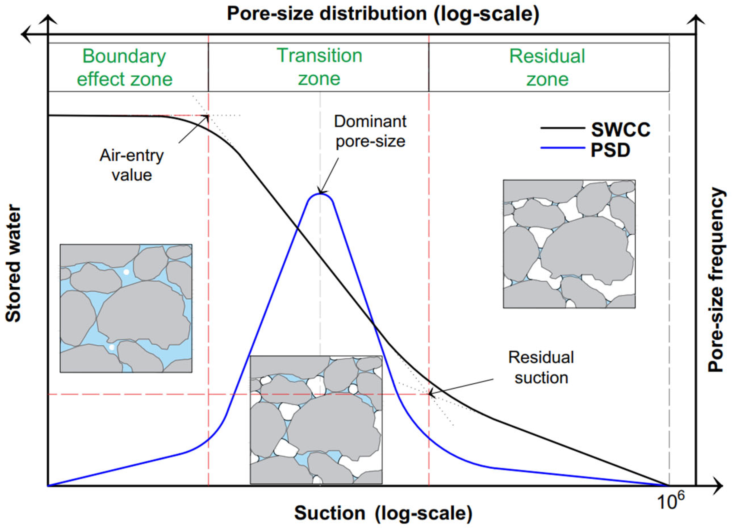
2.1. Basic Methodology for Modeling SWCC Based on the Matric Suction Variation

2.1.1. Basic Framework

In this section, the variation in soil suction due to several influential factors that include temperature, initial water content, initial stress state, and salt concentration is considered via the capillary law (i.e., Equation (2)). The variation in matric suction caused by various influential factors can be written as below.

$$d\psi =d\left(\frac{2T_s\mathrm{c}\mathrm{o}\mathrm{s}\theta }{r}\right)=\frac{\partial \psi }{\partial T}dT+\frac{\partial \psi }{\partial P_{comp}}d{P}_{comp}+\frac{\partial \psi }{\partial w_i}d{w}_i+\frac{\partial \psi }{\partial C}dC=\sum \frac{\partial \psi }{\partial {\varphi }_i}d{\varphi }_i$$

(6)

where T, P_comp, w_i, and c are temperature, initial compaction pressure, initial water content, and salt concentration, respectively, and φ_i refers to an influential factor.

Equation (7) can be obtained by expanding Equation (6), considering the variation in surface tension, contact angle, and pore radius caused by various factors (e.g., temperature, salt concentration [17,18,19,20,21,22]).

$$\begin{gathered} d\psi =\frac{2\mathrm{c}\mathrm{o}\mathrm{s}\theta }{r}\left(\frac{\partial T_s}{\partial T}dT+\frac{\partial T_s}{\partial P_{comp}}d{P}_{comp}+\frac{\partial T_s}{\partial w_i}d{w}_i+\frac{\partial T_s}{\partial C}dC\right)+\frac{2T_s}{r}\left[\frac{\partial \left(\mathrm{c}\mathrm{o}\mathrm{s}\theta \right)}{\partial T}dT+\frac{\partial \left(\mathrm{c}\mathrm{o}\mathrm{s}\theta \right)}{\partial P_{comp}}d{P}_{comp}+\frac{\partial \left(\mathrm{c}\mathrm{o}\mathrm{s}\theta \right)}{\partial w_i}d{w}_i+ \\ \frac{\partial \left(\mathrm{c}\mathrm{o}\mathrm{s}\theta \right)}{\partial C}dC\right]+\left(2T_s\mathrm{c}\mathrm{o}\mathrm{s}\theta \right)\left[\frac{\partial \left(\frac{1}{r}\right)}{\partial T}dT+\frac{\partial \left(\frac{1}{r}\right)}{\partial P_{comp}}d{P}_{comp}+\frac{\partial \left(\frac{1}{r}\right)}{\partial w_i}d{w}_i+\frac{\partial \left(\frac{1}{r}\right)}{\partial C}dC\right] \end{gathered}$$

(7)

Equation (7) suggests that temperature affects surface tension, contact angle, and the pore radius. This is a complex model considering the coupled influence of all the discussed parameters. In this study, the variations in surface tension and contact angle are analyzed together by simplifying Equation (7) into Equation (8), as given below.

$$\begin{gathered} d\psi =d\left(\frac{2T_s\mathrm{c}\mathrm{o}\mathrm{s}\theta }{r}\right)=\frac{1}{r}\left[\frac{\partial \left(2T_s\mathrm{c}\mathrm{o}\mathrm{s}\theta \right)}{\partial T}dT+\frac{\partial \left(2T_s\mathrm{c}\mathrm{o}\mathrm{s}\theta \right)}{\partial P_{comp}}d{P}_{comp}+\frac{\partial \left(2T_s\mathrm{c}\mathrm{o}\mathrm{s}\theta \right)}{\partial w_i}d{w}_i+\frac{\partial \left(2T_s\mathrm{c}\mathrm{o}\mathrm{s}\theta \right)}{\partial c}dc\right] \\ +\left(2T_s\mathrm{c}\mathrm{o}\mathrm{s}\theta \right)\left[\frac{\partial \left(\frac{1}{r}\right)}{\partial T}dT+\frac{\partial \left(\frac{1}{r}\right)}{\partial P_{comp}}d{P}_{comp}+\frac{\partial \left(\frac{1}{r}\right)}{\partial w_i}d{w}_i+\frac{\partial \left(\frac{1}{r}\right)}{\partial c}dc\right] \\ =\sum \left[\frac{\partial \left(2T_s\mathrm{c}\mathrm{o}\mathrm{s}\theta \right)}{\partial {\varphi }_i}d{\varphi }_i+\frac{\left(2T_s\mathrm{c}\mathrm{o}\mathrm{s}\theta \right)\partial \left(\frac{1}{r}\right)}{\partial {\varphi }_i}d{\varphi }_i\right] \end{gathered}$$

(8)

Equation (8) represents effects related to matric suction in two parts. The first part of the equation relates to the variation in air–water interfacial free energy (e.g., T_s cosθ), while the second part considers changes that arise in the pore radius. However, not all factors contribute equally to the variation in matric suction. For example, both initial compaction pressure and initial water content in a fine-grained soil may exert minor effects on surface tension and contact angle in comparison with their effects on pore radius.

In this study, temperature and salt concentration are also considered to play a role in the variation in air–water interface energy (e.g., surface tension and contact angle). To achieve this, Equation (8) is further simplified into Equation (9).

$$d\psi =d\left(\frac{2T_s\mathrm{c}\mathrm{o}\mathrm{s}\theta }{r}\right)=\frac{1}{r}\left(\frac{\partial \left(2T_s\mathrm{c}\mathrm{o}\mathrm{s}\theta \right)}{\partial T}dT+\frac{\partial \left(2T_s\mathrm{c}\mathrm{o}\mathrm{s}\theta \right)}{\partial c}dc\right)+\left(2T_s\mathrm{c}\mathrm{o}\mathrm{s}\theta \right)\left[\frac{\partial \left(\frac{1}{r}\right)}{\partial P_{comp}}d{P}_{comp}+\frac{\partial \left(\frac{1}{r}\right)}{\partial w_i}d{w}_i\right]$$

(9)

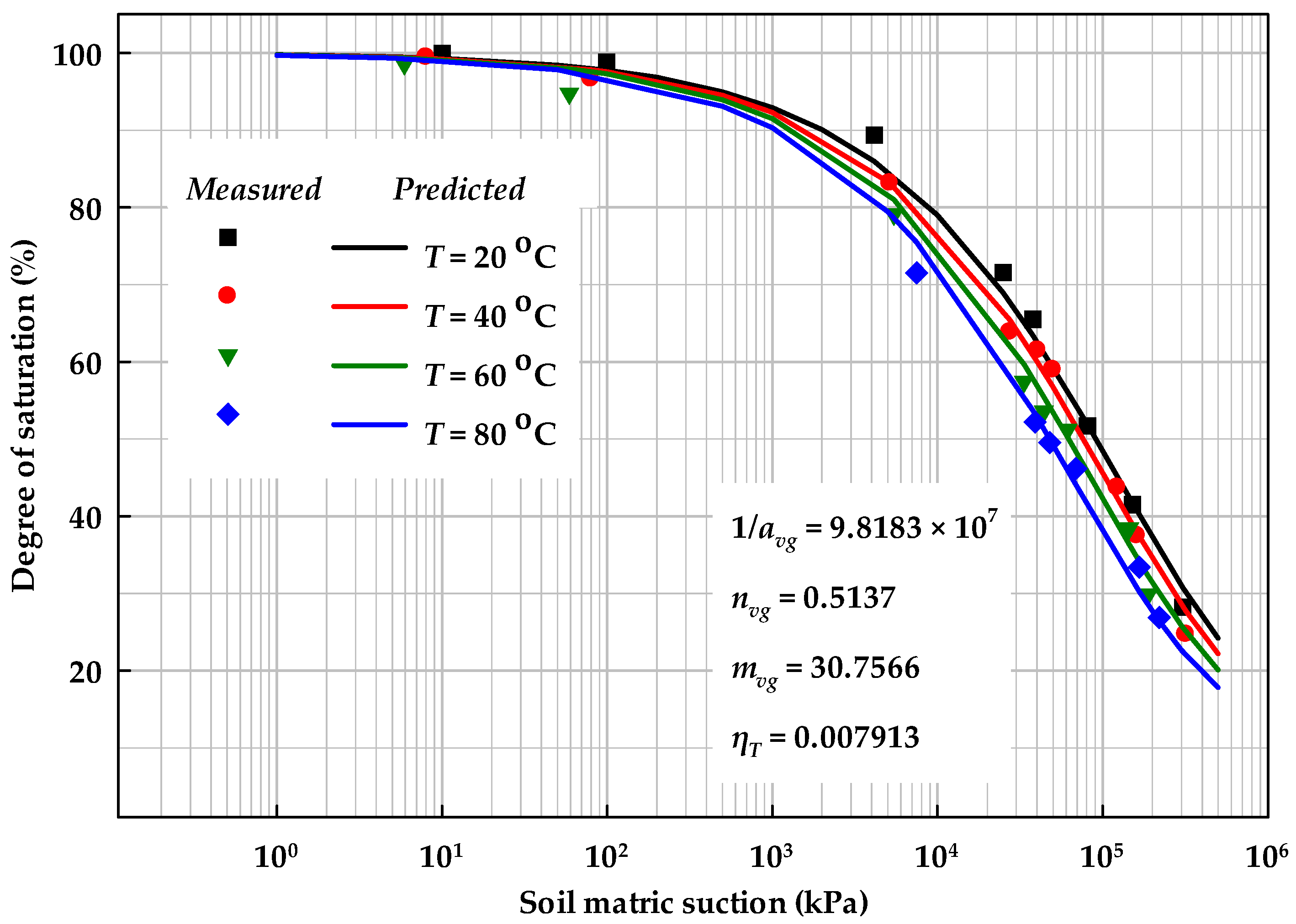
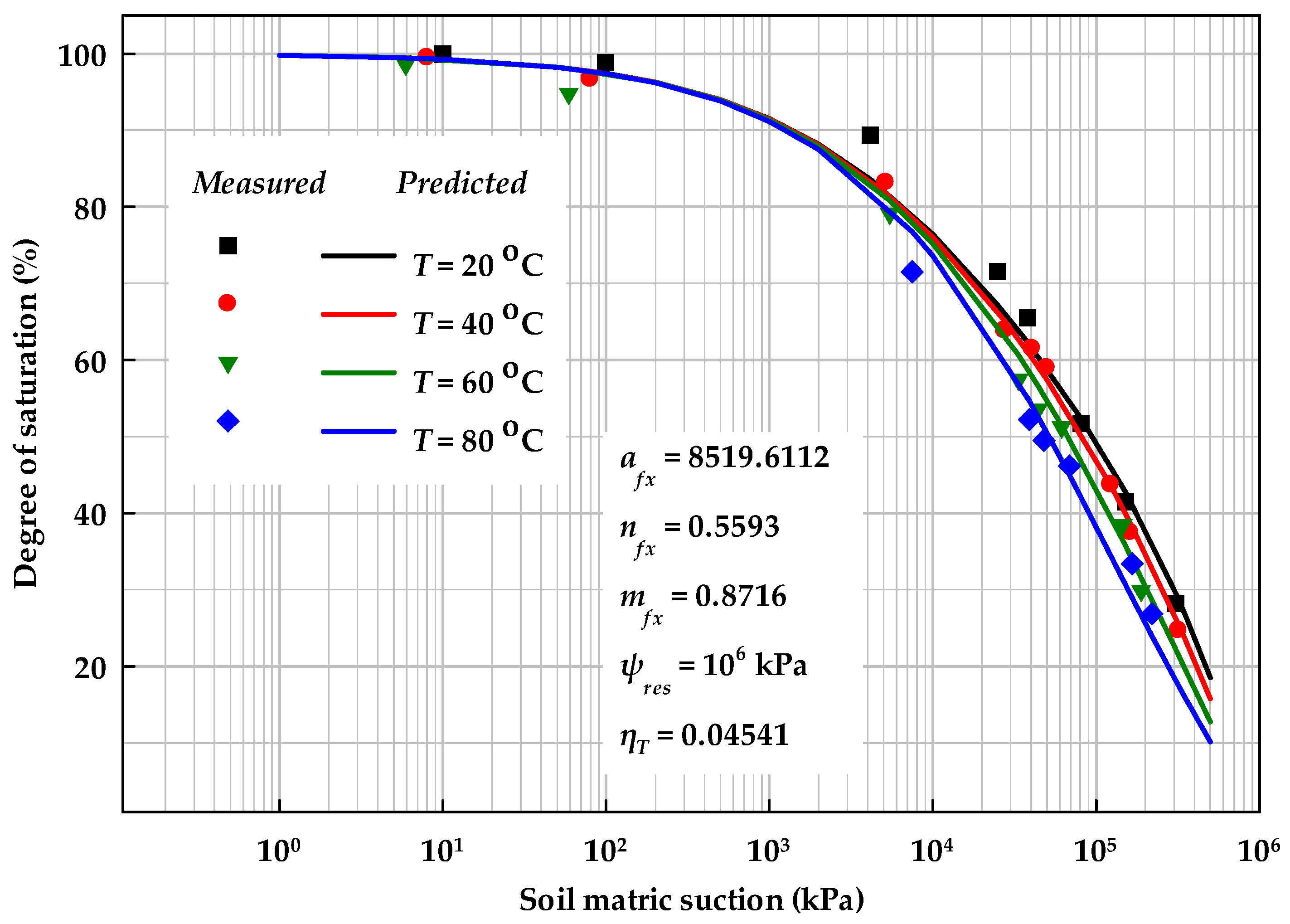
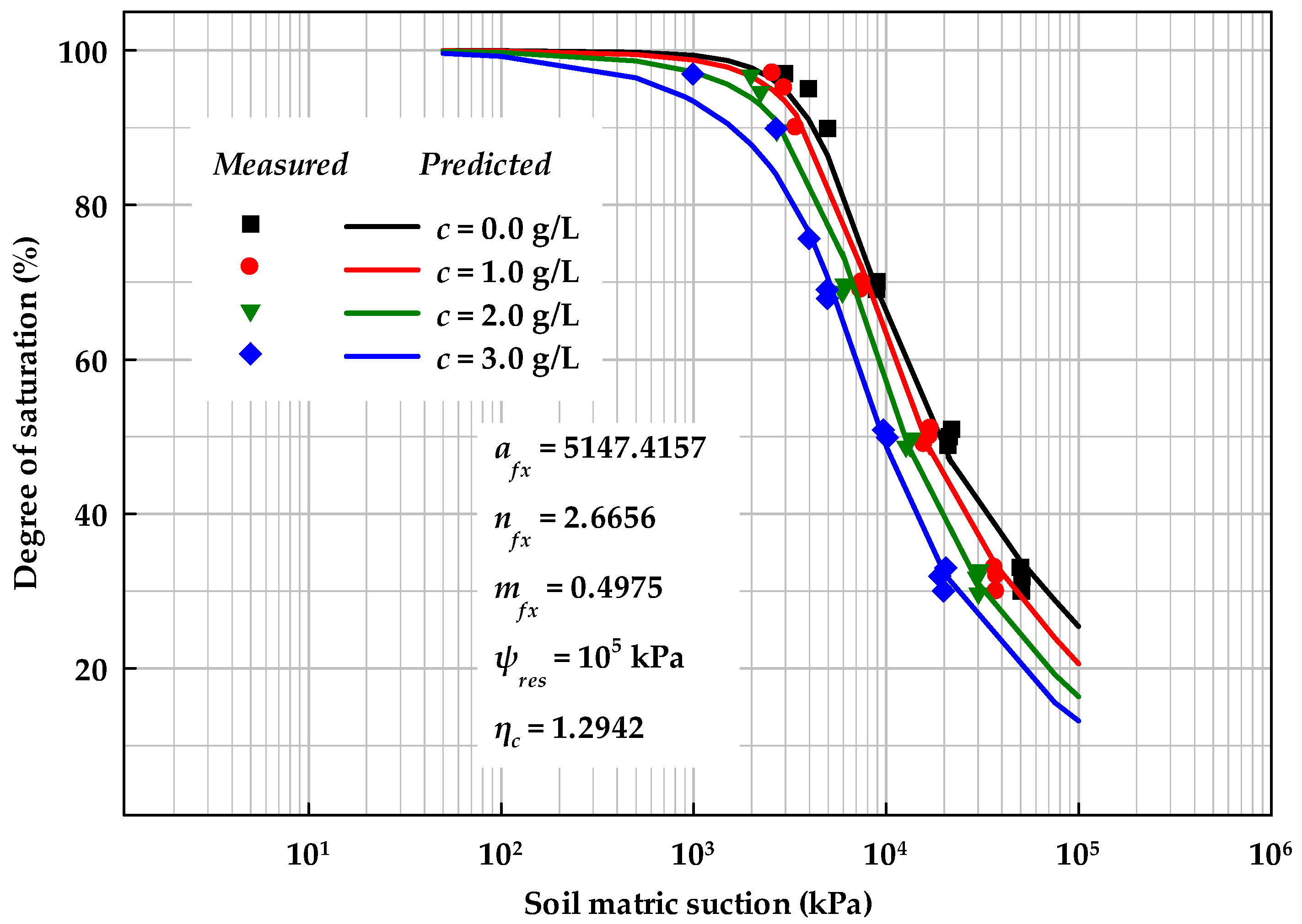
2.1.2. Temperature and Salt Solution Effects on Matric Suction

Experimental results published in the literature highlight a rough linear downward trend due to the influence of temperature and soluble salt concentration effects on air–water interface energy. Equations (10) and (11) are suggested to describe this trend, respectively, for temperature and salt solution (concentration).

$$\frac{\partial \left(2T_s\mathrm{c}\mathrm{o}\mathrm{s}\theta \right)}{\partial T}dT=-{\left(2T_s\mathrm{c}\mathrm{o}\mathrm{s}\theta \right)}_0{\eta }_{T}dT=-{\left(2T_s\mathrm{c}\mathrm{o}\mathrm{s}\theta \right)}_0{\eta }_T\left(T-T_0\right)$$

(10)

$$\frac{\partial \left(2T_s\mathrm{c}\mathrm{o}\mathrm{s}\theta \right)}{\partial c}dc=-{\left(2T_s\mathrm{c}\mathrm{o}\mathrm{s}\theta \right)}_0{\eta }_{c}dc=-{\left(2T_s\mathrm{c}\mathrm{o}\mathrm{s}\theta \right)}_0{\eta }_c\left(c-c_0\right)$$

(11)

where (2T_scosθ)₀ refers to the constant value in the original state (e.g., the value at T₀ and c₀).

Based on Equations (9)–(11), the following Equation (12) can be obtained.

$$\frac{{\psi }^{\prime }}{\psi }=\frac{\psi +\mathsf{\Delta }\psi }{\psi }\cong \frac{\psi +\mathrm{d}\psi }{\psi }=1-{\eta }_T\left(T-T_0\right)-{\eta }_c\left(c-c_0\right)$$

(12a)

$$\psi =\frac{{\psi }^{\prime }}{\left[1-{\eta }_T\left(T-T_0\right)-{\eta }_c\left(c-c_0\right)\right]}$$

(12b)

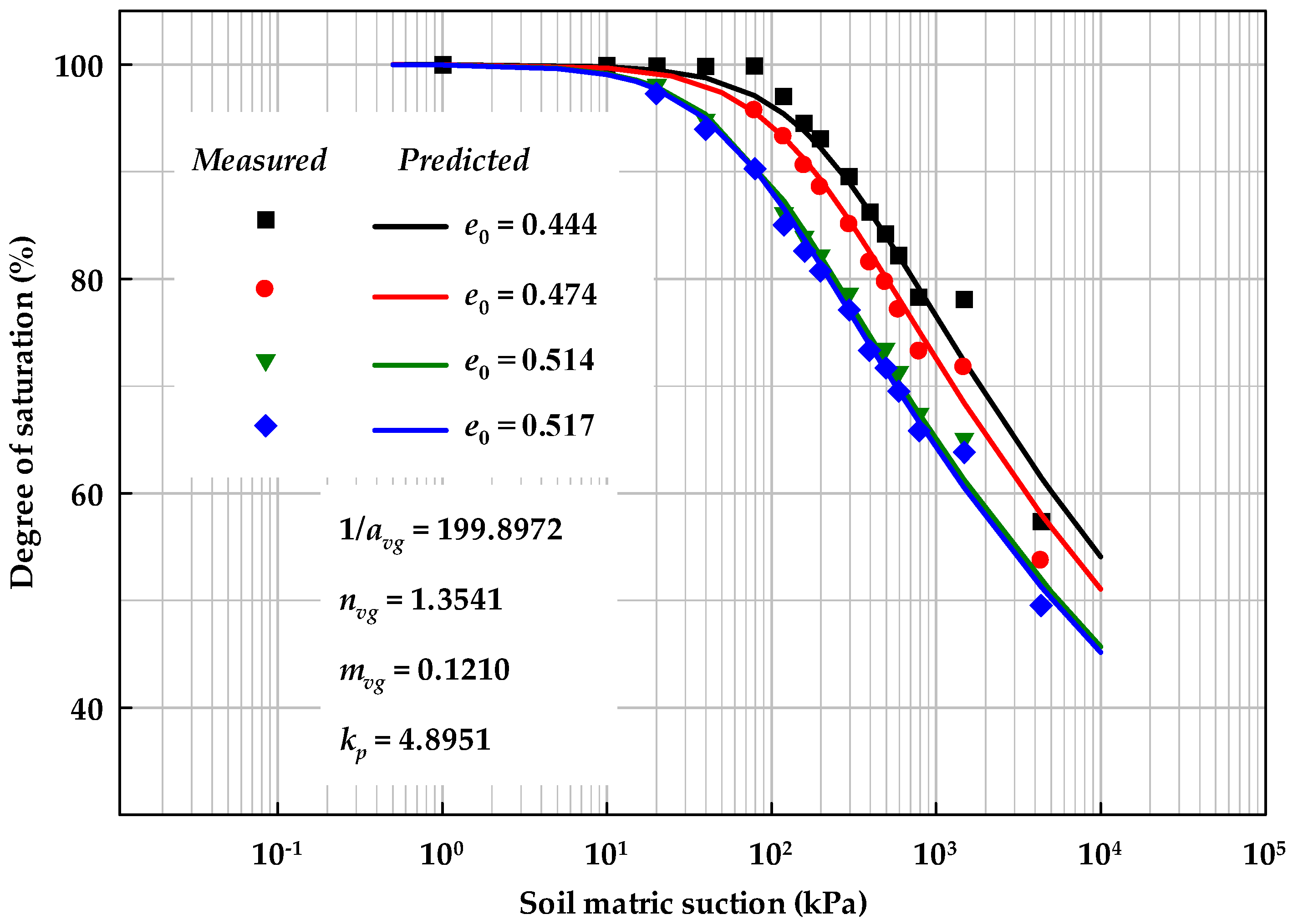
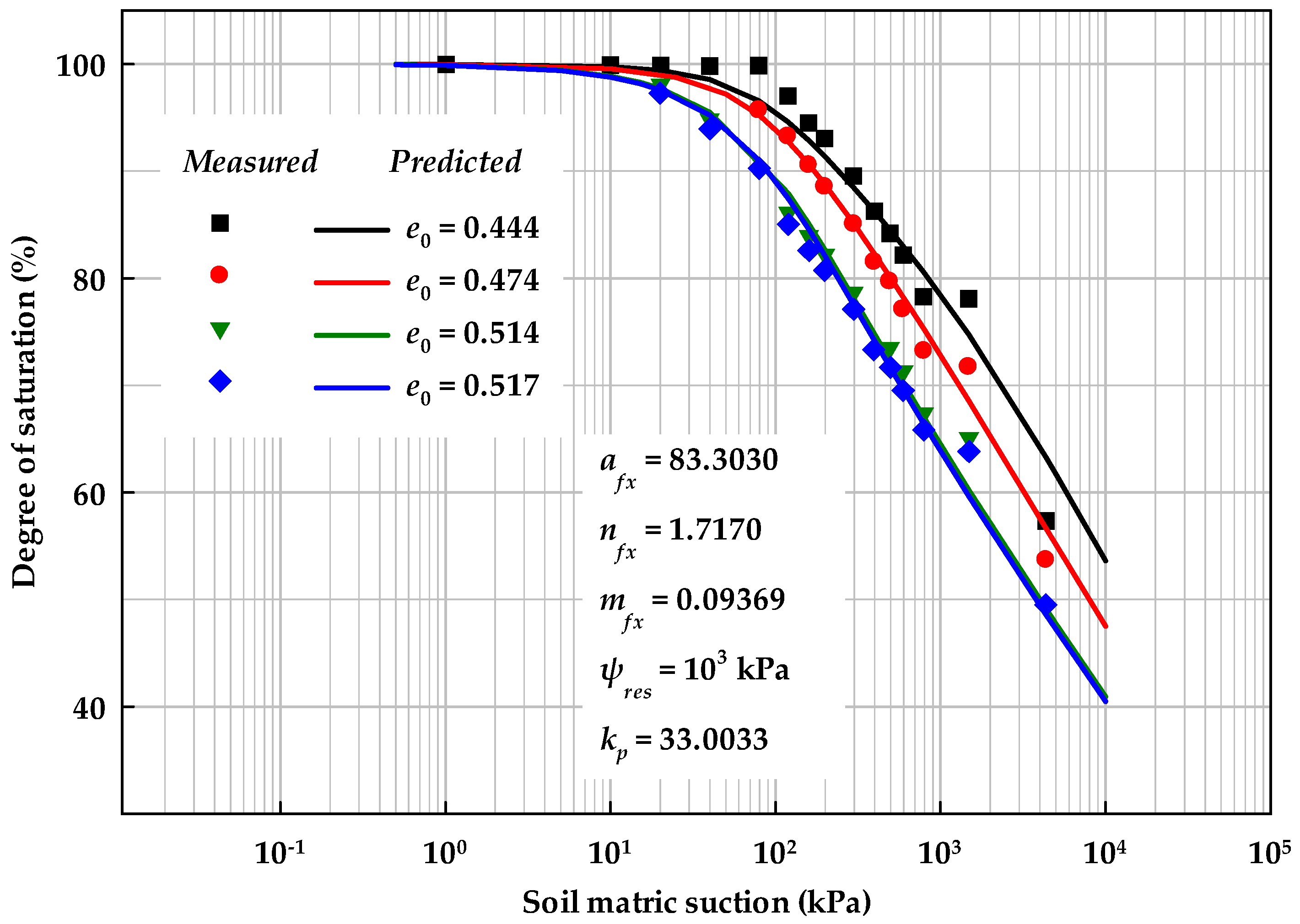
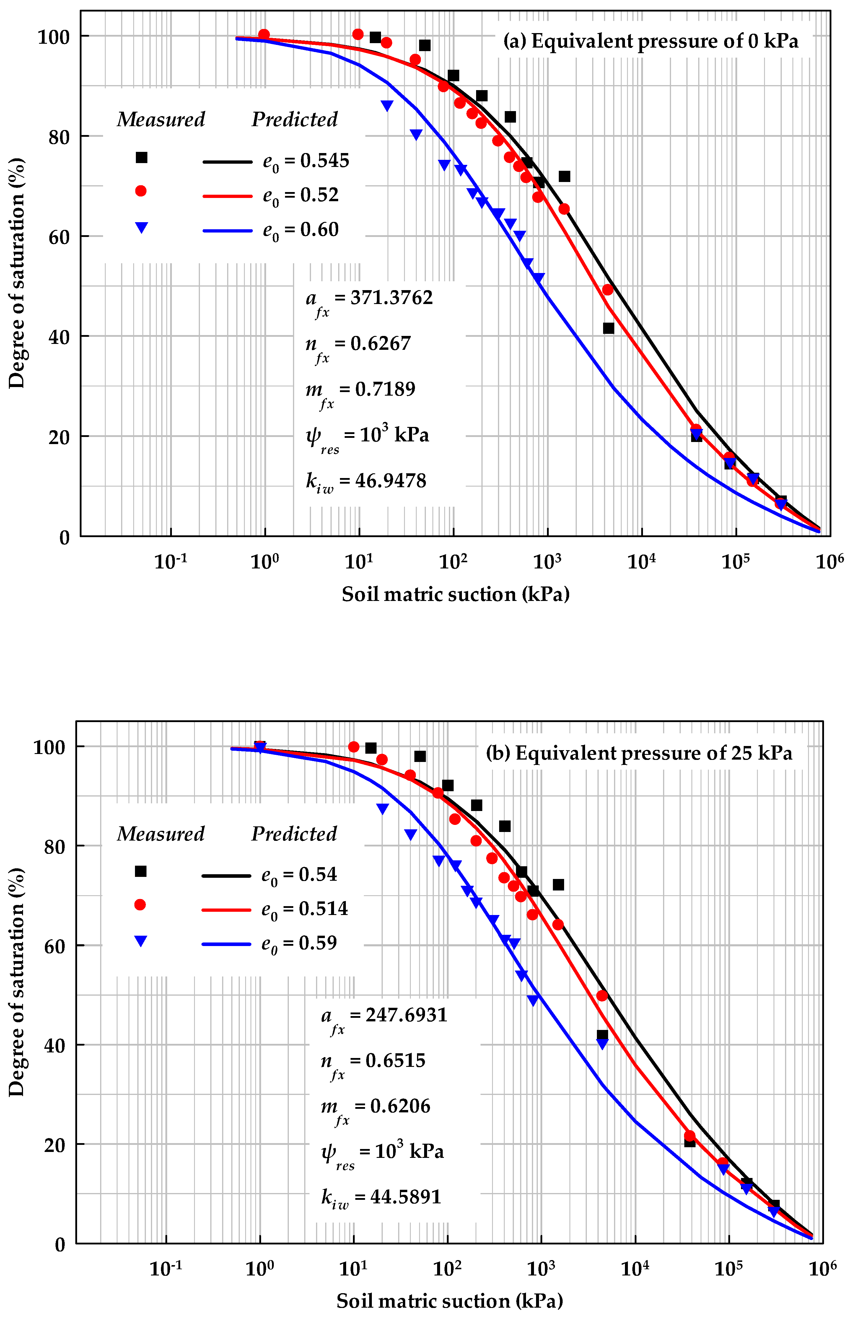
2.1.3. Initial Stress and Water Content Effects on Matric Suction

The second part on the right side of Equation (9) is useful for evaluating the influence of the initial stress effect.

$$\frac{\partial \left(\frac{1}{r}\right)}{\partial P_{comp}}d{P}_{comp}=-\frac{1}{r^2}\frac{\partial \left(r\right)}{\partial P_{comp}}d{P}_{comp}=\frac{1}{r}\left(-\frac{1}{r}\frac{\partial r}{\partial P_{comp}}d{P}_{comp}\right)$$

(13)

The right side of Equation (13) highlights the deformation of soil pores under compression. Equation (13) can model the variation in pore radius under initial compact pressure. However, a direct mathematical relationship between pore radius and compaction pressure is not established. In this regard, two equations—(14) and (15)—might be helpful. Equation (14) builds relationships between volumetric strain and one-dimensional deformation, while Equation (15) proposes a rather simplified link between volumetric strain and compression.

$${\epsilon }_v=-\frac{∆e}{1+e}=-\frac{∆V_{void}}{V}\cong -\left(\frac{∆l_x}{l_x}+\frac{∆l_y}{l_y}+\frac{∆l_z}{l_z}\right)=-3\frac{∆r}{r}$$

(14)

$$d{\epsilon }_v=k_c\frac{d{P}_{comp}}{P_{comp}}$$

(15)

where ε_v is volumetric strain (contraction is positive), e is the void ratio, V_void is the volume of soil void, l_x, l_y, and l_z refer to lengths in the x, y, and z axes, respectively, and k_c is a model parameter.

Equation (16) can be developed based on Equations (14) and (15).

$$\frac{\partial \left(\frac{1}{r}\right)}{\partial P_{comp}}d{P}_{comp}=\frac{1}{r}\left(-\frac{1}{r}\frac{\partial r}{\partial P_{comp}}d{P}_{comp}\right)=\frac{1}{r}\left(\frac{1}{3}\frac{d{\epsilon }_v}{\partial P_{comp}}d{P}_{comp}\right)=\frac{1}{r}\left(\frac{k_p}{P_{comp}}d{P}_{comp}\right)$$

(16)

where k_p is a model parameter.

Similar to Equation (12a), the following Equation (17) can be obtained.

$$\frac{{\psi }^{\prime }}{\psi }=\frac{\psi +\mathsf{\Delta }\psi }{\psi }\cong \frac{\psi +\mathrm{d}\psi }{\psi }=\frac{\psi +\left(2T_s\mathrm{c}\mathrm{o}\mathrm{s}\theta \right)\left(\frac{\partial \left(\frac{1}{r}\right)}{\partial P_{comp}}d{P}_{comp}\right)}{\psi }=\frac{1+k_p\frac{∆P_{comp}}{P_{comp}}}{1}=1+k_p\left(1-P_0/P_{comp}\right)$$

(17)

Equation (18) can be used to model the initial water content effect at wetting optimum.

$$\frac{\partial \left(\frac{1}{r}\right)}{\partial w_i}d{w}_i=-\frac{1}{r^2}\frac{\partial r}{\partial w_i}d{w}_i=\frac{1}{r}\left(-\frac{1}{r}\frac{\partial r}{\partial w_i}d{w}_i\right)=\frac{1}{r}\left(\frac{1}{3}\frac{d{\epsilon }_v}{\partial w_i}d{w}_i\right)$$

(18)

The relationships between initial water content and soil matric suction can be evaluated from the BC model (i.e., Equation (19a)). An equation similar to Equation (15) can be found in Equation (19b) for evaluating the effect of volumetric strain on matric suction. Equation (19b) is a simplified model for understanding volume deformation under matric suction.

$$\frac{w_i}{w_0}\cong {\left(\frac{{\psi }_0}{{\psi }_i}\right)}^{{\lambda }_{bc}}$$

(19a)

$$d{\epsilon }_v=k_{\psi }\frac{d{\psi }_i}{{\psi }_i}$$

(19b)

Based on Equations (19), relationships between initial water content and volumetric deformation can be summarized as Equation (20).

$$d{w}_i=-{\lambda }_{bc}{w}_0{\left(\frac{{\psi }_0}{{\psi }_i}\right)}^{{\lambda }_{bc}}\frac{d{\psi }_i}{{\psi }_i}=-\frac{{\lambda }_{bc}}{k_{\psi }}{w}_0{\left(\frac{{\psi }_0}{{\psi }_i}\right)}^{{\lambda }_{bc}}\left(k_{\psi }\frac{d{\psi }_i}{{\psi }_i}\right)=-\frac{{\lambda }_{bc}}{k_{\psi }}{w}_0{\left(\frac{{\psi }_0}{{\psi }_i}\right)}^{{\lambda }_{bc}}d{\epsilon }_v=-\frac{{\lambda }_{bc}}{k_{\psi }}{w}_{i}d{\epsilon }_v$$

(20)

Based on Equation (20), Equation (18) can be modified and summarized as Equation (21).

$$\frac{\partial \left(\frac{1}{r}\right)}{\partial w_i}d{w}_i=\frac{1}{r}\left(\frac{1}{3}\frac{d{\epsilon }_v}{\partial w_i}d{w}_i\right)=\frac{1}{r}\left(-\frac{1}{3}\frac{k_{\psi }}{{\lambda }_{bc}}\frac{d{w}_i}{w_i}\right)=\frac{1}{r}\left(-\frac{k_{iw}}{w_i}d{w}_i\right)$$

(21)

Equation (21) can be represented in a form shown in Equation (22).

$$\frac{{\psi }^{\prime }}{\psi }=\frac{\psi +\mathsf{\Delta }\psi }{\psi }\cong \frac{\psi +\mathrm{d}\psi }{\psi }=\frac{\psi +\left(2T_s\mathrm{c}\mathrm{o}\mathrm{s}\theta \right)\left(\frac{\partial \left(\frac{1}{r}\right)}{\partial w_i}d{w}_i\right)}{\psi }=\frac{1-\frac{k_{iw}}{w_i}∆w_i}{1}=1-k_{iw}\left(1-w_0/w_i\right)$$

(22)

where k_iw is a model parameter, and w₀ is the initial water content at reference state.

Equation (22) is built for modeling the SWCCs of fine-grained soils with initial water contents on the wetting side of the optimum water content. For water contents at dry side of optimum, the initial void ratio decreases (or initial dry density increases) as the initial water content rises. To express the initial water content effect at dry side of optimum, Equation (23) is suggested.

$$\frac{{\psi }^{\prime }}{\psi }=\frac{\psi +\mathsf{\Delta }\psi }{\psi }=1+k_{iw}\left(1-w_0/w_i\right)$$

(23)

Equation (24) can be obtained based on Equations (9), (12), (17), (22), and (23). Equation (24a) considers the influence of initial water content in compacted fine-grained soils on wet of optimum conditions. Equation (24b) can be used for fine-grained soils compacted in conditions that are dry of optimum. The variation of soil matric suction can be numerically evaluated by substituting Equation (24) directly into Equation (4b).

$$\psi =\frac{{\psi }^{\prime }}{\left[1-{\eta }_T\left(T-T_0\right)-{\eta }_c\left(c-c_0\right)+k_p\left(1-P_0/P_{comp}\right)-k_{iw}\left(1-w_0/w_i\right)\right]}$$

(24a)

$$\psi =\frac{{\psi }^{\prime }}{\left[1-{\eta }_T\left(T-T_0\right)-{\eta }_c\left(c-c_0\right)+k_p\left(1-P_0/P_{comp}\right)+k_{iw}\left(1-w_0/w_i\right)\right]}$$

(24b)

In some cases, the initial void ratio is used instead of the initial stress state and the initial water content. For the initial stress state and the initial water content at dry optimum of condition, the initial void ratio decreases with the rise of equivalent compaction pressure and the initial water content (e.g., Equation (25b)). Due to the change in soil structure that arises in fine-grained soils because of the higher initial water content in the wet of optimum water content, there will be a rise in initial void ratio that can be attributed to the variation in smaller pores [37]. Equation (25a) can be used for representing such a scenario. Equation (25b) can be used for soils compacted at dry of optimum conditions.

$$\psi =\frac{{\psi }^{\prime }}{\left[1-{\eta }_T\left(T-T_0\right)-{\eta }_c\left(c-c_0\right)-k_p\left(1-e_0/e_{comp}\right)+k_{iw}\left(1-e_0/e_i\right)\right]}$$

(25a)

$$\psi =\frac{{\psi }^{\prime }}{\left[1-{\eta }_T\left(T-T_0\right)-{\eta }_c\left(c-c_0\right)-k_p\left(1-e_0/e_{comp}\right)-k_{iw}\left(1-e_0/e_i\right)\right]}$$

(25b)

where e₀ is the initial void ratio at reference state, and e_comp and e_i refer to the initial void ratios at corresponding initial stress state and initial water content, respectively.

The effects of various factors that include temperature, salt solution, initial stress state, and initial water content on SWCCs are highlighted in Figure 3, Figure 4, Figure 5 and Figure 6, respectively, which were numerically modeled using Equation (25) by substituting that into Equation (4b).

2.1.4. Coupling Effects on Soil Matric Suction

Based on Equation (25), these factors affect each other in a coupled manner. Another feasible approach can be evaluated using Equation (26) by neglecting high-order terms.

$$\begin{gathered} d\psi =d\left(\frac{2T_s\mathrm{c}\mathrm{o}\mathrm{s}\theta }{r}\right)=\frac{\partial \psi }{\partial {\varphi }_i}\left({\varphi }_i-{\varphi }_0\right)+\frac{\partial \psi }{\partial {\varphi }_j}\left({\varphi }_j-{\varphi }_0\right)+\frac{{\partial }^2\psi }{2\partial {\varphi }_i\partial {\varphi }_i}{\left({\varphi }_i-{\varphi }_0\right)}^2+\frac{{\partial }^2\psi }{2\partial {\varphi }_j\partial {\varphi }_j}{\left({\varphi }_j-{\varphi }_0\right)}^2 \\ +\frac{{\partial }^2\psi }{\partial {\varphi }_i\partial {\varphi }_j}\left({\varphi }_i-{\varphi }_0\right)\left({\varphi }_j-{\varphi }_0\right)\cong \frac{\partial \psi }{\partial {\varphi }_i}\left({\varphi }_i-{\varphi }_0\right)+\frac{\partial \psi }{\partial {\varphi }_j}\left({\varphi }_j-{\varphi }_0\right)+\frac{{\partial }^2\psi }{\partial {\varphi }_i\partial {\varphi }_j}\left({\varphi }_i-{\varphi }_0\right)\left({\varphi }_j-{\varphi }_0\right) \end{gathered}$$

(26)

where ϕ_i and ϕ_j represent two distinct influential factors.

For the pore air–water interfacial energy part (e.g., 2T_s cosθ), the coefficient on the right side of Equation (26) can be treated as a constant for simplicity. The high-order term for the variation of pore radius can be modeled using the relationship below.

$$\frac{{\partial }^2\left(\frac{2T_s\mathrm{c}\mathrm{o}\mathrm{s}\theta }{r}\right)}{\partial {\varphi }_i\partial {\varphi }_j}d{\varphi }_{i}d{\varphi }_j=2T_s\mathrm{c}\mathrm{o}\mathrm{s}\theta \frac{2}{r^3}\frac{{\partial }^{2}r}{\partial {\varphi }_i\partial {\varphi }_j}d{\varphi }_{i}d{\varphi }_j=\frac{2T_s\mathrm{c}\mathrm{o}\mathrm{s}\theta }{r}\frac{2}{r^2}\frac{{\partial }^{2}r}{\partial {\varphi }_i\partial {\varphi }_j}d{\varphi }_{i}d{\varphi }_j=\frac{2T_s\mathrm{c}\mathrm{o}\mathrm{s}\theta }{r}\frac{2}{r^2}\frac{{\partial }^{2}r}{\partial {\varphi }_i\partial {\varphi }_j}d{\varphi }_{i}d{\varphi }_j$$

(27)

Various SWCC models can be built considering the mutual effects of influential factors using Equation (27). However, due to limited experimental studies in the literature, the framework related to this part of the approach is proposed but not validated.

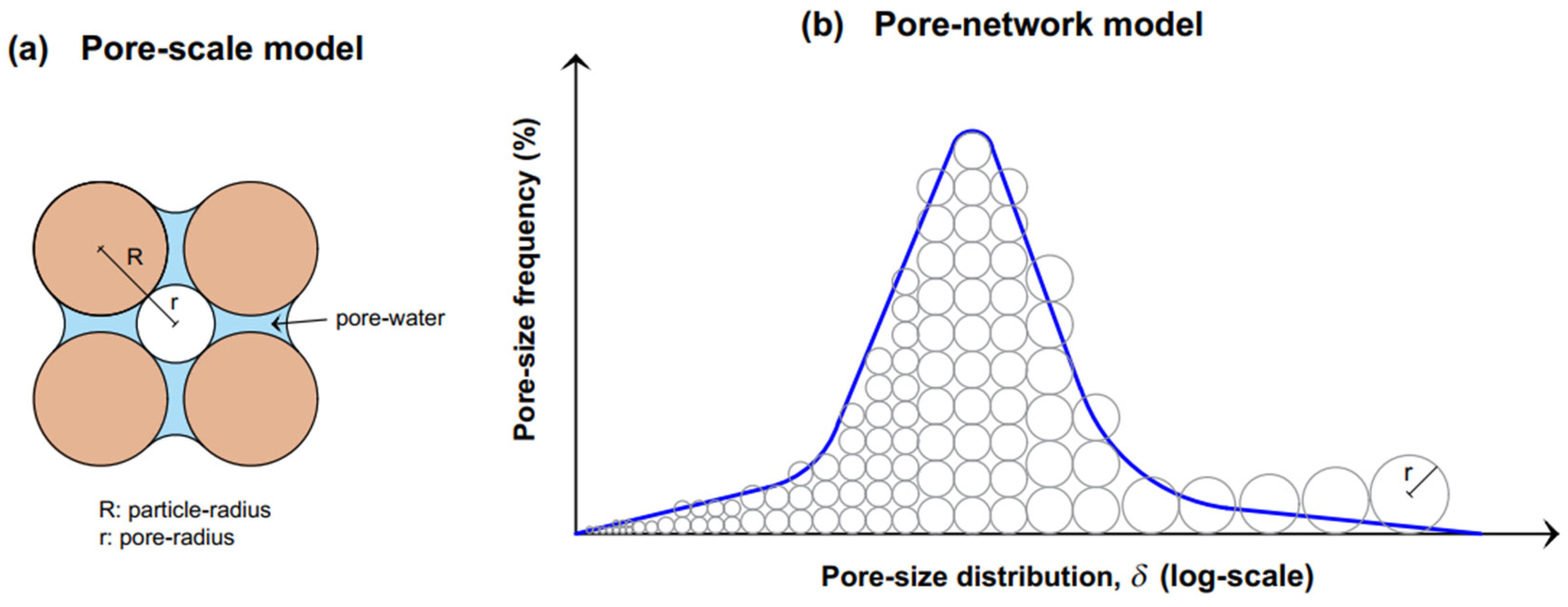
2.2. Basic Methodology for Representing Pore Size Distribution Variation Using the SWCC Correction Function

In Section 2.1, the variation of soil matric suction due to various influential factors was investigated. As PoSD also has a significant influence on SWCC behavior, this section focuses on the variation in the PoSD induced by factors such as initial water content and initial stress state.

The FX model without a correction function (i.e., Equations (2) and (4)) can also be written in a differential form, as summarized in Equation (28a).

$$\theta \left(\psi \right)={\int }_{\psi }^{{\psi }_{max}}f\left(\psi \right)d\psi ={\int }_{\psi }^{{\psi }_{max}}\frac{m_{fx}{n}_{fx}{(\psi /a_{fx})}^{n_{fx}-1}}{a_{fx}\left[\mathrm{e}\mathrm{x}\mathrm{p}\left(1\right)+{\left(\psi /a_{fx}\right)}^{n_{fx}}\right]{\left[\mathrm{l}\mathrm{n}\left(\mathrm{e}\mathrm{x}\mathrm{p}\left(1\right)+{\left(\psi /a_{fx}\right)}^{n_{fx}}\right)\right]}^{m_{fx}+1}}d\psi$$

(28a)

$$\begin{gathered} \theta \left(\psi \right)={\int }_{\psi }^{{\psi }_{max}}h\left(\psi \right)f\left(\psi \right)d\psi = \\ {\int }_{\psi }^{{\psi }_{max}}h\left(\psi \right)\frac{m_{fx}{n}_{fx}{(\psi /a_{fx})}^{n_{fx}-1}}{a_{fx}\left[\mathrm{e}\mathrm{x}\mathrm{p}\left(1\right)+{\left(\psi /a_{fx}\right)}^{n_{fx}}\right]{\left[\mathrm{l}\mathrm{n}\left(\mathrm{e}\mathrm{x}\mathrm{p}\left(1\right)+{\left(\psi /a_{fx}\right)}^{n_{fx}}\right)\right]}^{m_{fx}+1}}d\psi \end{gathered}$$

(28b)

$$\left\{\begin{array}{l}h\left(0\right)=0\\ {\int }_0^{{\psi }_{max}}h\left(\psi \right)d\psi =1\end{array}\right.$$

(28c)

To represent the variation in PoSD, one function h(ψ) can be added into PoSD, as shown in Equation (28b). Function h(ψ) should satisfy the boundary conditions (i.e., Equation (28c)), which equals zero at saturation, and its integral is one over the entire soil suction. To simplify the integral of the expression in Equation (28b), the following Equation (29) is suggested.

$$\begin{gathered} \theta \left(\psi \right)={\int }_{\psi }^{{\psi }_{max}}h\left(\psi \right)d\psi {\int }_{\psi }^{{\psi }_{max}}f\left(\psi \right)d\psi = \\ {\int }_{\psi }^{{\psi }_{max}}h\left(\psi \right)d\psi {\int }_{\psi }^{{\psi }_{max}}\frac{m_{fx}{n}_{fx}{(\psi /a_{fx})}^{n_{fx}-1}}{a_{fx}\left[\mathrm{e}\mathrm{x}\mathrm{p}\left(1\right)+{\left(\psi /a_{fx}\right)}^{n_{fx}}\right]{\left[\mathrm{l}\mathrm{n}\left(\mathrm{e}\mathrm{x}\mathrm{p}\left(1\right)+{\left(\psi /a_{fx}\right)}^{n_{fx}}\right)\right]}^{m_{fx}+1}}d\psi \end{gathered}$$

(29)

Using Equation (29), the method to find function h(ψ) can be simplified to model the soil volumetric deformation observed over the soil suction increase (see Figure 7). As soil volume change will clearly result in pore size change, a function to represent soil deformation under variation of matric suction is reasonable.

The following two features should be highlighted: first, the soil deformation in unsaturated soils is predominant within the boundary effect and transition zone, which is typically within several hundred kPa of matric suction [38], as shown in Figure 7. However, some clayey soils may not desaturate as the air-entry value may not be reached within this suction range (i.e., soil is near saturation and correction function is near one). Second, soil pores with varied sizes will be drained at a certain matric suction, typically larger than the air-entry value (i.e., the soil is in an unsaturated state and the correction function plays a role over the entire range of matric suction).

To satisfy the above criteria, two assumptions must be highlighted. The first assumption is the terminal point of volume change under matric suction (e.g., point R_c in Figure 7b). After this point, there can still be some volume change in unsaturated soils. However, the associated volume change due to the influence of this suction is relatively small and hence can be neglected. The second assumption is that at 10⁶ kPa, soil will have (almost) zero water content. Both these assumptions are reasonable and are used in the rational explanation of the mechanics of unsaturated soils.

These assumptions or conditions can be introduced into one of the most suitable equations, which is the correction function in Equation (5b). The following Equation (30) is suggested to model THMC (e.g., temperature, salt solution, initial stress state, and initial water content) effects on SWCCs based on the correction function.

$$c\left(\psi \right)=\left[1-\frac{\mathrm{l}\mathrm{n}\left[1+\left(\psi /{\psi }_{res}\right)\right]}{\mathrm{l}\mathrm{n}\left[1+\left({10}^6/{\psi }_{res}\right)\right]}\right]$$

(30a)

$${\psi }_{res}={\psi }_{res0}\mathrm{e}\mathrm{x}\mathrm{p}\left(-{\eta }_T\left(T-T_0\right)-{\eta }_c\left(c-c_0\right)-k_p\left(e_{comp}-e_0\right)-k_{iw}\left(e_i-e_0\right)\right)$$

(30b)

$${\psi }_{res}={\psi }_{res0}\mathrm{e}\mathrm{x}\mathrm{p}\left(k_{iw}\left(e_i-e_0\right)\right), \mathrm{f}\mathrm{o}\mathrm{r} \mathrm{w}\mathrm{e}\mathrm{t}\mathrm{t}\mathrm{i}\mathrm{n}\mathrm{g} \mathrm{o}\mathrm{p}\mathrm{t}\mathrm{i}\mathrm{m}\mathrm{u}\mathrm{m}$$

(30c)

where exp () is the exponential function.

It should be noted that residual suction ψ_res in Equation (30a) is regarded as a model parameter to obtain the best model performance. Equation (30b) is a general equation for predicting SWCC under temperatures, salt solutions, initial stress states, and initial water contents at dry of optimum side. Equation (30c) is suggested for predicting SWCC for both the wet of optimum side from optimum and dry of optimum sides. More information related to this method is available in [37]. The model results for THMC (e.g., temperature, salt solution, initial stress state, and initial water content) effects are highlighted in Figure 8, Figure 9, Figure 10 and Figure 11, respectively.

The correction function Equation (30a) can also be used to predict the main wetting curve from the main drying curve. Based on previous studies from the literature, the following Equation (31) is suggested.

$$\frac{{\theta }_{lw}-{\theta }_{res}}{{\theta }_{sat}-{\theta }_{res}}=c\left(\psi \right)·\frac{1}{{\left\{\mathrm{l}\mathrm{n}\left[\mathrm{e}\mathrm{x}\mathrm{p}\left(1\right)+{\left(\psi /a_{fx}\right)}^{n_{fx}}\right]\right\}}^{m_{fx}}}$$

(31a)

$$c\left(\psi \right)=\left[1-\frac{\mathrm{l}\mathrm{n}\left[1+\left(\psi -P_b\right)/{\psi }_{res}\right]}{\mathrm{l}\mathrm{n}\left[1+\left(P_a-P_b\right)/{\psi }_{res}\right]}\right],0\le c\left(\psi \right)\le 1$$

(31b)

where P_a is a model parameter, and P_b is regarded as the merging point between the main wetting and drying curves (see Figure 12).

The residual water content in Equation (31a) is highlighted, and the correction function in Equation (31b) should always be between zero and one. The prediction results for the main wetting curve from the main drying curve are presented in Figure 12.

Based on Equations (5c), (29), and (31), the models for drying scanning curves can be written as follows in Equation (32).

$$\frac{\theta -{\theta }_r}{{\theta }_0-{\theta }_r}=c\left(\psi \right)·\left(1-\frac{{\int }_{\psi }^{{\psi }_0}f\left(\psi \right)d\psi }{{\int }_{{\psi }_r}^{{\psi }_0}f\left(\psi \right)d\psi }\right)$$

(32a)

$$c\left(\psi \right)=\left[1-\frac{\mathrm{l}\mathrm{n}\left[1+\left(\psi -{\psi }_0\right)/{\psi }_{res}\right]}{\mathrm{l}\mathrm{n}\left[1+\left(P_a-{\psi }_0\right)/{\psi }_{res}\right]}\right],0\le c\left(\psi \right)\le 1$$

(32b)

Similarly, for wetting scanning curves, the models can be written as follows in Equation (33) based on the FX model.

$$\frac{\theta -{\theta }_0}{{\theta }_s-{\theta }_0}=c\left(\psi \right)·\frac{{\int }_{{\psi }_0}^{\psi }f\left(\psi \right)d\psi }{{\int }_{{\psi }_0}^{0}f\left(\psi \right)d\psi }$$

(33a)

$$c\left(\psi \right)=\left[1-\frac{\mathrm{l}\mathrm{n}\left[1+\left(\psi -P_b\right)/{\psi }_{res}\right]}{\mathrm{l}\mathrm{n}\left[1+\left(P_a-P_b\right)/{\psi }_{res}\right]}\right],0\le c\left(\psi \right)\le 1$$

(33b)

where ψ₀ and θ₀ refer to the start points of scanning curves. θ_r and θ_s in Equations (32a) and (33a), respectively, refer to the volumetric water at the merging point (slightly different from the original values).

Based on Equations (32) and (33) for drying and wetting scanning curves, respectively, the model performance is highlighted in Figure 13. θ_r and θ_s in Equations (32) and (33) equal 10.18% and 30.16%, respectively. In the two equations, P_a is regarded as a fitting parameter, while parameter P_b is regarded as the soil suction value at the merging point (i.e., 1.1 kPa in this case).

By repeatedly using Equations (5c), (32), and (33), the cyclic wetting and drying behaviors of SWCCs can be readily modeled. The modeling results are highlighted in Figure 14, while experimental results from the literature [39] are offered for comparison. One point should be noted: in Figure 14b, the value of parameter a_fx for the main wetting curve (i.e., parameter a_wet) differs from that for the main drying curve.

3. Model Results and Discussion

Figure 2 highlights the two methods applied to model SWCCs in this study. These two methods are prevailing and can function well to predict the variation in SWCCs under THMC (i.e., temperature, salt solution, initial stress state, and initial water content) effects, as highlighted in the figures. However, these are not the only methods for modeling SWCCs.

Figure 3 and Figure 8 highlight SWCC model prediction results when using these two distinct methods, shown in comparison with experimental data [22]. It should be noted that temperature affects pore sizes and air–water interfacial energy in combination, but in this study, these effects were separately modeled. Systematic research on temperature effects is, therefore, necessary.

Figure 4 and Figure 9 present SWCC prediction model results for salt solution effects, based on experiments presented in the literature [21]. Note that, in this study, only variation in matric suction was modeled, and the influence of osmotic suction was not considered. As shown by the van’t Hoff equation for osmotic pressure, osmotic suction should be treated as a constant under a certain solution concentration. However, due to electrical double layers around clayey particles, the ion concentration may not be constant in free water of unsaturated soils.

Figure 5 and Figure 10 present the initial stress state effects on SWCCs based on the experimental results in the literature [3]. Here, the initial void ratio is adopted instead of the initial compact pressure, as the void ratio is a smaller value and will increase the flexibility of the proposed models.

Figure 6 and Figure 11 further highlight the prediction results of the initial water content effects on SWCCs, as determined using experimental results from the literature [3]. In Figure 10 and Figure 11, the residual soil suction is regarded as a model parameter. Note that its value might not represent the exact amount of soil residual suction. The associated variation in PoSD is highlighted based on Equations (30), while the physical meanings of the parameter are omitted.

Figure 7 demonstrates the reason to treat the residual soil suction as a model parameter. Experimental data were gathered from [12]. As highlighted in the figure, a relatively smaller residual suction value can also be used to predict SWCC effectively. This perhaps owes to the flexibility of SWCC equations. Another reason, as discussed in the previous section, may be a feature of SWCC, whereby the correction function is highlighted in a high soil suction range (e.g., larger than 10⁵ kPa) while the residual value (10⁴ kPa in Figure 7b) might be more related to the turning point in the correction function before the soil suction limit (e.g., 10⁶ kPa). The gap between the roles of the correction function and the residual suction inside the correction function reserves space for modeling SWCCs flexibly.

The model results for predicting the main wetting curves from the main drying curves are highlighted in Figure 12. Experimental results were gathered from [23] and [10], respectively. Red dash lines (as well as red and blue circles) in Figure 12 are the experimental results. Our method was consistent with that in a previous study [37], though the role of the correction function was particularly highlighted in the present model (see Equation (31)). The prediction results obtained using the correction function, shown in Figure 8, Figure 9, Figure 10, Figure 11 and Figure 12, are based on the concept of pore size distribution (or the correction function in SWCC models). The success of predicting THMC (i.e., temperature, salt solution, initial stress state, and initial water content) effects and hysteretic effects on SWCCs (i.e., Equations (30) and (31)) reveals that the suggested unified model is promising for considering the variation of the correction function in SWCC equations.

Figure 13 and Figure 14 highlight the model results for hysteretic behaviors of SWCCs. Solid lines and dots are prediction and experimental results, respectively for Figure 3, Figure 4, Figure 5, Figure 6, Figure 7, Figure 8, Figure 9, Figure 10, Figure 11, Figure 12 and Figure 13 and Figure 14b. A distinct parameter a_fx value for the main wetting curve (i.e., parameter a_wet) was used to simplify calibration procedures. All the scanning curves in the figures were predicted using Equations (32) and (33), i.e., the correction function in the FX model.

4. Conclusions

In this article, two methods that address the variation in soil matric suction and pore size distribution (PoSD), respectively, have been highlighted for modeling THMC (e.g., temperature, salt solution, initial stress state, and initial water content) effects on SWCCs using well-known SWCC equations and correction functions, respectively.

The model results of both methods provide close comparisons with experimental results from the literature. The role of the correction function on modeling THMC effects and hysteretic behaviors on SWCCs was of particular interest in this study.

The unified attempts on modeling SWCCs under various factors, based on correction functions of SWCC equations could allow us to gain a comprehensive understanding on both THMC and hysteretic effects on SWCC behaviors of unsaturated soils.

Furthermore, additional studies are needed on the coupling THMC effects on SWCCs, both in experimental and numerical senses. The salt solution effects on total soil suction also require further study, along with the variation in the dissolved salt content under soil suction.

References

1. Fredlund, D.; Rahardjo, H. Soil Mechanics for Unsaturated Soils, 1st ed.; John Wiley & Sons: New York, NY, USA, 1993. [Google Scholar]
2. Mualem, Y. A new model for predicting the hydraulic conductivity of unsaturated porous media. Water Resour. Res. 1976, 12, 513–522. [Google Scholar] [CrossRef]
3. Vanapalli, S.K.; Fredlund, D.G.; Pufahl, D.E. The influence of soil structure and stress history on the soil-water characteristics of a compacted till. Géotechnique 1999, 49, 143–159. [Google Scholar] [CrossRef]
4. Tuller, M.; Or, D. Water films and scaling of soil characteristic curves at low water contents. Water Resour. Res. 2005, 41, W09403. [Google Scholar] [CrossRef]
5. Hoyos, L.R.; Suescún-Florez, E.A.; Puppala, A.J. Stiffness of intermediate unsaturated soil from simultaneous suction-controlled resonant column and bender element testing. Eng. Geol. 2015, 188, 10–28. [Google Scholar] [CrossRef]
6. Zhou, A.N.; Huang, R.Q.; Sheng, D.C. Capillary water retention curve and shear strength of unsaturated soils. Can. Geotech. J. 2016, 53, 974–987. [Google Scholar] [CrossRef]
7. Van Looy, K.; Bouma, J.; Herbst, M.; Koestel, J.; Minasny, B.; Mishra, U.; Montzka, C.; Nemes, A.; Pachepsky, Y.A.; Padarian, J.; et al. Pedotransfer functions in earth system science: Challenges and perspectives. Rev. Geophys. 2017, 55, 1199–1256. [Google Scholar] [CrossRef]
8. Zhai, Q.; Rahardjo, H.; Satyanaga, A.; Dai, G.L.; Du, Y.J. Estimation of the wetting scanning curves for sandy soils. Eng. Geol. 2020, 272, 105635. [Google Scholar] [CrossRef]
9. Chin, K.B.; Leong, E.C.; Rahardjo, H. A simplified method to estimate the soil water characteristic curve. Can. Geotech. J. 2010, 47, 1382–1400. [Google Scholar] [CrossRef]
10. Gillham, R.W.; Klute, A.; Heermann, D.F. Hydraulic properties of a porous medium: Measurement and empirical representation. Soil Sci. Soc. Am. J. 1976, 40, 203–207. [Google Scholar] [CrossRef]
11. Gallipoli, D.; Wheeler, S.J.; Karstunen, M. Modelling the variation of degree of saturation in a deformable unsaturated soil. Géotechnique 2003, 53, 105–112. [Google Scholar] [CrossRef]
12. Mbonimpa, M.; Aubertin, M.; Maqsoud, A.; Bussière, B. Predictive model for the water retention curve of deformable clayey soils. J. Geotech. Geoenviron. Eng. 2006, 132, 1121–1132. [Google Scholar] [CrossRef]
13. Fredlund, D.G.; Sheng, D.C.; Zhao, J.D. Estimation of soil suction from the soil-water characteristic curve. Can. Geotech. J. 2011, 48, 186–198. [Google Scholar] [CrossRef]
14. Hu, R.; Chen, Y.F.; Liu, H.H.; Zhou, C.B. A water retention curve and unsaturated hydraulic conductivity model for deformable soils: Consideration of the change in pore-size distribution. Géotechnique 2013, 63, 1389–1405. [Google Scholar] [CrossRef]
15. Alves, R.D.; Gitirana, G.F.N., Jr.; Vanapalli, S.K. Advances in the modeling of the soil-water characteristic curve using pore-scale analysis. Comp. Geotech. 2020, 127, 103766. [Google Scholar] [CrossRef]
16. Wan, R.; Pouragha, M.; Eghbalian, M.; Duriez, J.; Wong, T. A probabilistic approach for computing water retention of particulate systems from statistics of grain size and tessellated pore network. Int. J. Numer. Anal. Methods Geomech. 2019, 43, 956–973. [Google Scholar] [CrossRef]
17. Grant, S.A.; Salehzadeh, A. Calculation of temperature effects on wetting coefficients of porous solids and their capillary pressure functions. Water Resour. Res. 1996, 32, 261–270. [Google Scholar] [CrossRef]
18. Romero, E.; Gens, A.; Lloret, A. Temperature effects on the hydraulic behaviour of an unsaturated clay. Geotech. Geol. Eng. 2001, 19, 311–332. [Google Scholar] [CrossRef]
19. Tang, A.M.; Cui, Y.J.; Barnel, N. Thermo-mechanical behaviour of a compacted swelling clay. Géotechnique 2008, 58, 45–54. [Google Scholar] [CrossRef]
20. Uchaipichat, A.; Khalili, N. Experimental investigation of thermo-hydro-mechanical behaviour of an unsaturated silt. Géotechnique 2009, 59, 339–353. [Google Scholar] [CrossRef]
21. Ravi, K.; Rao, S.M. Influence of infiltration of sodium chloride solutions on SWCC of compacted bentonite–sand specimens. Geotech. Geol. Eng. 2013, 31, 1291–1303. [Google Scholar] [CrossRef]
22. Wan, M.; Ye, W.M.; Chen, Y.G.; Cui, Y.J.; Wang, J. Influence of temperature on the water retention properties of compacted GMZ01 bentonite. Environ. Earth Sci. 2015, 73, 4053–4061. [Google Scholar] [CrossRef]
23. Poulovassilis, A. Hysteresis of pore water in granular porous bodies. Soil Sci. 1970, 109, 5–12. [Google Scholar] [CrossRef]
24. Arya, L.M.; Paris, J.F. A physicoempirical model to predict the soil moisture characteristic from particle-size distribution and bulk density data. Soil Sci. Soc. Am. J. 1981, 45, 1023–1030. [Google Scholar] [CrossRef]
25. Fredlund, D.G.; Xing, A.; Huang, S. Predicting the permeability function for unsaturated soils using the soil-water characteristic curve. Can. Geotech. J. 1994, 31, 533–546. [Google Scholar] [CrossRef]
26. Vanapalli, S.K.; Fredlund, D.G.; Pufahl, D.E.; Clifton, A.W. Model for the prediction of shear strength with respect to soil suction. Can. Geotech. J. 1996, 33, 379–392. [Google Scholar] [CrossRef]
27. Lu, N.; Likos, W.J. Suction stress characteristic curve for unsaturated soil. J. Geotech. Geoenviron. Eng. 2006, 132, 131–142. [Google Scholar] [CrossRef]
28. Miao, L.; Jing, F.; Houston, S.L. Soil-water characteristic curve of remolded expansive soils. In Unsaturated Soils; American Society of Civil Engineers: Carefree, AZ, USA, 2006; pp. 997–1004. [Google Scholar]
29. Hou, X.K.; Vanapalli, S.K.; Li, T.L. Water flow in unsaturated soils subjected to multiple infiltration events. Can. Geotech. J. 2020, 57, 366–376. [Google Scholar] [CrossRef]
30. Li, Y.; Vanapalli, S.K. Correction functions for soil-water characteristics curves extending the principles of thermodynamics. Can. Geotech. J. 2023. accepted. [Google Scholar] [CrossRef]
31. Li, X.; Li, X.K. A soil freezing-thawing model based on thermodynamics. Cold Reg. Sci. Technol. 2023, 211, 103867. [Google Scholar] [CrossRef]
32. Li, X.; Zheng, S.F.; Wang, M.; Liu, A.Q. The prediction of the soil freezing characteristic curve using the soil water characteristic curve. Cold Reg. Sci. Technol. 2023, 212, 103880. [Google Scholar] [CrossRef]
33. Li, X.K.; Li, X.; Liu, J.K. A dynamic soil freezing characteristic curve model for frozen soil. J. Rock Mech. Geotech. Eng. 2023. accepted. [Google Scholar] [CrossRef]
34. Brooks, R.H.; Corey, A.T. Hydraulic Properties of Porous Media (Hydrology Paper No. 3); Colorado State University: Fort Collins, CO, USA, 1964. [Google Scholar]
35. van Genuchten, M.T. A closed-form equation for predicting the hydraulic conductivity of unsaturated soils. Soil Sci. Soc. Am. J. 1980, 44, 892–898. [Google Scholar] [CrossRef]
36. Fredlund, D.G.; Xing, A. Equations for the soil-water characteristic curve. Can. Geotech. J. 1994, 31, 521–532. [Google Scholar] [CrossRef]
37. Li, Y.; Vanapalli, S.K. Models for predicting the soil-water characteristic curves for coarse and fine-grained soils. J. Hydro. 2022, 612 Pt C, 128248. [Google Scholar] [CrossRef]
38. Leong, E.C.; Rahardjo, H. Review of soil-water characteristic curve equations. J. Geotech. Geoenviron. Eng. 1997, 123, 1106–1117. [Google Scholar] [CrossRef]
39. Muraleetharan, K.K.; Liu, C.Y.; Wei, C.F.; Kibbey, T.C.G.; Chen, L.X. An elastoplastic framework for coupling hydraulic and mechanical behavior of unsaturated soils. Int. J. Plast. 2009, 25, 473–490. [Google Scholar] [CrossRef]
Figure 1. Typical soil–water characteristics and pore size distribution curves.
Geosciences 14 00038 g001
Figure 2. Conceptual models for: (a) pore scale; and (b) pore networks.
Geosciences 14 00038 g002
Figure 3. Temperature effects on the soil–water characteristic curve (based on data from [22]).
Geosciences 14 00038 g003
Figure 4. Salt solution effects on the soil–water characteristic curve (based on data from [21]).
Geosciences 14 00038 g004
Figure 5. Initial stress state effects on the soil-water characteristic curve (based on data from [3]).
Geosciences 14 00038 g005
Figure 6. Initial water content effects on the soil–water characteristic curve at equivalent pressure of (a) 0 kPa and (b) 25 kPa (based on the data from [3]).
Geosciences 14 00038 g006aGeosciences 14 00038 g006b
Figure 7. Relationships between soil matric suction and (a) degree of saturation; and (b) void ratio (based on the data from [12]).
Geosciences 14 00038 g007aGeosciences 14 00038 g007b
Figure 8. Temperature effects on the soil–water characteristic curve based on the variation of residual suction (based on the data from [22]).
Geosciences 14 00038 g008
Figure 9. Salt solution effects on the soil–water characteristic curve based on the variation of residual suction (based on the data from [21]).
Geosciences 14 00038 g009
Figure 10. Initial stress state effects on the soil-water characteristic curve based on the variation of residual suction (based on the data from [3]).
Geosciences 14 00038 g010
Figure 11. Initial water content effects on soil–water characteristic curve at equivalent pressure of (a) 0 kPa and (b) 25 kPa, based on the variation of residual suction (based on the data modified from [3]).
Geosciences 14 00038 g011
Figure 12. Prediction of main wetting curves from main drying curves based on SWCC correction function for (a) Sand II and (b) Wray sand (based on the data from [10,23]).
Geosciences 14 00038 g012
Figure 13. Prediction of (a) drying and (b) wetting scanning curves based on SWCC correction function (based on the data from [10]).
Geosciences 14 00038 g013aGeosciences 14 00038 g013b
Figure 14. (a) Measured and (b) predicted drying and wetting cycles of SWCCs based on correction function in the FX model (based on the data from [39]).
Geosciences 14 00038 g014aGeosciences 14 00038 g014b
Disclaimer/Publisher’s Note: The statements, opinions and data contained in all publications are solely those of the individual author(s) and contributor(s) and not of MDPI and/or the editor(s). MDPI and/or the editor(s) disclaim responsibility for any injury to people or property resulting from any ideas, methods, instructions or products referred to in the content.