1. Introduction
Volcanic eruptions are natural phenomena that pose significant hazards to human populations, infrastructure, and the environment. Timely and accurate prediction of volcanic vents is crucial for mitigating these hazards and implementing effective emergency response plans. The concealment of volcanic vents beneath the Earth’s surface is an important consideration for volcanic hazard assessment and monitoring. It underscores the need for comprehensive geological and geophysical studies to understand the subsurface structure and potential volcanic hazards in volcanic regions. Predicting volcanic vents is a critical aspect of geohazard investigations, as it can significantly contribute to the mitigation of volcanic risks and the protection of human lives and infrastructure. Traditional methods of volcanic hazard assessment rely heavily on geological surveys [
1,
2], seismic monitoring [
3,
4,
5], and ground deformation measurements [
6,
7]. However, these methods often have limitations in regard to providing early warnings and precise predictions of vent locations in terms of spatial coverage, resolution, and real-time monitoring capabilities. Recent advancements in geophysical data analysis, particularly using magnetic anomalies, offer promising opportunities to enhance our understanding and predictive capabilities in volcanic hazard investigations. Magnetic anomalies result from variations in the magnetic properties of rocks, which can be influenced by the presence of hydrothermal alterations, magma chambers, and volcanic vents beneath the Earth’s surface. Integrating machine learning techniques with magnetic data provides a robust framework for detecting subtle changes in magnetic anomalies that may correlate with volcanic vent locations. Recent advancements in machine learning and geospatial data analysis have opened up new possibilities for predicting vent locations using magnetic data.
This study aims to contribute to the field of geohazard investigation by developing a novel machine learning framework specifically designed for predicting vents at volcanic fields using magnetic data. By harnessing the power of machine learning algorithms in conjunction with the advanced feature engineering of magnetic anomalies, this research seeks to improve the accuracy and reliability of vent location predictions. The proposed framework not only leverages the spatial and temporal resolution capabilities of magnetic data but also enhances our ability to discern complex subsurface structures associated with volcanic activity.
The magnetic data, which records the strength and direction of the Earth’s magnetic field at various locations, is becoming more widely acknowledged as a valuable resource for comprehending subsurface geological formations, such as the locations of volcanic vents. Magnetic anomalies connected with volcanic activity can provide valuable insights into subsurface structures, including magma chambers and pathways where the susceptibility of the rocks are varied, which are essential for understanding the potential locations of vents.
Machine learning frameworks, including supervised and unsupervised learning algorithms, can be trained on magnetic data to identify patterns and relationships that are indicative of volcanic vent locations. By extracting relevant features from magnetic measurements and incorporating geospatial information, these models can learn to make spatial predictions of vent locations within volcanic fields. By applying machine learning to magnetic data, our approach aims to leverage the relationship between magnetic characteristics and the presence of volcanic vents to make informed predictions about potential vent locations. This would be a valuable tool for volcanic monitoring and risk assessment. The significance of this research lies in its potential to revolutionize current practices in volcanic hazard assessment by providing early warnings and precise predictions of vent locations. These advancements are expected to have profound implications for disaster management agencies, urban planners, and communities residing in volcanic regions worldwide. By advancing our ability to forecast volcanic vents using machine learning and magnetic data, this study represents a critical step forward in enhancing public safety and mitigating the impacts of volcanic eruptions on society and the environment. In this paper, we present the methodology, results, and implications of our research, demonstrating how the integration of machine learning with geophysical data can pave the way for more effective volcanic hazard assessments and management strategies.
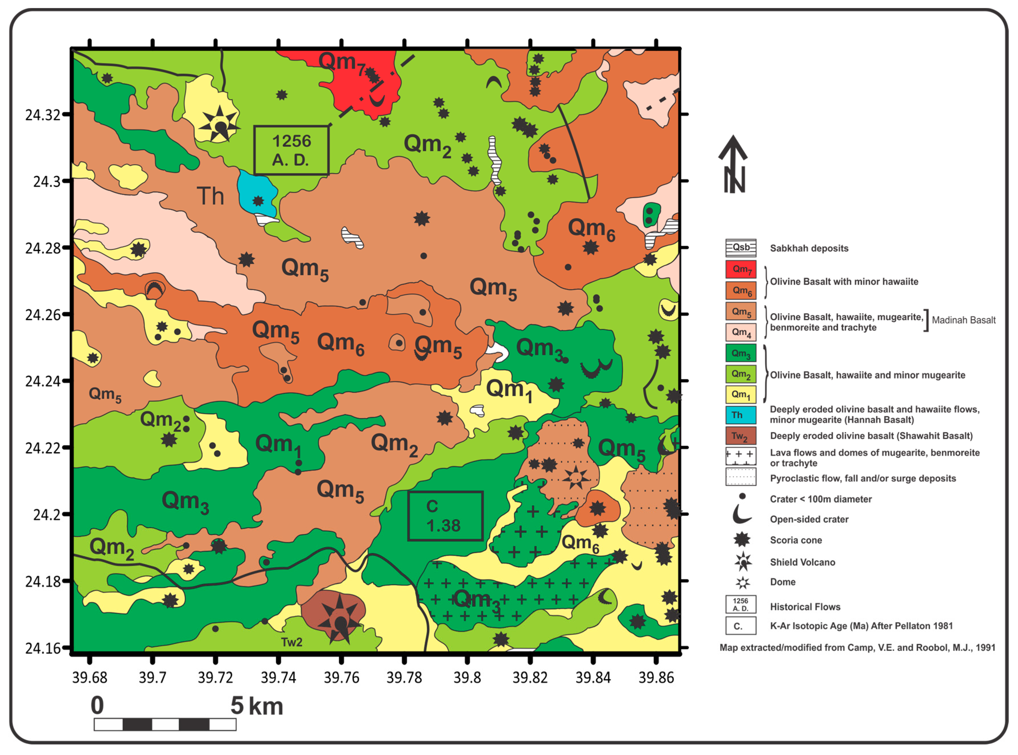
The study area is the northern part of the Rahat volcanic field (
Figure 1), the Cenozoic lava field in western Saudi Arabia. It is one of the largest volcanic fields on the western margin of the peninsula and a part of the Red Sea rift. At an approximate coverage area of 20,000 km
2, the Rahat evolution commenced at 10 Ma [
8] with 36 shield volcanoes, 644 scoria cones, and 24 domes [
9,
10,
11]. Harrat Rahat comprises over 900 exposed vents, including maars, cryptodomes, craters, and scoria cones. Among these, 289 vents are isolated by more recent volcanic deposits and have not been associated with the 234 distinct volcanic rock units identified through geological mapping [
12]. A recent investigation and mapping effort focused on 32 geologic units that erupted within the northern Rahat volcanic field (RVF) after 1 Ma [
13]. These units consist of mugearite, tholeiitic and continental basalts, hawaiites, and intraplate alkali (
Figure 2).
The RVF is elongated in an N–S direction of about 310 km in the direction of the Makkah–Madinah–Nafud (MMN) volcanic line and comprises four smaller harrats that form an elongated shield-like shape with noticeable linear vents in the central area [
9,
14].
The most recent volcanic event in the region occurred in 1256 A.D.; it is known as the Al-Madinah eruption or historical eruption and resulted in a 2.25 km long fissure eruption and the formation of a 23 km long lava flow east of Medina. There were earlier eruptions, such as in 641 CE, which made finger-like flows to the east of the 1256 A.D flow [
15], thus fueling concerns of reoccurrences in the near future. This volcanic field appears to be the biggest lava field in Saudi Arabia [
16]. In addition to these concerns, there has also been a recent increase in seismic activity in the region since 2009 [
17]. This significant 1256 A.D eruption lasted for 52 days, during which 0.5 km
3 of alkali olivine basalt was extruded from the fissure, leading to the creation of six scoria cones. The extensive lava flow reached a distance of nearly 8 km from the city of Al-Madinah. The erupted basaltic rocks encompass a diverse range, including alkaline olivine basalts to hawaiite, as well as olivine transitional basalts. Additionally, formations of Benmoreite, mugerarite, and trachyte are present in the form of tuff and lava flows. The Harrat Al-Madinah basalts are further categorized into lower and upper Al-Madinah Al-Munawwarah basalts, as documented by Camp et al. [
8]. This eruption event provides valuable insights into the geological history and volcanic activity of the region, shedding light on the complex processes associated with volcanic events in this area. Further details regarding the general geology in the study area are provided in Aboud et al. [
9], Alqahtani et al. [
10], Robinson and Downs [
12], Al-Amri et al. [
14], El-Hussain et al. [
18], and Moufti et al. [
19].
Figure 1.
Cenozoic lava fields of western Saudi Arabia with their distribution of ages (modified from [
9,
19]). The inserted yellow square portrays the study area.
Figure 1.
Cenozoic lava fields of western Saudi Arabia with their distribution of ages (modified from [
9,
19]). The inserted yellow square portrays the study area.
Figure 2.
Geology map of the region considered in this study (modified from [
10]).
Figure 2.
Geology map of the region considered in this study (modified from [
10]).
The RVF is of special interest owing to its proximity to the city of Al-Madinah al Munawwarah, which sits within, and is continuing to expand southward over, the north end of the volcanic field [
12]. Multiple volcanic vent systems exist within the study area (
Figure 3). Such settings have been considered as pointers to volcanic centers that host very large high-temperature reservoirs [
20]. The relationship between the number of volcanic vent and magma reservoir characteristics is not always a simple direct correlation. Some large reservoirs may have a low number of vents, while smaller reservoirs can sometimes have multiple vents. Nevertheless, multiple vents may often indicate a larger underlying magma reservoir system, and larger magma chambers typically have the capacity to feed multiple surface expressions [
21]. The depth and geometry of the reservoir may affect vent distribution just as local tectonics and stress field play major roles in vent formation. In addition, rock type and structural features influence how easily multiple pathways can form [
22]. An inversion of the gravity field data from northern Rahat [
23] indicated a wide depression of the basement surface. This depression appears deeper along the primary vent axis of the eastern and southwestern parts of the volcanic field. A less dense basement underneath the vent axis in the field was also identified and suggested to have arisen from lithological deviations in the basement that occurred prior to Cenozoic volcanism. In a series of fieldwork spanning through years 2014, 2015, 2016, and 2017, ref. [
12] successfully identified probable contacts between volcanic rocks and deposits through examination of shaded relief images produced from digital elevations and from satellite photographic images in a geographic information system (GIS). Mapped units were then characterized, correlated, and distinguished by thin-section petrographic, geochemical, paleomagnetic, and geochronologic studies.
Volcanic vents and eruptive fissures were delineated and characterized using a combination of advanced remote sensing methodologies and comprehensive field studies at Harrat Khaybar, located further north of Harrat Rahat (Alohali et al. [
24]). Their in-depth analysis unveiled the evolutionary history of Harrat Khaybar, revealing a progression through five distinct eruptive phases. Notably, the spatial distribution of vent locations exhibited a notable convergence towards the central axis, resulting in the formation of a prominent north–south (NS) trend. Furthermore, a concentrated cluster of vents was observed along the axis of the regional Makkah–Madinah–Nafud (MMN) line. Drawing from their research, the team derived estimations for the cumulative probabilities of at least one eruption occurring within Harrat Khaybar over the next 100 years. The calculated probabilities ranged from 1.09% to 16.3%, representing the lower and upper bounds, respectively, with the highest probabilities being centered within the region of the central axis. This insight provides valuable implications for understanding the volcanic activity and associated risks within the Harrat Khaybar region.
Runge et al. [
25] devised a statistical approach for identifying eruptive events from observable vents. Their methodology was evaluated using the 968 vents within the Harrat Rahat volcanic field, spanning from 10 Ma to 0.6 ka. Furthermore, they conducted an assessment to estimate the quantity of concealed vents within a substantial volcanic deposit in order to establish an enhanced spatial recurrence rate estimate. The study yielded an average temporal recurrence rate of 7.5 × 10
−5 events per year for eruptive events. With application of some geophysical techniques of tilt derivative, Euler deconvolution, and 2D modeling inversion, Aboud et al. [
26] analyzed gravity and aeromagnetic data from the northern part of the RVF. The outcomes of their study indicated that the thickness of the lava flows in the research area ranged from 100 m on the eastern and western sides to as much as 300–500 m in the central part.
Several geophysical studies ([
9,
10]) have also been conducted at the Rahat region for the purposes of investigating the geothermal potentials of the region. The objective of the present study is to leverage machine learning techniques to explore patterns and correlations within the magnetic data and discern potential indicators associated with the presence of volcanic vents. This study would contribute to addressing the critical need for improved volcanic hazard assessment and management, as well as the development of early warning systems.
2. Methodology
The magnetic data used in this study were extracted from a collection of aeromagnetic datasets from the periods of 1962 to 1983. Surveys were carried out over designated individual blocks with ground clearances set at 150, 300, and 500 m, employing a line spacing of approximately 800 m. Further information on the aeromagnetic data has been provided by Alqahtani et al. [
10] and Zahran et al. [
27].
Figure 3 shows the extracted aeromagnetic data covering the study area and also displays known vent locations. The slight mismatch in some vent locations between
Figure 2 and
Figure 3 likely arises due to differences in the data sources used to prepare the maps. The geological map (
Figure 2) was derived from some early geological surveys (1958–1963), while the vent locations on map (
Figure 3) were extracted from recent satellite imagery from the Saudi Geological Survey (2022). These sources may have different levels of accuracy or interpretations in terms of the precise locations of vents. Therefore, considering the vent boundaries, some vents might be represented as points in one map and as larger features (e.g., vent clusters or craters) in another, as seen in
Figure 2. This simplification or generalization could lead to apparent mismatches. The vent data on the general geology map may not have been updated to match recent satellite observations and geological studies. The vent locations depicted in
Figure 3, derived from high-resolution satellite imagery, are likely more reliable than those in
Figure 2 due to the inherent advantages of remote sensing. Satellite-derived data provide precise geospatial information, consistent coverage, and the ability to detect subtle volcanic features that may not be evident in older field surveys or geological maps. Furthermore, the alignment of these vents with gravity lows and other geological patterns supports their validity. While the slight discrepancies between
Figure 2 and
Figure 3 exist, the advanced techniques used to derive vent data in
Figure 3 make it a more robust dataset for predicting volcanic vent locations.
Machine learning techniques would be used to analyze the magnetic characteristics of known volcanic vent locations and to also make predictions about the likelihood of new volcanic vents present at other geographical coordinates. Multiple machine learning models were taken into account for this study. The criteria for consideration was based on available data and the complexity of the relationships between the features and target variable. The target variable was defined as the presence or absence of a new volcanic vent at specific geographical coordinates. This was represented as binary labels (1 for presence, 0 for absence). With the target variable definition, the model was trained using existing vents as positive examples and other non-vent locations as negative examples in order to learn the patterns associated with volcanic vent locations in the magnetic data.
It is often beneficial to experiment with multiple models and compare their performance using appropriate evaluation metrics to determine the most effective model for a specific investigation. In our study, we considered a range of machine learning models, each with its own strengths and suitability for different tasks and datasets. The models we focused on include:
Logistic Regression:
- -
A simple and interpretable model suitable for binary classification tasks.
- -
Provides the probability of the input belonging to a certain class.
- -
Can be extended to handle multi-class classifications.
Decision Trees and Random Forests:
- -
Capable of capturing non-linear relationships and interactions between features.
- -
Decision trees are easy to interpret and visualize.
- -
Random Forests are an ensemble of decision trees, providing improved generalization and robustness.
Gradient Boosting Machines (GBMs):
- -
Captures complex relationships in the data by combining multiple weak learners.
- -
Can handle non-linear relationships and interactions.
- -
Often provides high predictive accuracy.
Support Vector Machines (SVMs):
- -
Effective for binary classification tasks, especially when the decision boundary is non-linear and the feature space is high-dimensional.
- -
Can be extended to handle multi-class classification.
- -
Utilizes the concept of maximizing the margin to find the optimal decision boundary.
We recognize the importance of experimenting with multiple models and comparing their performance using appropriate evaluation metrics to determine the most effective model for our specific investigation. We plan to assess the models using common evaluation metrics such as accuracy, precision, recall, F1-score, and area under the ROC curve (AUC-ROC) for binary classification tasks. By comparing the performance of these models on our dataset, we aim to identify the most effective model based on the specific characteristics of our data and the goals of our study. Regression algorithms are a type of machine learning algorithm used to predict numerical values based on input data. The goal of regression is to find a mathematical relationship between the input features and the target variable that can be used to make accurate predictions on new, unseen data [
28].
Logistic regression, a supervised machine learning algorithm, excels in binary classification tasks by predicting the probability of a specific outcome, event, or observation. This model yields a binary or dichotomous outcome, offering two possible results, such as yes/no, 0/1, or true/false [
29].
Equation (1) represents logistic regression:
where
input value,
predicted output,
bias or intercept term,
coefficient for input (),
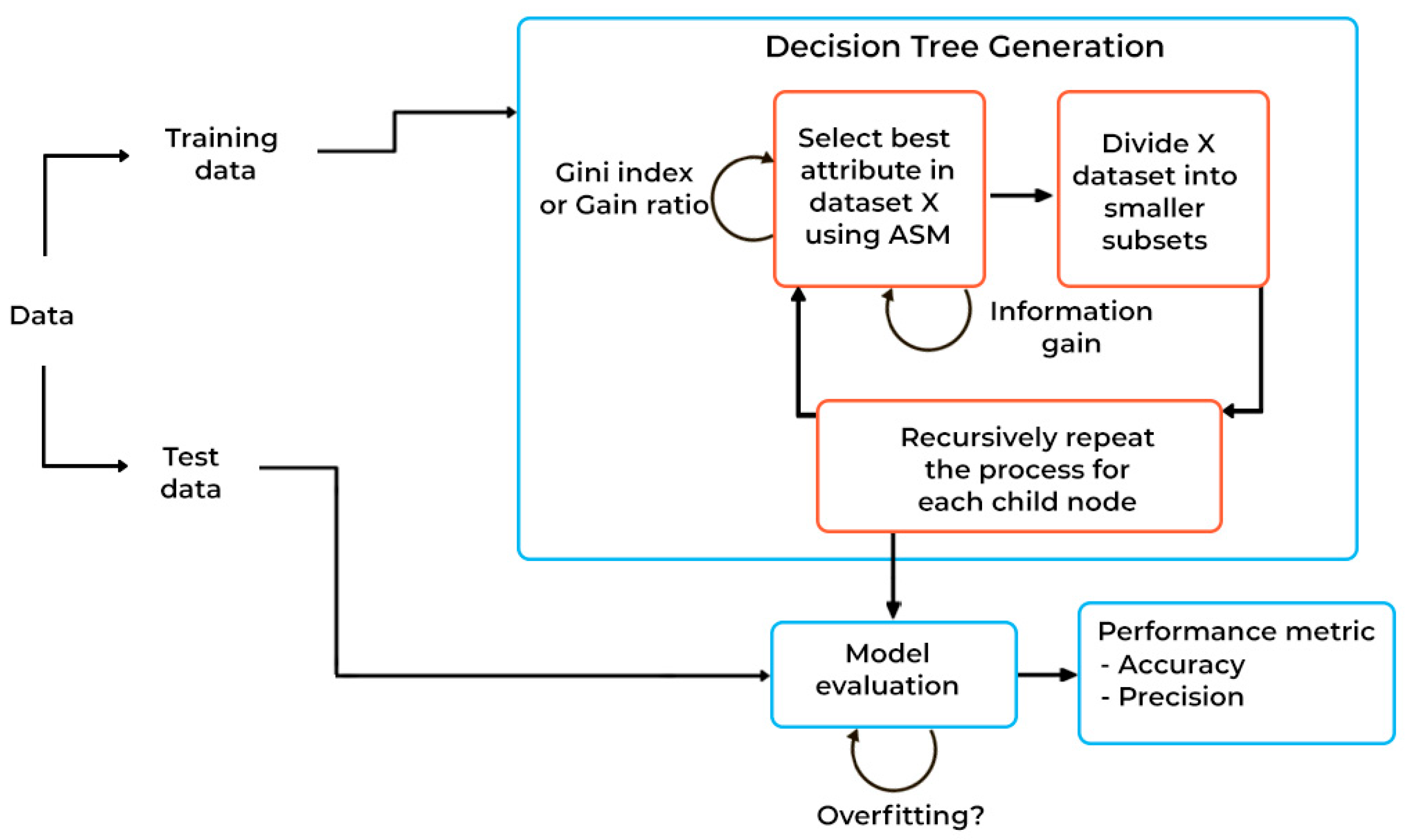
Decision trees: Supervised machine learning operations that model decisions, outcomes, and predictions using a flowchart-like tree structure. A demonstration of the basic decision tree flow chart is represented in
Figure 4.
The Gini index measures the chances or likelihood of a randomly selected data point misclassified by a particular node. The cost function for evaluating feature splits in a dataset is the Gini index. The Gini index is given by Equation (2);
where
p = probability of an object being classified to a particular class.
Attribute Selection Measure (ASM) is a technique used for selecting the best attribute for discrimination among tuples. It gives rank to each attribute, and the best attribute is selected as the splitting criterion. When considering decision trees, they aid in constructing a suitable tree for choosing the optimal splitter, with values typically ranging between 0 and 1.
Random Forest stands out as a highly potent machine learning model in predictive analytics, establishing itself as a cornerstone in industrial machine learning applications. This model operates as an additive model, leveraging a series of base models to make predictions effectively. For a new input data point, the Random Forest Regression model makes a prediction by aggregating the predictions of all the individual trees in the forest. The mathematical equation can be represented as:
where
the predicted output for the input data point ;
total number of trees in the Random Forest;
the prediction of Decision Tree for the input data point .
This equation represents the averaging of the predictions of all the individual trees in the Random Forest to obtain the final prediction for the input data point. For more on the Random Forest regression, see Breiman [
30].
A GBM, which integrates gradient descent into boosting, follows the same algorithm as gradient boosting. This decision tree-based model utilizes a gradient descent approach to determine the
(step size) for a tree with T leaves. To calculate
at, for example, iteration
m, and given several derivations in the region
(leaf
j), the basic equation for a GBM is [
31]:
where
is our model at iteration m, is the actual value, and L is the loss function.
SVMs: A binary SVM aims to classify subjects into one of two classes by utilizing specific features. The basic mathematical equation for Support Vector Machines (SVMs) can be described as follows:
Given a set of training data (x
1,y
1), (x
2,y
2), ..., (x
n,y
n), where xi represents the input features and yi represents the class labels (either −1 or
for binary classification), the goal of a SVM is to find the optimal hyperplane that separates the data into different classes while maximizing the margin. The equation for the decision function of a linear SVM can be represented as:
where
f(x) is the decision function that predicts the class of the input x;
w is the weight vector;
x is the input feature vector;
b is the bias term;
* represents the dot product.
The optimal hyperplane is determined by finding the weight vector w and the bias term b that maximize the margin while correctly classifying the training data. This is achieved by solving the optimization problem of maximizing the margin subject to the constraint so that the data are correctly classified. In the case of non-linear Support Vector Machines (SVMs), the process entails employing kernel functions to transform the input features into a higher-dimensional space. This transformation allows for the use of a linear hyperplane to effectively separate the classes. The mathematical formulations for the optimization problem and the utilization of kernel functions in non-linear SVMs are notably intricate, involving the principles of Lagrange multipliers and the dual form of the optimization problem. Further insights into SVMs are given by Vapnik [
32] and James et al. [
33].
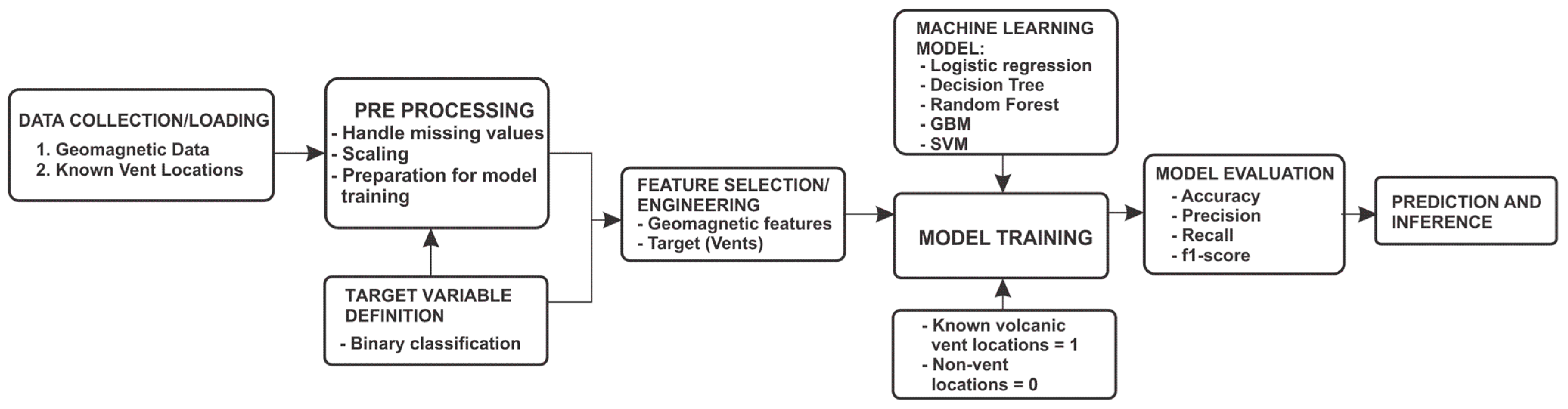
Concept Implementation
In this study, we used the following input data for the machine learning model:
Longitude: The geographic longitude of each data point, which provides spatial information relevant to the location of magnetic anomalies and volcanic vents.
Latitude: The geographic latitude of each data point, paired with longitude to give a complete spatial reference for the dataset.
Magnetic Anomaly: The measured magnetic field intensity at each data point. This value is critical for identifying subsurface geological features that may be associated with volcanic activity.
Vent Presence (Yes/No): A binary indicator that specifies whether a volcanic vent is present at the corresponding location. This variable serves as the target variable for the regression model, allowing us to train the model to recognize patterns associated with vent locations.
The concepts for implementation were as follows:
- -
Data Collection and Preprocessing: The magnetic data should include information about the longitude, latitude, and geomagnetic characteristics (magnetic field intensity) of known volcanic vent locations. Data from non-vent locations could also be included to provide a contrast for the model in order to learn the differences between vent and non-vent areas. The data would be preprocessed to handle missing values, scale the features, and prepare for model training.
- -
The target variable for the machine learning input would be defined as the presence or absence of a new volcanic vent at specific geographical coordinates.
- -
Feature Engineering—Geomagnetic Features: The geomagnetic data, including magnetic field intensity and other relevant characteristics, would serve as the features for the model (note: other relevant geographical or geological features could also be included, if available).
- -
Model Training—Training Data: The model would be trained using the known volcanic vent locations as positive examples (label 1) and non-vent locations as negative examples (label 0).
- -
We used a portion of the vent locations and magnetic field data for training and reserved a separate set for model evaluation to assess its performance reliably. Specifically, we applied an 80–20 split, where 80% of the data was randomly selected for training and the remaining 20% was used exclusively for testing.
Model Training—Machine Learning Model: A binary classification model, as with logistic regression, decision tree, Random Forest, GBM and SVM, was trained to learn the patterns associated with volcanic vent locations in the geomagnetic data.
To ensure that the model learned spatial patterns in the magnetic field data rather than simply memorizing the coordinates of known vents, we implemented several techniques. First, we applied a stratified k-fold cross-validation approach, ensuring that each fold included a diverse mix of vent and non-vent locations spread across different regions. This forced the model to generalize from patterns in the magnetic anomalies rather than focusing on specific vent coordinates. Additionally, we experimented with data augmentation by creating artificial spatial offsets in both the longitude and latitude. This technique introduced minor shifts to the magnetic field data while preserving underlying patterns, helping the model focus on features associated with vent presence rather than absolute positions.
We approximated each vent as a central point to simplify the modeling process, as the exact vent boundaries were not always clearly defined in the dataset. When multiple mesh nodes fell within the extent of a vent, we assigned a target value of 1 to all such nodes, treating them as being representative of the larger vent structure. This approach allowed the model to recognize the spatial extent of vents without requiring detailed boundary information.
Hyperparameters in machine learning are the configuration settings that are external to the model and are not learned from the data. These parameters are set prior to the training process and are used to control the learning process. For this study, the hyperparameters associated with the Random Forest algorithm are n_estimators (this hyperparameter determines the number of decision trees in the Random Forest; each tree in the forest is trained on a random subset of the training data, and n_estimators control how many of these trees are used in the ensemble), max_depth (this hyperparameter sets the maximum depth of each decision tree in the Random Forest, and controls the maximum number of levels in each decision tree, which can help prevent overfitting), min_samples_split (this hyperparameter sets the minimum number of samples required to split an internal node during the construction of a decision tree; it can help control the complexity of the model and prevent overfitting), min_samples_leaf (this hyperparameter sets the minimum number of samples required to be at a leaf node; it can also help control the complexity of the model and prevent overfitting), and bootstrap (this hyperparameter determines whether bootstrap samples are used when building trees; if set to True, each tree in the random forest is built on a bootstrap sample of the training data, which introduces randomness and helps prevent overfitting, and the depth of a decision tree). Therefore, to improve the performance of the machine learning model, model training and evaluations were performed with the best hyperparameters derived from tuning as follows: n_estimators (100, 200, 300), max_depth (10, 20, 30, None), min_samples_split (2, 5, 10), min_samples_leaf (1, 2, 4), and bootstrap (True, False).
- -
Prediction and Inference: Once the model was trained, it was used to make predictions about the likelihood of new volcanic vents being present at other geographical coordinates based on their geomagnetic characteristics. These predictions were used to identify potential areas for further investigation or monitoring for volcanic activity.
- -
Model Evaluation and Refinement: The model’s performance was evaluated using metrics such as accuracy, precision, recall, and F1-score.
- -
Make predictions using the trained Random Forest model.
The flowchart for application of concepts used in this study is shown in
Figure 5. Trained model was used to make predictions about the likelihood of new volcanic vents presence at other geographical coordinates given their magnetic characteristics.
4. Discussion
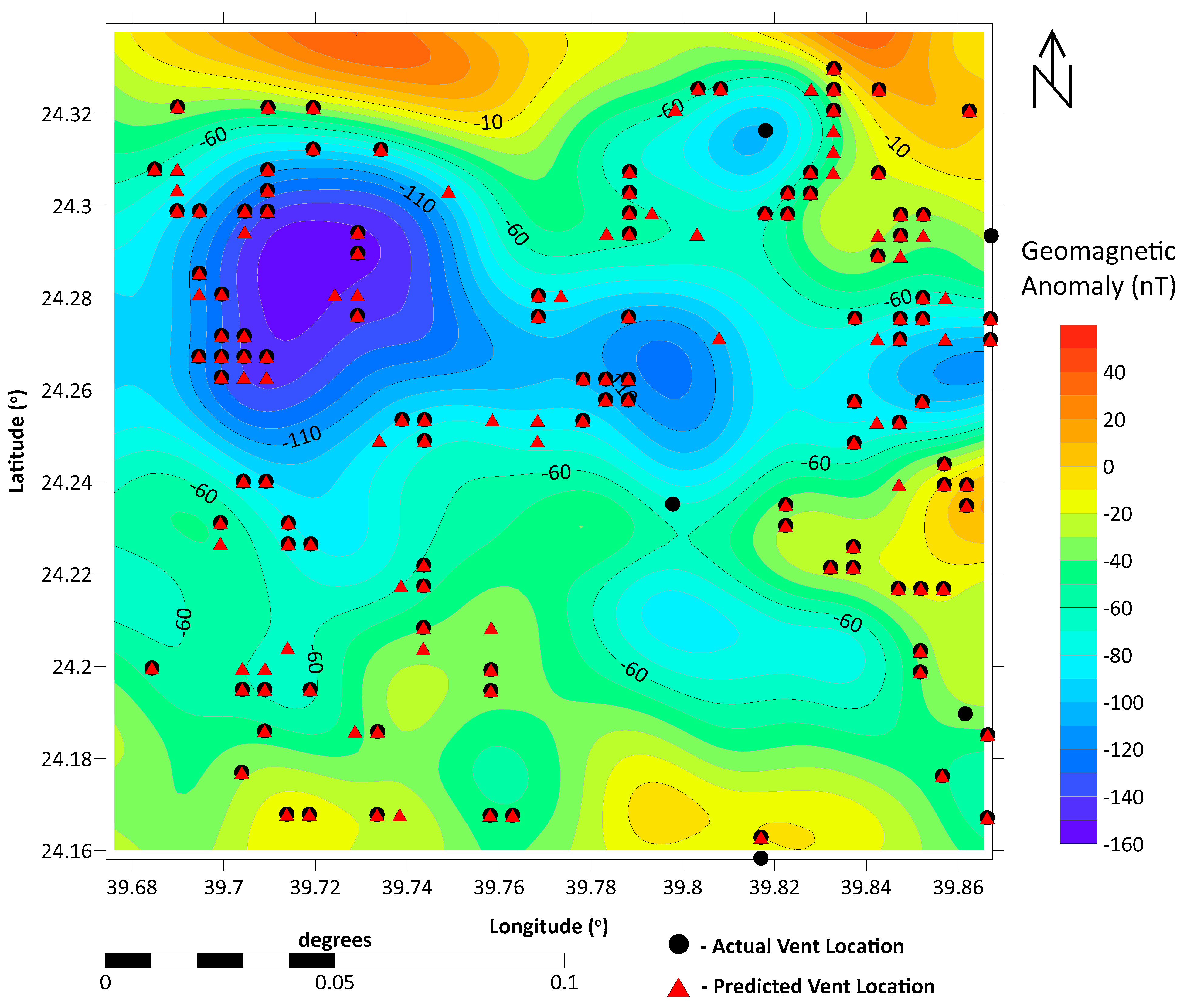
The analysis of the geological characteristics of the study area (
Figure 2) and the volcanic vent distribution across the magnetic dataset (
Figure 3) reveals a nuanced understanding of the region’s subsurface dynamics. The vent system exhibits a generally sparse distribution pattern; however, significant concentrations of vents are observed in specific geological formations and regions, providing key insights into the underlying geological and geophysical processes.
In the northern section of the research area, the presence of olivine basalt, hawaiite, mugearite, benmoreite, and trachyte formations within the Madinah Basalt is notable. This area emerges as a focal point with higher concentrations of vents, correlated with low magnetic anomalies (<−20 nT). These low anomalies suggest a complex subsurface structure, likely influenced by past volcanic and tectonic activities. The concentration of vents in these formations indicates a significant correlation between the geochemistry of the host rocks and the location of volcanic activity. This supports the hypothesis that the geochemical composition of these rocks plays a crucial role in the formation and distribution of volcanic vents. In addition to the northern area, denser vent concentrations are also observed in the eastern and central regions of the study area, corresponding to low magnetic anomalies (<−10 nT). Alqhatani et al. [
10] and Berthier et al. [
35] have characterized these regions, particularly those situated on olivine basalt, as being indicative of an abnormal subsurface body with potential geothermal resources. This abnormality could be the result of past volcanic activities or geothermal processes, aligning well with the observed magnetic anomalies.
Conversely, the southern region displays a sparser distribution of vents and is primarily associated with olivine basalt formations. This pattern may indicate less volcanic activity or different subsurface conditions that are less conducive to vent formation. The variability in vent distribution across the study area highlights the influence of geological and geophysical factors in volcanic activity. The observed volcanic vents (
Figure 3) are predominantly concentrated within the anomalous body identified by the magnetic data, indicating a strong correlation between vent distribution and subsurface geological anomalies. In northern Harrat Rahat, approximately 900 constructional vents, including scoria cones and spatter ramparts, are visible. Among these, 289 have been enclosed by more recent lava flows, effectively isolating them from their associated effusive products [
12].
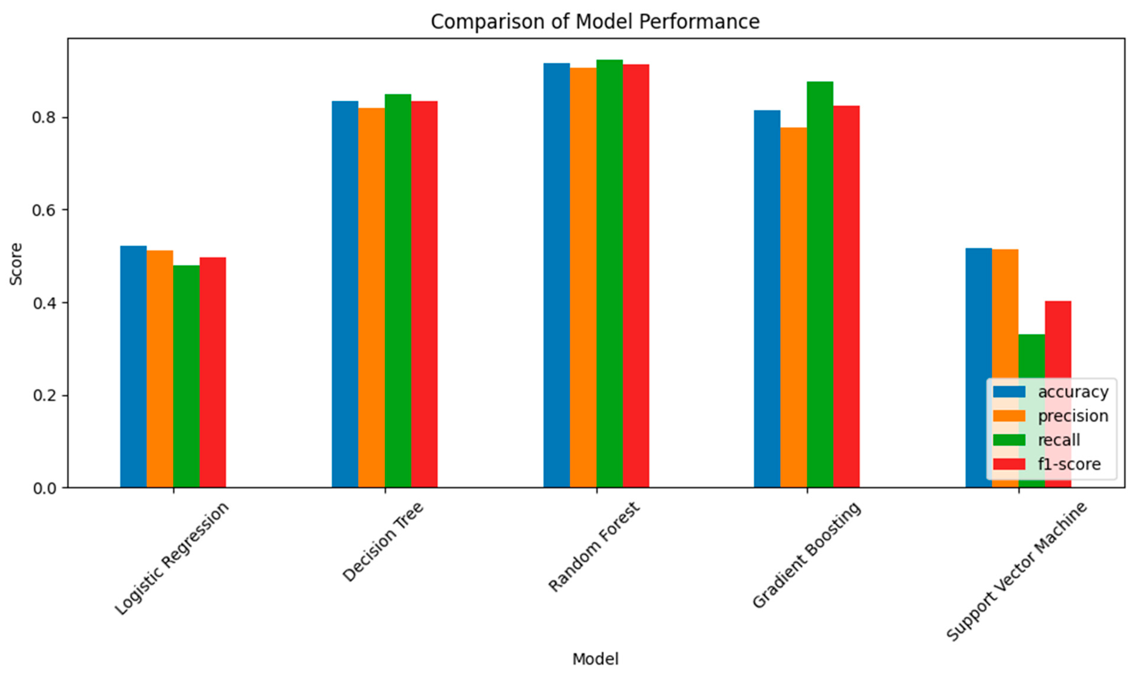
The selection of the optimal machine learning model for predicting vent locations was guided by factors such as dataset size, data complexity, and model interpretability.
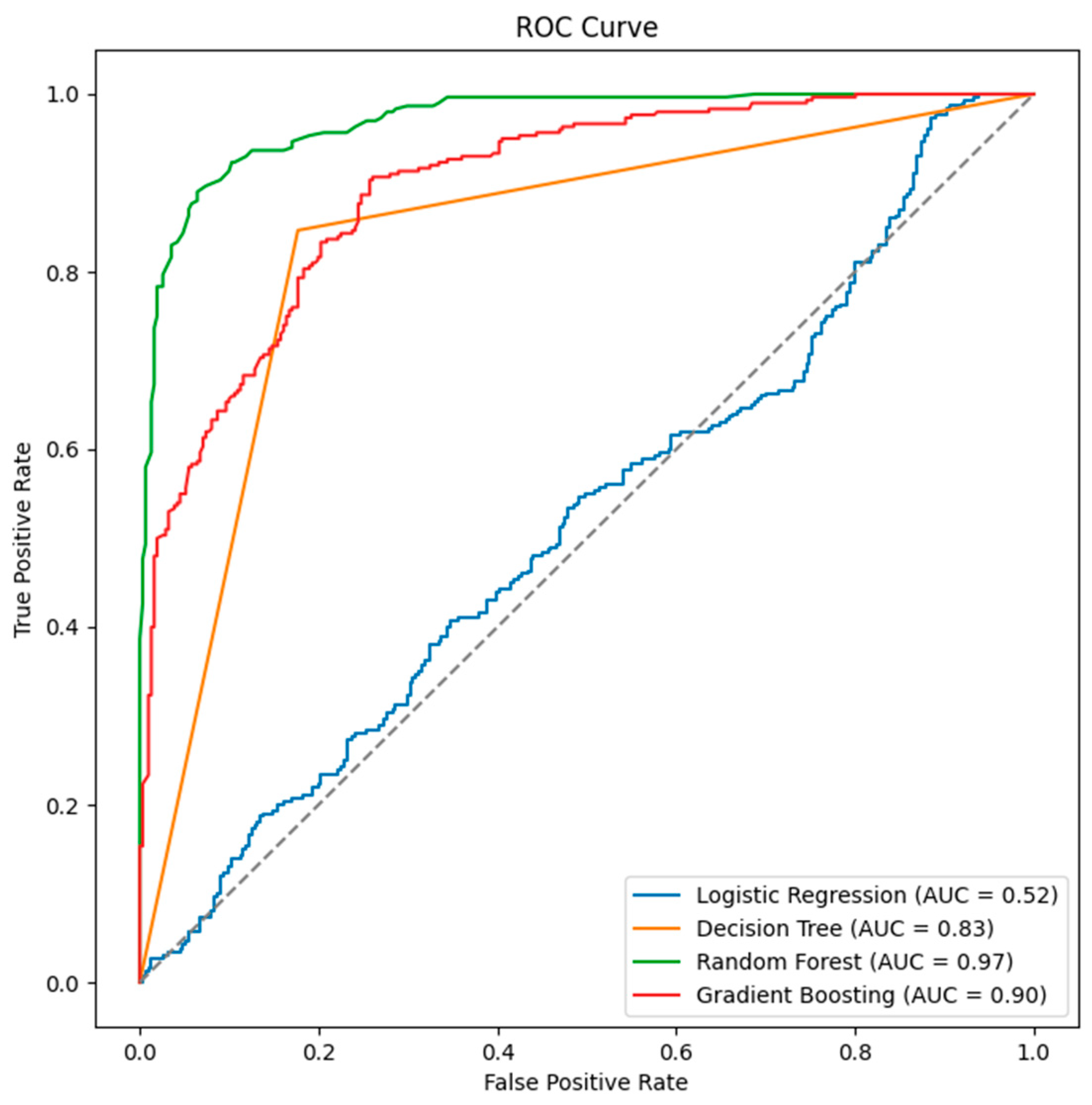
Table 1 compares the adopted models and their performance metrics. Among the models tested, the Random Forest model demonstrates the highest accuracy, precision, recall, and F1-score. Its robust performance metrics and ability to handle data imbalances make it the preferred choice for further optimization and fine-tuning. The model performance plot (
Figure 6), ROC curve, and AUC evaluations (
Figure 7) confirm the selection of the Random Forest classifier, with an AUC value of 0.97 indicating superior performance in differentiating between positive and negative classes.
The predicted vent locations (
Figure 8) show a satisfactory alignment with the actual vent locations and identify additional potential vent sites. The predicted vents are distributed across the study area, with significant additions in the northern region, likely linked to the observed dense vent distribution. This suggests that some predicted vents might be concealed beneath the surface, obscured by volcanic eruptive deposits or structural changes such as faulting, subsidence, or uplift. During previous eruptions, volcanic vents could have been covered by lava flows, pyroclastic flows, and ash, concealing the original vent openings. The dated and mapped volcanic deposits of northern Harrat Rahat have been assigned to 12 eruptive stages [
36], with the resolutions of older stages being poor due to concealment by younger volcanic products and erosion. This has resulted in some older map units being composites from multiple eruptions [
12].
Figure 9 shows a superimposed plot of the predicted vent locations on the actual vent locations, facilitating direct comparison. The new predicted vent locations are represented as red triangles, while those predicted at exact locations of the actual vents (black dots) are superimposed on the actual vent locations. Significant predictions were observed in the northern, northeastern, northwestern, and central regions, with fewer predictions in the southwestern regions. The correlation between actual and predicted vent locations is 86%, with a Degree of Certainty (DC) of 97%.
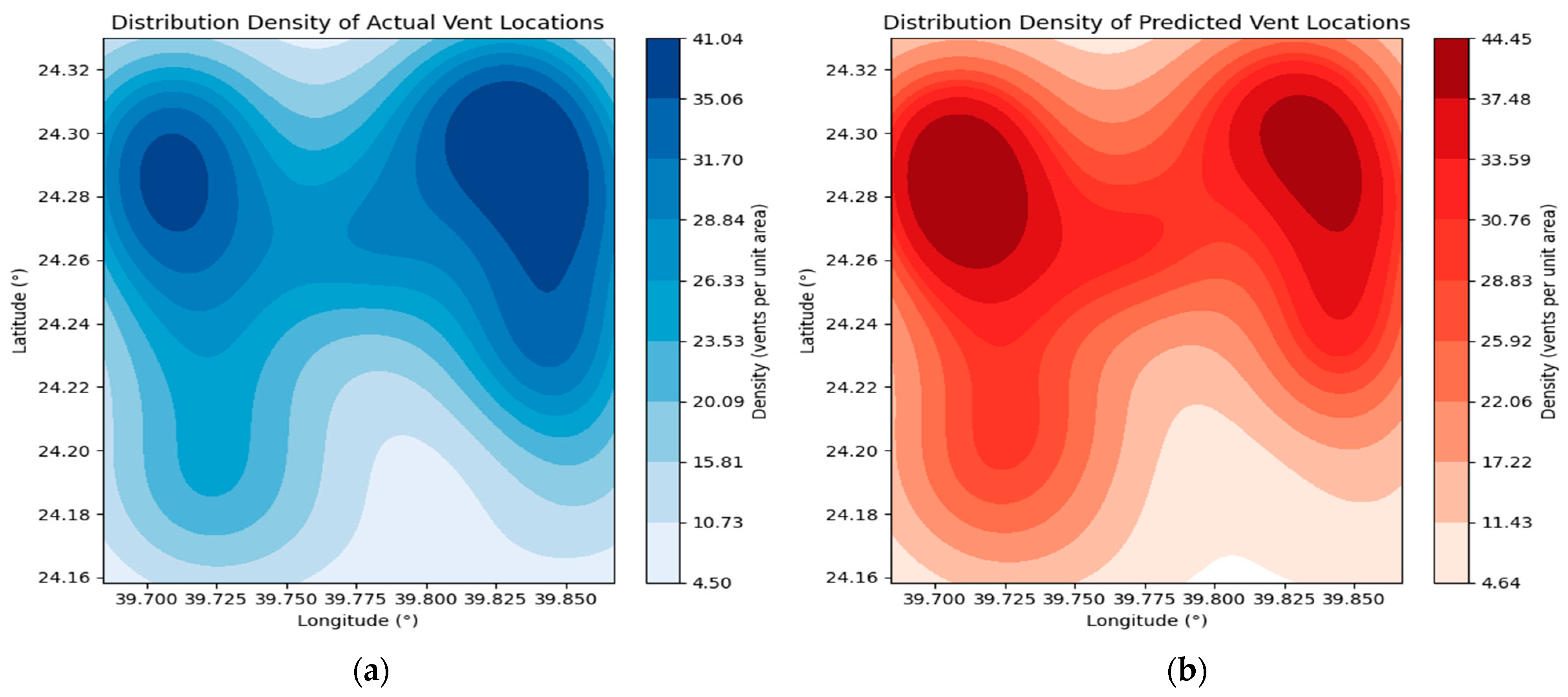
Figure 10 depicts the spatial distribution of known vent locations, with color intensity representing vent density in different areas. Comparing
Figure 10a,b shows similar density patterns in the same geographic areas, supporting the model’s performance. The predicted vent density closely matches the actual vent density, suggesting the model’s effectiveness in capturing the spatial patterns of vent locations.
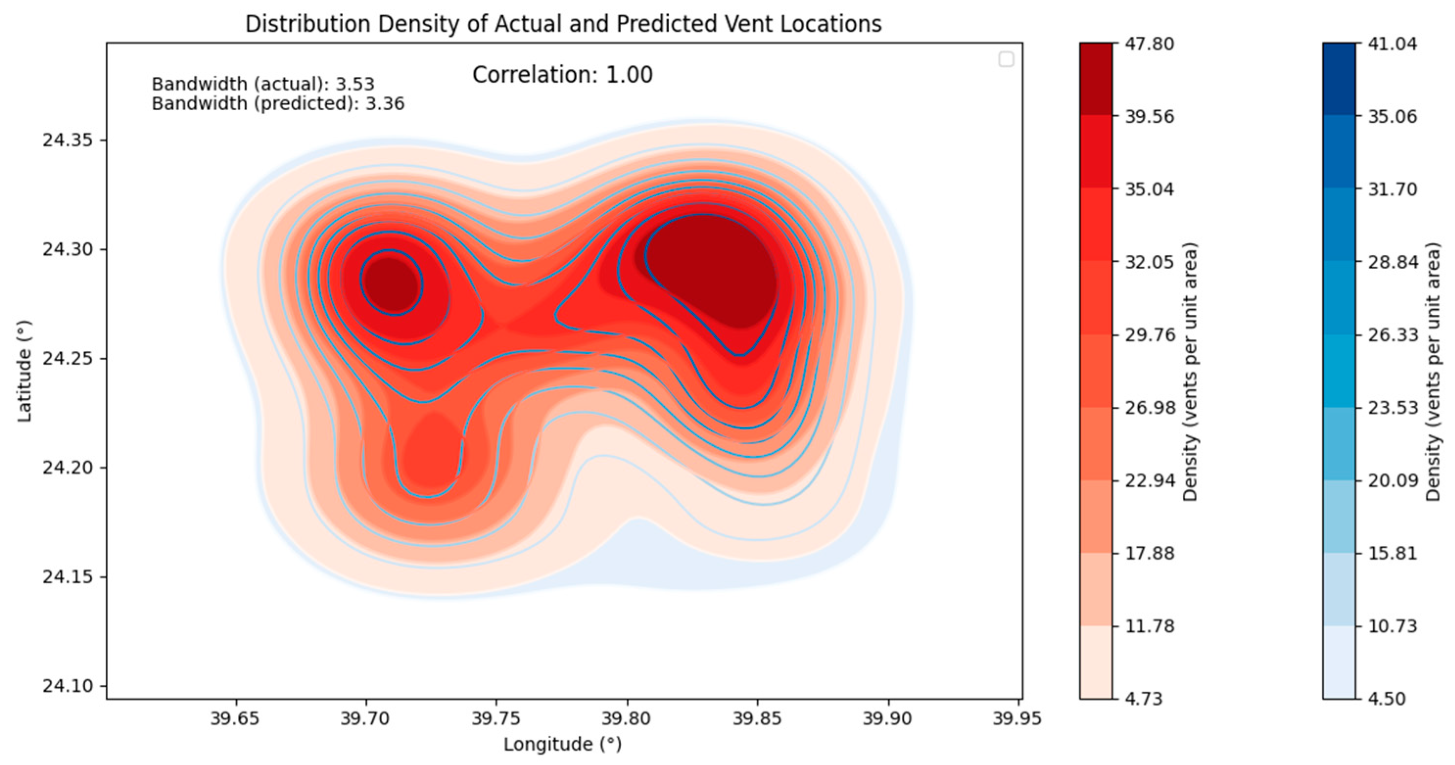
Figure 11 provides a correlation measure between the two distributions with a correlation coefficient of 1, indicating a strong positive correlation. This high correlation validates the model’s predictions and its ability to identify vent locations accurately. This study quantitatively assesses the similarity between the distribution densities of actual and predicted vent locations. The insights gained from the correlation between magnetic anomalies and vent distribution provide valuable information for further geological and geophysical investigations.


