Assessing Shallow Groundwater Quality Around the Sheba Leather Tannery Area, Wikro, North Ethiopia: A Geophysical and Hydrochemical Study

Abstract

This study aimed to investigate the shallow groundwater status around the Sheba Leather Tannery area, Wikro, North Ethiopia, through geophysical and hydrochemical methods. Seventeen Vertical Electrical Soundings (VESs) acquisitions, 4 upstream and 13 downstream, of the leather tannery area were conducted. Using the data, four geoelectric profiles were generated. The aquifers’ geoelectrical layers, depth, and lateral extent were delineated. The VES curves depicted three to four resistivity layers. These alternating layers of low, moderate, and high resistivity values, traced at different VES points, were attributed to the formations’ composition and the groundwater quality status. Besides the geophysical survey, 32 water samples were collected from the area. Parameters such as electrical conductivity (EC), total dissolved solids (TDSs), pH, major ions, and heavy metals were analyzed. Moreover, PHREEQC was used to determine the groundwater mineral saturation indices where most minerals, except halite, were found supersaturated. The quality status for drinking purposes was also evaluated using the water quality index (WQI), and the water was classified as good (56.3%), poor (37.5%), and very poor (6.2%). The sodium adsorption ratio (SAR) and the percentage of sodium (Na⁺%) were calculated, and the results indicated that the water is suitable for direct use in irrigation.

1. Introduction

The leather industry plays a significant role in the economies of many developing countries. However, the discharge of highly toxic and carcinogenic chemicals in the tannery area as waste poses a substantial environmental threat [1,2,3,4,5,6]. The release of wastewater from leather factories can have detrimental effects on land use and the overall hydrogeochemical composition [7,8,9,10]. The impact of tanneries’ effluents on both surface and groundwater has been extensively studied worldwide, and these effluents cause significant physical and chemical changes in surface and groundwater, thereby leading to environmental degradation [11,12,13,14,15,16,17,18,19,20].

The Sheba Leather Tannery area in Wikro, located approximately 45 km north of Mekelle (Tigray region capital city), was the sole modern leather industry in the region. This industry, known for processing 6000 hides a day [21], has had inadequate wastewater treatment mechanisms and discharged approximately 120 m³ of tannery area wastewater daily [22]. The discharged wastewater contains chromium, sodium, calcium, magnesium, chloride, and sulfate, which pose a potential pollution threat. Several researchers have reported on the production capacity and a limited list of chemicals (chrome salt, sodium sulfide, sodium hydrogen sulfide, calcium hydroxide, and magnesium hydroxide) used in the plant, which had a critical impact on the environment [22,23,24]. The nearby streams and rivers surrounding the tannery area (Figure 1(C1,C2)) are particularly susceptible to pollution. The impact of this pollution could extend to a wider area as these streams and rivers drain a larger region and travel a considerable distance before joining the Geba River, which supplies/feeds water to the dam reservoir (under construction), which is planned to be the main water supply source to Mekelle city, the capital city of the Tigray region, with close to 700,000 people. The discharge of tannery area effluents can also have adverse effects on groundwater resources. In regions like Wikro and its surroundings, groundwater is the primary source of drinking water, and agricultural irrigation, as is the case in many parts of the world. In arid and semi-arid climates, such as northern Ethiopia, where precipitation and surface water are limited, groundwater plays a crucial role as a main resource [25,26,27].

Several significant preliminary investigations have been conducted at the Sheba Leather Tannery area, focusing on the impact of waste disposal on the natural environment and irrigation. These studies were carried out by various researchers, employing different methods to assess the extent of the tannery area’s environmental impact [21,22,23,24].

In 2011, a surface and groundwater sampling campaign was conducted to assess the concentration of heavy metals in the groundwater surrounding the Sheba Leather tannery area [24]. The results indicated that most of the heavy metal concentrations were below the laboratory detection limit, particularly chromium, iron, copper, arsenic, lead, and zinc, except for the samples collected from the wastewater disposal pond [24]. However, subsequent studies conducted a few years later reported higher concentrations of these elements that were previously considered very low or below the detection limit [23]. An initial geophysical investigation conducted by [24] aimed to evaluate the impact of the tannery area on the water resources. However, this investigation was limited to six Vertical Electrical Soundings (VESs), which were aligned along one dimension following the stream path. The spatial distribution of the VES points did not provide a comprehensive assessment of the area’s three-dimensional aquifer extent and contamination status. Additionally, due to the war in the region that began in November 2020, the Sheba Leather tannery area has suffered damage and vandalism. As a result, waste and stored chemicals were unmonitored and released into the environment. Hence, the water quality status of the study area needs to be evaluated. The water quality index (WQI) is a vital tool for assessing water quality, providing a simplified and standardized approach to evaluate and communicate its status [28,29,30,31]. It is commonly used in environmental monitoring and management studies to assess water resources for various purposes, including drinking, irrigation, and ecosystem health. In our study area, as well as in many developing countries, the application of the WQI tool is important due to the challenges these regions encounter in managing water resources and public health. Therefore, the primary goal of the current study is to investigate the current shallow groundwater quality status and hydrochemical properties near the Sheba Leather tannery area in the Wikro area in Tigray.

To achieve this, an integrated approach combining geophysical, hydrogeological, and hydrochemical methods was utilized. Each method offered specific insights, and their combined application enhanced the overall understanding of the hydrological and chemical processes occurring in the subsurface. The geophysical technique effectively identifies and maps changes in resistivity that may be due to contamination, while the hydrochemical analyses detect specific pollutants and their concentrations. By combining these approaches, decision-making regarding pollution management and mitigation can be significantly improved. The current assessment approach aids in making informed decisions about the general drinking water supply and agricultural practices in the study area and elsewhere.

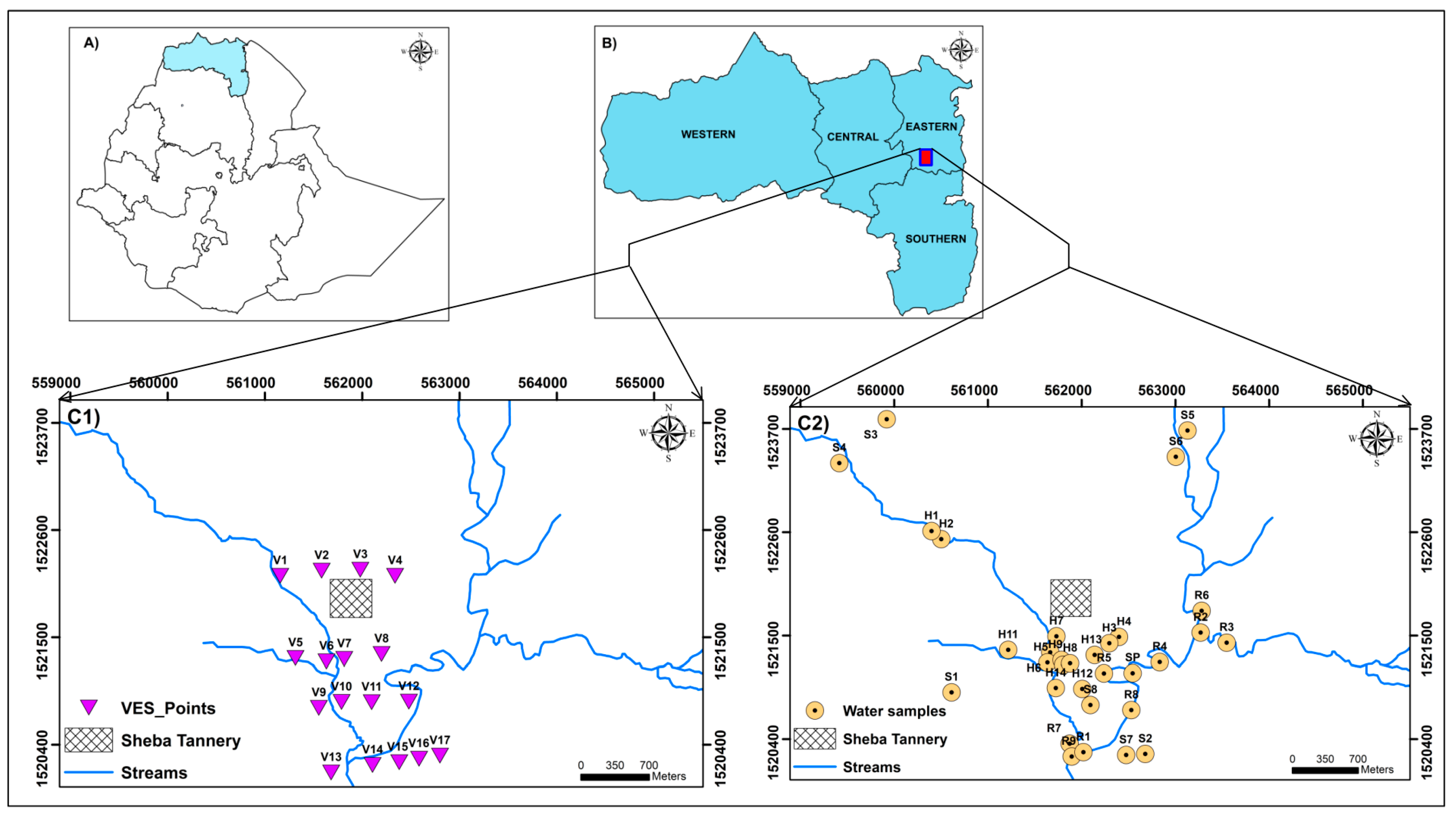
2. Study Area Description

The Sheba Leather tannery area is situated southwest of Wikro, approximately 45 km away from Mekelle, which is the capital city of Tigray. The study area falls within the Genfel sub-catchment and is positioned upstream of the confluence of the Upper Geba catchment. The dominant drainage pattern in this region is the dendritic type. With a semi-arid climate, the rainy season typically spans from early June to mid-September. Meteoric water serves as the primary source of natural recharge for the aquifers in the area.

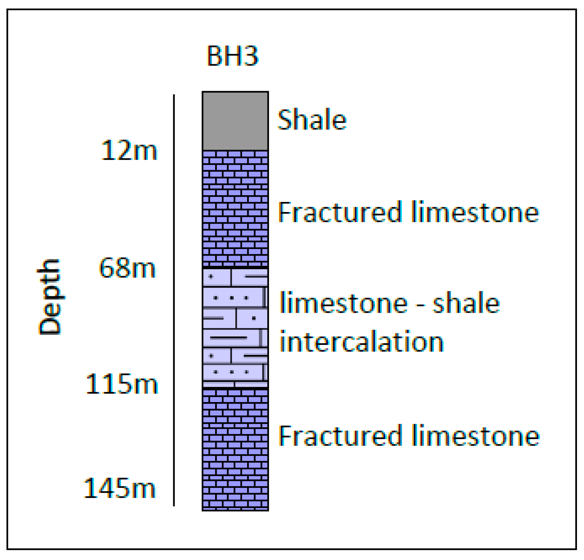
3. Geological and Hydrogeological Settings

The regional geological setting belongs to the northern Ethiopia geology. North Ethiopia’s geology comprises rocks formed during the Neoproterozoic, Paleozoic–Mesozoic, and Cretaceous periods [32,33,34]. The lithological and structural setup of the study area is part of the Mekelle sedimentary basin. These sedimentary rock successions are surrounded by metamorphic rocks with various mineralogical compositions and structures, which define the geology of the Wikro area [34,35]. The rock types are regionally grouped, with names derived from localities where they are dominantly found, such as Edaga-Arbi tillite, Enticho sandstone, Adigrat sandstone, Antalo limestone, and Agula shale [36].

The Negash geosynclinal fold and the Wikro fault zone found in this area are well-known Neoproterozoic and Cenozoic structures, respectively, in northern Ethiopian geology [34,35,37,38].

The rock types found in the Wikro area have been mapped (Figure 2). The Enticho sandstone and Edaga-Arbi tillites, collectively called the Paleozoic deposits, cover a very small area and are not shown separately on our map due to their scale. The Edaga-Arbi tillite has variable thicknesses across locations within the context of northern Ethiopia’s geology [36]. Boulders and poorly sorted sediments are the defining features. Overlying the Edaga-Arbi tillite/Enticho sandstone is the Adigrat sandstone, characterized by different kinds of cross-bedding structures [36]. This sandstone’s predominant cementing material is iron hydroxide, which gives a reddish color to the unit due to weathering. The limestone rock unit, named as Antalo limestone formation, exhibits a flawless bedding structure and has significant area coverage. The majority of the central area is covered with the Agula shale, including the entire city of Wikro and the Sheba Leather tannery area. This geological unit is the youngest of all the Mesozoic epoch sedimentary rock successions [36] in the area.

The research area lies in a structurally complex region: the Neoproterozoic shear fractures and the Cenozoic extensional fractures are likely to have considerable significance in recharge and groundwater resource development. Prominent fractures that have WNW-ESE and NNW-SSE orientations of a narrowly spaced long continuity and vertical dip make up the Wikro fault zone. A NNE-SSW running major dike-injected fracture passes east of the Sheba tannery area and dissects many of the Wikro faults. Three deep boreholes with depths of 120 m (BH1), 125 m (BH2), and 145 m (BH3) were drilled in the area. The lithological log of the deep borehole BH3 is shown in Figure 3. Evidence from the three borehole lithological logs indicates that limestone, shale, limestone–shale intercalation, and sandstone are the main geological formations, with fractured limestone serving as the primary groundwater-bearing zone. The productive and exploitable aquifers in this area are predominantly the highly fractured limestones. The aquifer thicknesses determined from the three boreholes are 45 m, 48 m, and 38 m, respectively. Moreover, the static water levels recorded during drilling were 17.8 m, 37 m, and 10 m, respectively. The groundwater conditions and flow regimes are believed to be influenced by regional and local geological structures.

4. Materials and Methods

4.1. Geophysical Survey Using Vertical Electrical Soundings (VES)

This study, similar to other researches conducted in different parts of the globe [39,40,41,42,43,44,45,46], used a geophysical survey, specifically Vertical Electrical Sounding (VES) was employed to determine the electrical resistivity of the subsurface. The VES method involves injecting electric currents into the ground via two current electrodes. The potential difference between two other electrodes (potential electrodes) is then measured. The apparent ground resistivity is calculated by applying Ohm’s Law, taking into account the distance between the electrodes, the applied current, and the measured potential difference. The variation in apparent resistivity values obtained through this method can provide insights into the nature of subsurface materials, including their degree of saturation and groundwater quality/salinity [47,48,49].

The VES method has been applied to the investigation of groundwater-bearing formations and associated environmental studies in different parts of the world [50,51,52,53]. It has also been an effective tool for subsurface layer characterization and groundwater resource pollution evaluations [41,54]. In this research, the Schlumberger array, with a maximum electrode separation AB/2 of 330 m, was used to carry out the VES survey. A total of 17 VESs (see Figure 1(C1)) were performed and compiled into four different profiles. The data were collected using a geophysical Terrameter (SAS 1000), and the IPI2win program was used for processing the raw data, inverse modeling, and generating cross-sections and profiles of the resistivity of the subsurface. During the interpretation of the resistivity sections, a correlation was made with the available boreholes and shallow wells lithological log data, where the actual geologic boundaries and lithological descriptions were compared to resistivity layers.

4.2. Water Samples, Analyses, and Suitability Parameters

To assess the shallow groundwater quality status and to identify potential contaminants, a total of 32 water samples were collected from 8 shallow wells, 14 hand-dug wells, 9 river waters, and 1 spring based on their availability and accessibility. The depth range for shallow wells is from 15 m to 60 m, while that of hand-dug wells ranges from 2 m to 10 m. Out of these 32 water samples, 4 shallow wells (S3, S4, S5, and S6) and 2 hand-dug wells (H1 and H2) were collected from the upstream side of the Sheba tannery area (Figure 1(C2)).

The sampling technique used conventional water sampling procedures [55]. EC, temperature, and pH were measured using a multiparameter probe. The samples were further analyzed at the water analysis lab using the industry-standard water quality analysis method [55]. Major anions were determined using UV spectrophotometry, while atomic absorption spectrometry (AAS) was used for major cations and trace elements analysis. The hydrogeochemical processes were evaluated using a scatter cross-plot and a multivariate statistical method. For the hydrochemical facies, a Piper diagram [56] was used, and the mineral saturation index (SI) was calculated using Phreeqc [57]. The SI indicates whether the minerals that come into contact with the water dissolve in it or precipitate out from it. A positive SI indicates oversaturation, implying that the water has a higher concentration of concerned dissolved ions than it can hold in a solution. A negative SI indicates undersaturation, meaning the water can dissolve more of a particular mineral. A zero SI indicates equilibrium, where the water is neither oversaturated nor undersaturated concerning a given mineral. Moreover, to evaluate the status and suitability of the shallow groundwater for various applications in the study area, parameters such as the water quality index (WQI), Na⁺ adsorption ratio (SAR), and Na⁺ percentage (Na⁺%) were evaluated.

The water quality index, a measure of the combined impact of many water quality parameters on the overall water quality, was calculated from the hydrochemical data. The calculated WQI was then further categorized using national and international water quality standards [58]. Twelve water quality parameters (

Table 1. Weights and relative weights to calculate the WQI.

Parameters	Standards [58]	Weight of Each Parameter (wi)	Relative Weight (Wi)
pH	6.5–8.5	4	0.09
Iron	0.5 mg/L	3	0.07
Calcium	75 mg/L	2	0.04
Magnesium	100 mg/L	1	0.02
Potassium	1.5 mg/L	2	0.04
TDS	1000 mg/L	4	0.09
Turbidity	5 NTU	3	0.07
Alkalinity	200 mg/L	4	0.09
Nitrate	50 mg/L	5	0.12
Sulfate	250 mg/L	5	0.12
Chloride	250 mg/L	3	0.07
Fluoride	1.5 mg/L	5	0.12
Total		41	0.94

) were taken to calculate the index for each sample using the weighted arithmetical index method. Maximum weights were given for sulfate, nitrate, and fluoride because these substances can cause serious human health impacts when they are at a high concentration [59,60,61,62,63,64,65], and minimum weight was given to calcium, magnesium, and potassium due to their lower importance in water quality evaluation [60]. Moreover, the assigned weights for these twelve water quality parameters took into consideration the local possible sources for the specific chemicals that can cause pollution, like agricultural activities, industrial effluents, and sewage discharges. The three steps for calculating WQI [66] are as follows: (I) choosing the parameters based on the data; (II) applying Equations (1) and (2) calculating the weighted arithmetic index (Wi) and the quality rating scale for each parameter; and (iii) the summation of the parameters using Equation (3).

$$\mathrm{W}\mathrm{i}={\displaystyle \frac{\mathrm{w}\mathrm{i}}{{\sum }_{\mathrm{i}=1}^{\mathrm{n}}\left(\mathrm{w}\mathrm{i}\right)}}$$

(1)

Qi = Vi/Si × 100

(2)

$$\mathrm{W}\mathrm{Q}\mathrm{I}=\sum \left(\mathrm{W}\mathrm{i}·\mathrm{Q}\mathrm{i}\right)$$

(3)

where Wi represents the relative weight, and “wi” represents the weight of each parameter according to its importance; “i” is the sample index; “n” is the number of hydrochemical parameters; “Qi” is the quality index; “Vi” is the monitored value for each parameter; and “Si” is the drinking water standard value [58] for each parameter. The WQI was used to evaluate the water’s suitability for drinking. The analyzed water samples were classified according to the World Health Organization [58] as excellent (WQI < 50), good (≥50 WQI < 100), poor (≥100 WQI < 200), and very poor (≥200 WQI < 300).

The water quality assessment and its suitability for irrigation were evaluated using SAR [64,67] and Na⁺% [64,68] using Equations (4) and (5), respectively. The Na⁺% is defined by [69] in Equation (5).

$$\mathrm{S}\mathrm{A}\mathrm{R}={\displaystyle \frac{{[\mathrm{N}\mathrm{a}}^{+}]}{\sqrt{\frac{{[\mathrm{C}\mathrm{a}}^{2+}+{\mathrm{M}\mathrm{g}}^{2+}]}{2}}}}$$

(4)

$$\mathrm{\%}{\mathrm{N}\mathrm{a}}^{+}={\displaystyle \frac{{(\mathrm{N}\mathrm{a}}^{+}+{\mathrm{K}}^{+})}{({\mathrm{N}\mathrm{a}}^{+}+{\mathrm{K}}^{+}+{\mathrm{C}\mathrm{a}}^{2+}+{\mathrm{M}\mathrm{g}}^{2+})}}\times 100$$

(5)

5. Results and Discussion

5.1. Geophysical Resistivity Survey

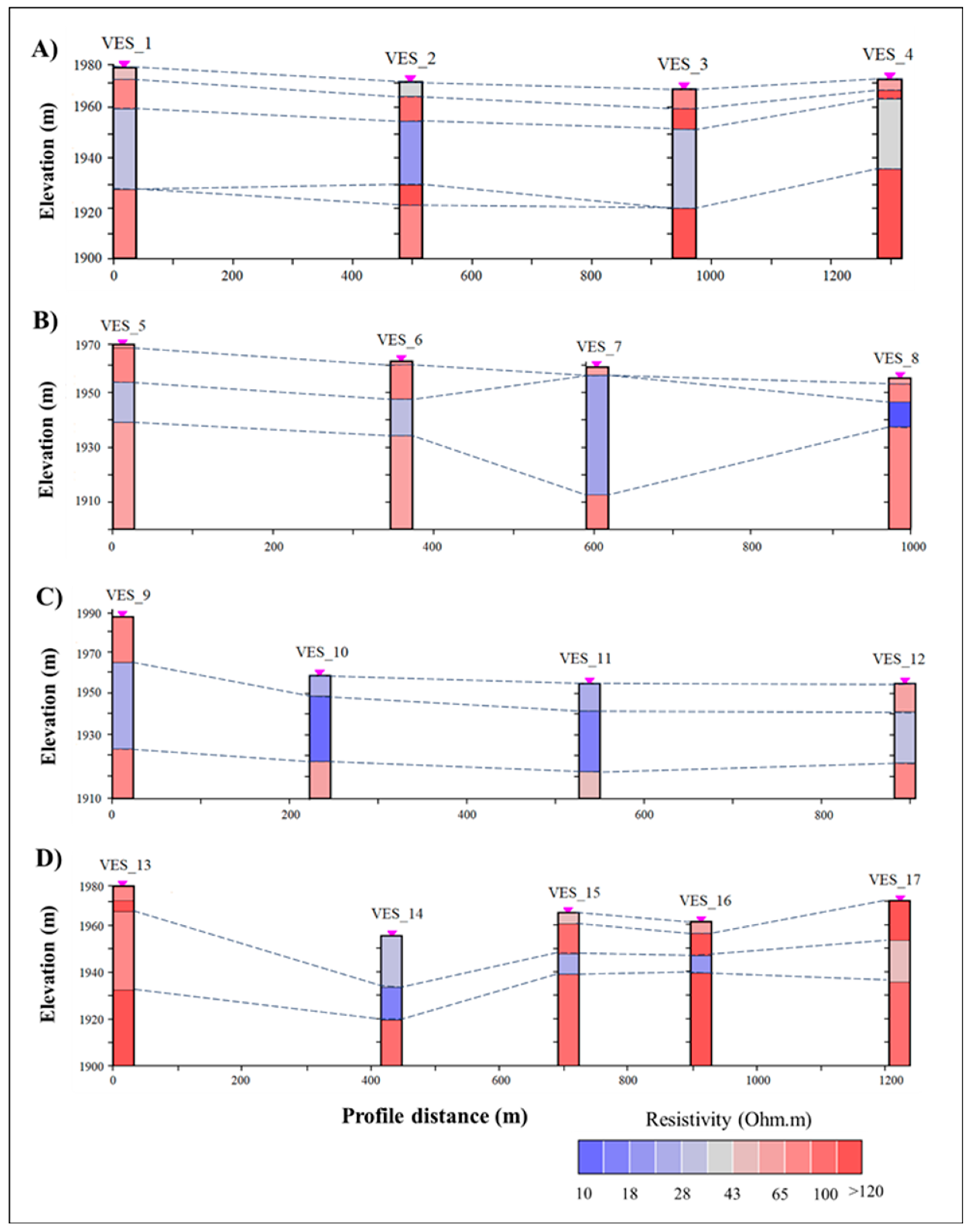
5.1.1. The Subsurface Resistivity Model of the Study Area

The VES results obtained from resistivity sections (VES_1 to VES_17) were used to delineate the lateral and vertical variations in the subsurface of the study area. By inverting the VES curves, model layer thicknesses and resistivity values corresponding to different hydrogeological units were derived. The three deep wells (BH1, BH2, and BH3) drilled in the city of Wikro near the Sheba leather tannery area, discussed in detail in the hydrogeological section (See Section 3) and illustrated in the geological map (Figure 2), were analyzed to interpret the subsurface formation and to validate the resistivity survey. Figure 3 presents the lithological log of the deep borehole (BH3).

As depicted in Figure 4, most VES curves exhibit three to four distinct resistivity layers. Four geoelectric section profiles were generated to further analyze the subsurface characteristics. Profile 1 was conducted upstream of the Sheba tannery area, while profiles 2, 3, and 4 were conducted downstream. These profiles provided a comprehensive view of resistivity trends across the study area. The geoelectric sections were interpreted in terms of resistivity and layer thickness. To enhance the interpretation process, geologic information, such as boreholes and shallow wells log data, was used. The integration of data sources allowed us for a more comprehensive analysis of the subsurface resistivity distribution within the study area.

The geoelectric section of Profile 1 (Figure 4A) was created using VES_1 to VES_4, revealing the presence of three to four geoelectric layers with varying thicknesses. The top layer consists of alluvial deposits with varying grain sizes. These deposits were inferred to be relatively thin, with resistivity values ranging from 40.7 to 73.5 Ω·m. The second layer ischaracterized by a resistivity range of 69.7 to 129 Ω·m. This layer corresponds to the moderately weathered and fractured limestone unit. The third layer is a thick layer with a resistivity range of 21.9 to 29.6 Ω·m. This layer indicates saturated, highly weathered, and fractured limestone–shale intercalations. The layer’s low recorded values of resistivity suggest groundwater saturation with possible high concentrations of pollutants. It is the main water-bearing horizon in the study area. Fractured rock aquifers are generally characterized by their heterogenous lithological composition and variable hydraulic conductivity nature [70,71,72]. The bottom layer, with a resistivity range of 77.9 to 174 Ω·m, is inferred to be composed of saturated, moderately to highly weathered limestone–shale intercalations.

The geoelectric section of Profile 2 (Figure 4B), created using VES_5 to VES_8, provides insights into the subsurface resistivity distribution. This profile is located 352 m downstream of the tannery area. This section reveals the presence of mostly four geoelectric layers with varying thicknesses. The top layer, representing the alluvial deposit, shows a relatively slight variation in resistivity ranging from 53.2 to 60.5 Ω·m. The resistivity survey demonstrates variation in grain size and compression effects due to several factors, mainly due to weathering [42,73]. The second layer is characterized by a relatively high resistivity of 62.9 to 104 Ω·m, indicating moderate fracturing within the limestone unit. This layer was observed in VES_5, VES_6, and VES_8 but not in VES_7. In VES_7, the second layer showed a low resistivity layer. Such low resistivity values in subsurface layers are common indicators of groundwater contamination [41]. The third layer exhibits a resistivity signature from 18.03 to 62.9 Ω·m, indicating groundwater saturation within the fractured limestone–shale intercalation. This layer is also likely associated with groundwater pollution, as confirmed by the hydrochemical analysis of water samples collected from the proximity of this area. The bottom layer, with resistivity ranging from 51.1 to 68.9 Ω·m, is attributed to the saturated fractured limestone–shale intercalation unit.

The resistivity distribution of Profile 3, created using VES_9 to VES_ 12, is depicted in Figure 4C. This profile is located at a distance of 780 m from the tannery area. The geoelectric section reveals three distinct resistivity structures with varying layer thicknesses. The first and second layers of this profile show very low resistivity values, particularly in VES_10 and VES_11, ranging from 12.8 to 31.6 Ω·m. These low resistivity values suggest groundwater saturation with possible high concentrations of pollutants. It is well-known that low resistivity is often associated with high solute concentrations and pollution levels, which has been reported by various studies conducted in different areas [39,40,74]. Based on field observations, Profile 3 is situated at a lower elevation and a marshy area where the discharged wastewater tends to remain for a longer time and then percolates into the ground. This contributes to the low resistivity values observed in this profile. The bottom layer of Profile 3 exhibits a resistivity range of 49.8 to 76.3 Ω·m, indicating the weathered and fractured limestone–shale intercalations.

Profile 4, located at a distance of 1440 m downstream of the tannery area, consisted of four geoelectric layers. Except for certain layers in VES_14, VES_15, VES_16, and VES_17, this profile exhibited relatively high resistivities. VES_14, in particular, showed low resistivity similar to VES_7 in Profile 2 and VES_10 in Profile 3, suggesting saturated and polluted groundwater zones. Therefore, the low resistivity readings observed in VES_14 were likely influenced by groundwater pollution.

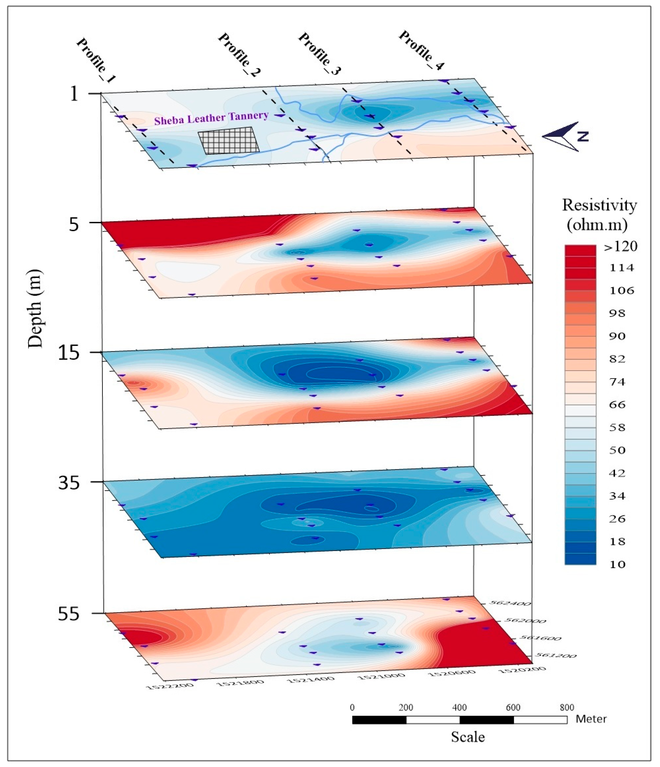
5.1.2. The 3D Resistivity Slice Model

The study area was further analyzed using a 3D resistivity slice model to gain a comprehensive understanding of the resistivity distribution at different depths. In general, 3D models give very important information about the aquifer nature and the structure of the associated subsurface formations [75]. The model provides valuable insights into the groundwater conditions and potential contamination in the vicinity of the tannery area.

The resistivity of the slice map (Figure 5) at a depth of 5 m is generally high, except for the central region, particularly near Profile 3. This suggests that the groundwater in the central zone may have different characteristics compared to the surrounding areas. The slice map at a depth of 15 m reveals low resistivity in the central zone of the survey area, primarily observed in profiles 2 and 3. This indicates the presence of groundwater with potentially higher concentrations of pollutants. The slice map at a depth of 35 m consistently displays very low resistivity values throughout the survey area. This suggests the possible presence of contaminants. It aligns with findings from the geoelectric profiles, indicating a clear correlation between low resistivity and groundwater pollution. The resistivity distribution depends on the pollution level; low resistivity is shown in highly polluted places whereas relatively high resistivity in unpolluted places [76,77]. The bottom slice map at a 55 m depth exhibits a relatively high resistivity distribution overall, with a low resistivity response in the central zone. This pattern further supports the presence of contaminated groundwater in the central area, likely to originate from the tannery area waste. The observed decreasing trend in resistivity downstream of the Tannery area, as well as the depth-wise decrease to 35 m strongly suggests the presence of groundwater pollution. The areas with reduced electrical resistivity, as identified in both the 3D model and the individual profiles (Profile 2 and Profile 3), are highly indicative of layers carrying water contaminated by the tannery area waste. The 3D resistivity slice model provides valuable insights into the spatial distribution of resistivity at different depths, helping us understand the extent and potential impact of groundwater pollution in the study area.

5.2. Hydrochemical Characterization

5.2.1. Physicochemical Characteristics of the Water Samples

The physicochemical analysis of 9 surface water and 23 groundwater samples was performed. A summary of the descriptive statistics for the major ions is presented in

Table 2. Descriptive statistics for the cations (mg/L), anions (mg/L), Na⁺(%), and SAR.

Parameters	Min	Max	Mean	Median	Mode	STD
Ca2+	51	255	158	162	142	51.4
Mg2+	7	64	31.5	29	32	14.8
Na+	5.8	134.1	44.8	30.8	14.8	34.4
K+	2.03	16.4	5.4	4.81	4.81	3.2
HCO3−	54.9	652.7	296.8	304.9	396.5	114.6
SO42−	98.6	702.6	293.4	295.1	435.6	130.9
Cl−	1.52	172.5	42.2	22.6	12.6	44.73
NO3−	0.52	81.9	18.1	11.2	38.6	17.5
Cr6+	0	0.82	0.07	0.01	0.01	0.14
Cu2+	0.01	1.53	0.64	0.61	0.61	0.27
Fe2+	0.21	0.97	0.57	0.56	0.61	0.19
Mn2+	0	0.09	0.01	0.01	0	0.02
Na+(%)	4.09	35.15	16.11	12.87	----	8.17
SAR	0.12	2.4	0.86	0.58	----	0.59

, and the results of the complete analysis are shown in

Table 3. Results of physicochemical parameters of 32 water samples. Shallow wells (S), Hand-dug wells (H), River water (R), and Spring (SP). All are reported in mg/L, except for EC, which is in µS/cm (25 °C). The pH, WQI, and SAR are dimensionless.

ID	pH	TDS	EC	Na+	K+	Ca2+	Mg2+	HCO3−	SO42−	Cl−	NO3−	Cr6+	Cu2+	Fe2+	Mn2+	WQI	SAR
S1	7.41	836	1306	14.80	2.74	186	7	365.9	256.4	1.52	0.86	0.01	0.61	0.61	0.00	80.14	0.28
S2	6.91	731	1142	39.14	3.93	110	32	229.40	291.80	18.70	4.81	0.02	0.58	0.73	0.00	88.74	0.84
S3	7.14	638	998	25.90	4.81	66	56	369.79	98.60	12.60	3.61	0.01	0.92	0.43	0.00	71.21	0.56
S4	6.84	495	773	14.10	3.72	62	31	239.20	131.80	8.30	4.16	0.02	0.73	0.21	0.00	60.54	0.36
S5	7.06	875	1367	14.80	2.84	128	15	396.50	306.40	7.90	2.18	0.00	0.81	0.61	0.00	76.89	0.32
S6	7.24	951	1487	17.24	5.77	207	30	317.20	356.80	11.50	5.14	0.01	0.56	0.38	0.00	96.65	0.29
S7	7.48	820	1281	29.87	4.39	142	51	237.89	291.40	46.70	15.60	0.03	0.87	0.51	0.03	94.64	0.54
S8	6.71	1145	1789	33.60	11.63	204	51	436.20	325.80	47.80	33.70	0.06	0.73	0.72	0.04	167.45	0.54
H1	5.02	1255	1960	37.50	16.44	255	36	652.70	214.80	28.90	12.80	0.01	0.88	0.38	0.01	157.81	0.58
H2	6.81	801	1251	25.40	2.03	170	14	335.50	226.90	17.30	9.64	0.00	0.31	0.52	0.00	78.73	0.5
H3	7.62	1186	1853	89.50	5.13	220	33	173.20	505.20	146.70	12.81	0.03	0.72	0.28	0.03	128.07	1.48
H4	6.25	1255	1960	134.10	8.51	189	28	374.50	412.60	71.80	35.90	0.02	0.81	0.71	0.01	175.74	2.4
H5	8.42	348	543	20.90	2.21	51	12	121.90	121.80	12.60	5.21	0.01	0.28	0.73	0.00	61.35	0.68
H6	7.02	438	684	28.70	4.41	76	10	168.10	126.40	15.80	8.11	0.00	0.32	0.81	0.00	67.01	0.81
H7	7.69	1195	1867	55.30	15.35	231	32	54.90	702.90	71.90	31.60	0.02	0.41	0.52	0.00	224.61	0.9
H8	7.43	772	1206	64.50	6.91	107	21	254.30	261.80	33.70	20.80	0.82	0.49	0.81	0.01	122.63	1.48
H9	8.05	986	1540	107.50	4.84	142	21	304.90	322.40	51.60	31.70	0.03	0.37	0.51	0.03	139.04	2.22
H10	6.70	1311	2048	127.24	4.40	206	57	289.10	435.60	151.60	38.60	0.14	1.14	0.89	0.07	181.7	2.01
H11	7.22	914	1428	39.84	5.19	131	41	457.49	192.70	39.20	6.53	0.04	0.73	0.63	0.06	87.14	0.77
H12	6.69	1394	2178	108.53	5.39	246	64	122.00	591.50	172.50	81.90	0.25	1.53	0.95	0.09	269.26	1.58
H13	7.28	930	1453	32.11	3.64	165	50	317.19	302.80	33.40	24.50	0.05	0.69	0.64	0.02	112.39	0.56
H14	7.54	1024	1600	102.44	3.24	125	39	134.20	435.60	131.60	51.60	0.12	0.96	0.97	0.03	167.21	2.04
R1	7.54	655	1023	28.30	5.62	128	22	237.90	201.60	21.60	9.72	0.00	0.52	0.61	0.00	84.43	0.6
R2	6.72	878	1371	31.40	5.86	175	26	304.90	308.80	16.80	8.72	0.02	0.48	0.36	0.01	98.25	0.58
R3	6.81	926	1446	27.90	5.55	203	24	353.80	291.60	14.40	5.15	0.01	0.63	0.28	0.00	89.18	0.49
R4	6.52	757	1182	28.20	5.32	142	25	305.00	208.10	21.70	21.70	0.00	0.48	0.43	0.00	100.95	0.57
R5	7.10	788	1231	30.30	5.12	159	23	323.30	203.60	21.50	21.50	0.01	0.54	0.41	0.00	95.83	0.59
R6	6.54	815	1273	28.80	4.81	144	19	396.50	203.60	13.60	4.98	0.01	0.01	0.41	0.00	66.56	0.59
R7	8.02	636	993	5.81	4.34	137	20	243.90	220.60	2.86	0.52	0.01	0.61	0.69	0.02	78.71	0.12
R8	6.89	959	1498	27.51	2.05	186	46	341.60	293.50	39.60	21.80	0.03	0.54	0.63	0.08	102.71	0.46
R9	7.54	918	1434	26.89	3.75	174	50	268.40	314.90	41.50	38.60	0.01	0.38	0.51	0.02	126.14	0.46
SP	7.08	876	1368	35.50	2.99	180	24	372.10	231.70	23.60	5.27	0.00	0.61	0.35	0.01	80.71	0.65

. In the first group of samples, i.e., shallow wells, the pH ranges from 6.52 to 8.02, and TDS ranges from 495 to 1145 mg/L. The river waters show a narrow range of pH (6.71 to 7.48), and the TDS ranges from 636 to 959 mg/L. The hand-dug wells comparatively indicate a wider range of pH and TDS. Remarkably higher values of TDS were observed in hand-dug wells H7, H10, H12, and H14. The descriptive statistics of the hydrochemical variables for the major cations and anions are shown in Table 2. The major cations (Ca²⁺, Mg²⁺, Na⁺, K⁺) and anions (HCO₃⁻, SO₄²⁻, Cl⁻ and NO₃⁻) show high variability evident from the standard deviations. Such high standard deviations indicate that the groundwater characteristics are affected by complex factors [78]. In our study area, the primary factors influencing ion concentration variability are the geology and hydrogeological processes, both of which are classified as natural factors. The weathering and dissolution of calcite and dolomite, common in our study area, contribute to significant amounts of calcium, magnesium, and bicarbonate ions. In addition to the calcium resulting from the dissolution of calcite and dolomite, gypsum dissolution also contributes additional calcium and sulfate ions. Alongside the variability due to natural factors, anthropogenic impacts also play a significant role in altering the water chemistry. Notably, irregular loads of sodium, chromium, chloride, and sulfate are sourced from the tannery area. Additionally, chloride, sulfate, and nitrate can result from sewage, agricultural activities, and runoff from Wikro City.

5.2.2. Hydrogeochemical Processes Interpretation

Figure 6A illustrates a cross plot of Ca²⁺ versus HCO₃⁻ for the water samples, including shallow wells, hand-dug wells, springs, and river water. The processes of calcite dissolution that release calcium and bicarbonate into the groundwater can be described as follows (Equations (6) and (7)):

CaCO₃ + CO₂ + H₂O → Ca²⁺ + 2HCO₃⁻

(6)

CaMg (CO₃)₂ + 2CO₂ + 2H₂O → Ca²⁺ + Mg²⁺ + 4HCO₃⁻

(7)

The possible primary source for Ca²⁺ is calcite mineral dissolution, as the main aquifer of the study area is fractured limestone [25]. Except for two shallow wells and one hand-dug well, all water samples fall above the 1:1 line plot (Figure 6A), indicating that calcite dissolution is the main process contributing to Ca²⁺ and HCO₃⁻. However, in some hand-dug well samples (H3, H7, H10, H12), high Ca²⁺ levels are observed with low HCO₃⁻, suggesting that the source of Ca²⁺ in these samples is not solely from the dissolution of calcite minerals. The gypsum layer is found sandwiched between the shale–limestone intercalation rock unit [25]. Therefore, gypsum can be an additional source of Ca²⁺. The process of gypsum dissolution, which releases Ca²⁺ and SO₄^2- into the groundwater, is represented by Equation (8):

CaSO₄·2H₂O → Ca²⁺ + SO₄²⁻ + 2H₂O

(8)

In Figure 6B, we plot the relationship between Ca²⁺ and SO₄²⁻. The results indicate that all water samples are situated above the 1:1 line, which strongly suggests the presence of an additional source of Ca²⁺ in the solution, in addition to gypsum dissolution. For the further evaluation of Ca²⁺ enrichment, we plot the Ca²⁺ + Mg²⁺ versus HCO₃⁻ + SO₄²⁻ ratio (Figure 6C). The plot reveals that four hand-dug wells, two shallow wells, and one river water sample fall on the 1:1 line, indicating the same source which is the dissolution of calcite, dolomite, and gypsum. The remaining samples fall above the 1:1 line, suggesting the presence of another source, namely the tannery area effluents. Additionally, Na⁺ versus Cl^- is plotted (Figure 6D). Two hand-dug wells (H3 and H12), two shallow wells (S7 and S8), and three river waters (R7, R8, R9), all collected from the downstream side of the tannery area, align on the 1:1 line, representing the tannery area effluents as the common source. Since no halite strata occur in the subsoil of the study area, it could rather be the tannery area effluents that are the source as the tannery area uses various salts during leather processing [22]. Five hand-dug well samples (H3, H7, H10, H12, and H14) collected downstream and near the tannery area show high Cl^- concentrations compared to the other samples. These results are also supported by the Piper diagram (Figure 7), as all of these samples showed high chloride concentrations. The Cl⁻ versus NO₃⁻ graph (Figure 6E) reveals the possible sources of Cl⁻ enrichment, as both ions are usually found in domestic sewage [79]. The higher concentration of Cl⁻ suggests yet another source besides domestic sewage, which is the tannery area effluents. NO₃⁻ versus SO₄²⁻ was also plotted (Figure 6F) and indicates that these two anions (NO₃⁻ and SO₄²⁻) do not have the same source. This implies that the SO₄²⁻ enrichment in this area was not due to the fertilizers. A previous research work [63] suggests fertilizer as a source of SO₄²⁻, but in this case, it is rather due to the tannery area effluents. Therefore, it can be deduced that the tannery area effluents had a prevailing and negative influence on hydrochemistry in the downstream area (H3, H4, H7, H10, H12, and H14).

5.2.3. Correlation Among Selected Parameters

Pearson’s correlation matrix using 15 parameters was performed to evaluate the relationship and the influence of each parameter over the other (

Table 4. Pearson’s correlation matrix of 15 selected parameters; values above 0.75 are highlighted in bold.

	pH	TDS	EC	Na+	K+	Ca2+	Mg2+	Fe2+	Cu2+	Cr6+	Mn2+	Cl−	HCO3−	SO42−	NO3−
pH	1
TDS	−0.1	1
EC	−0.03	0.96	1
Na+	0.04	0.30	0.28	1
K+	−0.1	−0.05	−0.05	0.15	1
Ca2+	−0.22	0.09	0.07	0.32	0.49	1
Mg2+	0.01	−0.05	−0.11	0.32	0.16	0.30	1
Fe2+	0.20	−0.03	−0.08	0.53	−0.11	−0.1	0.17	1
Cu2+	−0.02	−0.09	−0.14	0.46	0.10	0.31	0.66	0.27	1
Cr6+	−0.08	−0.11	−0.12	0.17	0.57	0.44	0.27	0.02	0.41	1
Mn2+	−0.06	0.15	0.05	0.41	−0.06	0.37	0.70	0.42	0.60	0.21	1
Cl−	0.10	0.25	0.21	0.83	0.11	0.44	0.56	0.43	0.62	0.22	0.66	1
HCO3−	−0.25	−0.02	0.01	−0.22	0.24	0.23	0.01	−0.3	0.01	0.43	−0.05	−0.38	1
SO42−	0.02	0.13	0.10	0.61	0.35	0.67	0.36	0.26	0.38	0.08	0.39	0.74	−0.4	1
NO3−	−0.06	0.01	−0.04	0.70	0.18	0.41	0.58	0.57	0.52	0.22	0.59	0.78	−0.32	0.66	1

). Based on the correlation coefficients (r), the significance was classified into three groups: high (r > 0.75), medium (0.5 < r < 0.75), and low (r < 0.5), regardless of whether the correlation was positive or negative. As expected, TDS, EC, Na⁺, Cl⁻, NO₃⁻, and SO₄²⁻ were related due to their high-to-medium correlation. The TDS has a high correlation with EC (0.96). The high Na⁺ correlation with Cl⁻ (0.83) is due to the NaCl used by the tannery area in processing the hides. Na⁺ and Cl⁻ indicate a positive, although, in most cases, a low correlation with all parameters in the entire matrix, except with bicarbonate, referring to the tannery area effluents. Moreover, Na⁺ has a medium correlation with NO₃⁻ (0.70), which indicates the presence of other common anthropogenic pollution sources for both ions (Na⁺ and NO₃⁻), which could be from agriculture or municipal sewage. These two possible anthropogenic pollution sources are further confirmed by the high correlation of NO₃⁻ with Cl⁻ (0.78). Na⁺ has a lower correlation with Ca²⁺ (0.32), and a correlation between Na⁺ and Ca²⁺ suggests the presence of different kinds of hydrochemical influencing factors [80]. The Na⁺ has a medium correlation with SO₄²⁻ (0.61) and SO₄²⁻ with Cl⁻ (0.74), which could be from salts, including sodium sulfate and sodium hydrogen sulfide, used by the plant [21]. SO₄²⁻ has a medium correlation with Ca²⁺ (0.67), which could be due to the tannery area effluents’ and/or the presence of gypsum in the study area. The hydrochemical spatial distribution (in Section 5.2.7) also shows that the tannery area contribution for the SO₄²⁻ increments is substantial as the concentration is highly enriched downstream of the tannery area. Most of the parameters show a low correlation with HCO₃⁻. The NO₃⁻ is highly correlated with Cl⁻ (0.78) and moderately correlated with Mn²⁺ (0.59), Mg²⁺ (0.58), Fe²⁺ (0.57), and Cu²⁺ (0.52). These medium-to-high correlations are in line with the fact that NO₃⁻ collectively reflects the contamination of water resources from anthropogenic activities.

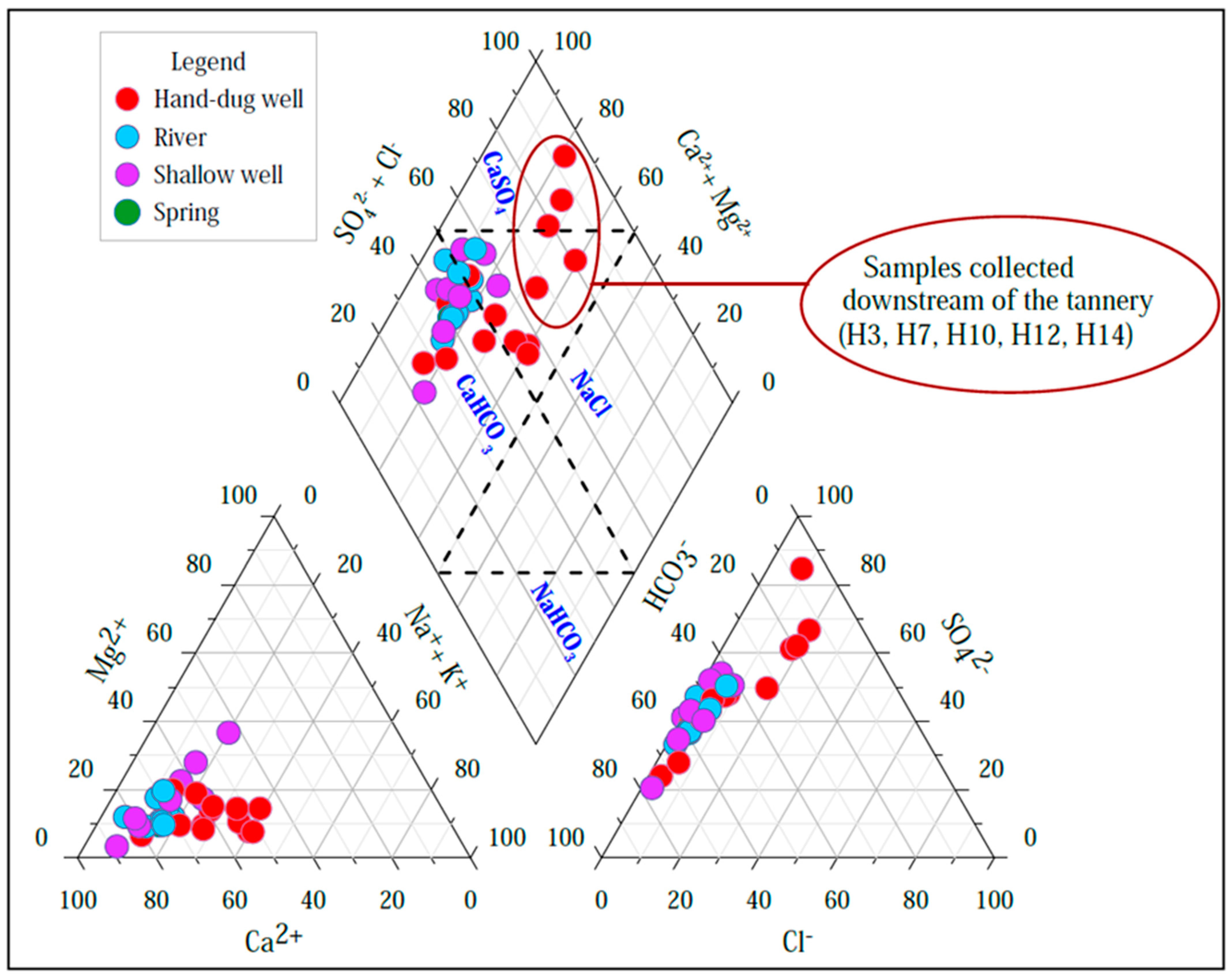
5.2.4. Hydrochemical Facies

The tendency of the order of major cations and anions in the water samples of the current investigation, in equivalent concentrations, is shown in the Piper diagram (Figure 7). The groundwater-type classification with a Piper diagram is widely used and applied by various researchers [80,81,82]. The effect of the complex hydrochemical interactions between the rocks and the groundwater and the spatial as well as temporal evolution is reflected in the hydrochemical facies. Hydrochemical facies reveal changes in the water type as a result of water–rock interactions, most intensively in shallow-depth groundwater resources [83]. Accordingly, from the diagram (Figure 7), the recognized groundwater types are CaHCO₃, Ca/MgHCO₃, Ca/MgSO₄, and CaSO₄. All possible anthropogenic sources, including those causing an increase in TDS and SO₄²⁻ in groundwater resources, are global groundwater quality management issues [84,85,86]. The release of SO₄²⁻ into groundwater is the main cause for changing the shallow fresh groundwater chemistry in the investigated area and shifting the samples up in the Piper diagram.

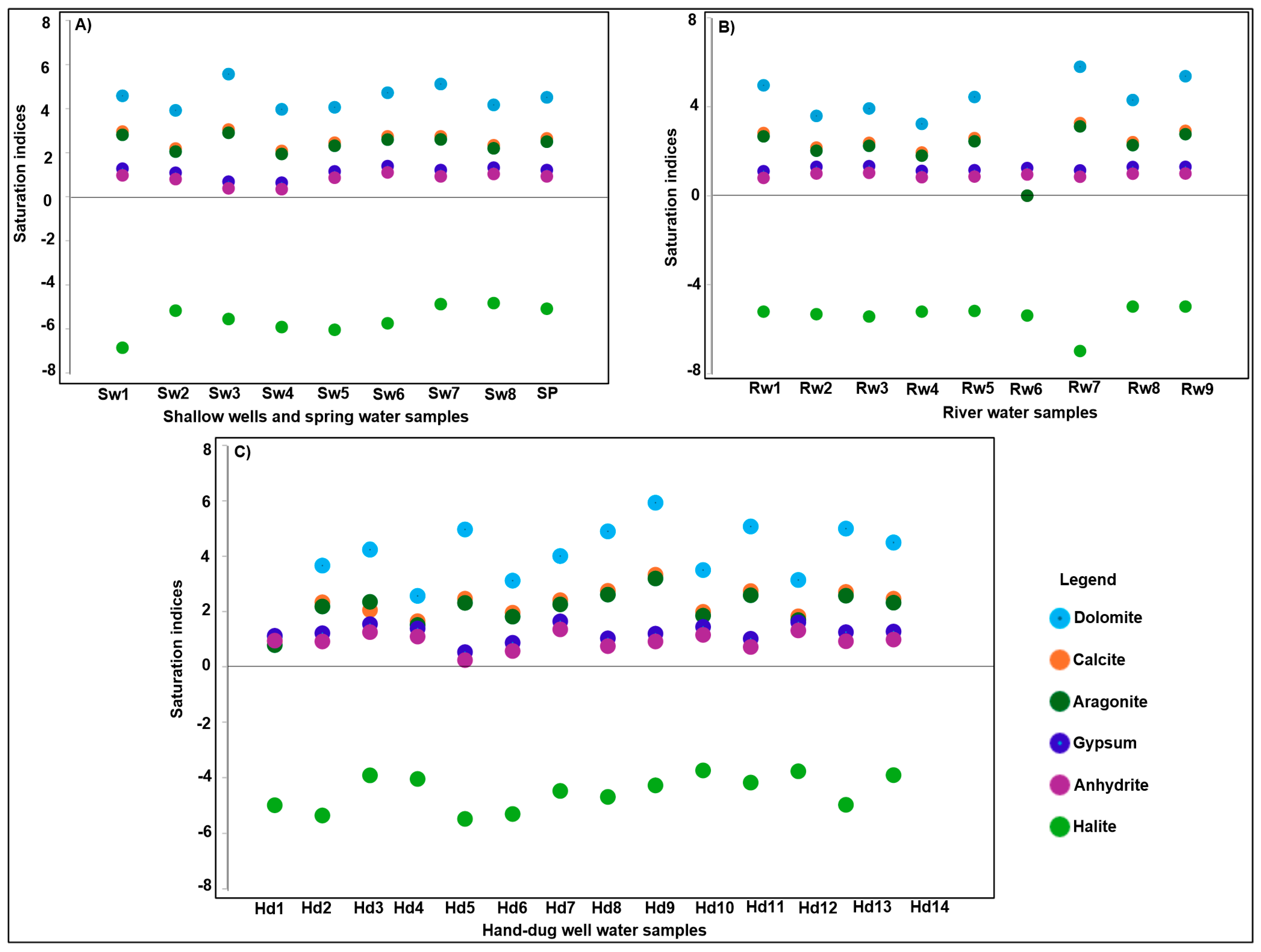
5.2.5. Saturation Indices (SI)

The saturation state, i.e., the chemical equilibrium of the groundwater, has been examined for each collected water sample. Except for halite, all samples are supersaturated concerning the anhydrite, aragonite, calcite, dolomite, and gypsum minerals (Figure 8). The calculated SI values, in ascending order, are halite, anhydrite, gypsum, aragonite, calcite, and dolomite. As was observed during the geological field mapping, a gypsum unit is exposed a few km east of the tannery area (Figure 2). Also, the unpolluted water has high sulfate due to the gypsum that is locally present in the aquifer, which is the reason for the positive SI for gypsum and anhydrite. In addition, the anthropogenically sourced SO₄²⁻, which abundantly shows its effect downstream of the tannery area, contributes to the supersaturation. As explained above, the groundwater-bearing geological formations of the Wikro area and its surroundings are characterized by fractured limestone and shale–limestone intercalations together with thin sandwiched gypsum layers [25,87]. Therefore, water–rock interactions in such a kind of environment will increase the ionic concentration of the groundwater. Moreover, calcium, magnesium, sodium, and sulfate concentrations are high in samples collected from nearby, and downstream the tannery area due to the tannery area effluents experiences infiltration because the Sheba tannery area used chrome salt, sodium sulfide, sodium hydrogen sulfide, calcium hydroxide, magnesium hydroxide, and other salts [22]. The combined impact of the lithological types found in the study area and the tannery area effluents will result in a high concentration of ions in the groundwater.

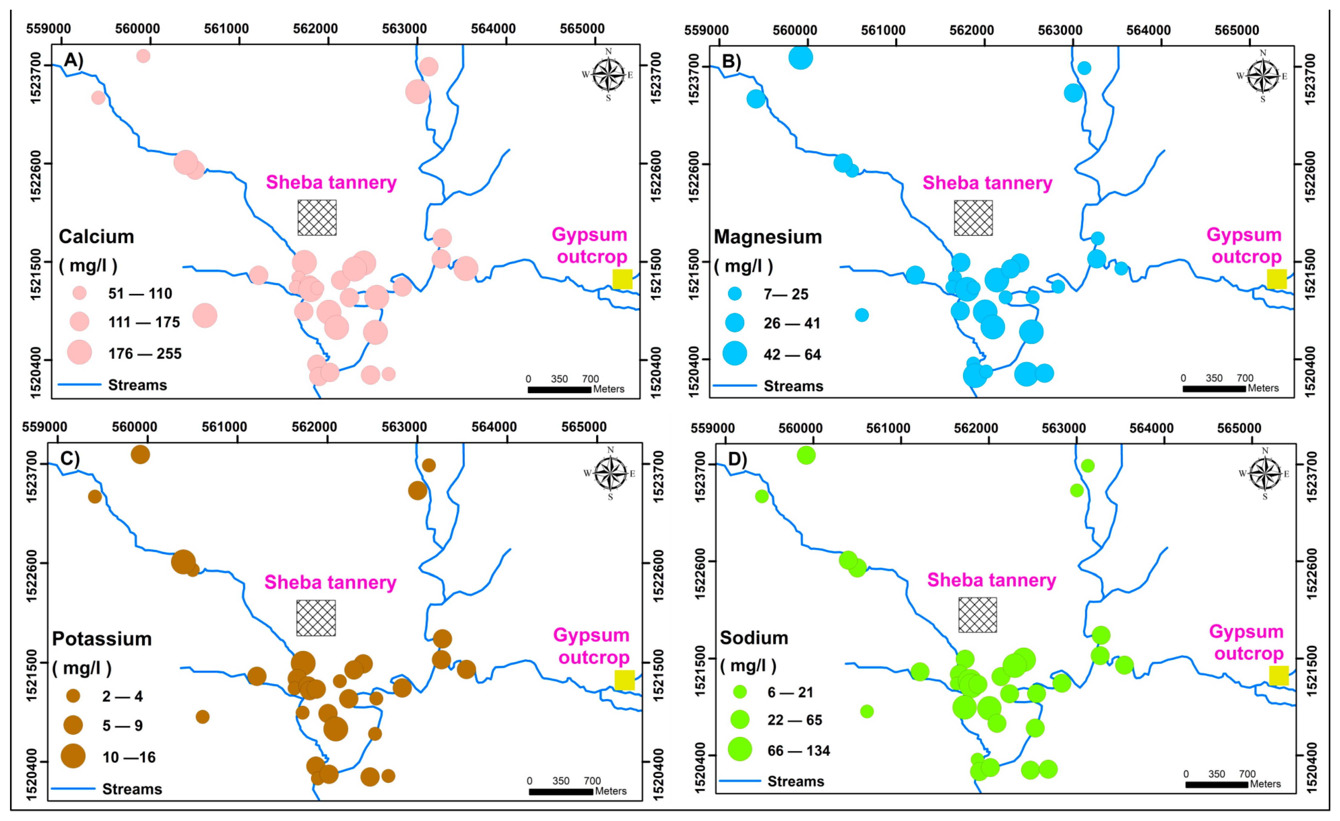
5.2.6. Evaluation of Pollution Status Using Major Cations Concentration

The local hydrochemical processes of the study area and the pollution status were evaluated by integrating geophysical and hydrochemical methods. Spatial concentration distributions of the major cations were mapped (Figure 9), and the possible hydrochemical variations due to the water–rock interaction and anthropogenic factors were determined. The pollution status and pollutant sources were commonly evaluated, focusing on residential area distribution, sewage discharges, and industrial activities [88]. The Na⁺ shows a significantly higher concentration, particularly at H4, H10, H12, and H14 downstream of the tannery area, which is due to the effluents as different sodium-based salts were used in the tannery area [22]. The possibility for a naturally high Na⁺ concentration in groundwater resources can be found when sodic plagioclase minerals, which are mostly found in volcanic rocks [89], are present, but that was not the case in our study area. Therefore, these two reasons, i.e., lower concentration at the upstream side and no volcanic rocks in the area, imply that the Na⁺ is most probably sourced from the tannery area.

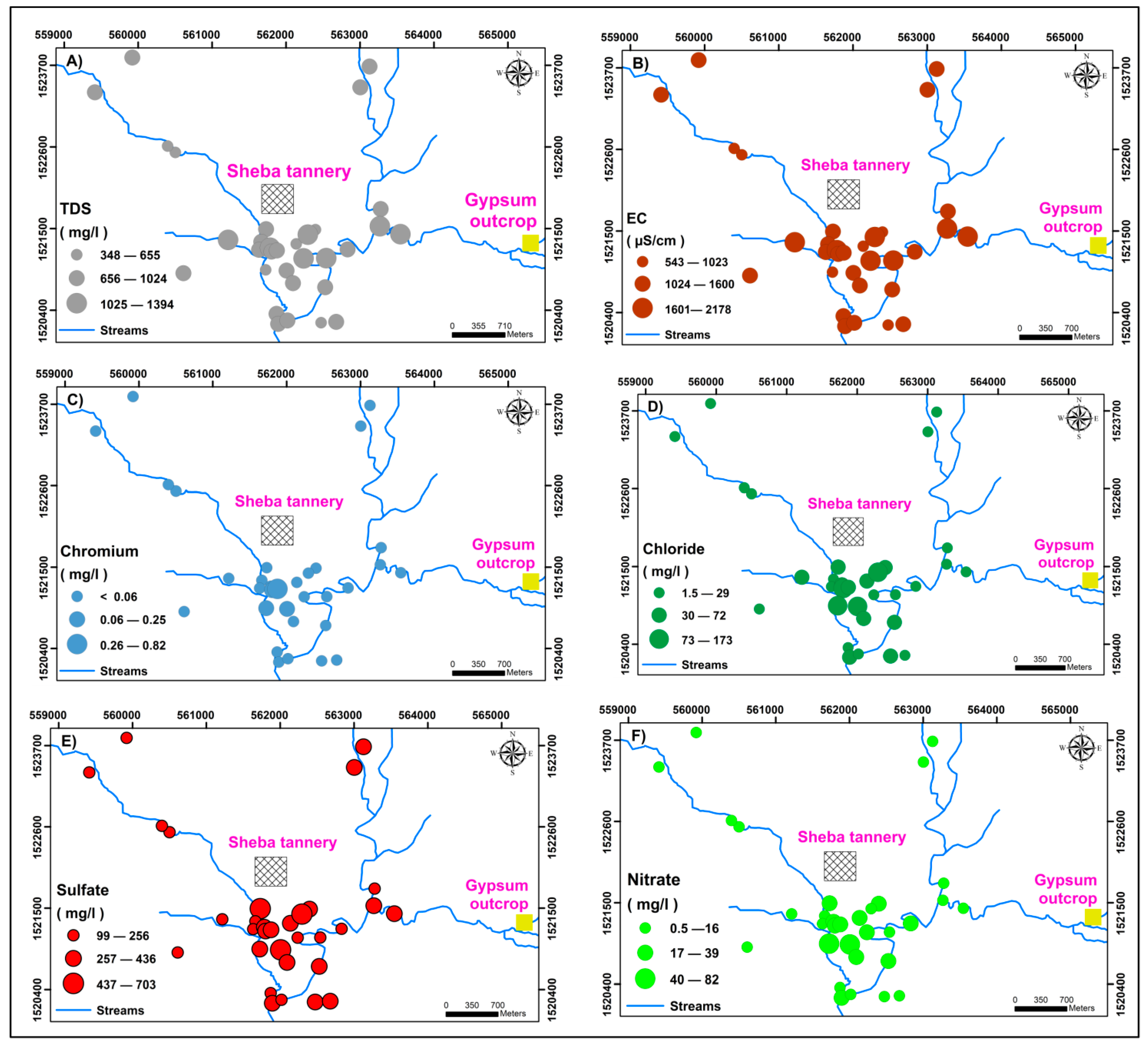
5.2.7. Evaluation of Pollution Status Using EC, TDS, Anions, and Selected Heavy Metals

The concentrations observed for the anions, particularly SO₄²⁻, Cl⁻, and NO₃⁻, downstream of the tannery area are higher compared to their concentrations upstream. This could serve as evidence that the pollution impact is higher downstream. The SO₄²⁻ concentration varies from 99 mg/L to 703 mg/L. The significantly higher concentrations were dominantly found in the hand-dug wells, and this particular ion was the main factor changing the hydrochemistry in the study area, as is also shown in the Piper diagram (Figure 7). Similarly, acids, alkalis, chromium salts, and sulfides used in leather tanneries for transforming raw skin into commercial goods are abundantly found in wastewater effluents [1]. Therefore, the sulfides and various salts used in the tannery area, which are detected in the effluents of the wastewater [22], could be the main sources of Cr⁶⁺, Cl⁻, and SO₄²⁻ concentration increases in the groundwater to the level of pollution in the study area (Figure 10C–E). The TDS and EC are also higher for samples collected downstream (Figure 10A,B). The main factors are SO₄²⁻, NO₃⁻, and Cl⁻; this is in line with the results presented in the correlation matrix (Table 4). The correlation matrix shows a high correlation coefficient between NO₃⁻ and Cl⁻ (r = 0.78) and a medium correlation between SO₄²⁻ and Cl⁻ (0.74). An increase in concentrations towards the downstream direction is also noted for NO₃⁻ (Figure 10F), though it was not highly correlated with the TDS and EC. The sources could be fertilizers applied with irrigation in the area, as the agricultural activities are more intense in the flat areas downstream compared to upstream. The agricultural activity in different parts of the developing country uses excess water and fertilizer to meet the increasing food demand [90]. Overall, the results of these different parameters show that the downstream areas of the tannery area are comparatively more polluted than those upstream. The heavy metals manganese, iron, and copper show maximum concentrations of 0.08 mg/L, 0.89 mg/L, and 0.96 mg/L, respectively. These elements can impact the ecological environment and animal and human health [91,92,93,94] when in very high concentrations.

5.3. Water Quality Index (WQI)

The WQI has been applied by several researchers [59,60,64,95]. Considering the parameters and weights listed in Table 1 (see Section 4. Materials and Methods), the results generally showed that 56.3% of the water samples fell under good, 37.5% under poor, and 6.2% under very poor class for drinking.

Specifically, the calculated WQI scores for the shallow wells ranged from 60.5 to 167.4, with 96.4 as an average value. Seven out of eight shallow wells (87.5%) were classified as good; however, one of them (S8), i.e., 1.25%, was classed as poor. S7 and S8, which have a WQI score of 94.6 and 167.4, respectively, are located downstream of the tannery area. For the hand-dug wells, the WQI had a range from 61.4 to 269.3 and a mean of 143.9. Out of the 15 samples including the spring water, 5 (33.3%) were classified as good, 8 (i.e., 53.3%) were poor, and 2 (i.e., 13%) were very poor. The very poor class corresponded to hand-dug wells H7 and H12. H7 is close to the tannery area, and H12 is downstream, close to a confluence of three streams that drain the tannery area and its surroundings. The river water samples showed a WQI range from 66.6 to 126.1 and a mean of 94.13. Six out of nine (67%) samples indicated a good class, whereas 33% were poor. In all three sample varieties, the highest values of WQI were recorded for samples in downstream regions of the tannery area, which could be due to the high TDS load from the tannery area effluents. The calculated WQI showed that 2 samples were in the very poor class, 12 samples were poor, and the remaining 18 samples fell under the good class. Therefore, around 44% of the water in this study area needs proper quality treatment to be used for drinking purposes. Moreover, it is worth noting that bacteriological analysis was not conducted during this study and that the reported viability of the water sources for drinking is not conclusive.

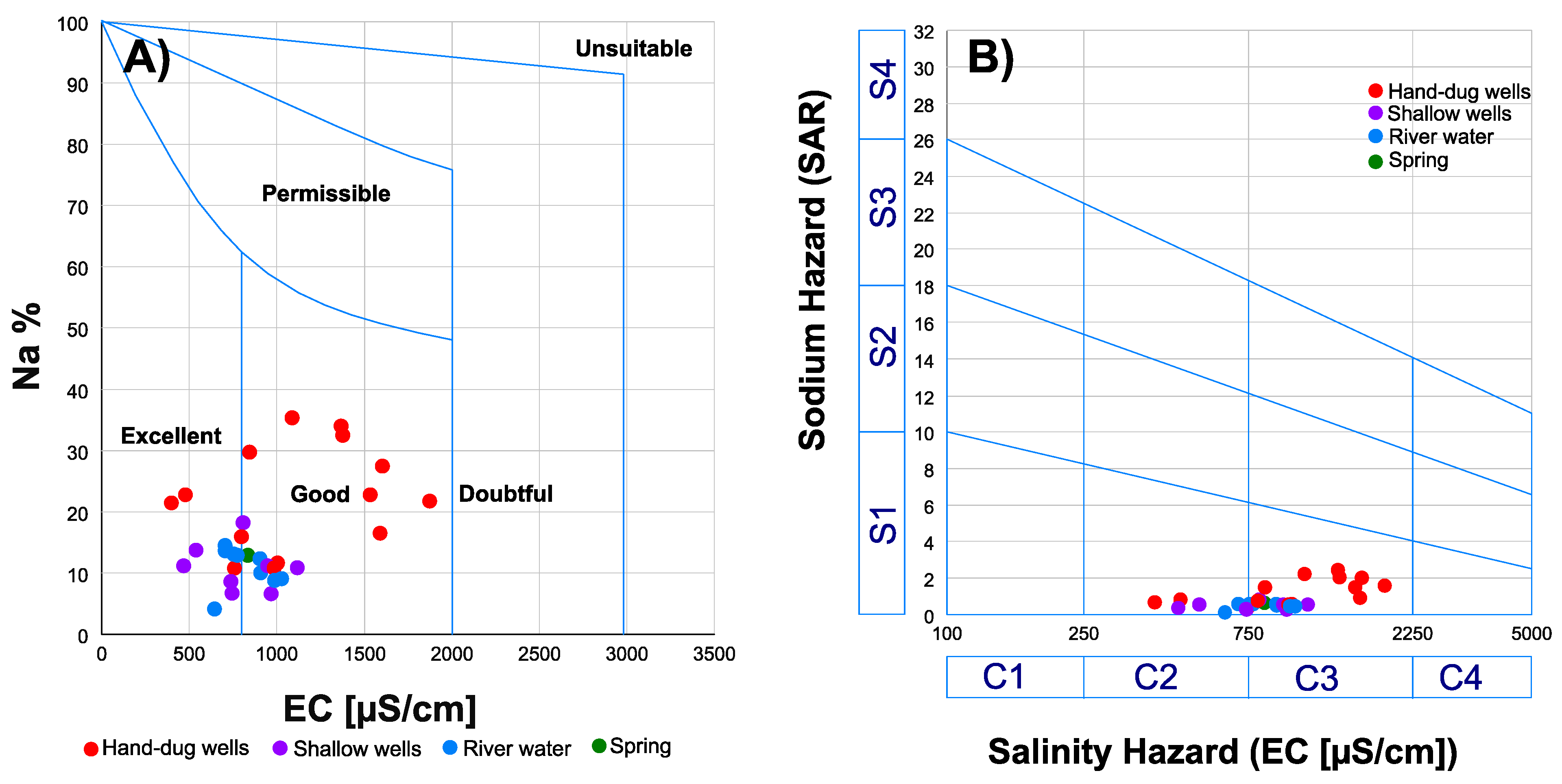
5.4. Quality Suitability Assessment for Irrigation

Two irrigation indices (Figure 11A,B) of the Na⁺ adsorption ratio (SAR) and the Na⁺ percentage (Na⁺%), were evaluated to determine the viability of the water for irrigation. The values for SAR and Na⁺%) ranged from 0.12 to 2.4, with a mean of 0.86, and from 4.09 to 35.15, with a mean of 16.11, respectively. According to [96], water with a SAR value >10 is harmful. In light of this, all of the samples show SAR values within the permissible limit. Moreover, in the case of the Na⁺%, all of the samples fell in the excellent and good zones, according to the [97] classification of irrigation water; 12.5% of the samples fell in the “excellent” class, and 87.5% fell into the “good” category. Therefore, even though crop-specific studies should be further conducted, the groundwater in this area is generally suitable for irrigation.

6. Conclusions

The VES survey mainly showed three to four geological layers and fracture zones. The findings indicate the presence of very low resistivity zones, which are interpreted to be polluted groundwater zones, probably due to effluents from the tannery area. The four constructed profiles clearly show the presence of contaminated zones as one crosses from Profile 1 to Profile 4, which are aligned north to south, locally in the direction of surface and groundwater flow.

The hydrochemical analysis results also show that the concentration of ions, especially SO₄²⁻ and Cl⁻, Na⁺, and heavy metals, tend to be higher in the shallow groundwater samples collected from Profile 2 and Profile 3 in the surrounding areas. Therefore, these ions and heavy metal concentration results are in line with the geophysical survey results. The prominent hydrochemical facies are CaHCO₃, Ca/MgHCO₃, Ca/MgSO₄, and CaSO₄. The quality status, according to the WQI, falls under the classes of good, poor, and very poor for drinking but is suitable for irrigation, except for three hand-dug well samples (H4, H10, H14) that show high SAR values. For a deeper understanding, the temporal variability of the water quality parameters should be studied further. The findings in this study serve as a benchmark for future investigations in the study area. The integrated method of geophysical and hydrochemical studies used in this work to investigate shallow groundwater quality and determine water quality indices offers numerous advantages globally, particularly in developing countries that usually face issues related to water scarcity, quality, and management.

Finally, since this leather tannery area is located upstream of a major water supply dam, we recommend further detailed investigation of the contamination and status monitoring of this groundwater resource, such as by drilling test wells and taking depth-specific sampling. This can allow for a comprehensive understanding of the groundwater quality. It is essential to understand the depth and distribution of contaminants to design effective remediation strategies. Moreover, it may help to determine the most suitable depth for installing remediation systems, such as wells or barriers, to target and contain or treat contaminated zones. We also recommend that, during the rehabilitation of the Sheba Leather Tannery area, green chemistry is integrated where the tannery area effluents are minimized, contained, and treated to protect the environment and water resources.

References

1. Lofrano, G.; Meriç, S.; Zengin, G.E.; Orhon, D. Chemical and biological treatment technologies for leather tannery area chemicals and wastewaters: A review. Sci. Total Environ. 2013, 461, 265–281. [Google Scholar] [CrossRef]
2. Magesh, N.S.; Chandrasekar, N.; Elango, L. Trace element concentrations in the groundwater of the Tamiraparani river basin, South India: Insights from human health risk and multivariate statistical techniques. Chemosphere 2017, 185, 468–479. [Google Scholar] [CrossRef] [PubMed]
3. Vignati DA, L.; Ferrari, B.J.; Roulier, J.L.; Coquery, M.; Szalinska, E.; Bobrowski, A.; Czaplicka, A.; Kownacki, A.; Dominik, J. Chromium bioavailability in aquatic systems impacted by tannery area wastewaters. Part 1: Understanding chromium accumulation by indigenous chironomids. Sci. Total Environ. 2019, 653, 401–408. [Google Scholar] [CrossRef]
4. Tadesse, G.L.; Guya, T.K.; Walabu, M. Impacts of tannery area effluent on environments and human health: A review article. Adv. Life Sci. Technol. 2017, 54, 58–67. [Google Scholar]
5. Hammons, A.S.; Huff, J.E.; Braunstein, H.M.; Drury, J.S.; Shriner, C.R.; Lewis, E.B.; Whitfield, B.L.; Towill, L.E. Reviews of the Environmental Effects of Pollutants: IV. Cadmium; Oak Ridge National Lab: Oak Ridge, TN, USA, 1978. [Google Scholar]
6. Schwingl, P.J.; Lunn, R.M.; Mehta, S.S. A tiered approach to prioritizing registered pesticides for potential cancer hazard evaluations: Implications for decision making. Environ. Health 2021, 20, 13. [Google Scholar] [CrossRef] [PubMed]
7. McCance, W.; Jones, O.; Cendón, D.; Edwards, M.; Surapaneni, A.; Chadalavada, S.; Currell, M. Decoupling wastewater impacts from hydrogeochemical trends in impacted groundwater resources. Sci. Total Environ. 2021, 774, 145781. [Google Scholar] [CrossRef]
8. Aristone, C.; Mehdi, H.; Hamilton, J.; Bowen, K.L.; Currie, W.J.; Kidd, K.A.; Balshine, S. Impacts of wastewater treatment plants on benthic macroinvertebrate communities in summer and winter. Sci. Total Environ. 2022, 820, 153224. [Google Scholar] [CrossRef] [PubMed]
9. López Arias, T.R.; Franco, D.; Medina, L.; Benítez, C.; Villagra, V.; McGahan, S.; Duré, G.M.; Kurita-Oyamada, H.G. Removal of Chromium (III) and reduction in toxicity in a primary tannery effluent using two floating macrophytes. Toxics 2024, 12, 152. [Google Scholar] [CrossRef] [PubMed]
10. Urbina-Suarez, N.A.; Ayala-González, D.D.; Rivera-Amaya, J.D.; Barajas-Solano, A.F.; Machuca-Martínez, F. Evaluation of the light/dark cycle and concentration of tannery wastewater in the production of biomass and metabolites of industrial interest from microalgae and cyanobacteria. Water 2022, 14, 346. [Google Scholar] [CrossRef]
11. Belay, A.A. Impacts of chromium from tannery effluent and evaluation of alternative treatment options. J. Environ. Prot. 2010, 1, 53. [Google Scholar] [CrossRef]
12. Fernandez, M.; Pereira, P.P.; Agostini, E.; González, P.S. Impact assessment of bioaugmented tannery effluent discharge on the microbiota of water bodies. Ecotoxicology 2020, 29, 973–986. [Google Scholar] [CrossRef] [PubMed]
13. Khan, M.A.; Costa, F.B.; Fenton, O.; Jordan, P.; Fennell, C.; Mellander, P.-E. Using a multi-dimensional approach for catchment scale herbicide pollution assessments. Sci. Total Environ. 2020, 747, 141232. [Google Scholar] [CrossRef]
14. Montalvão, M.F.; da Silva Castro, A.L.; de Lima Rodrigues, A.S.; de Oliveira Mendes, B.; Malafaia, G. Impacts of tannery effluent on development and morphological characters in a neotropical tadpole. Sci. Total Environ. 2018, 610, 1595–1606. [Google Scholar] [CrossRef]
15. Comber, S.; Gardner, M.; Ansell, L.; Ellor, B. Assessing the impact of wastewater treatment works effluent on downstream water quality. Sci. Total Environ. 2022, 845, 157284. [Google Scholar] [CrossRef] [PubMed]
16. De Sousa, A.; Wilhelm, C.M.; Da Silva, C.E.M.; Goldoni, A.; Rodrigues, M.A.S.; Da Silva, L.B. Treated tannery effluent and its impact on the receiving stream water: Physicochemical characterization and cytogenotoxic evaluation using the Allium cepa test. Protoplasma 2023, 260, 949–954. [Google Scholar] [CrossRef] [PubMed]
17. Mengistie, E.; Ambelu, A.; Van Gerven, T.; Smets, I. Impact of tannery effluent on the self-purification capacity and biodiversity level of a river. Bull. Environ. Contam. Toxicol. 2016, 96, 369–375. [Google Scholar] [CrossRef]
18. Ngobeni, P.V.; Mpofu, A.B.; Ranjan, A.; Welz, P.J. A Critical Review of Systems for Bioremediation of Tannery Effluent with a Focus on Nitrogenous and Sulfurous Species Removal and Resource Recovery. Processes 2024, 12, 1527. [Google Scholar] [CrossRef]
19. Younas, F.; Bibi, I.; Afzal, M.; Al-Misned, F.; Niazi, N.K.; Hussain, K.; Shahid, M.; Shakil, Q.; Ali, F.; Wang, H. Unveiling distribution, hydrogeochemical behavior and environmental risk of chromium in tannery wastewater. Water 2023, 15, 391. [Google Scholar] [CrossRef]
20. García-Valero, A.; Martínez-Martínez, S.; Faz, Á.; Terrero, M.A.; Muñoz, M.Á.; Gómez-López, M.D.; Acosta, J.A. Treatment of wastewater from the tannery industry in a constructed wetland planted with Phragmites australis. Agronomy 2020, 10, 176. [Google Scholar] [CrossRef]
21. Gebrekidan, A.; Weldegebriel, Y.; Hadera, A.; Van der Bruggen, B. Toxicological assessment of heavy metals accumulated in vegetables and fruits grown in Ginfel river near Sheba Tannery, Tigray, Northern Ethiopia. Ecotoxicol. Environ. Saf. 2013, 95, 171–178. [Google Scholar] [CrossRef] [PubMed]
22. Gebrekidan, A.; Gebresellasie, G.; Mulugeta, A. Environmental impacts of Sheba tannery (Ethiopia) effluents on the surrounding water bodies. Bull. Chem. Soc. Ethiop. 2009, 23. [Google Scholar] [CrossRef]
23. Amabye, T.G. Plant, soil and water pollution due to tannery effluent a case study from Sheb Tannery PLC, Wukro Tigray, Ethiopia. Science 2015, 3, 47–51. [Google Scholar]
24. Gebru, H.; Tadesse, N.; Konka, B. Impact of waste disposal from tannery on surface and groundwater, Sheba leather factory near Wurko, Tigray, Northern Ethiopia. Int. J. Earth Sci. Eng. 2012, 5, 665–672. [Google Scholar]
25. Gebreyohannes, T.; De Smedt, F.; Walraevens, K.; Gebresilassie, S.; Hussien, A.; Hagos, M.; Amare, K.; Deckers, J.; Gebrehiwot, K. Regional groundwater flow modeling of the Geba basin, northern Ethiopia. Hydrogeol. J. 2017, 25, 639. [Google Scholar] [CrossRef]
26. Alemayehu, T.; Leis, A.; Dietzel, M. Environmental isotope and hydrochemical characteristics of groundwater in central portion of Mekelle sedimentary outlier, northern Ethiopia. J. Afr. Earth Sci. 2020, 171, 103953. [Google Scholar] [CrossRef]
27. Abera, K.A.; Gebreyohannes, T.; Abrha, B.; Hagos, M.; Berhane, G.; Hussien, A.; Belay, A.S.; Van Camp, M.; Walraevens, K. Vulnerability mapping of groundwater resources of mekelle city and surroundings, tigray region, Ethiopia. Water 2022, 14, 2577. [Google Scholar] [CrossRef]
28. Damo, R.; Icka, P. Evaluation of Water Quality Index for Drinking Water. Pol. J. Environ. Stud. 2013, 22, 1045–1051. [Google Scholar]
29. Gupta, S.; Gupta, S.K. A critical review on water quality index tool: Genesis, evolution and future directions. Ecol. Inform. 2021, 63, 101299. [Google Scholar] [CrossRef]
30. Tyagi, S.; Sharma, B.; Singh, P.; Dobhal, R. Water quality assessment in terms of water quality index. Am. J. Water Resour. 2013, 1, 34–38. [Google Scholar] [CrossRef]
31. Khan, I.; Zakwan, M.; Pulikkal, A.K.; Lalthazula, R. Impact of unplanned urbanization on surface water quality of the twin cities of Telangana state, India. Mar. Pollut. Bull. 2022, 185, 114324. [Google Scholar] [CrossRef]
32. Arkin, Y.; Beyth, M.; Dow, D.; Levitte, D.; Temesgen Haile, T.H. Geological Map of Mekele Sheet Area ND 37-11, Tigre Province, 1: 250.000; Imperial Ethiopian Governement, Ministry of Mines, Geological Survey: Addis Ababa, Ethiopia, 1971. [Google Scholar]
33. Kazmin, V.; Shifferaw, A.; Balcha, T. The Ethiopian basement: Stratigraphy and possible manner of evolution. Geol. Rundsch. 1978, 67, 531–546. [Google Scholar] [CrossRef]
34. Tadesse, T. Structure across a possible intra-oceanic suture zone in the low-grade Pan-African rocks of northern Ethiopia. J. Afr. Earth Sci. 1996, 23, 375–381. [Google Scholar] [CrossRef]
35. Alene, M.; Ruffini, R.; Sacchi, R. Geochemistry and geotectonic setting of Neoproterozoic rocks from northern Ethiopia (Arabian-Nubian Shield). Gondwana Res. 2000, 3, 333–347. [Google Scholar] [CrossRef]
36. Kazmin, V. The geology of Ethiopia. Ethiop. Inst. Geol. Surv. Note 1972, 821012–821051. [Google Scholar]
37. Abdelsalam, M.G.; Stern, R.J. Sutures and shear zones in the Arabian-Nubian Shield. J. Afr. Earth Sci. 1996, 23, 289–310. [Google Scholar] [CrossRef]
38. Hagos, M.; Gebreyohannes, T.; Amare, K.; Hussien, A.; Berhane, G.; Walraevens, K.; Koeberl, C.; van Wyk de Vries, B.; Cavalazzi, B. Tectonic link between the Neoproterozoic dextral shear fabrics and Cenozoic extension structures of the Mekelle basin, Northern Ethiopia. Int. J. Earth Sci. 2020, 109, 1957–1974. [Google Scholar] [CrossRef]
39. Kaczor, D.; Sotysiak, M. Geophysical investigation in contamination hazard studies. Ecohydrol. Hydrobiol. 2006, 6, 223–232. [Google Scholar] [CrossRef]
40. Lopes, D.D.; Silva, S.M.; Fernandes, F.; Teixeira, R.S.; Celligoi, A.; Dall’Antônia, L.H. Geophysical technique and groundwater monitoring to detect leachate contamination in the surrounding area of a landfill–Londrina (PR–Brazil). J. Environ. Manag. 2012, 113, 481–487. [Google Scholar] [CrossRef]
41. Donohue, S.; McCarthy, V.; Rafferty, P.; Orr, A.; Flynn, R. Geophysical and hydrogeological characterisation of the impacts of on-site wastewater treatment discharge to groundwater in a poorly productive bedrock aquifer. Sci. Total Environ. 2015, 523, 109–119. [Google Scholar] [CrossRef]
42. Bello, A.; Muztaza, N.M.; Abir, I.A.; Zakaria, M.T.; Bello, J. Geophysical performance of subsurface characterization for site suitability in construction purpose. Phys. Chem. Earth Parts A/B/C 2022, 128, 103296. [Google Scholar] [CrossRef]
43. Ihbach, F.-Z.; Kchikach, A.; Jaffal, M.; El Azzab, D.; Khadiri Yazami, O.; Jourani, E.-S.; Peña Ruano, J.A.; Olaiz, O.A.; Dávila, L.V. Geophysical prospecting for groundwater resources in phosphate deposits (Morocco). Minerals 2020, 10, 842. [Google Scholar] [CrossRef]
44. Gong, S.; Zhao, K.; Wang, M.; Yan, S.; Li, Y.; Yang, J. Application of Integrated Geological and Geophysical Surveys on the Exploration of Chalcedony Deposits: A Case Study on Nanhong Agate in Liangshan, China. Minerals 2024, 14, 677. [Google Scholar] [CrossRef]
45. Ahmed II, J.B.; Pradhan, B.; Mansor, S.; Yusoff, Z.M.; Ekpo, S.A. Aquifer potential assessment in termites manifested locales using geo-electrical and surface hydraulic measurement parameters. Sensors 2019, 19, 2107. [Google Scholar] [CrossRef]
46. Canzoneri, A.; Capizzi, P.; Martorana, R.; Albano, L.; Bonfardeci, A.; Costa, N.; Favara, R. Geophysical Constraints to Reconstructing the Geometry of a Shallow Groundwater Body in Caronia (Sicily). Water 2023, 15, 3206. [Google Scholar] [CrossRef]
47. Benson, R.C. Geophysical techniques for subsurface site characterization. In Geotechnical Practice for Waste Disposal; Springer: Berlin/Heidelberg, Germany, 1993; pp. 311–357. [Google Scholar]
48. Metwaly, M.; AlFouzan, F. Application of 2-D geoelectrical resistivity tomography for subsurface cavity detection in the eastern part of Saudi Arabia. Geosci. Front. 2013, 4, 469–476. [Google Scholar] [CrossRef]
49. Maharaj, R.; Kumar, S.; Rollings, N.; Antoniou, A. Groundwater detection using resistivity at Nubutautau village in Viti Levu in Fiji. Water 2023, 15, 4156. [Google Scholar] [CrossRef]
50. Mohamaden, M.I.; Ehab, D. Application of electrical resistivity for groundwater exploration in Wadi Rahaba, Shalateen, Egypt. NRIAG J. Astron. Geophys. 2017, 6, 201–209. [Google Scholar] [CrossRef]
51. Raji, W.; Adeoye, T. Geophysical mapping of contaminant leachate around a reclaimed open dumpsite. J. King Saud Univ.-Sci. 2017, 29, 348–359. [Google Scholar] [CrossRef]
52. Riwayat, A.I.; Nazri, M.A.A.; Abidin, M.H.Z. Application of electrical resistivity method (ERM) in groundwater exploration. J. Phys. Conf. Ser. 2018, 995, 012094. [Google Scholar] [CrossRef]
53. Bernstone, C.; Dahlin, T.; Ohlsson, T.; Hogland, H. DC-resistivity mapping of internal landfill structures: Two pre-excavation surveys. Environ. Geol. 2000, 39, 360–371. [Google Scholar] [CrossRef]
54. Ismail, E.; Alexakis, D.E.; Heleika, M.A.; Hashem, M.; Ahmed, M.S.; Hamdy, D.; Ali, A. Applying geophysical and Hydrogeochemical methods to evaluate groundwater potential and quality in middle Egypt. Hydrology 2023, 10, 173. [Google Scholar] [CrossRef]
55. Association, A.P.H. Standard Methods for the Examination of Water and Wastewater; American Public Health Association: Washington, DC, USA, 1926; Volume 6. [Google Scholar]
56. Piper, A.M. A graphic procedure in the geochemical interpretation of water-analyses. Eos Trans. Am. Geophys. Union 1944, 25, 914–928. [Google Scholar]
57. Parkhurst, D.L.; Appelo, C. User’s Guide to PHREEQC (Version 2): A Computer Program for Speciation, Batch-Reaction, One-Dimensional Transport, and Inverse Geochemical Calculations; US Geological Survey: Reston, VA, USA, 1999. [Google Scholar]
58. World Health Organization. Guidelines For Drinking-Water Quality: Incorporating the First and Second Addenda; World Health Organization: Geneva, Switzerland, 2022. [Google Scholar]
59. Sahu, P.; Sikdar, P. Hydrochemical framework of the aquifer in and around East Kolkata Wetlands, West Bengal, India. Environ. Geol. 2008, 55, 823–835. [Google Scholar] [CrossRef]
60. Şener, Ş.; Şener, E.; Davraz, A. Evaluation of water quality using water quality index (WQI) method and GIS in Aksu River (SW-Turkey). Sci. Total Environ. 2017, 584, 131–144. [Google Scholar] [CrossRef] [PubMed]
61. Rahman, M.M.; Bodrud-Doza, M.; Siddiqua, M.T.; Zahid, A.; Islam, A.R.M.T. Spatiotemporal distribution of fluoride in drinking water and associated probabilistic human health risk appraisal in the coastal region, Bangladesh. Sci. Total Environ. 2020, 724, 138316. [Google Scholar] [CrossRef] [PubMed]
62. Pennino, M.J.; Leibowitz, S.G.; Compton, J.E.; Hill, R.A.; Sabo, R.D. Patterns and predictions of drinking water nitrate violations across the conterminous United States. Sci. Total Environ. 2020, 722, 137661. [Google Scholar] [CrossRef] [PubMed]
63. Qu, S.; Duan, L.; Shi, Z.; Liang, X.; Lv, S.; Wang, G.; Liu, T.; Yu, R. Hydrochemical assessments and driving forces of groundwater quality and potential health risks of sulfate in a coalfield, northern Ordos Basin, China. Sci. Total Environ. 2022, 835, 155519. [Google Scholar] [CrossRef]
64. Khettouch, A.; Hssaisoune, M.; Maaziz, M.; Taleb, A.A.; Bouchaou, L. Characterization of groundwater in the arid Zenaga plain: Hydrochemical and environmental isotopes approaches. Groundw. Sustain. Dev. 2022, 19, 100816. [Google Scholar] [CrossRef]
65. Xia, L.; Han, Q.; Shang, L.; Wang, Y.; Li, X.; Zhang, J.; Yang, T.; Liu, J.; Liu, L. Quality assessment and prediction of municipal drinking water using water quality index and artificial neural network: A case study of Wuhan, central China, from 2013 to 2019. Sci. Total Environ. 2022, 844, 157096. [Google Scholar] [CrossRef]
66. Swamee, P.K.; Tyagi, A. Improved method for aggregation of water quality subindices. J. Environ. Eng. 2007, 133, 220–225. [Google Scholar] [CrossRef]
67. McGeorge, W. Diagnosis and Improvement of Saline and Alkaline Soils; By Staff of US Salinity Laboratory, Agriculture Handbook No.60; US Department of Agriculture; No. 60 US Dept. Agric., Supt. Documents; US Government Printing Office: Washington, DC, USA, 1954; 160p. [Google Scholar]
68. Todd, D. Groundwater Hydrology; John Willey & Sons Inc.: New York, NY, USA, 1980; 535p. [Google Scholar]
69. Wilcox, L.V. The Quality of Water for Irrigation Use; US Department of Agriculture: Washington, DC, USA, 1948. [Google Scholar]
70. Paiva, I.; Cunha, L. Characterization of the hydrodynamic functioning of the Degracias-Sicó Karst Aquifer, Portugal. Hydrogeol. J. 2020, 28, 2613–2629. [Google Scholar] [CrossRef]
71. Vaezihir, A.; Sepehripour, A.; Tabarmayeh, M. Identifying flow regime in the aquifer of fractured rock system in Germi Chai Basin, Iran. J. Mt. Sci. 2024, 21, 574–589. [Google Scholar] [CrossRef]
72. Mohamed, A.; Othman, A.; Galal, W.F.; Abdelrady, A. Integrated Geophysical Approach of Groundwater Potential in Wadi Ranyah, Saudi Arabia, Using Gravity, Electrical Resistivity, and Remote-Sensing Techniques. Remote Sens. 2023, 15, 1808. [Google Scholar] [CrossRef]
73. Shojaeian, A.; Bounds, T.; Muraleetharan, K.K.; Miller, G. Seismic Response of Pile Foundations in Clayey Soil Deposits Considering Soil Suction Changes Caused by Soil–Atmospheric Interactions. Geosciences 2024, 14, 234. [Google Scholar] [CrossRef]
74. Mepaiyeda, S.; Madi, K.; Gwavava, O.; Baiyegunhi, C. Geological and geophysical assessment of groundwater contamination at the Roundhill landfill site, Berlin, Eastern Cape, South Africa. Heliyon 2020, 6, e04249. [Google Scholar] [CrossRef]
75. Mas, P.; Calcagno, P.; Caritg-Monnot, S.; Beccaletto, L.; Capar, L.; Hamm, V. A 3D geomodel of the deep aquifers in the Orléans area of the southern Paris Basin (France). Sci. Data 2022, 9, 781. [Google Scholar] [CrossRef]
76. Sanuade, O.A.; Arowoogun, K.I.; Amosun, J.O. A review on the use of geoelectrical methods for characterization and monitoring of contaminant plumes. Acta Geophys. 2022, 70, 2099–2117. [Google Scholar] [CrossRef]
77. Meng, J.; Hu, K.; Wang, S.; Wang, Y.; Chen, Z.; Gao, C.; Mao, D. A framework for risk assessment of groundwater contamination integrating hydrochemical, hydrogeological, and electrical resistivity tomography method. Environ. Sci. Pollut. Res. 2024, 31, 28105–28123. [Google Scholar] [CrossRef] [PubMed]
78. Wei, A.; Chen, Y.; Deng, Q.; Li, D.; Wang, R.; Jiao, Z. A Study on Hydrochemical Characteristics and Evolution Processes of Groundwater in the Coastal Area of the Dagujia River Basin, China. Sustainability 2022, 14, 8358. [Google Scholar] [CrossRef]
79. Abascal, E.; Gómez-Coma, L.; Ortiz, I.; Ortiz, A. Global diagnosis of nitrate pollution in groundwater and review of removal technologies. Sci. Total Environ. 2022, 810, 152233. [Google Scholar] [CrossRef] [PubMed]
80. Sarker, M.M.R.; Van Camp, M.; Hossain, D.; Islam, M.; Ahmed, N.; Karim, M.M.; Bhuiyan, M.A.Q.; Walraevens, K. Groundwater salinization and freshening processes in coastal aquifers from southwest Bangladesh. Sci. Total Environ. 2021, 779, 146339. [Google Scholar] [CrossRef]
81. Shen, H.; Rao, W.; Tan, H.; Guo, H.; Ta, W.; Zhang, X. Controlling factors and health risks of groundwater chemistry in a typical alpine watershed based on machine learning methods. Sci. Total Environ. 2023, 854, 158737. [Google Scholar] [CrossRef]
82. Taghavi, N.; Niven, R.K.; Kramer, M.; Paull, D.J. Comparison of DRASTIC and DRASTICL groundwater vulnerability assessments of the Burdekin Basin, Queensland, Australia. Sci. Total Environ. 2023, 858, 159945. [Google Scholar] [CrossRef] [PubMed]
83. De, A.; Das, A.; Joardar, M.; Mridha, D.; Majumdar, A.; Das, J.; Roychowdhury, T. Investigating spatial distribution of fluoride in groundwater with respect to hydro-geochemical characteristics and associated probabilistic health risk in Baruipur block of West Bengal, India. Sci. Total Environ. 2023, 886, 163877. [Google Scholar] [CrossRef]
84. Mao, H.; Wang, C.; Qu, S.; Liao, F.; Wang, G.; Shi, Z. Source and evolution of sulfate in the multi-layer groundwater system in an abandoned mine—Insight from stable isotopes and Bayesian isotope mixing model. Sci. Total Environ. 2023, 859, 160368. [Google Scholar] [CrossRef] [PubMed]
85. Wang, L.; Mei, Y.; Yu, K.; Li, Y.; Meng, X.; Hu, F. Anthropogenic effects on hydrogeochemical characterization of the Shallow Groundwater in an arid irrigated plain in Northwestern China. Water 2019, 11, 2247. [Google Scholar] [CrossRef]
86. Gao, X.; Li, X.; Wang, W.; Li, C. Human activity and hydrogeochemical processes relating to groundwater quality degradation in the Yuncheng Basin, Northern China. Int. J. Environ. Res. Public Health 2020, 17, 867. [Google Scholar] [CrossRef] [PubMed]
87. Gebreyohannes, T.; De Smedt, F.; Hagos, M.; Gebresilassie, S.; Amare, K.; Kabeto, K.; Hussein, A.; Nyssen, J.; Bauer, H.; Moeyersons, J. Large-Scale Geological Mapping of the Geba Basin, Northern Ethiopia; VLIR-Mekelle University IUC Programme: Mekelle, Ethiopia, 2010. [Google Scholar]
88. Li, M.; Liu, Z.; Yu, Q.; Chen, Y. Exploratory analysis on spatio-seasonal variation patterns of hydro-chemistry in the upper Yangtze River basin. J. Hydrol. 2021, 597, 126217. [Google Scholar] [CrossRef]
89. Awaleh, M.O.; Boschetti, T.; Adaneh, A.E.; Chirdon, M.A.; Ahmed, M.M.; Dabar, O.A.; Soubaneh, Y.D.; Egueh, N.M.; Kawalieh, A.D.; Kadieh, I.H. Origin of nitrate and sulfate sources in volcano-sedimentary aquifers of the East Africa Rift System: An example of the Ali-Sabieh groundwater (Republic of Djibouti). Sci. Total Environ. 2022, 804, 150072. [Google Scholar] [CrossRef] [PubMed]
90. Naghavi, S.; Mirzaei, A.; Sardoei, M.A.; Azarm, H. Evaluation of water-energy-food-environment-agricultural economic growth nexus integrated approach to achieve sustainable production. Environ. Sci. Pollut. Res. 2023, 30, 96715–96725. [Google Scholar] [CrossRef]
91. Ai, L.; Ma, B.; Shao, S.; Zhang, L. Heavy metals in Chinese freshwater fish: Levels, regional distribution, sources and health risk assessment. Sci. Total Environ. 2022, 853, 158455. [Google Scholar] [CrossRef]
92. Dou, Y.; Yu, X.; Liu, L.; Ning, Y.; Bi, X.; Liu, J. Effects of hydrological connectivity project on heavy metals in Wuhan urban lakes on the time scale. Sci. Total Environ. 2022, 853, 158654. [Google Scholar] [CrossRef] [PubMed]
93. Çiftçi, T.D. Determination of heavy metals and essential elements in nasal sprays and drops (Saline/Sea Water) and evaluation in terms of toxicity. Environ. Sci. Pollut. Res. 2023, 30, 96938–96947. [Google Scholar] [CrossRef] [PubMed]
94. Besley, C.H.; Batley, G.E.; Cassidy, M. Tracking contaminants of concern in wet-weather sanitary sewer overflows. Environ. Sci. Pollut. Res. 2023, 30, 96763–96781. [Google Scholar] [CrossRef] [PubMed]
95. Shrestha, A.; Shrestha, S.M.; Pradhan, A.M.S. Assessment of spring water quality of Khandbari Municipality in Sankhuwasabha District, Eastern Nepal. Environ. Sci. Pollut. Res. 2023, 30, 98452–98469. [Google Scholar] [CrossRef] [PubMed]
96. Ayers, R.S.; Westcot, D.W. Water Quality for Agriculture; Food and Agriculture Organization of the United Nations: Rome, Italy, 1985; Volume 29. [Google Scholar]
97. Wilcox, L. Classification and Use of Irrigation Waters; US Department of Agriculture: Washington, DC, USA, 1955. [Google Scholar]
Figure 1. Location map of the study area: (A) Ethiopia; (B) Tigray region; (C1) VES points around Sheba Leather tannery area; and (C2) water sample spatial locations—“Shallow wells (S), Hand-dug wells (H), River water (R), and Spring (SP)”.
Geosciences 14 00324 g001
Figure 2. Geological map of the study area: the spatial variation in rocks, lithologic contacts, and structures was extracted using field campaigns and integrated methods from satellite imageries.
Geosciences 14 00324 g002
Figure 3. Lithological log of a deep borehole drilled around the Sheba leather tannery (BH3).
Geosciences 14 00324 g003
Figure 4. Resistivity survey profiles: (A) Profile 1, (B) Profile 2, (C) Profile 3, and (D) Profile 4.
Geosciences 14 00324 g004
Figure 5. The 3D resistivity model from the inversion of VES data: Profile 1 to Profile 4.
Geosciences 14 00324 g005
Figure 6. A linear correlation between selected ion ratios: (A) Ca2+ versus HCO3, (B) Ca2+ versus SO42−, (C) Ca2++ Mg2+ versus HCO3 + SO42−, (D) Na+ versus Cl, (E) NO3 versus Cl, and (F) NO3 versus SO42−.
Geosciences 14 00324 g006
Figure 7. Piper diagram of water samples from the study area.
Geosciences 14 00324 g007
Figure 8. Saturation indices of (A) shallow groundwater samples, (B) river samples, and (C) hand-dug well samples.
Geosciences 14 00324 g008
Figure 9. The spatial distribution of the concentration of major cations (mg/L): (A) calcium, (B) magnesium, (C) potassium, and (D) sodium.
Geosciences 14 00324 g009
Figure 10. The spatial distribution of TDS (A), EC (B), chromium (C), chloride (D), sulfate (E), and nitrate (F).
Geosciences 14 00324 g010
Figure 11. Classification of the water samples of the study area based on (A) Na+%) versus EC and (B) SAR versus EC.
Geosciences 14 00324 g011