

Identifying Probable Submarine Hydrothermal Spots in North Santorini Caldera Using the Generalized Moments Method


 ,
,  ,
, 
Abstract
1. Introduction

2. Materials and Methods
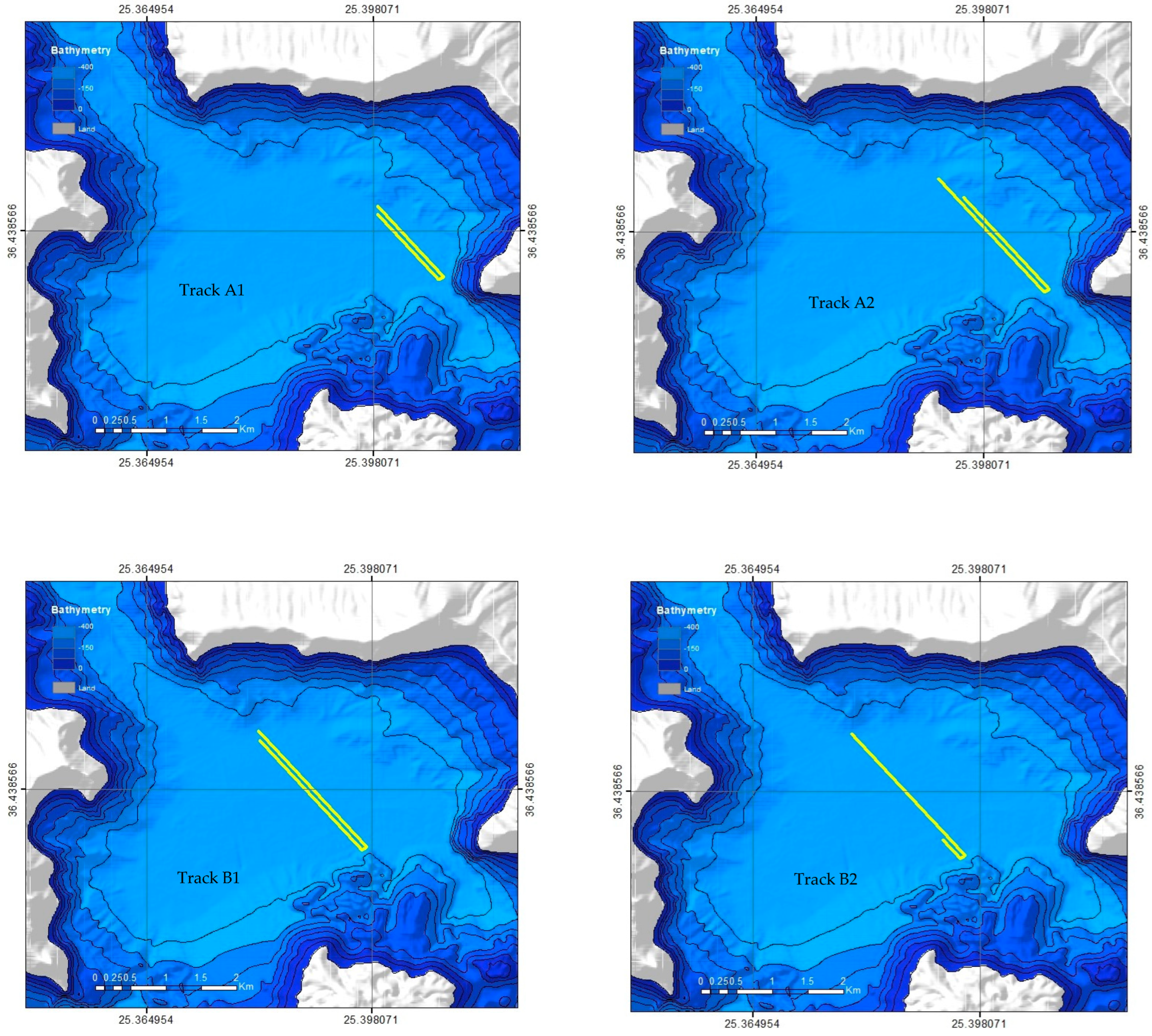
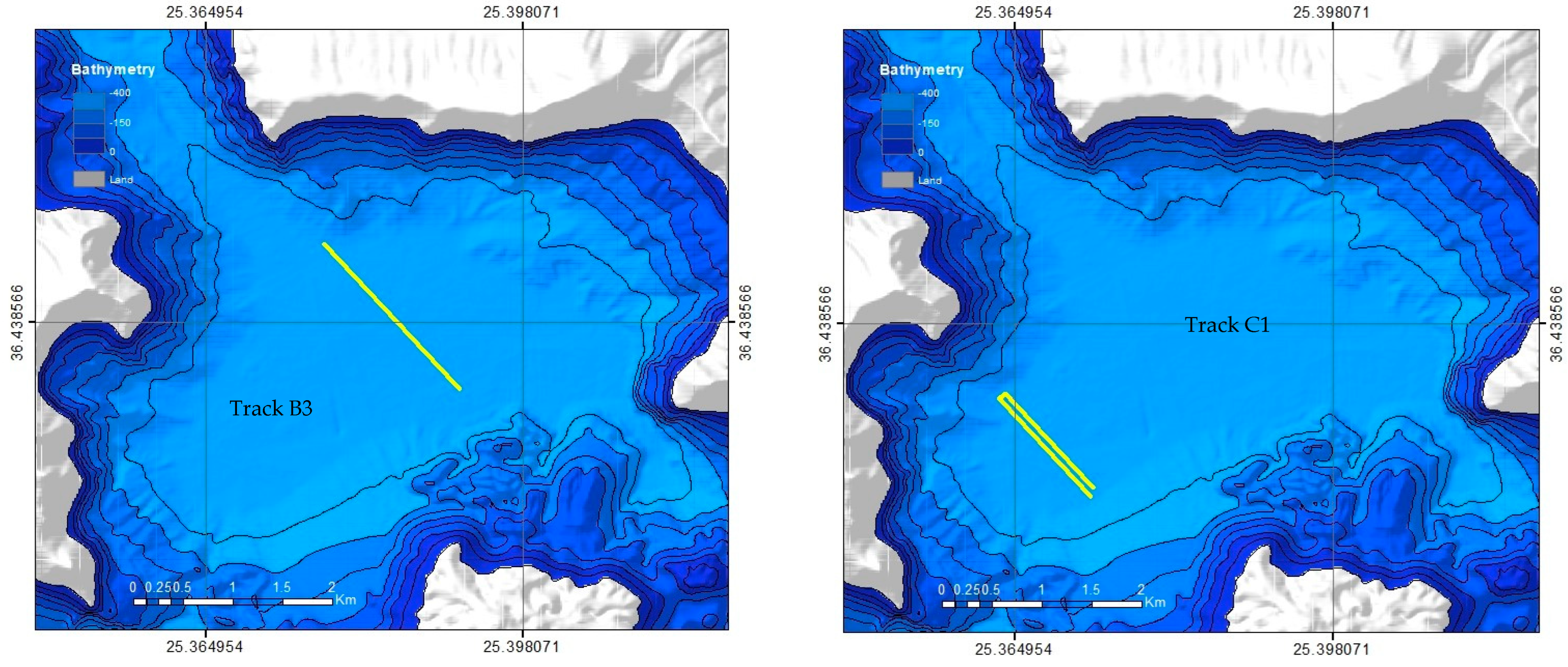
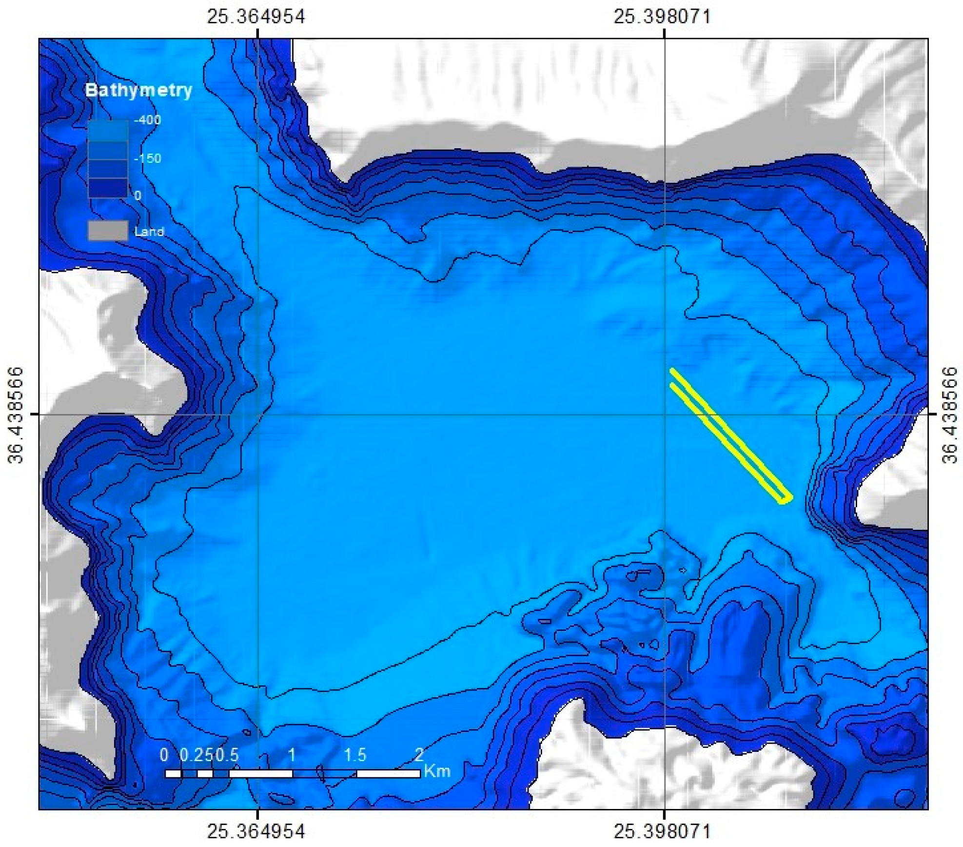
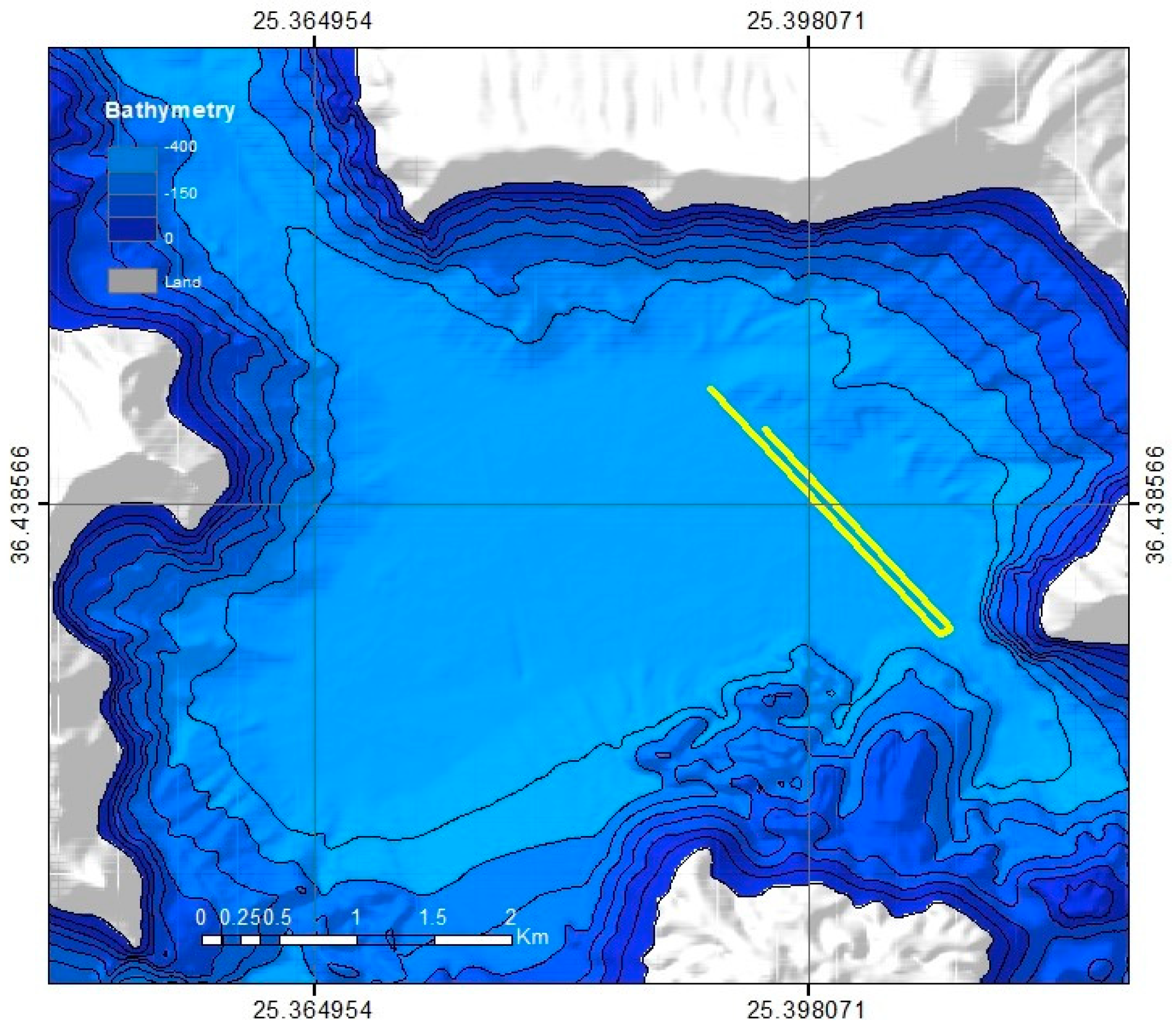
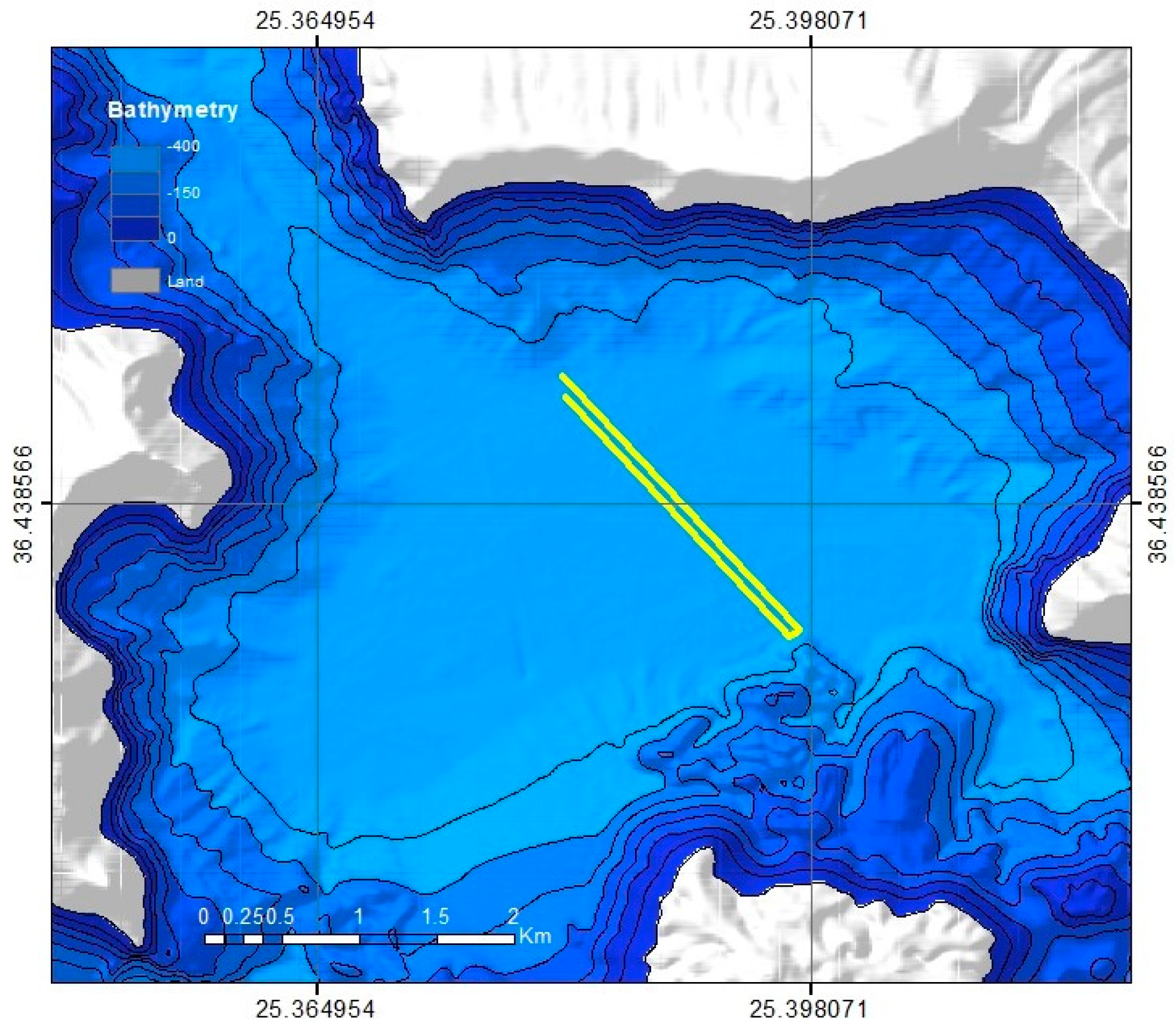
2.1. The Mission
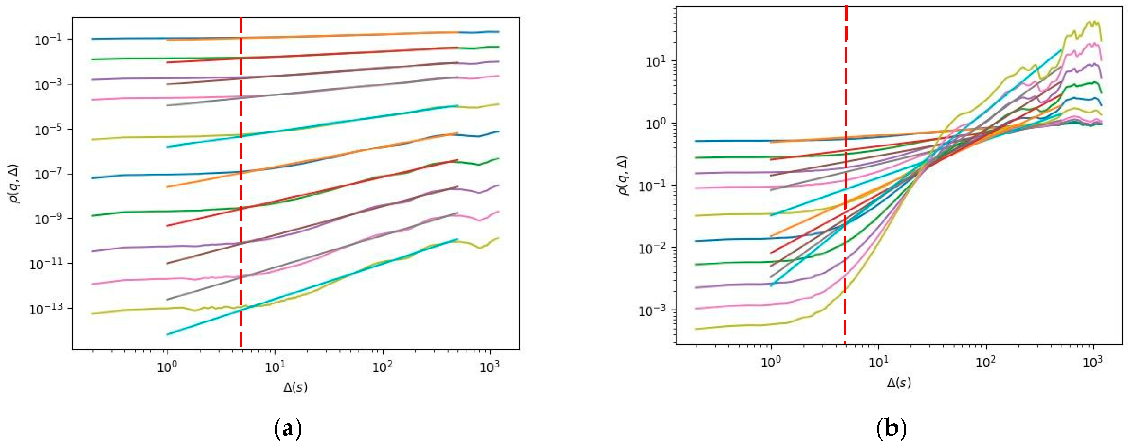
2.2. The Generalized Moments Method
- Construct a time series with different lag times.
- Estimate the statistical moments. See Equation (3).
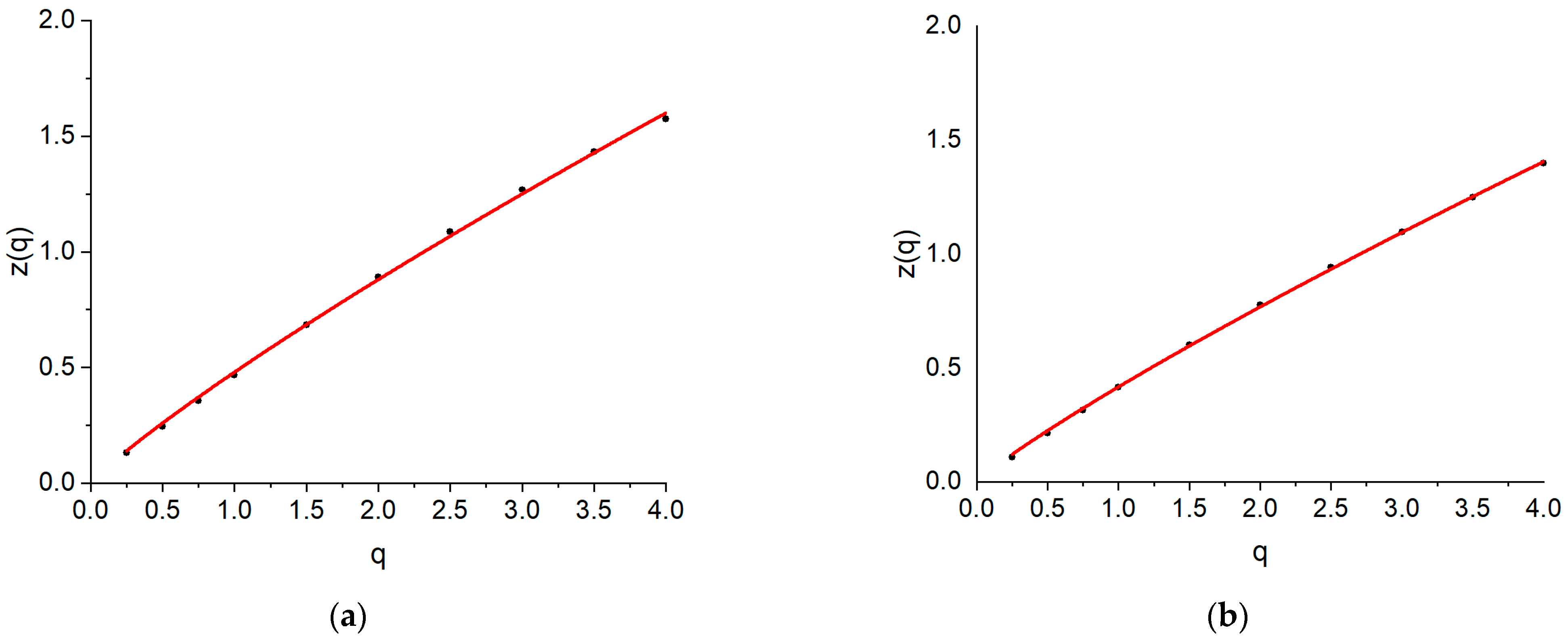
- Show the moments scale according to Equation (4).
3. Results
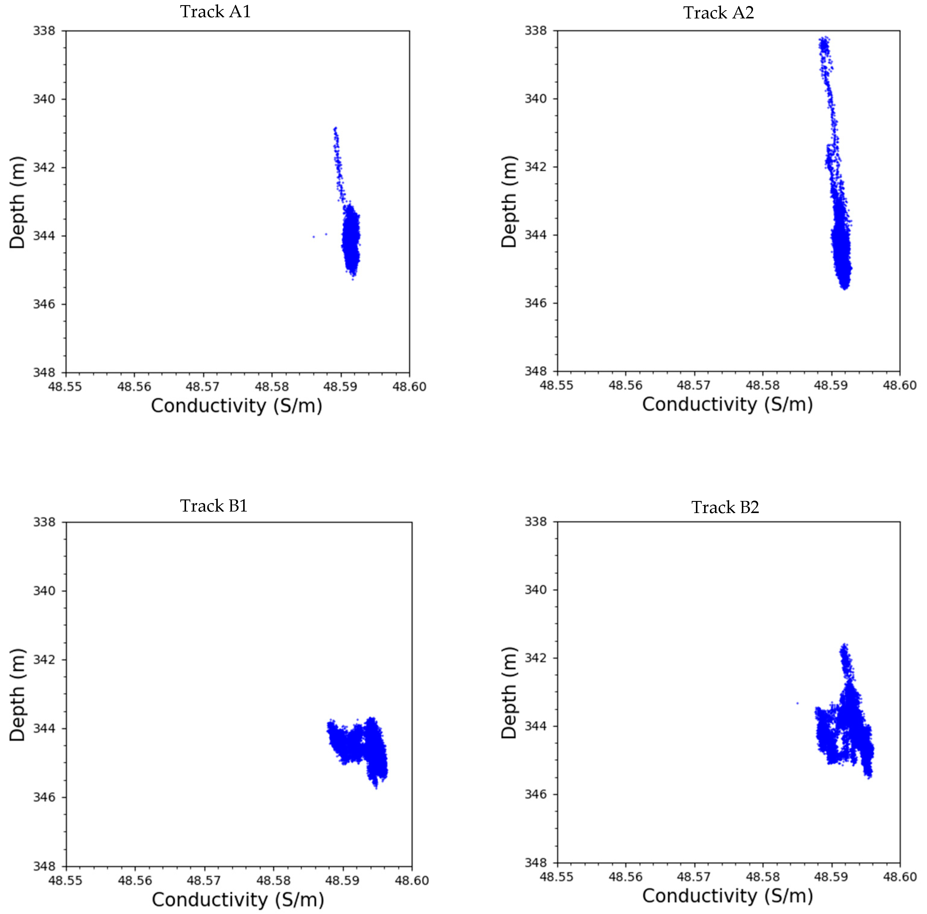
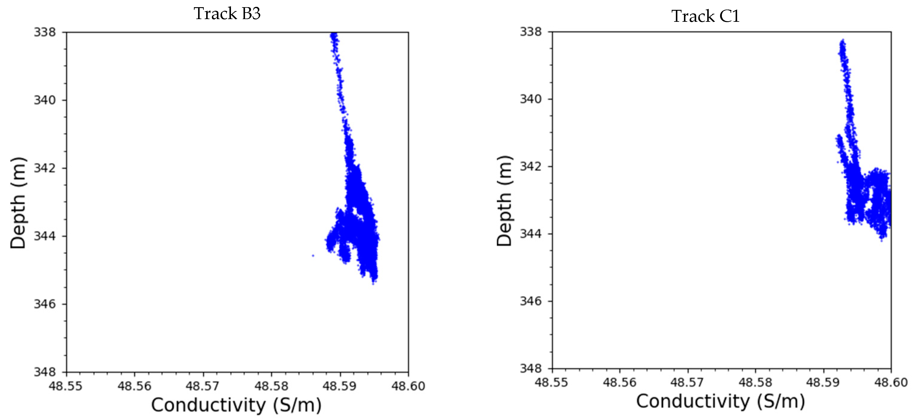
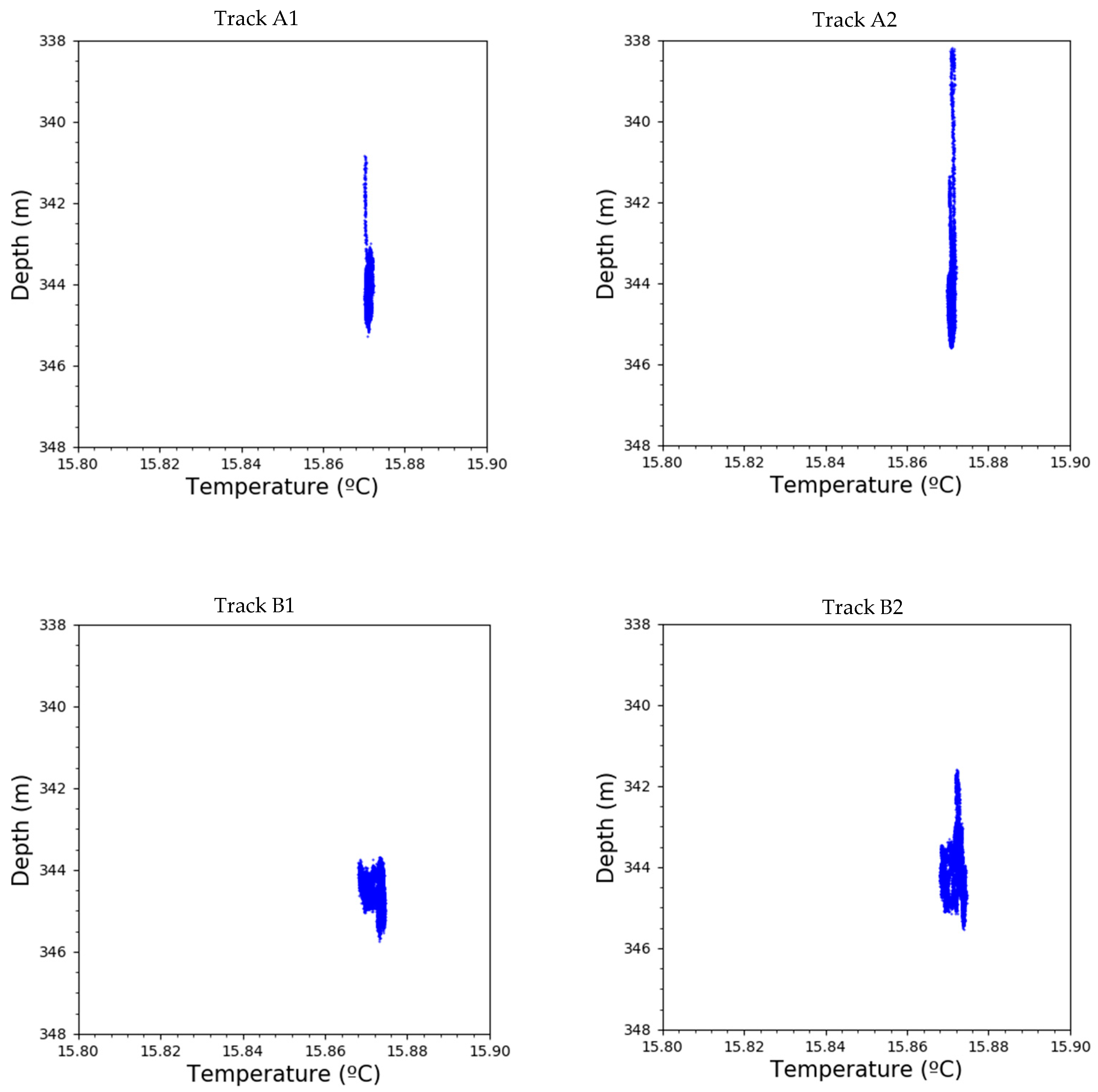
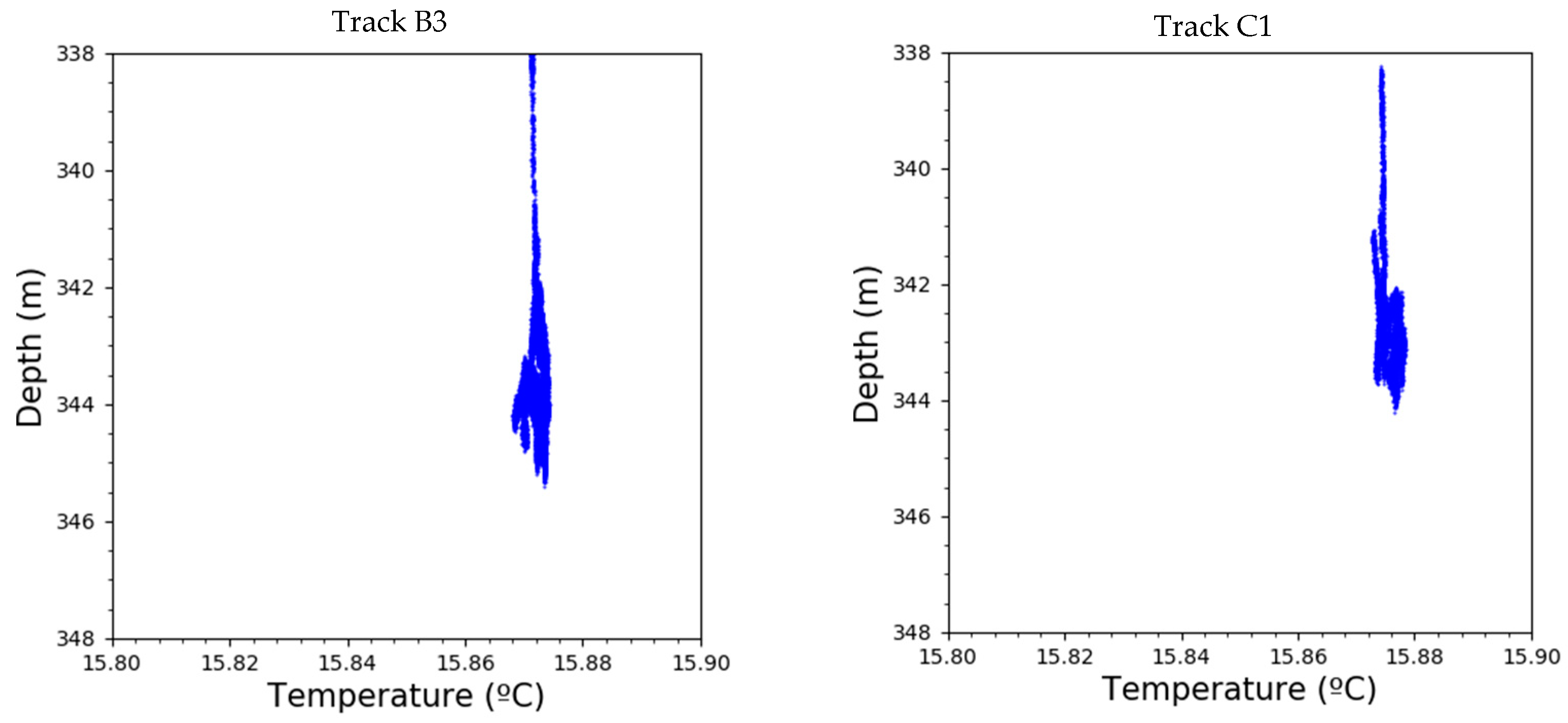
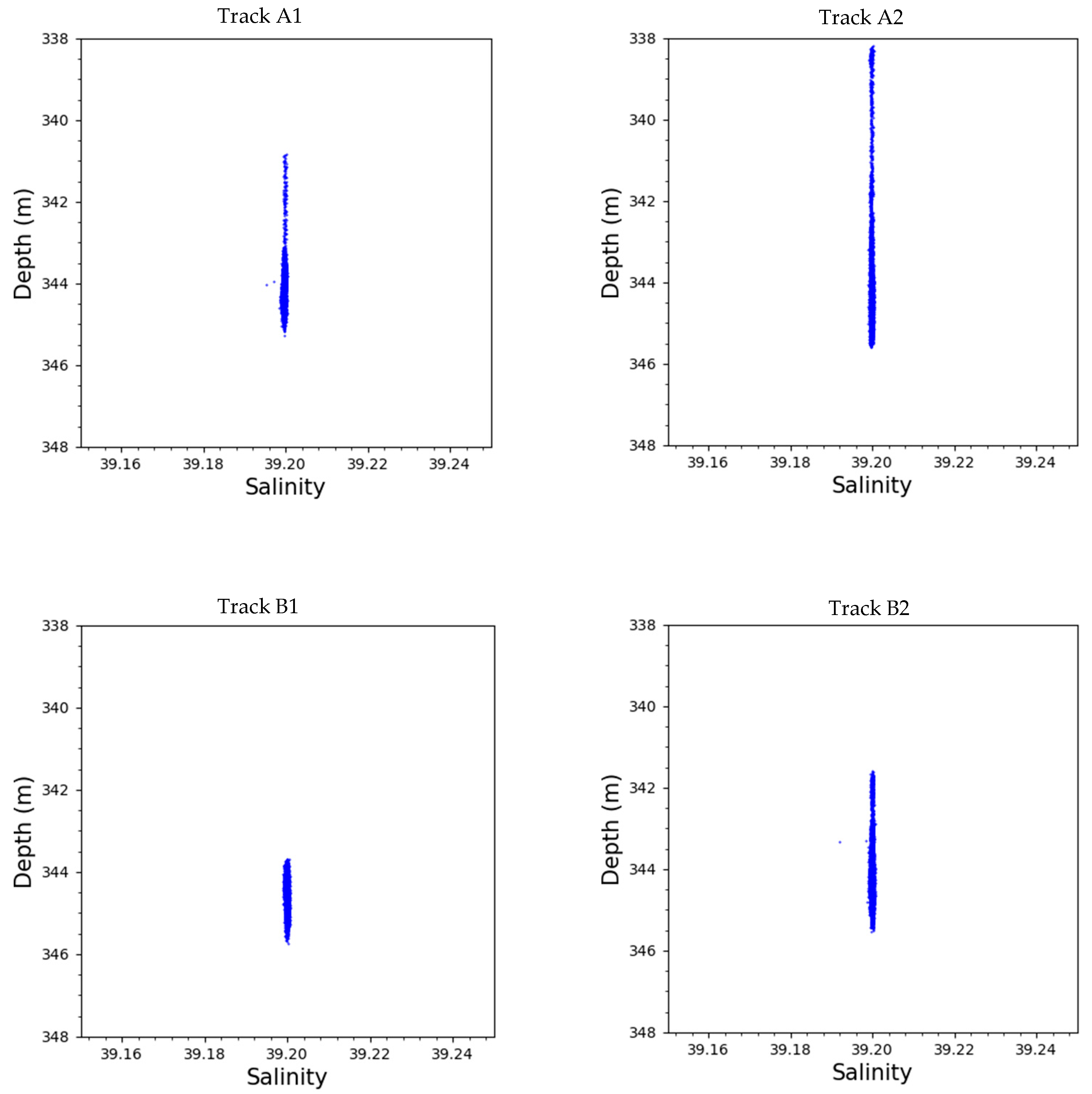
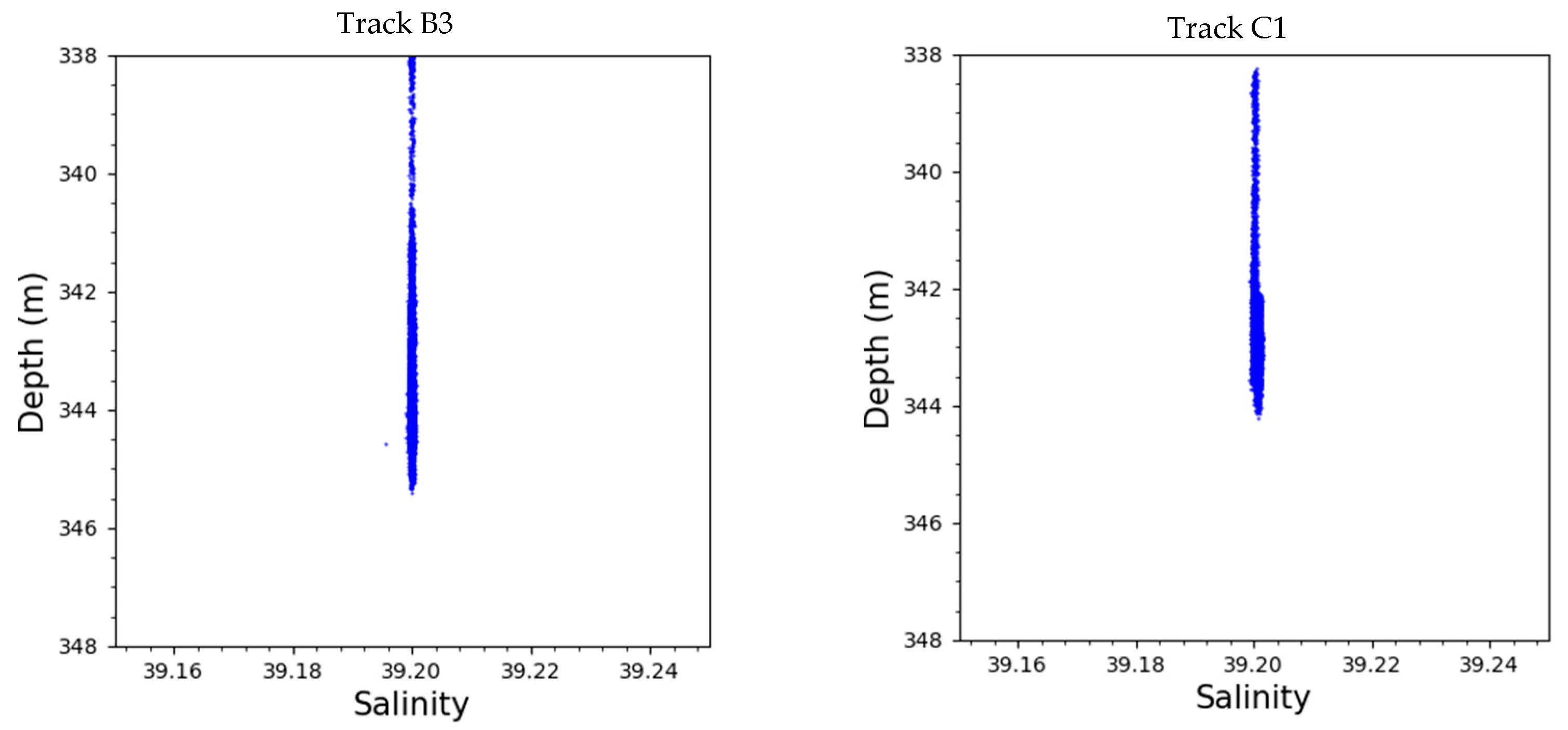
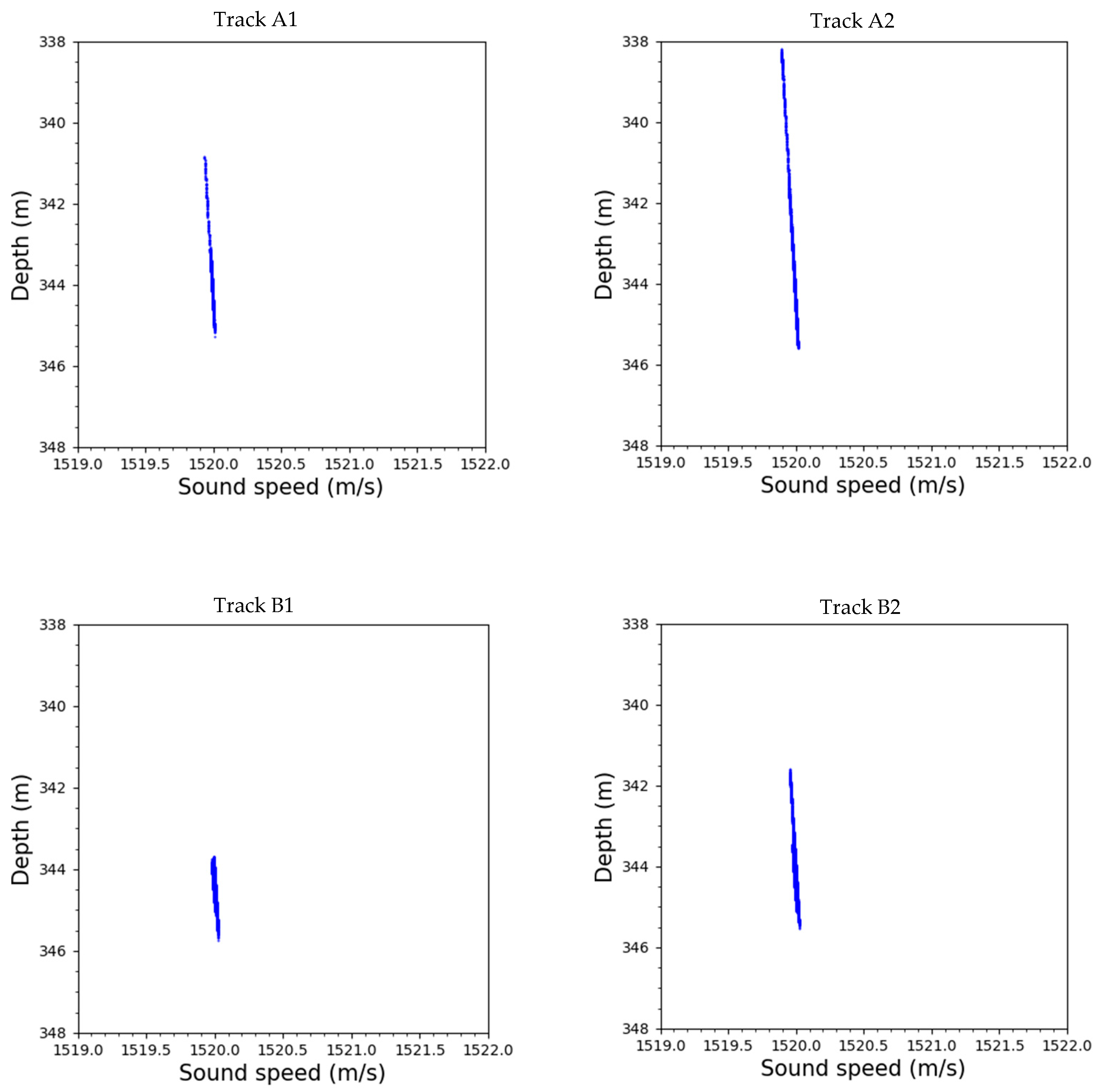
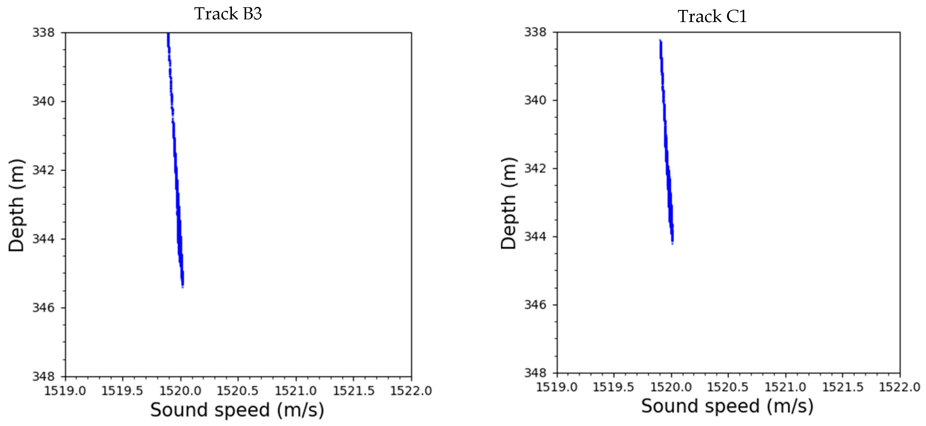
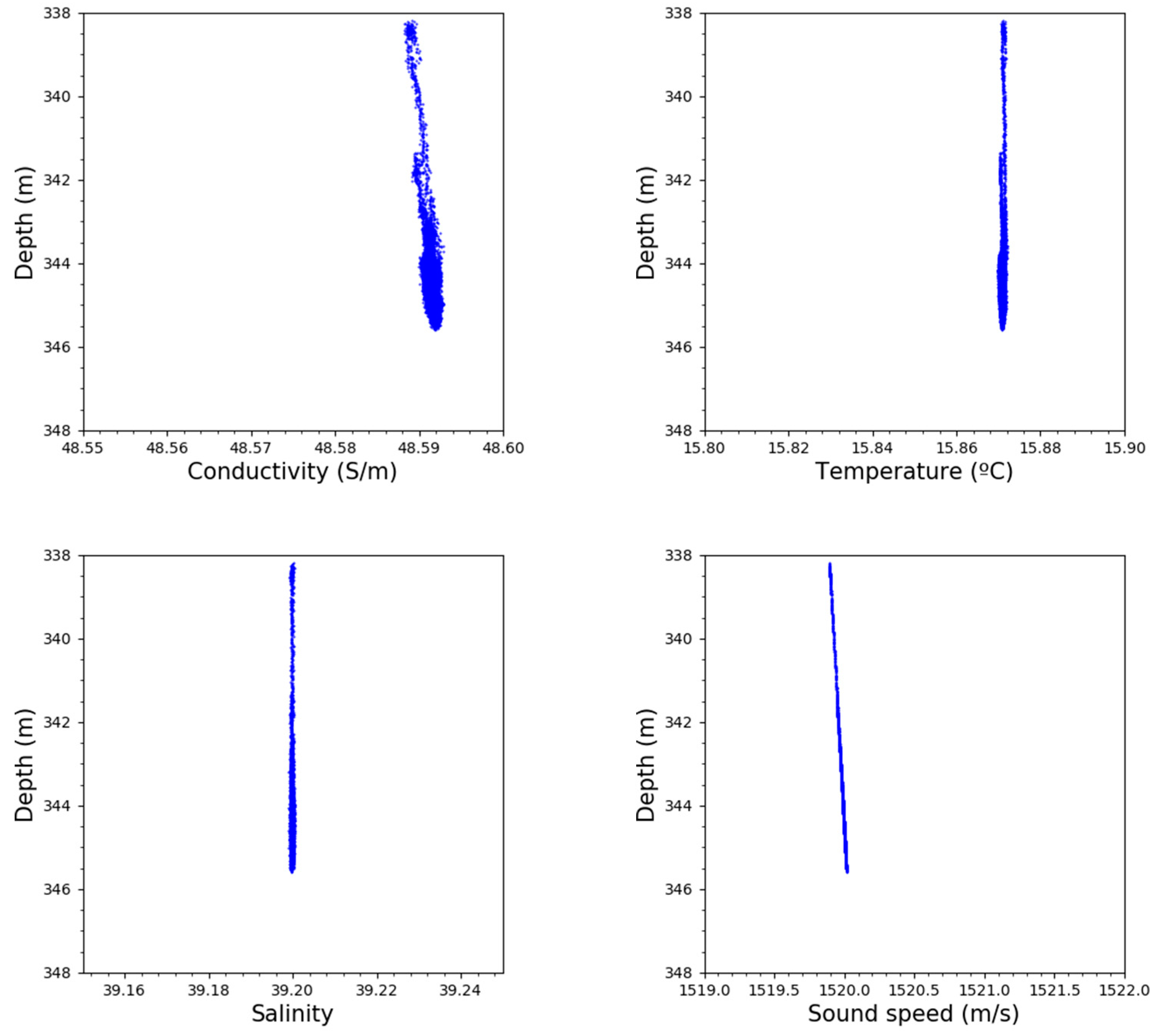
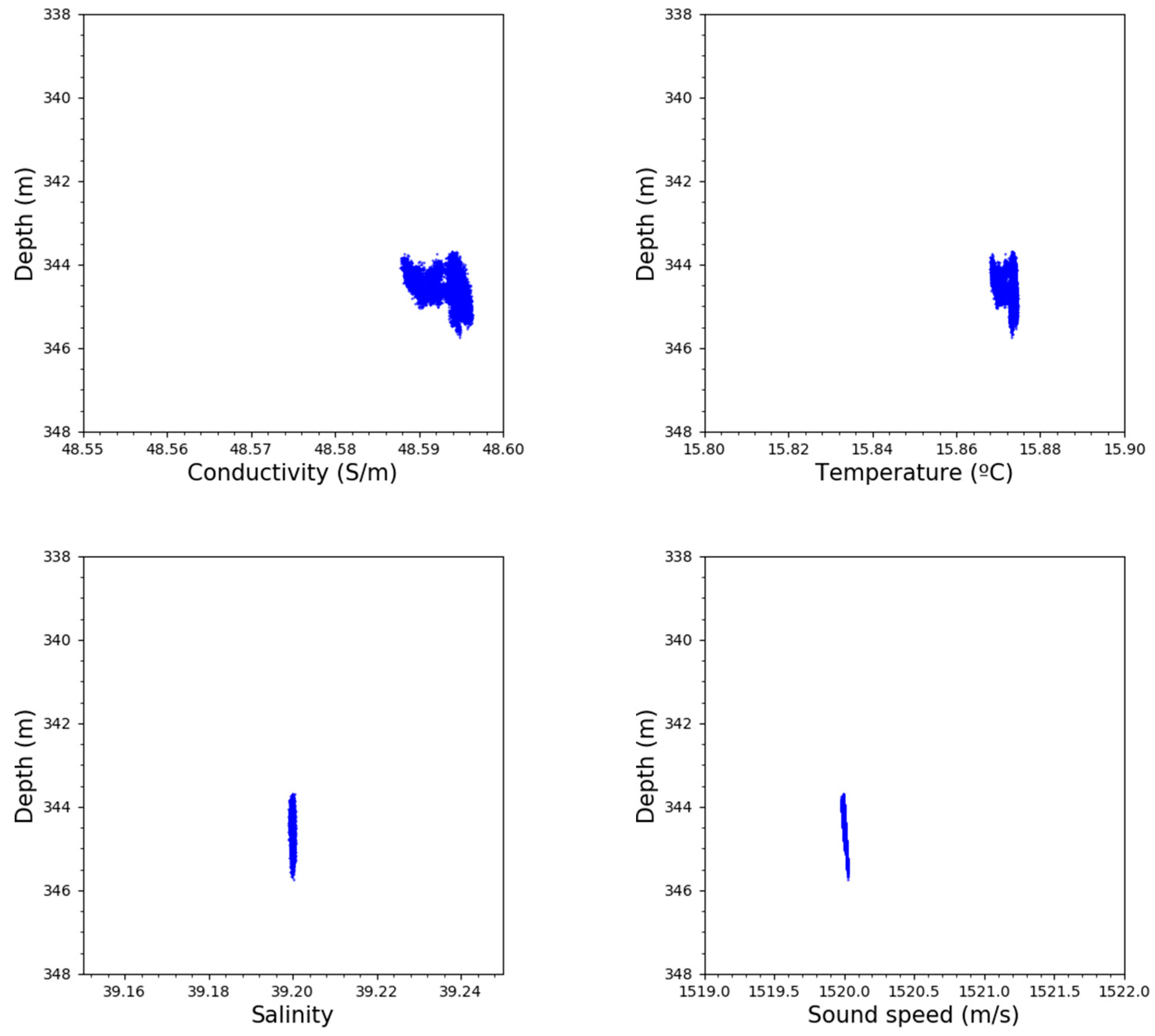
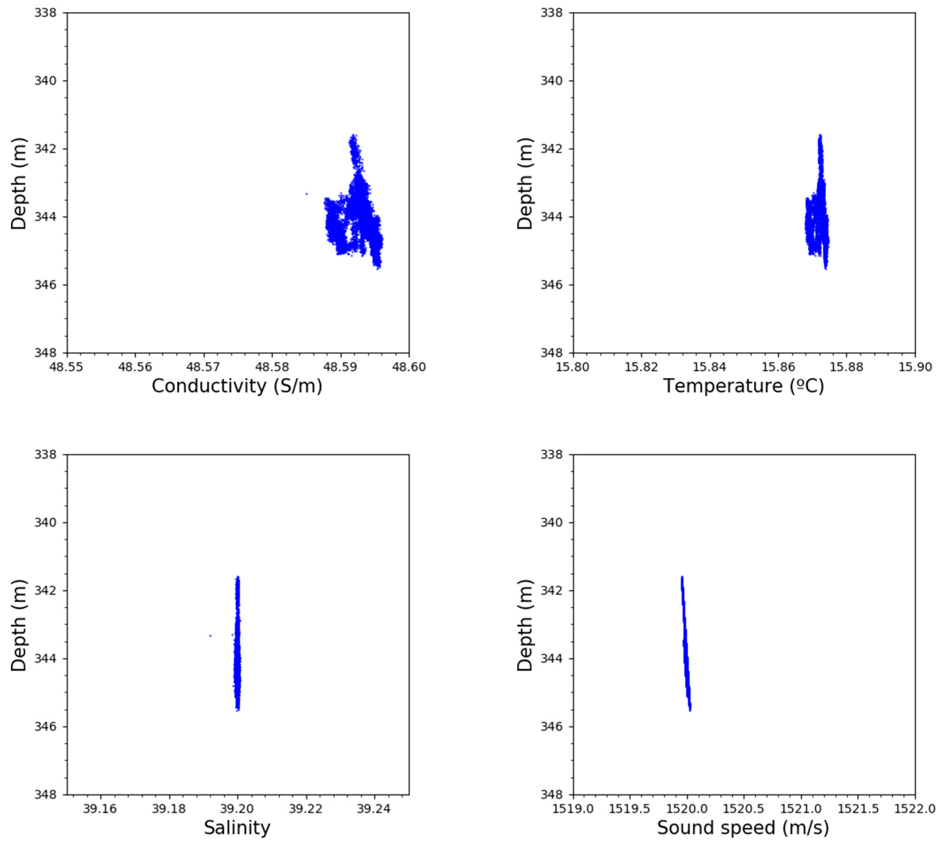
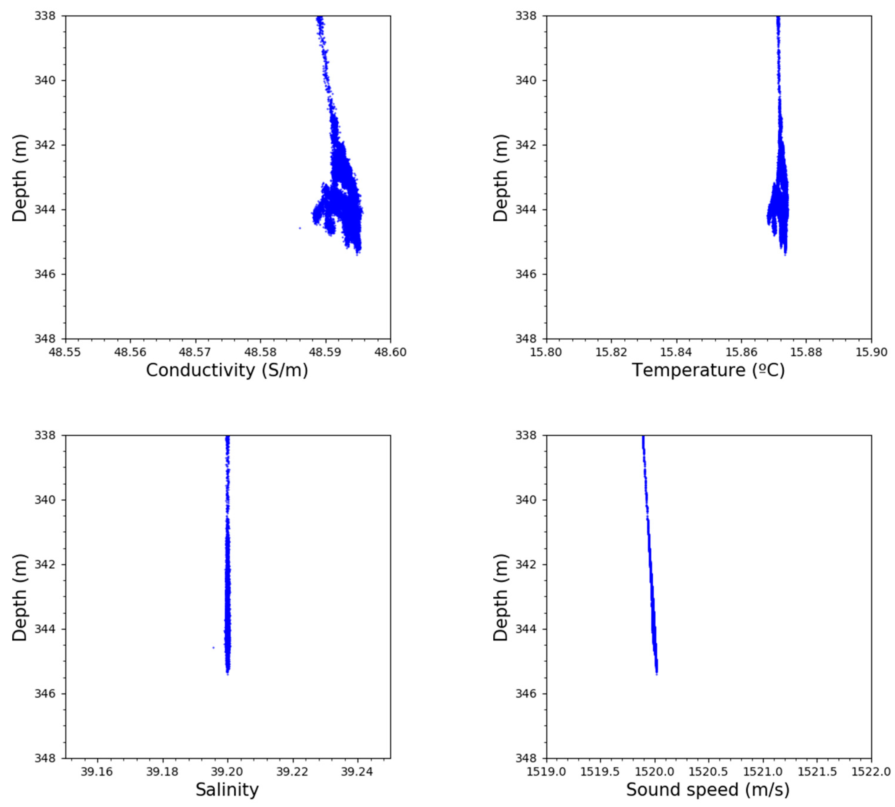
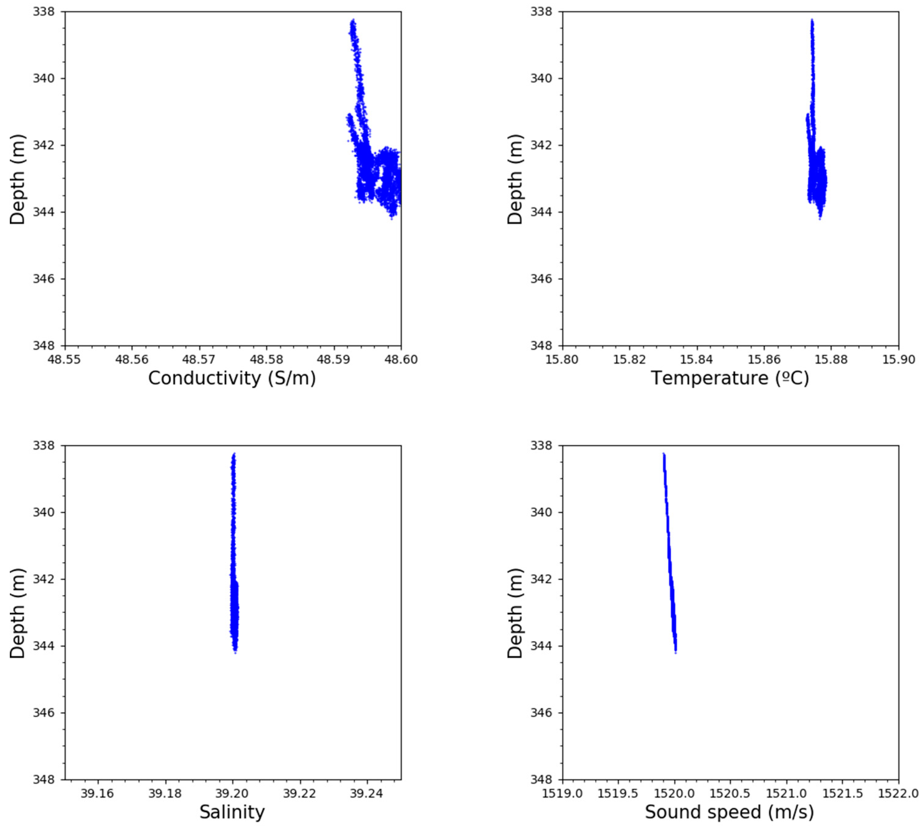
3.1. Depth Profiles
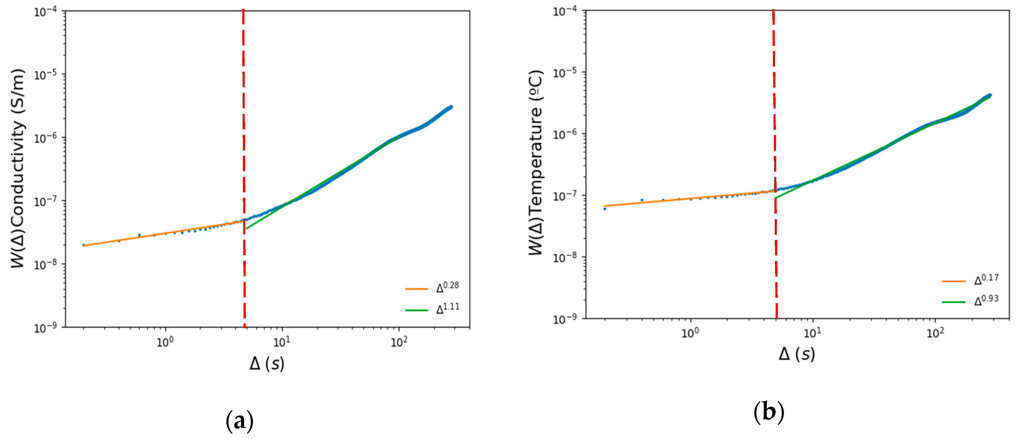
3.2. The Generalized Moments Method Results
4. Discussion
5. Conclusions
Author Contributions
Funding
Data Availability Statement
Acknowledgments
Conflicts of Interest
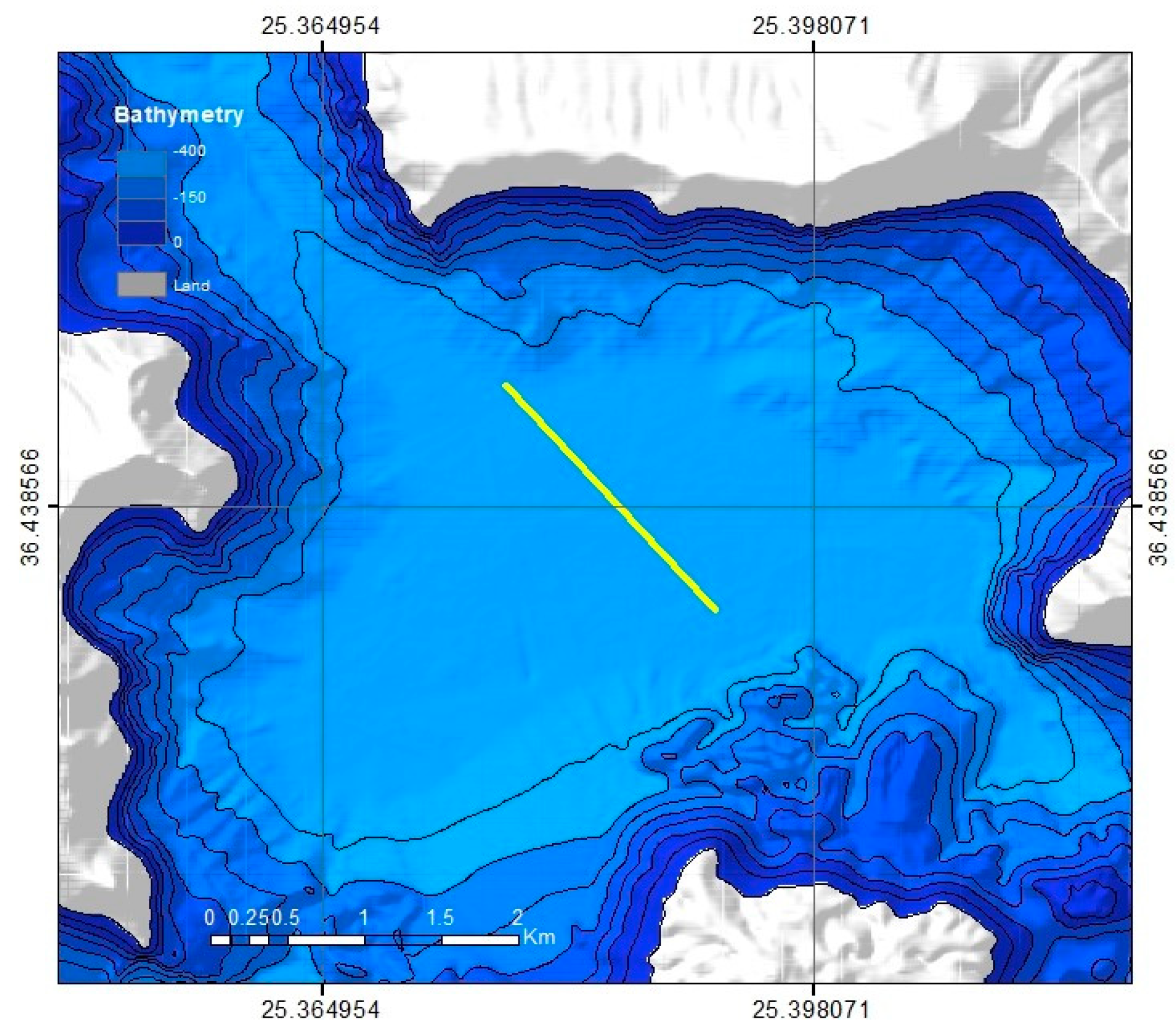
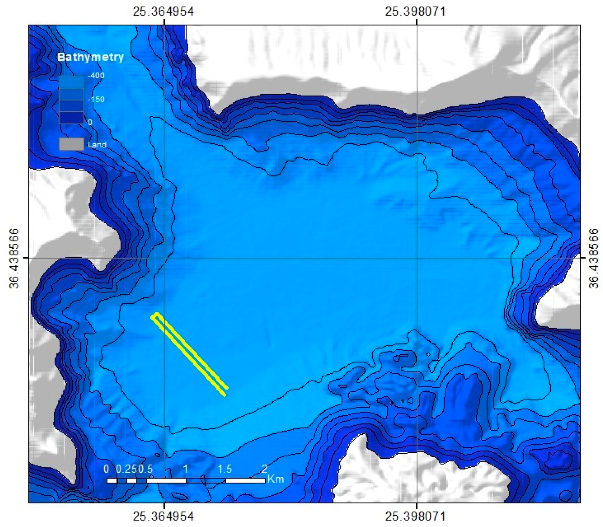
Appendix A. Autonomous Underwater Vehicle Tracks, Depth Profiles


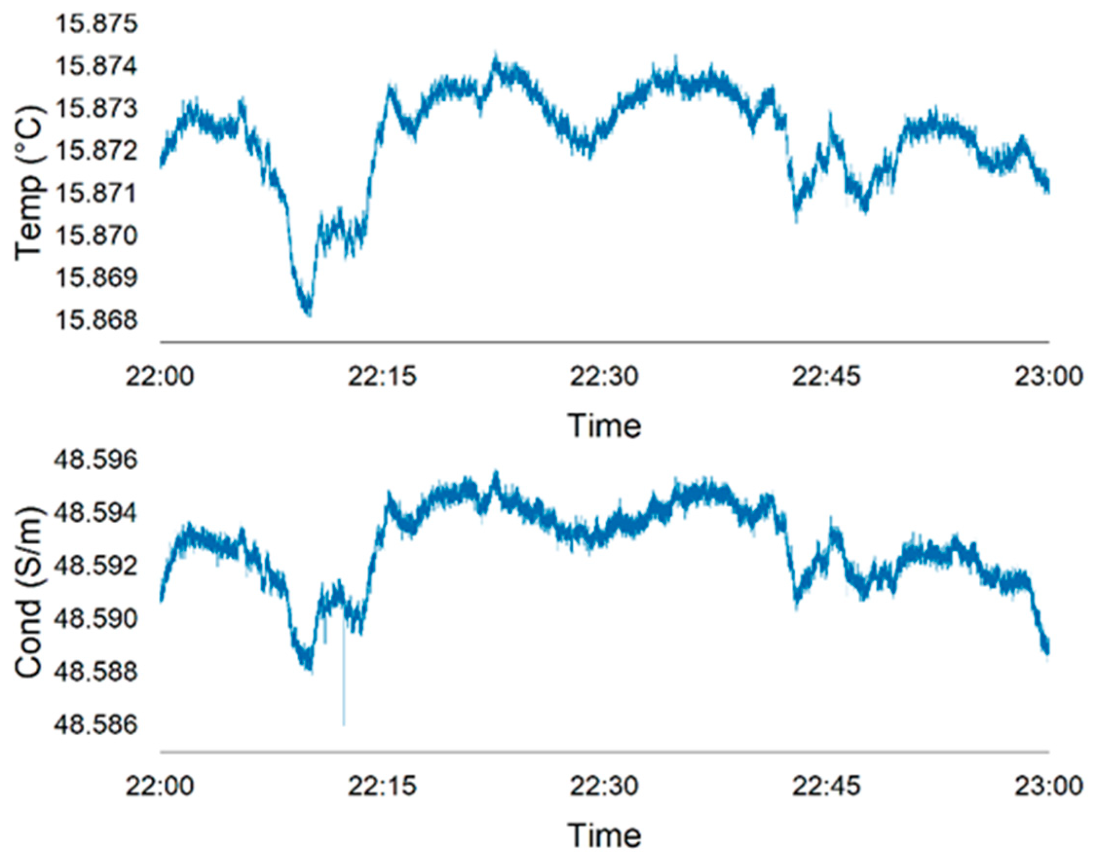
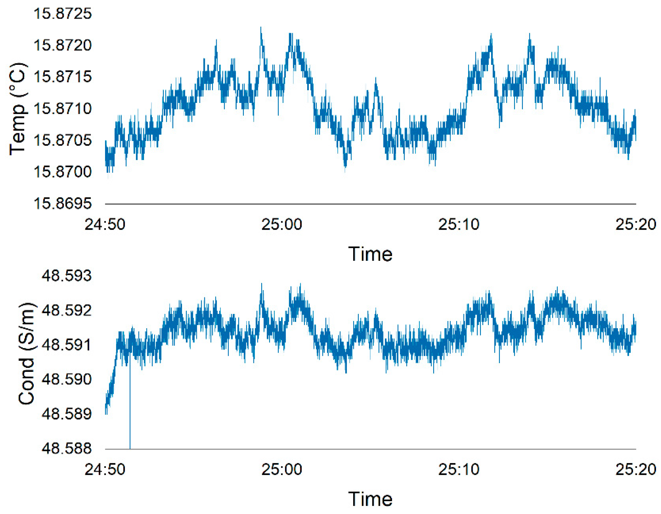
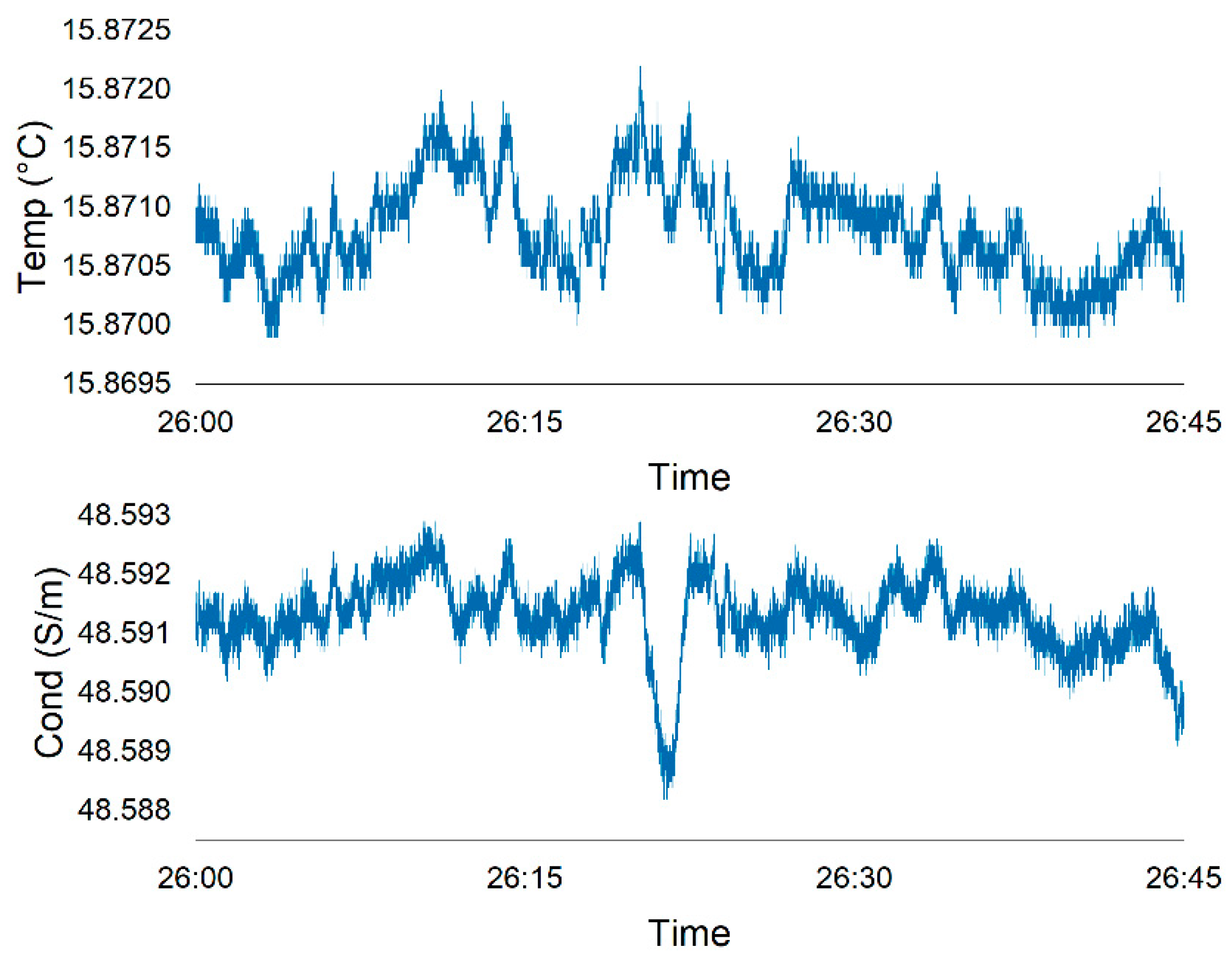
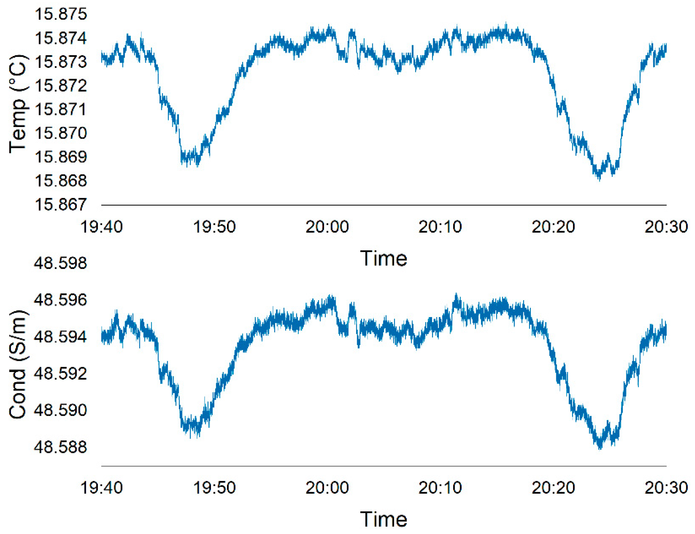
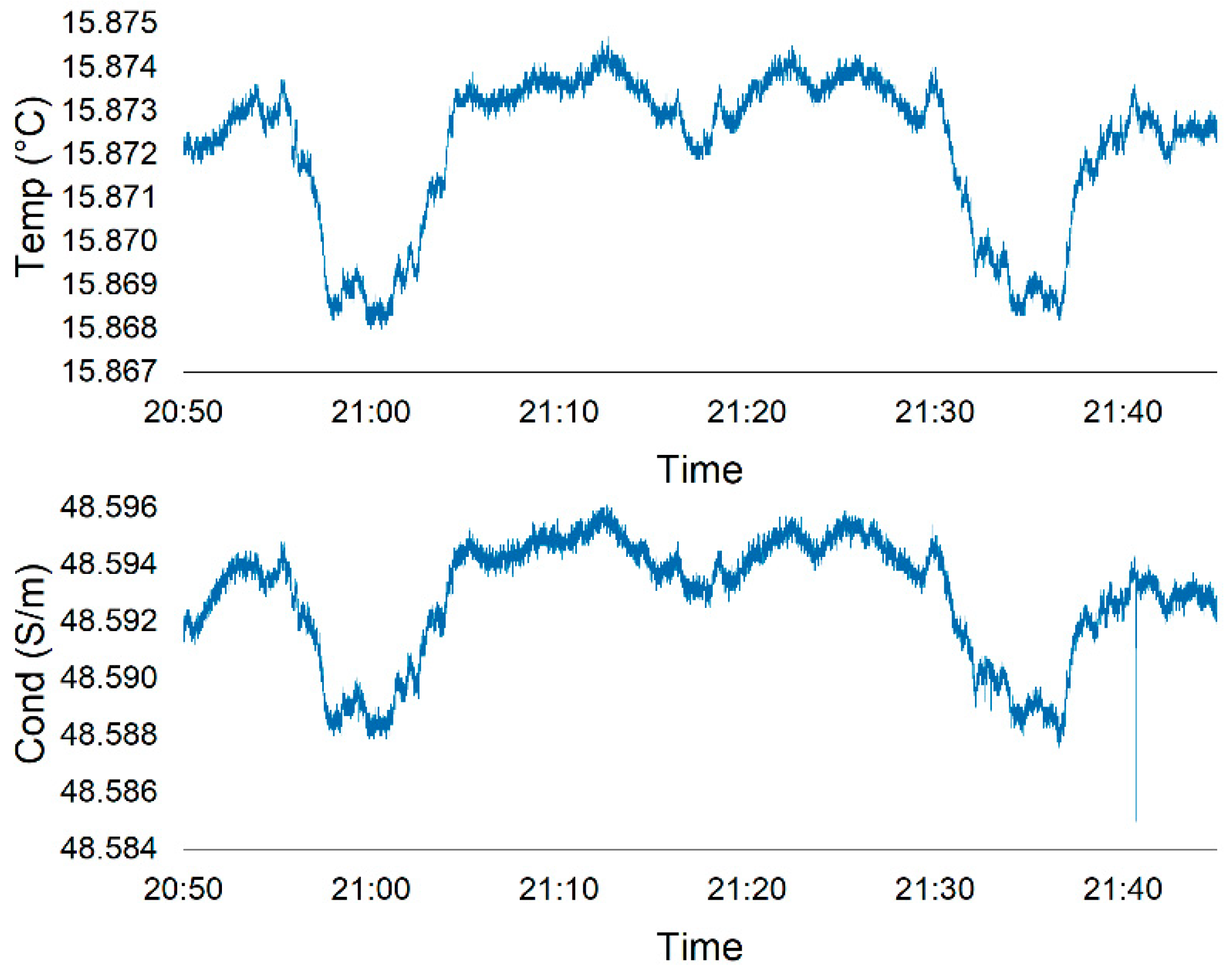
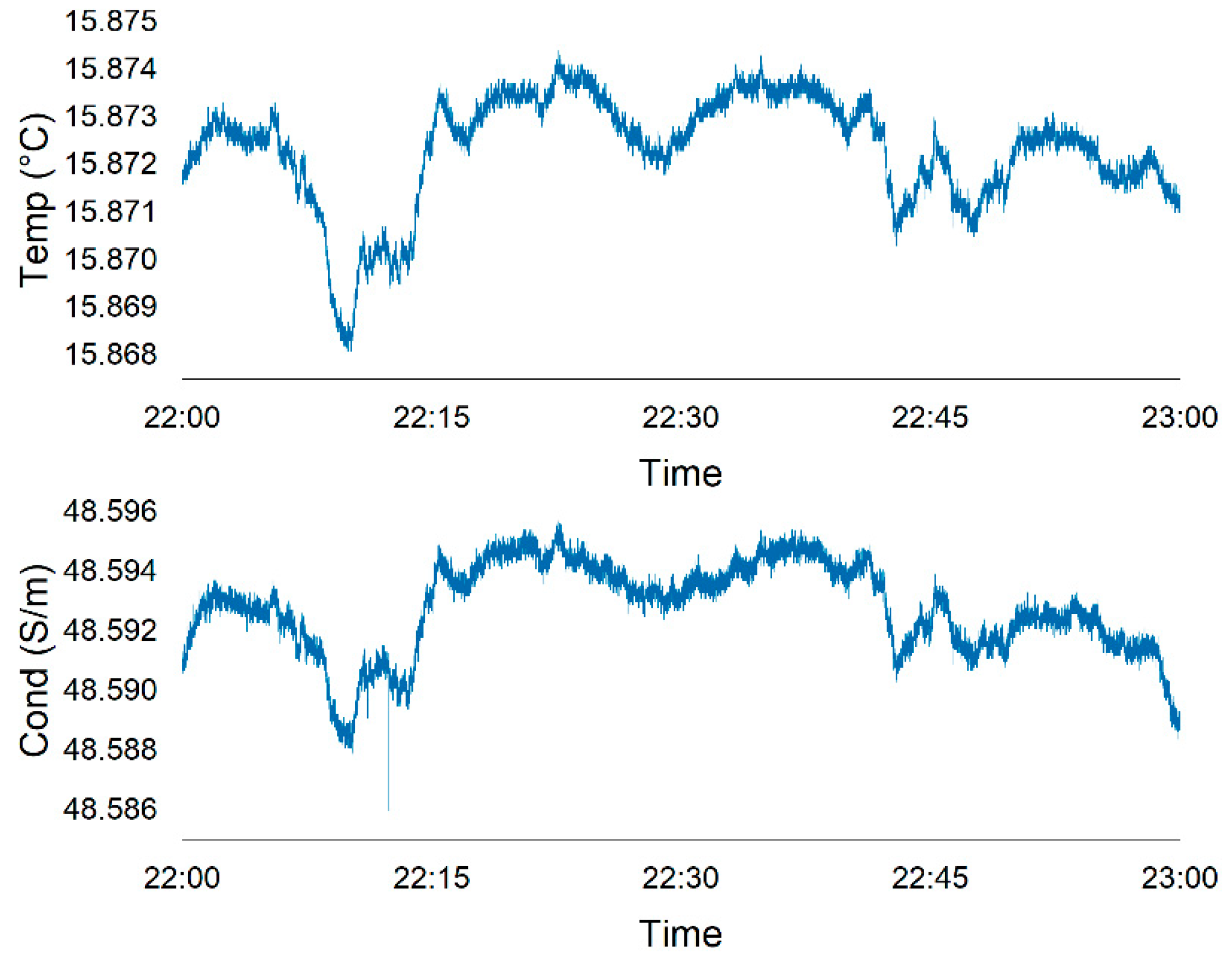
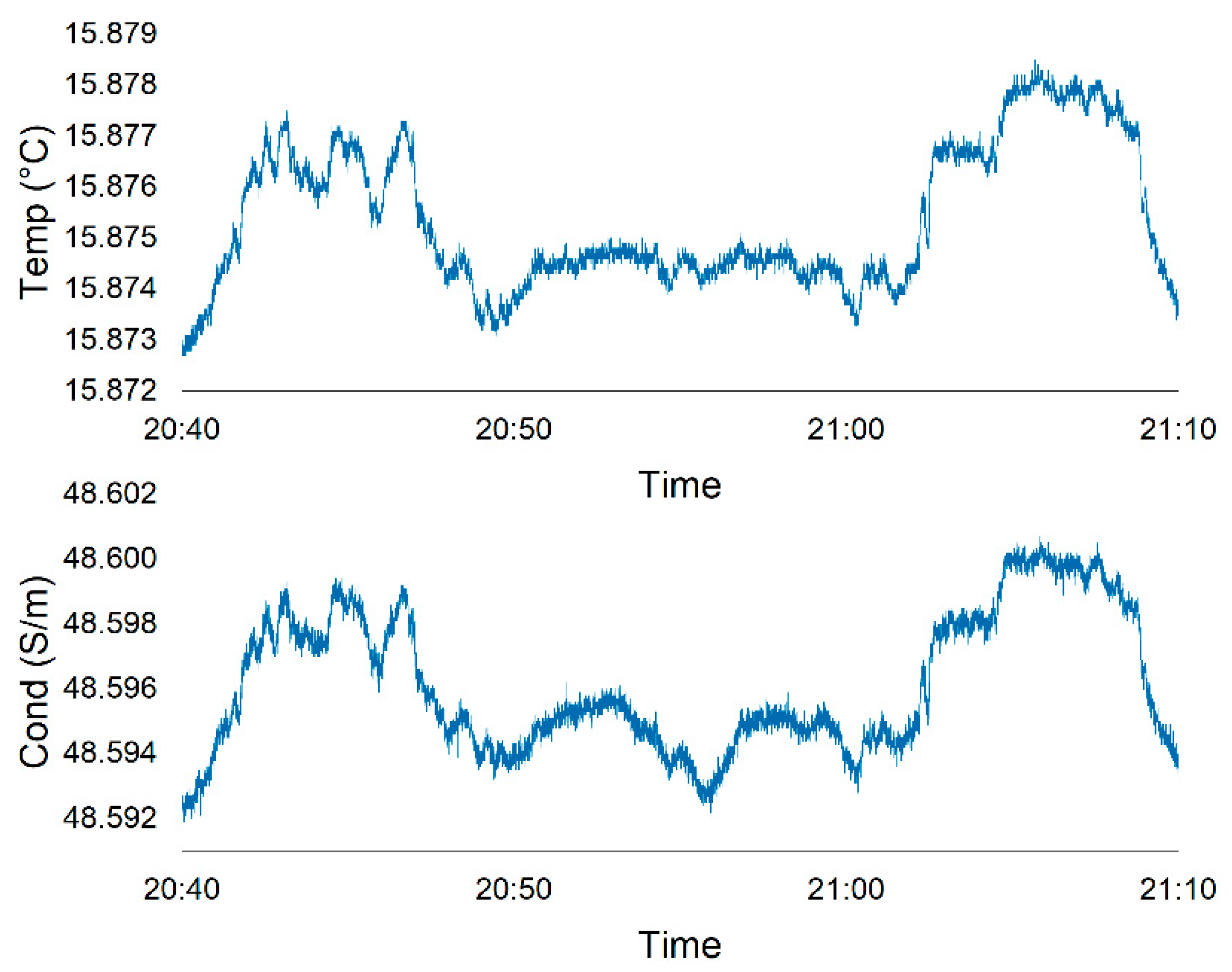
Appendix B. CTD Time Series


References
- Longchamp, C.; Bonadonna, C.; Bachmann, O.; Skopelitis, A. Characterization of tephra deposits with limited exposure: The example of the two largest explosive eruptions at Nisyros volcano (Greece). Bull. Volcanol. 2011, 73, 1337–1352. [Google Scholar] [CrossRef]
- Innocenti, F.; Manetti, P.; Peccerillo, A.; Poli, G. South Aegean volcanic arc: Geochemical variations and geotectonic implications. Bull Volcanol. 1981, 44, 377–391. [Google Scholar] [CrossRef]
- Papanikolaou, D. The Geology of Greece; Springer Nature: Basel, Switzerland, 2021. [Google Scholar]
- Reilinger, R.; McClusky, S.; Paradissis, D.; Ergintav, S.; Vernant, P. Geodetic constraints on the tectonic evolution of the Aegean region and strain accumulation along the Hellenic subduction zone. Tectonophysics 2010, 488, 22–30. [Google Scholar] [CrossRef]
- Papanikolaou, D. Geotectonic evolution of the Aegean. Bull. Geol. Soc. Greece 1993, XXVIII/1, 33–48. [Google Scholar]
- Pe-Piper, G.; Piper, D. The igneous rocks of Greece. The anatomy of an orogen. Gebrueder Borntreager 2002, 140, 357. [Google Scholar]
- Nomikou, P.; Papanikolaou, D.; Alexandri, M.; Sakellariou, D.; Rousakis, G. Submarine volcanoes along the Aegean volcanic arc. Tectonophysics 2013, 597–598, 123–146. [Google Scholar] [CrossRef]
- Nomikou, P.; Hübscher, C.; Carey, S. The Christiana–Santorini–Kolumbo volcanic field. Elements 2019, 15, 171–176. [Google Scholar] [CrossRef]
- Papanikolaou, D.; Nomikou, P. Tectonic structure and volcanic centres at the eastern edge of the Aegean volcanic arc around Nisyros Island. Bull. Geol. Soc. 2001, 34, 289–296. [Google Scholar]
- Nomikou, P.; Krassakis, P.; Kazana, S.; Papanikolaou, D.; Koukouzas, N. The volcanic relief within the kos-nisyros-tilos tectonic graben at the eastern edge of the aegean volcanic arc, greece and geohazard implications. Geosciences 2021, 11, 231. [Google Scholar] [CrossRef]
- Druitt, T.H.; Edwards, L.; Mellors, R.M.; Pyle, D.M.; Sparks, R.S.J.; Lanphere, M.; Davies, M.; Barreirio, A. Santorini Volcano. Geol. Soc. Lond. 1999, 19, 176. [Google Scholar]
- Nomikou, P.; Croff Bell, K.; Bejelou, K.; Parks, M.; Antoniou, V. ROV Exploration of Santorini Caldera, Greece. Manuscript 2010, 1866–1870. Available online: https://www.researchgate.net/profile/Paraskevi-Nomikou/publication/258618879_Submarine_Volcanic_Morphology_of_Santorini_Caldera_Greece/links/582dc7cb08ae004f74bcd5e9/Submarine-Volcanic-Morphology-of-Santorini-Caldera-Greece.pdf (accessed on 30 August 2023).
- Druitt, T.H.; Pyle, D.M.; Mather, T.A. Santorini volcano and its plumbing system. Elem. Int. Mag. Mineral. Geochem. Petrol. 2019, 15, 177–184. [Google Scholar] [CrossRef]
- Nomikou, P.; Druitt, T.H.; Hubscher, C.; Mather, T.A.; Paulatto, M.; Kalnins, L.M.; Kelfoun, K.; Papanikolaou, D.; Bejelou, K.; Lampridou, D.; et al. Post-eruptive flooding of Santorini caldera (Greece), and implica_tions for tsunami generation. Nat. Commun. 2016, 7, 13332. [Google Scholar] [CrossRef] [PubMed]
- Karstens, J.; Preine, J.; Carey, S.; Bell, K.L.C.; Nomikou, P.; Huebscher, C.; Lampridou, D.; Urlaub, M. Formation of undulating seafloor bedforms during the Minoan eruption and their implications for eruption dynamics and slope stability at Santorini. Earth Planet. Sci. Lett. Rev. 2023, 616, 118215. [Google Scholar] [CrossRef]
- Satow, C.; Gudmundsson, A.; Gertisser, R.; Ramsey, C.B.; Bazargan, M.; Pyle, D.M. Eruptive activity of the Santorini Volcano controlled by sea-level rise and fall. Nat. Geosci. 2021, 14, 586–592. [Google Scholar] [CrossRef]
- Heiken, G.; McCoy, F. Caldera development during the Minoan eruption, Thira, Cyclades, Greece. J. Geophys. Res. 1984, 89, 8441–8462. [Google Scholar] [CrossRef]
- Johnston, E.N.; Johnston, E.N.; Sparks, R.S.J.; Phillips, J.C.; Carey, S. Revised estimates for the volume of the Late Bronze Age Minoan eruption, Santorini, Greece. J. Geol. Soc. 2014, 171, 583–590. [Google Scholar] [CrossRef]
- Bond, A.; Sparks, R.S.J. The Minoan eruption of Santorini, Greece. J. Geol. Soc. Lond. 1976, 132, 1–16. [Google Scholar] [CrossRef]
- Druitt, T.H.; Francaviglia, V. Caldera formation on Santorini and the physiography of the islands in the late Bronze Age. Bull. Volcanol. 1992, 54, 484–493. [Google Scholar] [CrossRef]
- Pyle, D.; Elliott, J. Quantitative morphology, recent evolution, and future activity of the Kameni Islands volcano, Santorini, Greece. Geosphere 2006, 2, 253–268. [Google Scholar] [CrossRef]
- Sigurdsson, H.; Carey, S.; Alexandri, M.; Vougioukalakis, G.; Croff, K.; Roman, C.; Sakellariou, D.; Anagnostou, C.; Rousakis, G.; Ioakim, C.; et al. Marine investigations of Greece’s Santorini Volcanic Field. Eos 2006, 87, 337–339. [Google Scholar] [CrossRef]
- Camilli, R.; Nomikou, P.; Escartín, J.; Ridao, P.; Mallios, A.; Kilias, S.P.; Argyraki, A. The Kallisti Limnes, carbon dioxide-accumulating subsea pools. Nat. Sci. Rep. 2015, 5, 12152. [Google Scholar] [CrossRef] [PubMed]
- Nomikou, P.; Polymenakou, P.N.; Rizzo, A.L.; Petersen, S.; Hannington, M.; Kilias, S.P.; Papanikolaou, D.; Escartin, J.; Karantzalos, K.; Mertzimekis, T.J.; et al. SANTORY: SANTORini’s Seafloor Volcanic ObservatorY. Front. Mar. Sci. 2022, 9, 421. [Google Scholar] [CrossRef]
- Christopoulou, M.; Mertzimekis, T.J.; Nomikou, P.; Papanikolaou, D.; Carey, S.; Mandalakis, M. Influence of hydrothermal venting on water column properties in the crater of the Kolumbo submarine volcano, Santorini volcanic field (Greece). Geo-Mar. Lett. 2016, 36, 15–24. [Google Scholar] [CrossRef]
- Dura, A.; Mertzimekis, T.J.; Bakalis, E.; Nomikou, P.; Gondikas, A.; Hannington, M.D.; Petersen, S. CTD data profiling to assess the natural hazard of active submarine vent fields: The case of Santorini Island. Ext. Abs. GSG2019-213. Bull. Geol. Soc. Greece Sp. Pub. 2020, 7, 620–621. [Google Scholar]
- Hannington, M.D. RV POSEIDON Fahrtbericht/Cruise Report POS510—ANYDROS: Rifting and Hydrothermal Activity in the Cyclades Back-Arc Basin, Catania (Italy)—Heraklion (Greece) 06.03.-29.03.2017; GEOMAR Report; N. Ser. 043; GEOMAR Helmholtz-Zentrum für Ozeanforschung: Kiel, Germany, 2018. [Google Scholar] [CrossRef]
- Zivot, E.; Wang, J. Generalized Method of Moments. In Modeling Financial Time Series with S-PLUS®; Zivot, E., Wang, J., Eds.; Springer: New York, NY, USA, 2006; pp. 785–845. [Google Scholar]
- Hansen, L. Large Sample Properties of Generalized Method of Moments Estimators. Econometrica 1982, 50, 1029–1054. [Google Scholar] [CrossRef]
- Nurhidayat, Y. An Application of Generalized Moments Method to Examine the Management Behavior during Peak Season A Study in Islamic Micro Finance Industry. MATEC Web Conf. 2018, 218, 04025. [Google Scholar] [CrossRef][Green Version]
- Lovejoy, S.; Schertzer, D. Multifractals and rain. In New Uncertainty Concepts in Hydrology and Water Resources; Cambridge University Press: Cambridge, UK, 1995; pp. 61–103. [Google Scholar]
- Schertzer, D.; Lovejoy, S. Multifractals, generalized scale invariance and complexity in geophysics. Int. J. of Bifurc. Chaos 2011, 21, 3417–3456. [Google Scholar] [CrossRef]
- Bakalis, E.; Mertzimekis, T.J.; Nomikou, P.; Zerbetto, F. Breathing modes of Kolumbo submarine volcano (Santorini, Greece). Sci. Rep. 2017, 7, 46515. [Google Scholar] [CrossRef]
- Bakalis, E.; Mertzimekis, T.J.; Nomikou, P.; Zerbetto, F. Temperature and conductivity as indicators of the morphology and activity of a submarine volcano: Avyssos (nisyros) in the south aegean sea, Greece. Geosciences 2018, 8, 193. [Google Scholar] [CrossRef]
- Dura, A.; Mertzimekis, T.J.; Nomikou, P.; Gondikas, A.; Gómez Míguez, M.M.; Bakalis, E.; Zerbetto, F. The hydrothermal vent field at the eastern edge of the hellenic volcanic arc: The avyssos caldera (nisyros). Geosciences 2021, 11, 290. [Google Scholar] [CrossRef]
- Olivé Abelló, A.; Vinha, B.; Machín, F.; Zerbetto, F.; Bakalis, E.; Fraile-Nuez, E. Temperature and conductivity anomalies as a proxy for volcanic activity at the Tagoro submarine volcano in the Canary Islands. Int. Symp. Mar. Sci. 2020, VII, 1–23. [Google Scholar]
- Olivé Abelló, A.; Vinha, B.; Machín, F.; Zerbetto, F.; Bakalis, E.; Fraile-Nuez, E. Analysis of volcanic thermohaline fluctuations of tagoro submarine volcano (El Hierro Island, canary islands, Spain). Geosciences 2021, 11, 374. [Google Scholar] [CrossRef]
- Nomikou, P.; Carey, S.; Papanikolaou, D.; Croff Bell, K.; Sakellariou, D.; Alexandri, M.; Bejelou, K. Submarine volcanoes of the Kolumbo volcanic zone NE of Santorini Caldera, Greece. Glob. Planet. Chang. 2012, 90–91, 135–151. [Google Scholar] [CrossRef]
- Nomikou, P.; Parks, M.M.; Papanikolaou, D.; Pyle, D.M.; Mather, T.A.; Carey, S.; Watts, A.B.; Paulatto, M.; Kalnins, M.L.; Livanos, I.; et al. The emergence and growth of a submarine volcano: The Kameni islands, Santorini (Greece). Geo. Res. J. 2014, 1–2, 8–18. [Google Scholar] [CrossRef]
- Kantelhardt, J.; Zschiegner, S.; Koscielny-Bunde, E.; Havlin, S.; Bunde, A.; Stanley, H. Multifractal detrended fluctuation analysis of nonstationary time series. Physica A 2002, 316, 87–114. [Google Scholar] [CrossRef]
- Barunik, J.; Kristoufek, L. On Hurst exponent estimation under heavy-tailed distributions. Phys. A 2010, 389, 3844–3855. [Google Scholar] [CrossRef]
- Bakalis, E.; Höfinger, S.; Venturini, A.; Zerbetto, F. Crossover of two power laws in the anomalous diffusion of a two lipid membrane. J. Chem. Phys. 2015, 142, 215102. [Google Scholar] [CrossRef]
- Seuront, L.; Stanley, H.E. Anomalous diffusion and multifractality enhance mating encounters in the ocean. Proc. Natl. Acad. Sci. USA 2014, 111, 2206–2211. [Google Scholar] [CrossRef]
- Flandrin, P. On the Spectrum of Fractional Brownian Motions. IEEE Trans. Inf. Theory 1989, 35, 197–199. [Google Scholar] [CrossRef]
- Schertzer, D.; Lovejoy, S. Physical modeling and analysis of rain and clouds by anisotropic scaling multiplicative processes. J. Geophys. Res. 1987, 92, 9693–9714. [Google Scholar] [CrossRef]
- Schertzer, D.; Lovejoy, S. Universal Multifractals Do Exist! Comments on “A Statistical Analysis of 483 Mesoscale Rainfall as a Random Cascade”. J. Appl. Meteorol. 1997, 36, 1296–1303. [Google Scholar] [CrossRef]
- Ulvrova, M.; Paris, R.; Nomikou, P.; Kelfoun, K.; Leibrandt, S.; Tappin, D.R.; McCoy, F.W. Source of the tsunami generated by the 1650 AD eruption of Kolumbo submarine volcano (Aegean Sea, Greece). J. Volcanol. Geotherm. Res. 2016, 321, 125–139. [Google Scholar] [CrossRef]
- Nomikou, P.; Papanikolaou, D. The morphotectonic structure of Kos-Nisyros-Tilos volcanic area based on onshore and offshore data. In Proceedings of XIX Congr. Carpathian-Balk. Geol. Assoc. 2010, 99, 557–564. [Google Scholar]
- Nomikou, P.; Papanikolaou, D. A comparative morphological study of the Kos-Nisyros-Tilos volcanosedimentary basins. Bull. Geol. Soc. Greece 2010, 43, 464–474. [Google Scholar] [CrossRef][Green Version]
- Kilias, S.P.; Nomikou, P.; Papanikolaou, D.; Polymenakou, P.N.; Godelitsas, A.; Argyraki, A.; Carey, S.; Gamaletsos, P.; Mertzimekis, T.J.; Stathopoulou, E.; et al. New insights into hydrothermal vent processes in the unique shallow-submarine arc-volcano, Kolumbo (Santorini), Greece. Sci. Rep. 2013, 3, 2421. [Google Scholar] [CrossRef]


| Tracks | Time | Total Time (in Mins) |
|---|---|---|
| Track A1 | 24:50–25:20 | 30 |
| Track A2 | 26:00–26:45 | 45 |
| Track B1 | 19:40–20:30 | 50 |
| Track B2 | 20:50–21:45 | 55 |
| Track B3 | 22:00–23:00 | 60 |
| Track C1 | 20:40–21:10 | 30 |
| Tracks | 1st Regime | 2nd Regime | ||
|---|---|---|---|---|
| Conductivity | Temperature | Conductivity | Temperature | |
| Track A1 | 0.264 ± 0.021 | 0.136 ± 0.010 | 0.635 ± 0.002 | 0.335 ± 0.003 |
| Track A2 | 0.207 ± 0.014 | 0.141 ± 0.010 | 0.508 ± 0.004 | 0.337 ± 0.007 |
| Track B1 | 0.342 ± 0.020 | 0.210 ± 0.013 | 1.219 ± 0.005 | 1.278 ± 0.005 |
| Track B2 | 0.339 ± 0.019 | 0.196 ± 0.013 | 1.238 ± 0.003 | 1.216 ± 0.002 |
| Track B3 | 0.282 ± 0.013 | 0.173 ± 0.010 | 1.115 ± 0.003 | 0.931 ± 0.005 |
| Track C1 | 0.524 ± 0.028 | 0.346 ± 0.023 | 1.113 ± 0.002 | 0.972 ± 0.005 |
| Conductivity | Temperature | |||
|---|---|---|---|---|
| a = 1 | H | C | H | C |
| Track A1 | 0.200 ± 0.011 | 0.118 ± 0.021 | 0.219 ± 0.003 | 0.048 ± 0.005 |
| Track A2 | 0.170 ± 0.002 | 0.079 ± 0.004 | 0.349 ± 0.002 | 0.135 ± 0.004 |
| Track B1 | 0.538 ± 0.005 | 0.047 ± 0.010 | 0.211 ± 0.004 | 0.111 ± 0.009 |
| Track B2 | 0.559 ± 0.023 | 0.286 ± 0.046 | 0.210 ± 0.006 | 0.065 ± 0.011 |
| Track B3 | 0.480 ± 0.007 | 0.132 ± 0.014 | 0.417 ± 0.004 | 0.109 ± 0.007 |
| Track C1 | 0.438 ± 0.005 | 0.129 ± 0.011 | 0.418 ± 0.006 | 0.021 ± 0.012 |
| Conductivity | |||||
| Track B3 | Track 7 | Avyssos10 | Kolumbo10 | Kolumbo11 | |
| H | 0.480 | 0.162 | - | 0.185 | 0.371 |
| C | 0.132 | 0.052 | - | 0.030 | 0.134 |
| Temperature | |||||
| Track B3 | Track 7 | Avyssos10 | Kolumbo10 | Kolumbo11 | |
| H | 0.417 | 0.137 | 0.601 | 0.051 | - |
| C | 0.109 | 0.041 | 0.070 | 0.189 | - |
Disclaimer/Publisher’s Note: The statements, opinions and data contained in all publications are solely those of the individual author(s) and contributor(s) and not of MDPI and/or the editor(s). MDPI and/or the editor(s) disclaim responsibility for any injury to people or property resulting from any ideas, methods, instructions or products referred to in the content. |
© 2023 by the authors. Licensee MDPI, Basel, Switzerland. This article is an open access article distributed under the terms and conditions of the Creative Commons Attribution (CC BY) license (https://creativecommons.org/licenses/by/4.0/).
Share and Cite
Dura, A.; Nomikou, P.; Mertzimekis, T.J.; Hannington, M.D.; Petersen, S.; Poulos, S. Identifying Probable Submarine Hydrothermal Spots in North Santorini Caldera Using the Generalized Moments Method. Geosciences 2023, 13, 269. https://doi.org/10.3390/geosciences13090269
Dura A, Nomikou P, Mertzimekis TJ, Hannington MD, Petersen S, Poulos S. Identifying Probable Submarine Hydrothermal Spots in North Santorini Caldera Using the Generalized Moments Method. Geosciences. 2023; 13(9):269. https://doi.org/10.3390/geosciences13090269
Chicago/Turabian StyleDura, Ana, Paraskevi Nomikou, Theo J. Mertzimekis, Mark D. Hannington, Sven Petersen, and Serafim Poulos. 2023. "Identifying Probable Submarine Hydrothermal Spots in North Santorini Caldera Using the Generalized Moments Method" Geosciences 13, no. 9: 269. https://doi.org/10.3390/geosciences13090269
APA StyleDura, A., Nomikou, P., Mertzimekis, T. J., Hannington, M. D., Petersen, S., & Poulos, S. (2023). Identifying Probable Submarine Hydrothermal Spots in North Santorini Caldera Using the Generalized Moments Method. Geosciences, 13(9), 269. https://doi.org/10.3390/geosciences13090269