1. Introduction
Several approaches are regularly used in conjunction with the design of rock engineering projects, including analytical, empirical and numerical methods. Analytical methods are limited to a set of simplifying assumptions to allow for a precise mathematical solution, and empirical methods are limited to the settings of the case studies [
1]. In contrast, numerical methods, such as the finite element (FE) method, can simulate irregular geometries and complex material models. However, there are several drawbacks associated with FE modeling. FE models are sensitive to mesh and boundary effects and may yield erroneous results if these are not correctly handled. Yet, these issues can be overcome by experienced users that can set up and compute such models in a relatively short time.
A more significant disadvantage of using sophisticated FE codes for rock engineering projects is related to the inductive nature of the design process in soil and rock engineering, whereby limited observations, experience, and engineering judgment are used to infer the behavior of poorly defined problems. In this context, a shortage of data at the beginning of a project (i.e., data uncertainty) makes it difficult to describe the observed variability of key geological parameters. In the presence of data uncertainty, even the most advanced FE models would yield unacceptable results [
2].
To a much greater degree than other popular empirical rock mass classification systems, the geological strength index (GSI, [
3,
4]) has been incorporated into numerical modeling practice. Unlike other rock mass classification systems, the GSI system is not intended to provide direct guidelines for support design but rather to serve as input for numerical modeling. The original GSI table for jointed rock masses considers two qualitative variables: the interlocking of rock pieces and surface quality. All these categories are a nominal form of qualitative assessment [
1]. Different combinations of these nominal categories yield an ordinal (hence qualitative) value of GSI in the range of 0–100. Because of its qualitative nature, there is no such thing as an accurate measurement of GSI. Therefore, evaluating the impact of varying the assumed GSI input requires doing so via numerical modeling. GSI is a crucial parameter of the Hoek–Brown (HB) failure criterion [
5], and it reflects the strength reduction of the rock mass compared with the intact rock (GSI of 100).
The GSI system has evolved considerably over the past decades and includes empirical relationships for Young’s modulus and the rock mass disturbance factor [
6]. The number of results in Google Scholar for academic papers with the phrase “Geological strength index” is greater than 8000, and greater than 20,000 for the words “Hoek–Brown”. This popularity is somehow responsible for the self-validation of the method. Arguably, a condition by which a system is assumed to be validated because of its sustained use is not an indicator of universality [
7]. A discussion on the limitations of the GSI/Hoek–Brown approach is beyond the scope of this paper, and the interested reader is referred to work by [
8].
Machine learning (ML) algorithms have been proven successful for applications requiring the analysis of large sets of data [
9,
10]. ML algorithms can recognize patterns, which are then used to make predictions. ML is a subset of the broader fields of data science and artificial intelligence (AI), as illustrated in
Figure 1. Although much of the hype associated with ML is in the context of AI, it is important to appreciate that from a data analysis perspective, ML tools have significant advantages compared with traditional statistical methods. These include an improved capability to generalize and adapt to previously unseen data [
10]. While various statistical tools have been used for geotechnical analysis (e.g., [
11]), ML models have additional benefits, including the ability to account for nonlinear relationships, as well as providing advanced visualization tools [
12]. The availability of open-source libraries with ML tools allows for engineers to utilize these capabilities for enhancing traditional analysis procedures, as demonstrated in this paper.
When considering the application of ML for rock engineering design, it is important to be aware of the gaps and limitations in the current state of rock mechanics as a scientific discipline [
7]. Given these limitations, automation of rock engineering design would not be an acceptable objective [
11]. Nevertheless, different engineering tasks and analyses could be enhanced using ML tools [
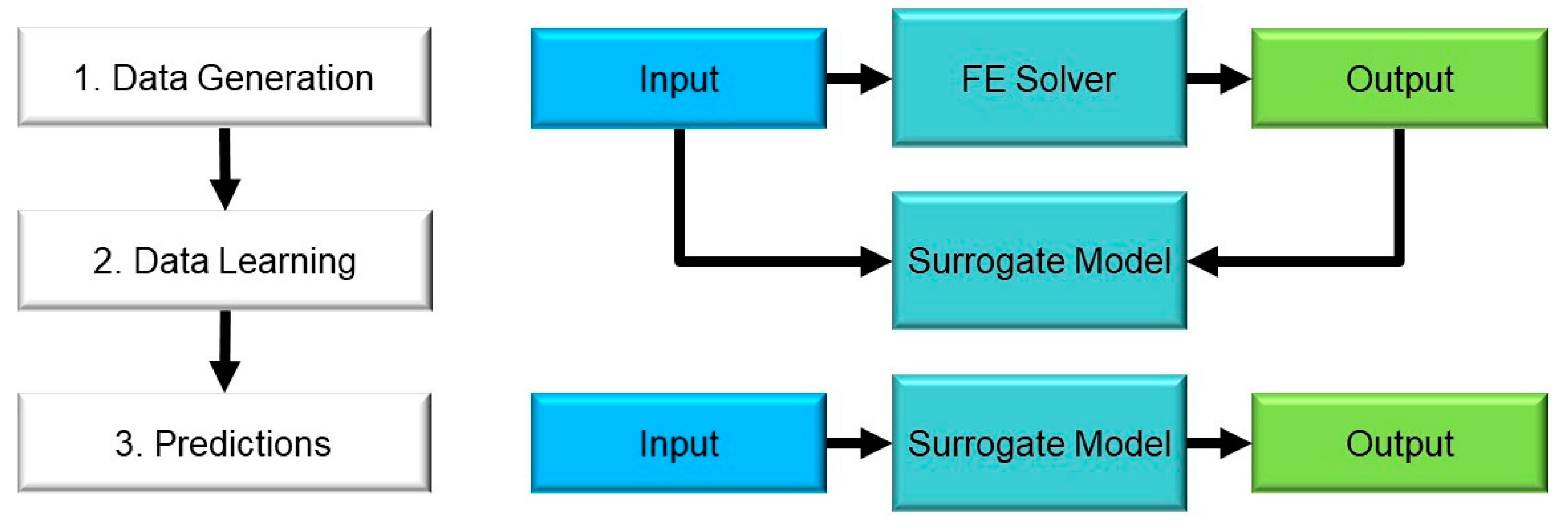
13]. In this regard, surrogate modes have recently been realized as a powerful analysis tool for different engineering fields [
14]. In general, the process of building and implementing surrogate models involves three primary steps (see
Figure 2):
Data generation. The modeler estimates the input, and then they generate the output via an FE solver;
Data learning. The correlation between the inputs and outputs is established via ML models;
Predictions. Given any set of inputs, the surrogate model can instantaneously compute the corresponding output.
Note that the term ”predictions” is commonly used in ML as the objective of many applications of ML is to predict future outcomes based on an analysis of past instances. It is important to remember that prediction means determining the output that an FE model would compute for the current application. Accordingly, a surrogate model could predict the output for combinations of input parameters that have yet to be modeled in the data learning stage. However, ML models generally perform poorly on data outside the learning process range [
12]. Hence, the surrogate model is usually limited to predicting outcomes based on parameters within the range assigned for the learning process (Stage 2 in
Figure 2). Ref. [
14] provided an excellent discussion of surrogate models and their use for rock mechanics problems. They argued that this tool has yet to be integrated into practice.
In this paper, we further investigated the coupling of ML and FE modeling for surrogate models. We demonstrated the application of a surrogate model for the analysis of two common rock slope stability problems: (1) determining the maximum depth of a vertical excavation and (2) determining the allowable angle of a slope with a fixed height. Through this process, various aspects of surrogate models were highlighted, including benefits and limitations. The GSI system was used for the analyses, and the impact of GSI range estimation on result distribution was investigated. The paper is hereinafter structured according to the three stages as shown in
Figure 2:
Section 2 and
Section 3 present the slope problems, including underlying assumptions for data generation;
Section 4 describes the learning process for setting and evaluating ML model performance;
Section 5 demonstrates the results from the execution of the surrogate models.
2. Vertical Excavation Problem Definition and Data Generation
Deep vertical top–down excavations in rock are needed for many applications, including basements, road cuts, underground train stations, and more. The rock mass strength generally dictates the degree of support required. Standard support measures, given from strong to weak rock masses, are as follows:
No support;
Occasional spot bolting and/or a thin layer of shotcrete;
Sequenced excavation and systematic application of shotcrete and bolting;
Installation of support before excavation, such as slurry walls.
The extent of support dramatically impacts the overall project budget [
15]. From economic and environmental perspectives, it is desirable to avoid an overly conservative design and minimize the extent of support. At the pre-feasibility stage, limited geological information is regularly available to the engineers. At this early stage, modeling the problem requires checking for a wide range of input parameters. As a project progresses to detailed design, efforts are made to minimize uncertainty and optimize design, and the amount of data collected will increase. Accordingly, the range of input parameters can be reduced.
The following problem is assumed for the current analysis: an excavation with varying depth, up to a maximum depth of 8 m, is required. The maximum permissible excavation depth with no support must be determined. An FE model is built accordingly, as shown in
Figure 3. The model is divided into nine stages: an initial geostatic stage and eight stages where increments of 1 m increase the depth. The model’s lower boundary is fully constrained, and roller constraints are assigned to both sides of the model to allow for vertical settlement. For such projects, it is important to account for loads that act near the excavation imposed by vehicles, future structures, etc. Therefore, a distributed load of 0.2 MN/m
2 is assigned at the top-level excavation boundary.
The rock mass is assumed to be weak and weathered, and the rock mass discontinuities are distributed equally in all directions. Thus, an equivalent isotropic and homogeneous continuum material is considered suitable for modeling purposes. Accordingly, an FE model with the generalized Hoek–Brown (HB) failure criterion could be used. The GSI rating, the ultimate compressive strength (UCS) of the intact rock, and other constants are used to compute the HB failure envelope for the rock mass. GSI is usually obtained from a visual examination and qualitative assessment of the rock mass structure and surface conditions of its discontinuities. Ref. [
16] cautioned against attempts to develop methods of GSI quantification because GSI is not a measurable physical quantity (it reflects qualitative geological conditions). Accordingly, it is wrong to assign exact values for GSI. Ref. [
17] showed that when using different quantification approaches, GSI values regularly fall within a range of ±10 of each other. Analyses conducted by [
18] showed a smaller range of ±7.5. Our models assumed a larger range of GSI ± 20 to simulate unknown conditions typical of a pre-feasibility study (
Table 1). For the ML learning stage, continuous GSI values were used for the purpose of building the proper numerical correlation. For the final stage of result interpretation, a narrow range of ±5 was used. It was assumed that a narrower range would be unacceptable given the nature of GSI as discussed.
In addition to peak strength parameters, residual parameters were defined for the GSI and intact rock constant m
i. Note that there are no accepted guidelines for determining residual strength parameters. For brittle rock masses, the residual strength is regularly considered to be lower than the peak strength, whereas for weak and ductile rock masses, there is no significant further weakening during the residual state. For the current study, we conservatively assumed weakening for the residual behavior of the rock mass. In addition to GSI, other input parameters were assigned a range of values.
Table 1 shows the minimum, mean, and maximum values for the varied input parameters. All models were loaded with gravitational forces according to a rock mass unit weight of 27 KN/m
3, and a lateral earth pressure at rest of 0.5.
For the slope problems discussed in this paper, the limit equilibrium method can be used for assessing slope stability factor of safety (FoS). In the limit equilibrium method, the slope is divided into slices and a series of iterative limit equilibrium equations are computed [
19]. The limit equilibrium method has the advantage of lesser computational costs. In contrast, FE solutions require significantly more computational resources, but in turn, have a number of advantages; they are capable of accounting for complex non-linear material behavior (e.g., elastoplastic post-peak behavior); FE models do not require an a priori assumptions regarding the shape of the slope failure surface; and FE solutions compute displacements, which in some cases can be useful for the purpose of monitoring and calibrating complex models.
The proposed methodology for surrogate models could be implemented with any solving method, and the optimal solving method depends on the nature of the specific case study. There are two primary benefits to using surrogate models. The first is computational efficiency, as ML models are capable of making rapid predictions. The second is rapid post-processing and visualization for a range of geometries and ground properties. While the first benefit may not apply to simplistic solving methods such as limit equilibrium, the second benefit holds for any solving method.
The commercial FE code RS2 was used for the 2D plane strain analysis [
20]. To cope with uncertainty, statistical tools and probabilistic analyses have been proposed and applied in geotechnical practice [
11]. The RS2 program consists of built-in probabilistic tools, including the Monte Carlo (MC) method. The MC method involves a rigorous iterative process where random generators create a variety of input parameters based on statistical distributions assigned by the user. In contrast, traditional deterministic analysis involves a single set of inputs. In current geotechnical practice, MC analysis is used predominantly for obtaining the statistical variation of results. The MC feature was used for this work to automate the modeling process. Accordingly, 800 FE models were automatically generated and solved. Note that prior to the automated process of model generation, it is recommended that a few models are solved and inspected thoroughly. Through this process, it is important to conduct a mesh sensitivity analysis, as well as making sure that results are sensible. Otherwise, the garbage-in–garbage-out phenomenon may occur and erroneous data would be passed into the surrogate model without detection. For the current models, six-noded triangular elements with a size of 0.7–1 m were used. Slope displacements with this mesh were found to be equal to models with elements ranging 0.3–0.6 m, thus proving that the selected size is satisfactory.
Elastoplastic FE models may fail to converge because of several possible reasons. However, if the models converge in the first stages, this rules out technical issues, such as mesh errors. The large deformations that develop during the non-converging stage indicate that the model behaves as desired, i.e., structural failure occurs due to increased excavation depth. Hence, the maximum excavation depth can be inferred according to the non-convergence stage. Considering the 1 m excavation increments (see
Figure 1), and owing to the initial geostatic stage, the maximum excavation depth is equal to the non-convergence stage minus two.
Figure 4 shows the distribution of modeling results according to maximum excavation depth. Although the input parameters were assigned a uniform distribution, the excavation depth results were non-uniform. This can be attributed primarily to nonlinear effects that skew results. In addition, the input parameters were generated randomly for each FE model, and therefore there is no guarantee that they should be evenly distributed. Nonetheless, obtaining a uniform distribution is unnecessary, as the objective is to have enough instances for the ML model to train on. In addition, it can be inferred from
Figure 4 that for the range of input parameters given in
Table 1, a clear decision cannot be made, as the permissible excavation depth varies from 2–8 m. This shows that a more precise input parameter estimate is needed to draw a meaningful conclusion.
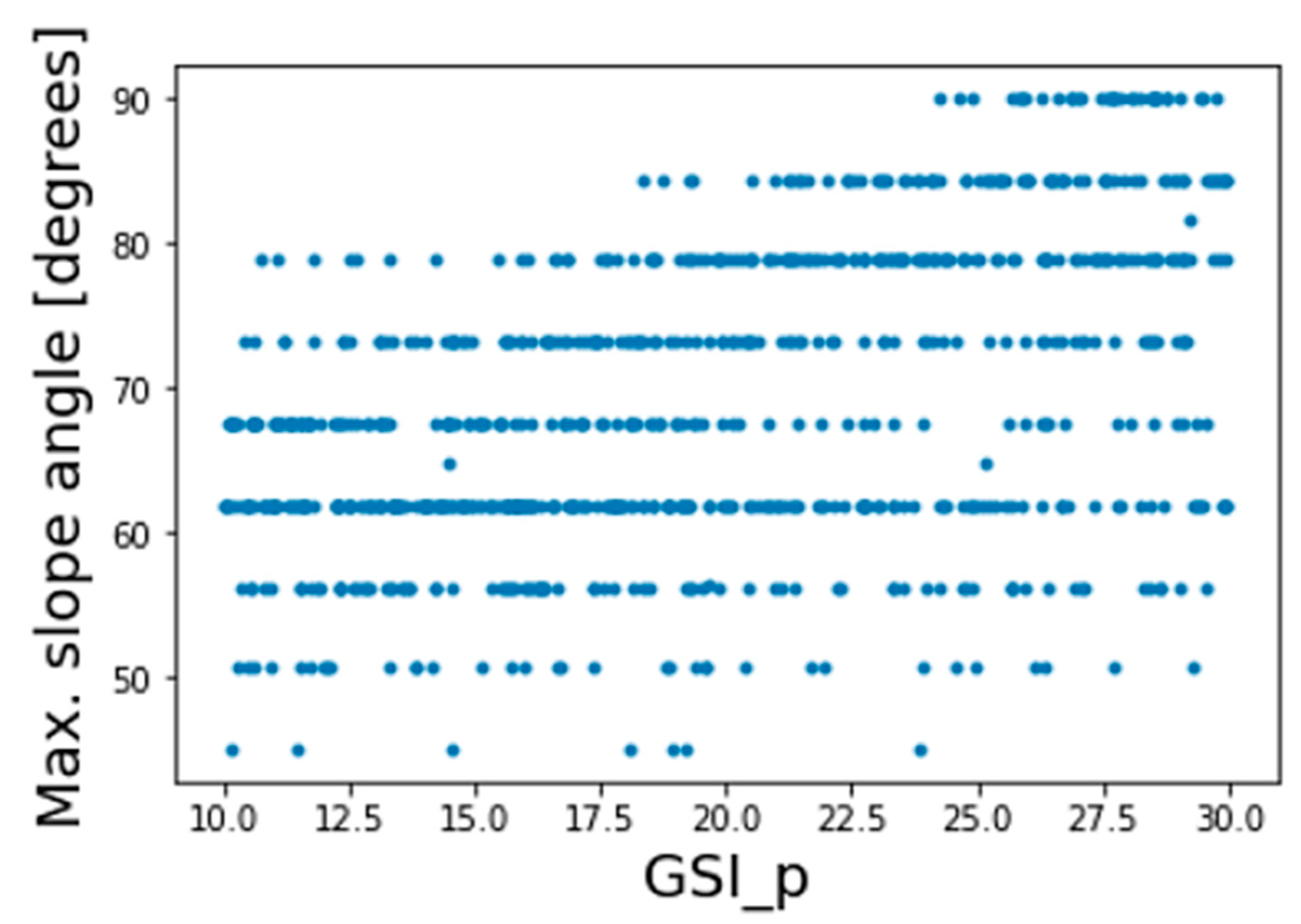
Figure 5 shows a plot of the peak GSI vs. maximum excavation depth for each of the 800 FE models. As can be noticed from this plot, the correlation between these two variables was not strong. Therefore, the peak GSI alone is a poor predictor of allowable excavation depth, and a more sophisticated analysis is needed for making predictions.
A Python script was created to collect the relevant data from the result files and organize them correctly for the subsequent ML analysis. Ultimately, two variables were created: a matrix where each row consists of the rock mass input parameters for each model and a column vector that consists of the corresponding maximum excavation depths. The ML model establishes a correlation between these two variables through an iterative process.
4. Learning Process
The learning process involves training an ML model on the data generated by the FE analysis and confirming that its performance is acceptable. In ML terminology, the learning process when the data consists of input features and a target is referred to as supervised training. In this case, the training process was performed on a subset of the data (referred to as the training set) of 600 FE models. The ML model performance was then assessed by making predictions on the remaining 200 models, referred to as the test set. The test–train split is essential to ML as it determines how well our model can generalize to unseen data [
21].
ML models can be generally divided into regression- and classification-type models. The first returns a continuous numerical prediction, and the second predicts a discrete class number. There is often no clear distinction between regression and classification modes, and both may be used [
22]. In the current study, the output values of maximum excavation depth were inferred from the model stage of non-convergence, and outputs were divided into discrete classes (see
Figure 2). Seemingly, a classification model is more suitable for this task. On the other hand, the data are not categorical but rather ordinal; therefore, it is possible that a regression ML model can perform better on this data.
Ultimately, it is best to repeat the train–test process for several types of ML models and compare their performance. For the current study, random forest (RF), support vector machines (SVM), and K-nearest neighbor (KNN) algorithms were compared, each for both classification and regression analysis. Explanations regarding how these models operate can be found in ML textbooks and are therefore not repeated here [
22]. The Scikit-Learn library was used to import the functions for the execution of the ML models.
Furtney at al. [
14] used artificial neural networks (ANNs) for their work with surrogate models for rock mechanics problems. While ANNs are powerful ML models that allow generalizing for highly complex data sets, they also require intensive fine-tuning of hyperparameters and a significant amount of data in the order of at least tens of thousands [
22]. Unlike empirical data, artificial data generated by numerical codes usually consist of low signal-to-noise ratios. It is therefore argued that for surrogate models, simpler ML models should be preferred over ANNs, so long that their performance is satisfactory. The open-source Python programming language was used for data pre-processing and ML applications.
There are different practices for fine-tuning models to achieve higher accuracy (e.g., cross-validation, hyperparameter tuning, and feature selection). Given the knowledge gaps in current geotechnical practice (see the discussion in [
7]), it would not be realistic to attain highly accurate predictions from numerical modeling. Therefore, knowing this limitation and distinguishing accuracy measured with ML performance with real-world predictive power is essential.
Several metrics are available for evaluating ML performance, including the coefficient of determination, mean square error, root-mean-square error (RMSE), and more. For the current analysis, the RMSE provides an intuitive understanding of the accuracy of the prediction of maximum excavation depth. For example, RMSE = 0.5 would indicate that, on average, the model’s predictions deviate by 0.5 m from the actual results. In general, RMSE is a performance metric suitable for regression models, whereas for classification models, other metrics are more appropriate (e.g., precision, recall, and accuracy). However, for the current problem, the categorical data can be treated as numerical data.
Figure 9 shows the scores of the RF, SVM, and KNN models. Each model is either denoted R for regression and marked in blue or C for classification models and marked in green. As seen in
Figure 8, the results were consistent for both the vertical excavation and slope problems. The RF model performed the best out of all three models. The apparent explanation for this is that the RF model is an ensemble method, i.e., it makes predictions based on several subsets of the data and selects based on the majority of predictions. Similar to the concept of the wisdom of the crowds in statistics, ensemble methods generally outperform regular ML models [
22].
When comparing the regression- and classification-type models, the former outperforms the latter for every type of model. This is attributed to the nature of classification models, which predict discrete values. As a result, on average, the error of wrong predictions is greater compared with regression models that can predict decimal values.
Figure 10 shows bar charts of the predicted vs. actual excavation results for ten randomly selected models from the RF regression (RFR) test set of the vertical excavation and slope problems. For the vertical excavation problem, most predictions missed by less than 0.5 m. For example, in the subset of models shown in
Figure 10a, for model #5 a depth of 4.1 m was predicted, vs. the actual result of 3 m; hence, the error is 1.1 m. It is advised to visually inspect all answers to detect whether the ML model is mis-predicting certain classes. This matter is of particular importance for the current type of engineering problems, where the primary concern of the engineers is identifying instability. The consequences of an erroneous prediction of stability can bring catastrophic results. In contrast, falsely predicting instability leads to over-conservative design, which is not desirable but less crucial. Currently, design procedures still need clear guidelines for the integration of surrogate models for practical purposes.
For classification-type models, results can be presented as a confusion matrix.
Figure 11 shows the confusion matrix for the results of the RF classification (RFC) model. The confusion matrix is organized so that its rows represent the true classes, and the columns represent predicted classes. The classes in this figure correspond to the eight possible excavation depths and slope angles, as shown in
Figure 3 and
Figure 6. In a perfect model, all non-zero values are located in the main diagonal. The results shown in the confusion matrix are normalized so that sum of all values in each row is equal to 1. The RFCs generally performed well, with mostly low values in the off-diagonal cells. Concerning the current type of problems, the confusion matrix allows for visualizing the types of errors: a conservative prediction of slope stability would skew the results left to the main diagonal, whereas an overly optimistic prediction would skew the results to the right. Therefore, compared with regression models, the confusion matrix in classification-type models provides an ideal means for gaining intuition regarding ML model conservatism.
The amount of required data is a fundamental question based on any data-scientific research project. Pre-hoc sample size determination is generally regarded as an unsolved challenge in the field of data science [
23]. Therefore, each problem requires determining sample size via post-hoc testing. To investigate the effect of the number of FE models on model performance, an iteration where a subset of the total number of FE models for training and testing was increased from 50 to 600 in increments of 10. For each iteration, the data were split into 75% for training and 25% for testing. This analysis was carried out for the RFR and RFC models, and its results are shown in
Figure 12. It can be seen that the RMSE diminished with an increasing number of models, as anticipated. For a small number of models, results were not reliable as the test set became very small and therefore not representative of model performance. From about 300–400 FE models, the marginal impact of adding models became negligible. Note that the results were not smooth, as ML algorithms use iterative and randomized methods for data fitting rather than closed-form solutions.
Feature importance in an ML model allows for determining each input’s relative impact on the model’s predictions. Feature importance can aid engineers in improving the performance of the ML model by removing the features that are less important (i.e., a form of feature selection) and allowing them to focus more on obtaining better quality data for the features that have been proven most important. The computational technique for feature importance was first published by [
24]. Compared with traditional sensitivity analyses that rely on linear relationships, feature importance has the advantage of accounting for non-linearities [
25]. The Sci-kit learn feature importance function was used to compute feature importance from the RFR model. The results of the feature importance analysis for the vertical excavation and inclined slope problems are shown in
Figure 13. The input parameters are listed according to the notation given in
Table 1. The results showed that the most important features are the peak GSI and UCS. This highlights the benefit of assessing parameter importance. For example, in a real-world scenario, this finding suggests that it would be more cost effective to invest in uniaxial tests to better quantify the UCS, rather than investing efforts in laboratory tests for the less-impactful parameters. However, there are some observable differences between the results of the two problems: the importance of the peak GSI relative to UCS is opposite for both problems, and the residual GSI is not negligible for the inclined slope problem. These differences reflect the limitation of feature importance, which is sensitive to the unique conditions of each problem. In other words, conclusions regarding feature importance should be made with caution.
Another important implication of feature critical analysis relates to back-analysis tasks. Real-world failures provide an essential opportunity for researchers to back-analyze the event and calibrate input parameters accordingly. Many scientific publications consider the general agreement between physical findings and modeling results as proof of successful back-analysis. However, several combinations of input parameters may yield similar results when there are multiple unknown input parameters. For the current example, feature importance showed that GSI and UCS are the most impactful predictors of slope failure. The UCS of the rock can be measured and assessed quite accurately, and, therefore, the GSI remains the single unknown that can be calibrated for back-analysis from real-world failure events.
5. Execution of the Surrogate Model
As geotechnical projects progress, more data become available, and better estimations of rock mass input parameters can be made. The RFR model, found to perform best in
Section 4, is used as a surrogate model for making predictions. As discussed in the previous section, feature importance showed that the peak GSI and UCS were the most impactful input parameters. The UCS of the intact rock can be measured through laboratory or in situ tests. GSI can be better estimated if more rock outcrops are made observable. Hence, it is reasonable to assume a narrower range of ±10 for these parameters in an advanced stage of a rock engineering project. Given a large excavation site, it is anticipated that the GSI and UCS values would vary.
To simulate this effect, two data sets were generated according to the values listed in
Table 2. The other parameters were kept constant according to the values listed in
Table 3. Each data set consists of 10,000 data points (i.e., sets of input parameters). Despite this large number of data points, predictions were made instantaneously, thus demonstrating the computational efficacy of the surrogate model.
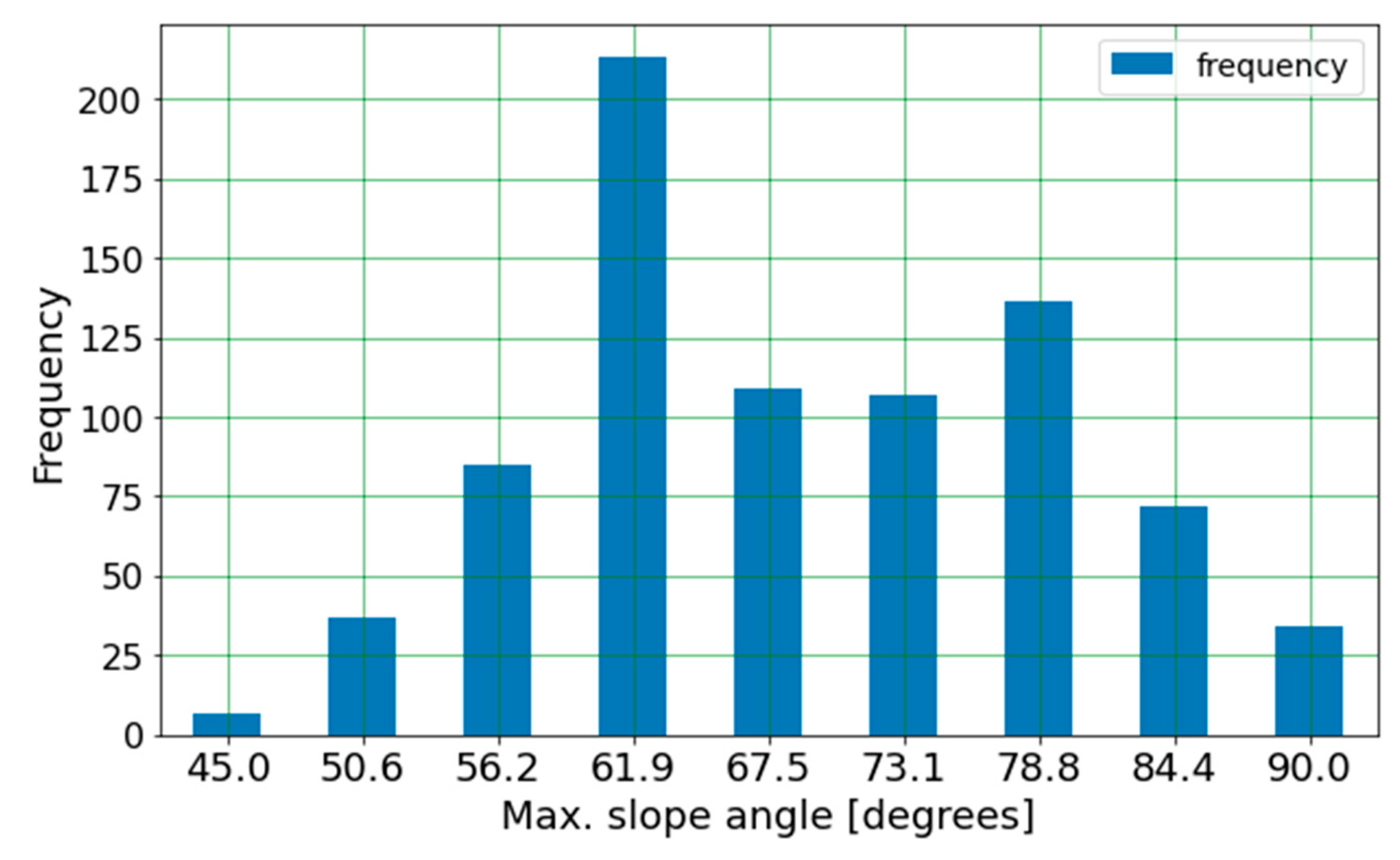
A histogram based on the predictions of the surrogate model is shown in
Figure 13. Note that the values from the regression model were rounded for the histogram. The effect of reducing the uncertainty can be acknowledged by comparing the histograms in
Figure 4 and
Figure 14. This comparison shows that the reduction from ±10 to ±20 for GSI and UCS significantly impacted the results. For the vertical excavation problem, most results indicated a maximum excavation depth of 3 m for data set #1. For data set #2, results distributed between 3 and 7 m. For the inclined slope problem, results ranged from 55° to 73° for data set #1 and 67° to 82° for data set #2. These findings highlight the benefit of surrogate models that allow for instantaneously examining the effect of gaining more data and narrowing the range of inputs. The current results showed that slope problems are nonlinear and therefore problem dependent.
From a practical perspective, it is important to bear in mind that the consequences in the face of a wrongful decision regarding slope stability can be catastrophic. Ultimately, the results of such analyses must be carefully considered alongside engineering judgment and experience. Nevertheless, given the current state of practice, where numerical simulations are used to aid the decision-making process of rock engineers, it is argued that surrogate models allow for more rigorous analysis without requiring high computational costs.
6. Conclusions and Limitations
Surrogate models involve three stages: (1) data generation, (2) data learning, and (3) predictions. The efficacy of using surrogate models for numerical analysis becomes apparent in stage 3, as the model needs to compute one simple matrix compared with an elastoplastic FE program that must solve large matrices over many iterations.
The integration of surrogate models into the process of numerical modeling for rock engineering problems was discussed through the analysis of two common practical problems, i.e., a vertical top–down excavation and an inclined slope. The GSI system was used for modeling, and the impact of the GSI range was investigated. The general methodology presented in this paper could be applied and further modified for the analysis of other geotechnical applications. For this reason, we made our data and code available online [
26].
The ML analysis (stage 2) for the given example showed that the regression models performed better than the classification models and that the RF model outperformed the SV machine and KNN models. The apparent explanation for this is that regression analysis allows for the prediction of continuous numerical values, whereas classification models are constrained to discrete values. For visualization, classification models can be presented via a confusion matrix. For engineering problems, the confusion matrix is useful for assessing the degree of ML model conservatism. It is further argued that more complex ML models such as ANNs are unnecessary for similar applications of surrogate models.
Feature importance provides insights regarding the relative impact of input parameters. Feature importance analysis for the data sets used for the vertical excavation and inclined slope problems showed that GSI and UCS were the most impactful input parameters. In contrast, the other parameters (additional HB parameters, elastic constants, residual strength parameters) had a minor influence on results.
Surrogate models allow for rapid analysis of the effect of input range on the distribution of results. Along with feature importance, this capability allows for exploring which parameters are most impactful in reducing uncertainty. In the data generation stage of the current analysis, the estimation of GSI and UCS was in the range of ±20. For this range, the results were found to distribute widely. The range was then reduced to ±10, and in turn, it was found that the range of results was significantly reduced.
Finally, it is essential to acknowledge the current limitations of research and practice in rock engineering. Firstly, surrogate models are based on FE analysis; therefore, ML analyses cannot eliminate the limitations of geotechnical analysis via FE modeling. Second, surrogate models are problem dependent; therefore, conclusions from one case study should not be applied to other cases without careful inspection.
Third, the integration of ML tools for rock engineering applications is still in its infancy. As a result, there are no guidelines for implementing ML in compliance with standard design procedures. For example, many local building codes commonly require calculating a slope FoS. In essence, the concept of FoS is influenced by engineering and statistical reasoning [
16]. How ML algorithms are executed implicitly impacts upon statistical aspects of FoS. More research is required to develop procedures for adequately integrating ML and surrogate models with established design procedures.


