Consistency Check of ITACAext, the Flatfile of the Italian Accelerometric Archive

Abstract

We present the results of a consistency check performed over a flatfile of accelerometric data extracted from the ITalian ACcelerometric Archive (ITACA), enriched with velocimetric records of events with magnitude M < 4.0. The flatfile, called ITACAext, includes 31,967 waveforms from 1709 shallow crustal earthquakes, in the magnitude range from 3.0 to 6.9, and occurred in the period of 1972–2019 in Italy. The consistency check is carried out by decomposing the residuals obtained from a reference ground motion model, for the ordinates of the 5% damped acceleration response spectra. The residual components are subsequently analyzed to identify a list of events, stations, and records that significantly deviate from the median trends predicted by the model. The results indicate that about 10% of events and stations are outliers, while only 1% of the waveforms present anomalous amplitudes. The asymmetrical azimuthal coverage of seismic stations around the epicenter is the most common issue that can affect the estimates of the repeatable event residual term. On the other hand, peculiarities in the site-response or wrong estimates of the soil parameters (i.e., the average shear-wave velocity in the first 30 m of the subsoil) are the main issues related to the repeatable station residuals. Finally, single records can show large residuals because of issues related to signal acquisition (e.g., multiple events, noisy records) or possible near-source effects (e.g., rupture directivity).

1. Introduction

The seismic waveforms and associated metadata of moderate-to-strong events are usually stored in structured archives and distributed via web-interfaces or web-services, which are widely used for engineering applications and seismological studies. These archives are generally supported by parametric tables, called flatfiles, created to disseminate intensity measures and associated metadata, widely used for the development of Ground Motion Models (GMMs) and other engineering applications (e.g., [1,2]).

The rapid growth of seismic monitoring networks in the last twenty years, and the availability of continuous real-time streaming from centralized repositories (e.g., EIDA; [3]), led to an exponential increase of seismic waveforms. This huge number of available records, which is expected to increase considerably over time, needs to be treated with automatic procedures or machine-learning techniques (e.g., [4,5,6,7]), aimed at supporting data-processing and data-quality control.

In this regard, one possible strategy is to perform some consistency check of the data stored in the flatfile, assessing how much each data point deviates from a median prediction model representative of the dataset. This analysis is useful to supply high-quality seismic data and metadata that allow providing robust estimates of the expected shaking, reducing the GMMs’ variability, and improving the Probabilistic Seismic Hazard Assessment (PSHA) (e.g., [8,9]).

One of the earliest proposals for identifying anomalous recording sites and events was formulated by Bindi et al. [10], in a study related to a subset of the Italian strong motion data, extracted by the ITACA database (ITalian ACcelerometric Archive; [11,12]), performing a residual analysis with respect to a reference ground motion model. Later, the increased number of earthquakes and recording sites, along with replacement of analog instruments with digital ones, allowed more robust estimations of systematic event and site residuals (e.g., [13,14]), in addition to the computation of the repeatable path and source effects in some densely sampled areas [15,16]. As a matter of fact, residual analysis has become increasingly important due to its ability to identify peculiar contributions in the observed ground motion, traceable to different effects, such as source, site, or instrumental disturbances (e.g., [17,18,19,20,21]), and exploited to systematically assess the quality of strong motion datasets.

Recently, residual analysis has been applied by Bindi et al. [22] to carry out a consistency check of the pan-European engineering strong motion (ESM) flatfile [1]. The authors identified those earthquakes, stations, and recordings showing the largest deviations from the median predictions of a GMM calibrated over the ESM flatfile data. A similar study was performed by Traversa et al. [23], applying the consistency check on the dataset derived from the Réseau Sismologique et géodésique Français (RESIF) network (https://www.resif.fr/en/presentation/interactive-map/; last accessed on 18 July 2022). In this case, the authors have considered the residual distributions obtained for the horizontal peak ground acceleration, PGA, and for the significant ground-motion duration, D_5–95. The former allowed recognizing atypical amplitudes, whereas the latter allowed identifying truncated signals or traces with noisy coda waves.

In this study, we present the results of a consistency check performed over ITACAext [24], a flatfile extracted by the waveforms collection of the version 3.2 of the ITalian ACcelerometric Archive (ITACA) [12], which is the most complete collection of accelerometric records of moderate-to-severe earthquakes (M > 3.0) which occurred in Italy since 1972, released with annual frequency to include a periodic revision as well as adding new waveforms and related metadata (e.g., considering updated seismic catalogs, last site characterization studies, new types of installation).

The consistency check on the ITACAext flatfile is based on the residual distributions obtained from the reference ground motion model for shallow crustal earthquakes in Italy (ITA18) [25], for the ordinates of the 5% damped acceleration response spectra. The computed residuals were analyzed to identify a list of events, stations, and records that significantly deviate from the median trends predicted by the model. To this aim, we set predefined amplitude thresholds for each residual component to identify peculiar features worthy of further investigations. The peculiarities identified by the consistency check are manually revised, providing illustrative cases and statistics on the possible causes.

2. Dataset

The investigated dataset is derived from the ITACAext flatfile [24]; https://itaca.mi.ingv.it/ItacaNet_32/#/products/itacaext_flatfile; last accessed on 18 July 2022], a parametric table created to disseminate intensity measures and metadata relative to the version 3.2 of ITACA [12]. To have a more robust estimation of the residual terms, ITACAext is also enriched with records not stored in the ITACA database. In particular, ITACAext includes some records acquired by the networks of the neighboring countries (such as France, Switzerland, Slovenia, Albania and Montenegro) and, for low seismicity or poorly monitored areas, it includes the velocimetric data of the National Seismic Network (RSN, http://cnt.rm.ingv.it/en/instruments/network/IV; last accessed on 18 July 2022), mainly for events with M < 4 available from the EIDA data stream [3]. ITACAext is formatted coherently with the ESM flatfile [1] and collects only waveforms manually processed following the procedure of Paolucci et al. [26]. Since all the collected signals are manually checked, the uncertainties on event and site metadata are expected to be the main cause of anomaly, such as in the case of earthquakes which occurred during seismic sequences or located offshore, and in the case of stations poorly characterized or equipped with analog instruments (e.g., [27,28]).

To perform the residual analysis, a subset of ITACAext is extracted within the range of validity of the ground motion model (ITA18) [25] adopted as reference in this study. The selection criteria are the following: (i) moment magnitude Mw (or local magnitude M_L if not available) larger than 3.0; (ii) epicentral distance lower than 220 km; (iii) exclusion of volcanic and subduction events (based on the SHARE seismogenic zonation) [29]; (iv) event shallower than 30 km; (v) exclusion of the borehole stations and of those installed on the building elevation floors; (vi) data up to 2019. We have not adopted any conversions from M_L to Mw because we observed that the uncertainty introduced by the different conversion laws would not lead to significant reductions in the total aleatory variability of the ground motion residuals.

The final dataset is the 98% of the starting ITACAext flatfile and consists of 31,967 recordings from 1709 shallow crustal earthquakes and 1716 stations. The overall magnitude-distance distribution (Figure 1a) covers a large range of magnitudes (3–6.9 Mw) and distances (0–220 km). The spatial distribution of the events across the Italian territory (Figure 1b) reflects the earthquake occurrence in the last 50 years, with the epicenters of the most relevant seismic sequences mainly located along the Apennine mountain chain, in the Po Plain sedimentary basin, and in the Eastern Alps. However, due to the particular tectonic and geodynamic setting of Italy, several events are also located offshore, along the coast, or abroad, mainly toward the Balkan peninsula. On the contrary, the collection of the recording sites in the study dataset allows for a denser spatial sampling and represents almost all the geologic environments in Italy (Figure 1c).

In the ITA18 model, the explanatory variable for the site term is the V_S,30 parameter (i.e., the average shear-wave velocity in the first 30 m of the subsoil), which is also adopted in the European seismic code (EC8) [30] for the soil category assignment. However, only about 25% of the Italian stations are characterized with a V_S,30 value computed from the measured shear-wave velocity (Vs) profile; for the other stations, this parameter is assessed from empirical correlations with the topographic slope [31], as well as from the EC8 soil category [30] inferred from surface geology (for each soil category, the average V_S,30 is considered). Figure 1d shows the availability of site information for the study dataset, confirming that, for the majority of the sites, surface geology and topographic slope are the only information available. In these cases, if these two proxies agree on the soil category assignment, we consider the V_S,30 obtained from topographic slope; otherwise we take the V_S,30 inferred from surface geology as this parameter is directly correlated with the type of deposit rather than on topographic slope, which may provide misleading information. For example, the station IT.CRV (locality of Carovigno), installed on the Apulian Carbonate Platform, is a case where despite the rock formation suggests V_S,30 > 800 m/s (i.e., soil category A) [30], the topographic slope is flat, indicating V_S,30 between 374 m/s and 421 m/s (i.e., soil category B) [30], depending on the resolution of the digital elevation model. The disagreement between these two proxies is related to the peculiar geological setting of the Carbonate Platform, where the stiffness of the stratigraphic deposit is not correlated to the increase in the topographic slope. In this case, the topographic proxy would provide an erroneous V_S,30 estimate. In some minor cases, the topographic slope is the only usable proxy, and when no site information is available (none in Figure 1d), the most common soil class B and V_S,30 = 580 m/s (360 m/s < V_S,30 < 800 m/s in Eurocode 8) [30] is assumed.

3. Method

3.1. Residual Analysis

For the residual analysis, we consider the partially non-ergodic ground motion model ITA18 [25], developed for the shallow crustal earthquakes in Italy. The ITA18 model is calibrated for RotD50 [32] of peak ground acceleration (PGA), peak ground velocity (PGV), and for 36 ordinates of acceleration response spectra (SA) at 5% damping in the 0.01 to 10 s period range. The calibration dataset includes 5607 records, relative to 146 earthquakes and 1657 stations. The validity range of the model is in the magnitude range between 4 and 8, with source-to-site distances in the range 0–200 km, and event depths shallower than 30 km. The predictor variables are the moment magnitude Mw, the source-to-site distance (either the closest distance to the rupture plane R_rup, or the Joyner–Boore distance, R_JB), and the V_S,30 as site parameter. The style of faulting, representing the classification of the events based on the rake angle [33], is also considered.

The total residuals ($R_{es}$) are computed on the ITACAext flatfile as the difference between the natural logarithm of observations and predictions. The residual components related to the events, stations, and to the random variability (see [34] for an excursus on terminology) are accomplished by decomposing the total residuals with the mixed-effect regression [35], according to the following expression:

$$R_{es}=a_0+{\mathsf{\delta }\mathrm{B}}_e+\mathsf{\delta }S2S_s+{\mathsf{\delta }\mathrm{W}}_{o,es},$$

(1)

where the subscripts e and s refer to event and station, respectively. a₀ is the average offset of the ITACAext residuals. ${\mathsf{\delta }\mathrm{B}}_e$ represents the between-event residual (event-term), which corresponds to the average misfit of recordings of the particular earthquake e with respect to the median ground-motion model (

Table 1. Residual components and corresponding standard deviations (modified after [34]).

Definition	Residual Component	Standard Deviation
Total	$R_{es}$	$\mathsf{\sigma }$
Between-event	${\mathsf{\delta }\mathrm{B}}_e$	$\mathsf{\tau }$
Site-to-site	$\mathsf{\delta }S2S_s$	${\mathsf{\Phi }}_{S2S}$
Event- and site-corrected	${\mathsf{\delta }\mathrm{W}}_{o,es}$	${\mathsf{\Phi }}_0$
Event- and site-corrected at single-site		${\mathsf{\Phi }}_{o,s}$

). $\mathsf{\delta }S2S_s$ is the site-term at the station s (Table 1), which quantifies the average misfit of recordings from one particular site, with respect to the median ground-motion predicted for the V_S,30 of the site. ${\mathsf{\delta }\mathrm{W}}_{o,es}$ is the remaining residual after site- and event-terms are subtracted from the total residual (Table 1).

The same decomposition of the residuals can be adopted for the corresponding standard deviations. The total standard deviation σ (Table 1), related to the total residual $R_{es}$, is computed as:

$$\mathsf{\sigma }=\sqrt{{\mathsf{\tau }}^2+{{\mathsf{\Phi }}_{S2S}}^2+{{\mathsf{\Phi }}_0}^2},$$

(2)

where τ and ${\mathsf{\Phi }}_{S2S}$ are the standard deviation of ${\mathsf{\delta }\mathrm{B}}_e$ and $\mathsf{\delta }S2S_s$ terms, respectively, and ${\mathsf{\Phi }}_0$ is the standard deviation of the event- and site-corrected residuals (Table 1). The remaining variability can be also estimated for an individual site s, ${\mathsf{\Phi }}_{o,s}$ (Table 1), as:

$${\mathsf{\Phi }}_{o,s}=\sqrt{\frac{{\sum }_{e=1}^{NEs}{{\mathsf{\delta }\mathrm{W}}_{o,es}}^2}{N{E}_s-1}},$$

(3)

where $N{E}_s$ is the number of events recorded at the site s.

First, we verify that the offset term (a₀), that quantifies the average deviation of the ITACAext dataset from ITA18 model is as small as possible. Figure 2 shows that the bias, normalized to the total standard deviation of the ITACAext residuals, is negative (within −15%) at all periods, with a peak of −35% around period T = 0.7 s. This offset is further investigated neglecting the a₀ term in Equation (1) and verifying the condition of zero-mean random variable at the two periods 0.01 s and 0.7 s, for each residual component (Figure 3), as a function of the corresponding explanatory variable (i.e., magnitude for ${\mathsf{\delta }\mathrm{B}}_e$, V_S,30 for $\mathsf{\delta }S2S_s$, and distance for ${\mathsf{\delta }\mathrm{W}}_{o,es}$). We can note that the scaling for small magnitude earthquakes is not perfectly captured by the ITA18 model (${\mathsf{\delta }\mathrm{B}}_e<0$ for M < 3.5; Figure 3a,b), and this is probably the cause of the overall negative values. Indeed, the single components are not affected by significant biases, except for the $\mathsf{\delta }S2S_s$ of soft sites (V_S,30 < 180 m/s, Figure 3c,d), and for the ${\mathsf{\delta }\mathrm{W}}_{o,es}$ of near-source records (distance < 5 km, Figure 3e,f), where very few data are available. These findings support the applicability of the ITA18 model to the ITACAext flatfile.

As expected, the residual analysis on the analyzed dataset provides higher variabilities than the ITA18 model (Figure 4). This is particularly evident for ${\mathsf{\delta }\mathrm{B}}_e$ and $\mathsf{\delta }S2S_s$ terms (Figure 4a,b), due to the large increment of events and stations in the ITACAext flatfile, whereas comparable values are observed for ${\mathsf{\delta }\mathrm{W}}_{o,es}$ residuals (Figure 4c).

3.2. Detection and Classification of Peculiar Features

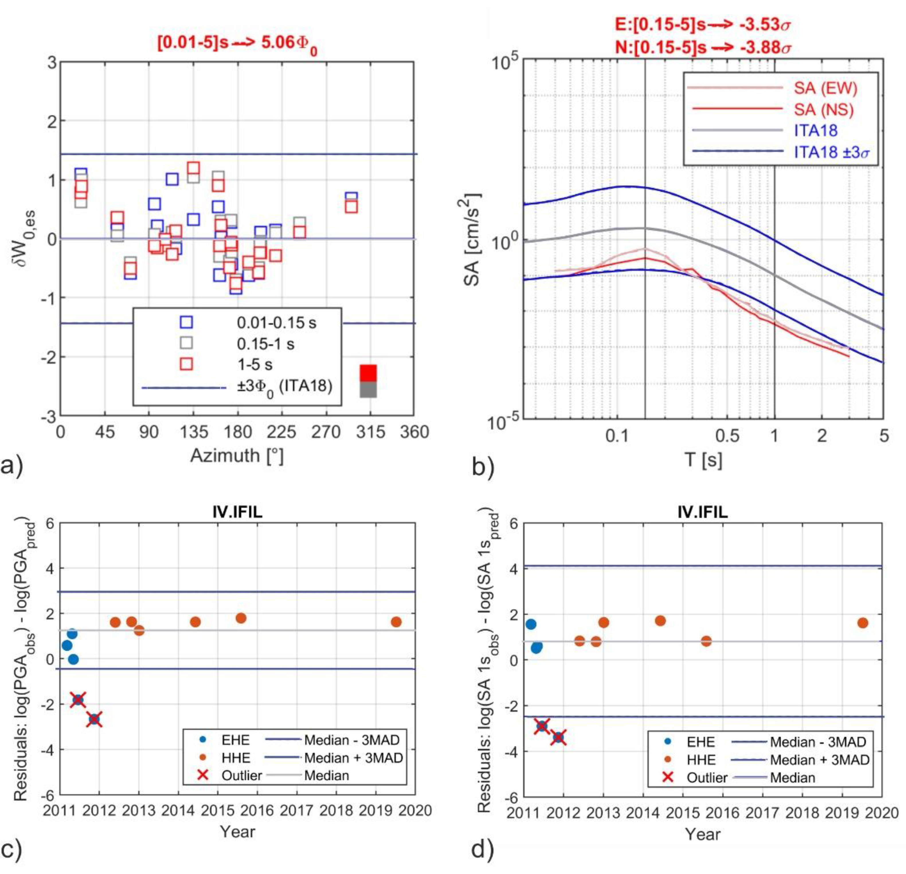
The workflow for the consistency check is reported in Figure 5. Starting from the ITACAext dataset (step 1 in Figure 5), the residuals analysis is performed to compute, for each event, station, and record, the between-event (${\mathsf{\delta }\mathrm{B}}_e$), the site-to-site ($\mathsf{\delta }S2S_s$), and the event-and-site-corrected (${\mathsf{\delta }\mathrm{W}}_{o,es}$) terms (step 2 in Figure 5). The residual components computed with less than 5 records are not considered, in agreement with the study of [36], which suggested a criterion of 3 to 8 recordings per event to have stable results.

The outliers in the ITACAext flatfile are identified based on some predefined thresholds (step 3 in Figure 5). Bindi et al. [22] adopted, as limit value, 3 times the standard deviations of the GMM residual components (i.e., 3τ, 3${\mathsf{\Phi }}_{S2S}$ and 3${\mathsf{\Phi }}_0$); this is in agreement with the current practice in PSHA, in which the ground motion distribution is truncated at a fixed number (ε = 3) of the logarithmic standard deviation (e.g., [8]). A more restrictive threshold is selected in Traversa et al. [23], where all records with $\left|{\mathsf{\delta }\mathrm{W}}_{o,es}\right|$ > 2${\mathsf{\Phi }}_0$ are manually inspected.

Considering these previous studies, and after some tests performed on the study dataset, we conservatively adopt a threshold of 2${\mathsf{\tau }}_{ITA18}$ and 2${\mathsf{\Phi }}_{S2S, ITA18}$ for ${\mathsf{\delta }\mathrm{B}}_e$ and $\mathsf{\delta }S2S_s$, respectively (step 3 in Figure 5), and a threshold of 3${\mathsf{\Phi }}_0$, _ITA18 for ${\mathsf{\delta }\mathrm{W}}_{o,es}$. The residual components, normalized w.r.t. the corresponding standard deviation, are computed in three ranges of periods (i.e., 0.01–0.15 s, 0.15–1 s, 1–5 s) to investigate the ground motion at short-, intermediate- and long- periods. When the standardized residuals exceed the corresponding threshold in at least one of the considered period intervals, a warning is raised.

Once detected, the outliers are classified in order to investigate the possible causes (step 4 in Figure 5). Outliers for ${\mathsf{\delta }\mathrm{B}}_e$, $\mathsf{\delta }S2S_s$ and ${\mathsf{\delta }\mathrm{W}}_{o,es}$ may indicate peculiarities related to the source of the event (e.g., stress drop), the site response of the station (e.g., basin effects), and the source-site effects (e.g., directivity), respectively, besides possible errors in the corresponding metadata, or instrument malfunctions. For example, if a record is characterized by total residuals $R_{es}>3{\mathsf{\sigma }}_{ITA18}$ and, eventually, high aleatory variability at single-site (${\mathsf{\Phi }}_{o,s}>1$), issues on the acquisition parameters, such as gain, full scale or channel sensitivity may be occurred. All anomalous cases are presented in the supplementary materials.

The events, sites and records of the ITACAext flatfile that exceed the residual thresholds are manually reviewed to identify the corresponding features and to provide overall statistics on the relative occurrences. In the following, some illustrative cases of the warnings distribution on the ITACAext flatfile are presented.

4. Results

4.1. Illustrative Cases

Figure 6 shows two cases relative to the outliers on the event term (event IDs refer to the ITACA database).

The first event EMSC-20120609_0000005, located in Northeastern Italy with M_W 4.0, presents ${\mathsf{\delta }\mathrm{B}}_e$ residuals that exceed on average 3.46 ${\mathsf{\tau }}_{ITA18}$ in the range 0.01–5 s (Figure 6a, black curve). This event was recorded by 51 seismic stations, the majority located SouthWest of the earthquake epicenter. As a matter of fact, this event occurred during the time span of the 2012 Emilia seismic sequence (e.g., [37]), when several temporary seismic stations were installed in the Po Plain area to improve the detection performance of permanent monitoring systems ([38]; Figure 6b). As for many other events of the ITACAext flatfile, this anomaly may be related to a low azimuthal coverage that does not capture all path effects and spatial anisotropies in the ground-motion distribution, causing a trade-off between event, and path effects in ${\mathsf{\delta }\mathrm{B}}_e$ estimation that could limit its physical interpretation.

The second event IT-2012-0032, located in the Po Plain area (Northern Italy) with M_W 5.5, has negative residuals that are on average −2.9 ${\mathsf{\tau }}_{ITA18}$ in the range 1–5 s (Figure 6a, gray curve). This event is part of the 2012 Emilia seismic sequence and occurred in a time window characterized by several earthquakes that often overlap on the corresponding records, causing anomalies on ${\mathsf{\delta }\mathrm{B}}_e$ residuals estimation. In this case, 20 s before the IT-2012-0032 event, a smaller event (ID: IT-2012-0076), with a magnitude M_W 4.9, occurred. The overlap of these two events depends on the relative position between the recording stations and the earthquake epicenters. Figure 6c shows the location of the IT-2012-0032 and IT-2012-0076 epicenters, along with the spatial distribution of recording stations. As an example, we show the recording of the IV.T0819 station, about 7 km from the epicenters, where the two events can be easily trimmed on the raw traces (Figure 6d), and the recording of the IV.T0820 station, at about 50 km from the epicenters, where the two events tend to overlap (Figure 6e). Moreover, the late-arriving long-period surface waves can significantly increase the duration of ground shaking, causing overlaps along their propagation path, in particular in the Po Plain, where many factors strongly favor the generation of surface waves in the radiation path from the source (e.g., [37,39,40]).

The illustrative cases for the $\mathsf{\delta }S2S_s$ peculiarities are reported in Figure 7. At the IT.BCN site (locality of Buccino in Southern Italy), the prediction model overestimates the ground motion at low frequency. The site residual is negative and is on average −2.75 ${\mathsf{\Phi }}_{S2S}$ in the range 0.01–5 s (Figure 7a), due to a probable erroneous site classification (soil category D: V_S,30 < 180 m/s; [30]). In absence of in-situ measurements, the V_S,30 parameter was inferred from surface geology at large scale. However, the 1:100.000 geology map indicates that the target seismic station is at the boundary between a coarse sedimentary deposit and an outcropping limestone formation. As a matter of fact, the flat Horizontal-to-Vertical (H/V) spectral ratio from ambient-noise (Figure 7b) suggests that the station should be classified in soil category A [30], for which the ground-motion model would provide lower spectral accelerations in agreement with the observations. Moreover, a soil category A is also indicated by the topographic proxy, being the site located on a mountain slope (Figure 7c,d). Based on this evidence, we prefer to use the proxy from topographic slope for the soil classification of the IT.BCN station.

Another representative example of the $\mathsf{\delta }S2S_s$ peculiarities in the ITACAext flatfile is the IV.SACR seismic station (locality of S. Croce del Sannio in Southern Italy), classified in soil category A (V_S,30 > 800 m/s; [30]) from surface geology, with $\mathsf{\delta }S2S_s$ residuals that are on average −2.81 ${\mathsf{\Phi }}_{S2S}$ between 0.01–0.15 s (Figure 7a). This site is classified as reference site, i.e., sites in soil category A (V_S,30 > 800 m/s; [30]) free of any amplification phenomena (Figure 7b) according to the study of Lanzano et al. [20]. Indeed, compared to ground motion predictions at generic rock sites in soil category A, the high frequency median ground-motion predicted for reference rock sites is significantly reduced (up to 40% at T = 0.1 s, [20]). In addition, the IV.SACR site has a high-frequency attenuation parameter k₀ of 0.0449 s, which is particularly high among the reference rock sites in Italy that have an average k₀ around 0.025 s [41].

Finally, the site IT.MLC (locality of Malcesine in Northern Italy), classified in soil category B (360 < V_S,30 < 800; [30]) based on geophysical surveys, shows a particular $\mathsf{\delta }S2S_s$ residual that exceed 2.15 ${\mathsf{\Phi }}_{S2S}$ between 0.01–0.15 s. This feature may be related to specific site effects between 3 and 10 Hz (i.e., 0.1–0.2 s), as indicated by the microtremor H/V spectral ratio in Figure 7b, and to the reflections from the Moho discontinuity that enhance PGA and short period spectral ordinates at distance larger than 70 km [15,42,43].

The illustrative cases for the peculiar ${\mathsf{\delta }\mathrm{W}}_{o,es}$ residuals are reported in Figure 8. Figure 8a shows the ${\mathsf{\delta }\mathrm{W}}_{o,es}$ residuals as a function of azimuth, for all recordings of the event EMSC-20160903_0000009 (M_W 4.2). The residuals, computed from the RotD50 [32] of the horizontal components, are averaged in the short (0.01–0.15 s), intermediate (0.15–1 s), and long (1–5 s) period ranges. This visualization allows recognizing anomalies in the spatial distribution of the ground motion. These anomalies may be ascribed to rupture directivity effects, i.e., the focusing of the radiated seismic wave energy in specific directions linked to the rupture propagation along the fault [44,45,46,47], which may induce peculiar residuals on the ${\mathsf{\delta }\mathrm{W}}_{o,es}$ component. In this case (Figure 8a), we observe high ground-motions in the direction of 315–360° North, particularly in the short-period range between 0.01–0.15 s. This observation is in agreement with the findings of Colavitti et al. [48], which report directivity effects also for small-to-moderate events in different frequency ranges. In particular, for the event EMSC-20160903_0000009 considered in Figure 8a, Colavitti et al. [48] indicate a rupture directivity at 332° North, between 1–25 Hz. This effect can be also appreciated on the spatial distribution of the PGA amplitudes in Figure 8b.

Besides source effects, the anomalies on the ${\mathsf{\delta }\mathrm{W}}_{o,es}$ residuals can be also related to low quality data that escaped manual control. For example, Figure 8c shows the ${\mathsf{\delta }\mathrm{W}}_{o,es}$ residuals of the event EMSC-20160824_0000192, located in Central Italy, with M_W 3.9. In this case, the accelerometric recordings of the IT.VNF1 seismic station, at a distance of 161 km from the epicenter, present anomalous ${\mathsf{\delta }\mathrm{W}}_{o,es}$ residuals that exceeds 4.54${\mathsf{\Phi }}_0$, ITA18 in the short period range (0.01–0.15 s). The accelerometric time history of this record is reported in Figure 8d.

Finally, for the peculiar features related to the acquisition parameters, an illustrative case is reported in Figure 9a, with the ${\mathsf{\delta }\mathrm{W}}_{o,es}$ residuals of the event IT-2011-0056, located in the Tyrrhenian sea, with M_L 3.5. Among the corresponding records, the IV.IFIL velocimetric station, located on the Filicudi Island (Aeolian Islands) at 37.8 km from the epicenter, presents anomalous ${\mathsf{\delta }\mathrm{W}}_{o,es}$ residuals that exceed 5.06${\mathsf{\Phi }}_0$ in all the 0.01–5 s period range (filled squares in Figure 9a). This record shows also anomalous amplitudes on $R_{es}$ residuals that are lower than 3.53σ for the N-S component and lower than 3.88σ for the E-W component, in all the 0.01–5 s period range (Figure 9b). The evolution in time of the total residuals for PGA (Figure 9c) and Sa 1 s (Figure 9d) at the IV.IFIL seismic station shows a systematic bias between the observed and predicted ground-motion levels, on both broadband (HH) and medium band (EH) velocimetric sensors. Indeed, the total residuals are centered around positive median values between 0 and 2 for both PGA (Figure 9c) and Sa 1s (Figure 9d). However, there are some records that do not follow this median trend. These records are referred to as outliers (Figure 9 c,d) and are detected when total residuals exceed more than three scaled Median Absolute Deviations, MAD (for a random variable vector A made up of N scalar observations, the median absolute deviation, MAD, is defined as: $MAD=median\left(A_i-\mathrm{median}\left(A\right)\right)$ for i = 1,2, …, N), away from the median. They indicate that the EH sensor of the IV.IFIL seismic station could have some issues related to the signal acquisition (e.g., gain, full scale, channel sensitivity), shortly before being replaced with the HH sensor, after a period of no data transmission (http://www.orfeus-eu.org/data/eida/quality; last accessed on 18 July 2022).

The outliers with these features are reported in

Table 2. Anomaly due to a possible issue with the acquisition parameters (format: network code.station code_event ID).

Records
FR.ESCA_EMSC-20140912_0000057
FR.ESCA_EMSC-20150411_0000019
FR.ESCA_EMSC-20151106_0000016
FR.ESCA_EMSC-20160623_0000055
FR.ESCA_EMSC-20160730_0000088
FR.REVF_IT-2012-0043
FR.REVF_IT-2012-0045
FR.REVF_IT-2012-0047
FR.REVF_IT-2012-0079
FR.REVF_IT-2012-0087
IV.IFIL_IT-2011-0056
IV.IFIL_IT-2011-0097
NI.DST2_EMSC-20190922_0000076
NI.DST2_EMSC-20191001_0000131

, such as the accelerometric station of the North-East Italy Broadband Network (NI.DST2) that presented anomalous recordings in 2019, besides two French stations near the Italian border (FR.ESCA and FR.REVF) that were already reported in [23] for the anomalous high PGA values between 2012 and 2016.

4.2. Percentage of Outliers

The statistics computed on the anomalies detected on the ITACAext flatfile (Tables S1–S3 of the electronic supplement) are reported in Figure 10.

Figure 10a shows that 14% of the events on the ITACAext flatfile (252 out of 1709) presents peculiarities on the ${\mathsf{\delta }\mathrm{B}}_e$ residuals. Most of these (~ ⅔) are characterized by an uneven distribution of stations that may affect the computation of the ${\mathsf{\delta }\mathrm{B}}_e$. A further 12% of the identified events occurred during seismic sequences, when multiple overlapping events often affect the recorded ground-motion, if not properly separated. Just a small amount of events (8%) may be related to other causes that need to be further investigated.

As regards the sites, Figure 10b shows that 11% (195 out of 1716) presents anomalies on the $\mathsf{\delta }S2S_s$ residuals. Among these, a 61% of the sites is characterized by peculiar site-effects not properly modeled by the target ground motion model (e.g., site amplifications at specific frequencies or systematic amplification/deamplification in the high-frequency range) and the remaining 39% is affected by a possible incorrect attribution of the soil category or V_S,30 value.

Finally, as regards the records of the ITACAext flatfile, Figure 10c shows that just 1% (272 out of 31967) presents peculiarities on the ${\mathsf{\delta }\mathrm{W}}_{o,es}$ residuals. Most of these (47%) are related to source effects (e.g., near-source or directivity effects) that may induce high ground-motions. Among the remaining records, a 38% is related to low-quality data that escaped manual control (e.g., one component is twice the other, noisy records, presence of spurious spikes) and a 15% is related to other still unexplained causes.

5. Conclusions

In this study, we presented the results of a consistency check over the ITACAext flatfile [24], based on the computation of the residuals obtained from a reference GMM, for the ordinates of the 5% damped acceleration response spectra. The total residuals (log difference between observations and predictions) are then further decomposed in between-event, site-to-site, and event-and-station-corrected residuals by applying a mixed-effect regression [35]. When a residual exceeds a predefined threshold, we detect a peculiarity that is subsequently analyzed in order to identify the possible causes. The outliers are manually reviewed to provide overall statistics on the occurrences of each peculiarity.

The study dataset includes data up to 2019, consisting of 31,967 recordings from 1709 shallow crustal earthquakes and 1716 stations. The results of the consistency check indicate that low percentages of events (14%), sites (11%) and records (1%) are outliers, confirming the high quality of the data and metadata included in the ITACA database, from which the ITACAext flatfile is extracted. The list of outliers is reported in the electronic appendices for the events (Table S1), sites (Table S2), and records (Table S3).

Overall, the residual-based consistency check of the strong and weak motion flatfiles can be a powerful tool, since it allows:

• identifying erroneous event (e.g., magnitude estimates, localization), site (e.g., soil category, V_S,30), and record (e.g., wrong acquisition parameters) metadata;
• discarding remaining low quality data;
• identifying physical effects not modeled by the reference GMM (e.g., peculiar site effects, rupture directivity).

The proposed method is effective in detecting possible anomalies in large flatfiles of seismic records, and it appears particularly useful for: (i) supporting automatic processing of seismic waveforms by identifying low-quality data; (ii) supporting the maintenance of seismic networks by detecting problems on the acquisition parameters; or (iii) guiding decisions on site characterization studies in case of anomalous site responses. For future developments, we plan to apply the same consistency check on a flatfile extracted from the ESM database [49], which stores and distributes the records in the European-Mediterranean regions and the Middle East.

References

1. Lanzano, G.; Sgobba, S.; Luzi, L.; Puglia, R.; Pacor, F.; Felicetta, C.; D’Amico, M.; Cotton, F.; Bindi, D. The pan-European Engineering Strong Motion (ESM) flatfile: Compilation criteria and data statistics. Bull. Earthq. Eng. 2019, 17, 561–582. [Google Scholar] [CrossRef]
2. Lanzano, G.; Sgobba, S.; Luzi, L.; Pacor, F.; Puglia, R.; Felicetta, C.; D’Amico, M. The pan-European engineering strong motion (ESM) flatfile: Comparison with NGA-West2 database. BGTA-Boll. Geofis. Teor. Appl. 2020, 61, 343–356. [Google Scholar] [CrossRef]
3. Strollo, A.; Cambaz, D.; Clinton, J.; Danecek, P.; Evangelidis, C.P.; Marmureanu, A.; Ottemöller, L.; Pedersen, H.; Sleeman, R.; Stammler, K.; et al. EIDA: The European integrated data archive and service infrastructure within ORFEUS. Seismol. Res. Lett. 2021, 92, 1788–1795. [Google Scholar] [CrossRef]
4. Hearne, M.; Thompson, E.M.; Schovanec, H.; Rekoske, J.; Aagaard, B.T.; Worden, C.B. USGS automated ground motion processing software. USGS Softw. Release 2019. [Google Scholar] [CrossRef]
5. Aur, K.A.; Bobeck, J.; Alberti, A.; Kay, P. Pycheron: A Python-Based Seismic Waveform Data Quality Control Software Package. Seismol. Res. Lett. 2021, 92, 3165–3178. [Google Scholar] [CrossRef]
6. Zaccarelli, R.; Bindi, D.; Strollo, A. Anomaly detection in seismic data–metadata using simple machine-learning models. Seismol. Res. Lett. 2021, 92, 2627–2639. [Google Scholar] [CrossRef]
7. Massa, M.; Scafidi, D.; Mascandola, C.; Lorenzetti, A. Introducing ISMDq—A Web Portal for Real-Time Quality Monitoring of Italian Strong-Motion Data. Seismol. Res. Lett. 2022, 93, 241–256. [Google Scholar] [CrossRef]
8. Bommer, J.J.; Abrahamson, N.A. Why do modern probabilistic seismic hazard analyses lead to increased hazard estimates? Bull. Seismol. Soc. Am. 2006, 96, 1967–1977. [Google Scholar] [CrossRef]
9. Rodriguez-Marek, A.; Rathje, E.M.; Bommer, J.J.; Scherbaum, F.; Stafford, P.J. Application of single-station sigma and site-response characterization in a probabilistic seismic-hazard analysis for a new nuclear site. Bull. Seismol. Soc. Am. 2014, 104, 1601–1619. [Google Scholar] [CrossRef]
10. Bindi, D.; Luzi, L.; Pacor, F. Interevent and Interstation Variability Computed for the Italian Accelerometric Archive (ITACA). Bull. Seismol. Soc. Am. 2009, 99, 4. [Google Scholar] [CrossRef]
11. Luzi, L.; Hailemikael, S.; Bindi, D.; Pacor, F.; Mele, F.; Sabetta, F. ITACA (ITalian ACcelerometric Archive): A web portal for the dissemination of the Italian strong motion data. Seismol. Res. Lett. 2008, 79, 716–722. [Google Scholar] [CrossRef]
12. Russo, E.; Felicetta, C.; D’Amico, M.; Sgobba, S.; Lanzano, G.; Mascandola, C.; Pacor, F.; Luzi, L. Italian Accelerometric Archive v3.2; Istituto Nazionale di Geofisica e Vulcanologia, Dipartimento della Protezione Civile Nazionale: Milano, Italy, 2022. [Google Scholar] [CrossRef]
13. Rodriguez-Marek, A.; Montalva, G.A.; Cotton, F.; Bonilla, F. Analysis of single-station standard deviation using the KiK-net data. Bull. Seismol. Soc. Am. 2011, 101, 1242–1258. [Google Scholar] [CrossRef]
14. Luzi, L.; Bindi, D.; Puglia, R.; Pacor, F.; Oth, A. Single-station sigma for Italian strong-motion stations. Bull. Seismol. Soc. Am. 2014, 104, 467–483. [Google Scholar] [CrossRef]
15. Lanzano, G.; D’Amico, M.; Felicetta, C.; Luzi, L.; Puglia, R. Update of the single-station sigma analysis for the Italian strong-motion stations. Bull. Earth. Eng. 2017, 15, 2411–2428. [Google Scholar] [CrossRef]
16. Sgobba, S.; Lanzano, G.; Pacor, F. Empirical nonergodic shaking scenarios based on spatial correlation models: An application to central Italy. Earthq. Eng. Struct. Dyn. 2021, 50, 60–80. [Google Scholar] [CrossRef]
17. Bindi, D.; Luzi, L.; Pacor, F.; Paolucci, R. Identification of accelerometric stations in ITACA with distinctive features in their seismic response. Bull. Earth. Eng. 2011, 9, 1921–1939. [Google Scholar] [CrossRef]
18. Pilz, M.; Cotton, F. Does the one-dimensional assumption hold for site response analysis? A study of seismic site responses and implication for ground motion assessment using KiK-Net strong-motion data. Earthq. Spectra 2019, 35, 883–905. [Google Scholar] [CrossRef]
19. Pilz, M.; Cotton, F.; Kotha, S.R. Data-driven and machine learning identification of seismic reference stations in Europe. Geoph. Journ. Intern. 2020, 222, 861–873. [Google Scholar] [CrossRef]
20. Lanzano, G.; Felicetta, C.; Pacor, F.; Spallarossa, D.; Traversa, P. Methodology to identify the reference rock sites in regions of medium-to-high seismicity: An application in Central Italy. Geoph. Journ. Intern. 2020, 222, 2053–2067. [Google Scholar] [CrossRef]
21. Kotha, S.R.; Weatherill, G.; Bindi, D.; Cotton, F. A regionally-adaptable ground-motion model for shallow crustal earthquakes in Europe. Bull. Earth. Eng. 2020, 18, 4091–4125. [Google Scholar] [CrossRef]
22. Bindi, D.; Kotha, S.R.; Weatherill, G.; Lanzano, G.; Luzi, L.; Cotton, F. The pan-European engineering strong motion (ESM) flatfile: Consistency check via residual analysis. Bull. Earth. Eng. 2019, 17, 583–602. [Google Scholar] [CrossRef]
23. Traversa, P.; Maufroy, E.; Hollender, F.; Perron, V.; Bremaud, V.; Shible, H.; Drouet, S.; Guéguen, P.; Langlais, M.; Wolyniec, D.; et al. RESIF RAP and RLBP dataset of earthquake ground motion in mainland France. Seismol. Res. Lett. 2020, 91, 2409–2424. [Google Scholar] [CrossRef]
24. Brunelli, G.; Lanzano, G.; D’Amico, M.C.; Felicetta, C.; Luzi, L.; Mascandola, C.; Pacor, F.; Russo, E.; Sgobba, S. ITACAext Flatfile [Data Set]; Istituto Nazionale di Geofisica e Vulcanologia: Milano, Italy, 2022. [Google Scholar] [CrossRef]
25. Lanzano, G.; Luzi, L.; Pacor, F.; Felicetta, C.; Puglia, R.; Sgobba, S.; D’Amico, M. A Revised Ground-Motion Prediction Model for Shallow Crustal Earthquakes in Italy. Bull. Seismol. Soc. Am. 2019, 109, 525–540. [Google Scholar] [CrossRef]
26. Paolucci, R.; Pacor, F.; Puglia, R.; Ameri, G.; Cauzzi, C.; Massa, M. Record processing in ITACA, the new Italian strong-motion database. In Earthquake Data in Engineering Seismology; Springer: Dordrecht, The Netherlands, 2011; pp. 99–113. [Google Scholar]
27. Trifunac, M.D.; Lee, V.W. A note on the accuracy of computed ground displacements from strong-motion accelerograms. Bull. Seismol. Soc. Am. 1974, 64, 1209–1219. [Google Scholar] [CrossRef]
28. Graizer, V. Strong motion recordings and residual displacements: What are we actually recording in strong motion seismology? Seismol. Res. Lett. 2010, 81, 635–639. [Google Scholar] [CrossRef]
29. Woessner, J.; Danciu, L.; Giardini, D.; Crowley, H.; Cotton, F.; Grünthal, G.; Valensise, G.; Arvidsson, R.; Basili, R.; Demircioglu, M.N.; et al. The 2013 European seismic hazard model: Key components and results. Bull. Earth. Eng. 2015, 13, 3553–3596. [Google Scholar] [CrossRef]
30. CEN; Eurocode. 8—Design of STRUCTURES for Earthquake Resistance—Part 1: General Rules, Seismic Actions and Rules for Building; Br. Stand. Institute: London, UK, 2004. [Google Scholar]
31. Wald, D.J.; Allen, T.I. Topographic slope as a proxy for seismic site conditions and amplification. Bull. Seismol. Soc. Am. 2007, 97, 1379–1395. [Google Scholar] [CrossRef]
32. Boore, D.M. Orientation-Independent, Nongeometric-Mean Measures of Seismic Intensity from Two Horizontal Components of Motion. Bull. Seismol. Soc. Am. 2010, 100, 1830–1835. [Google Scholar] [CrossRef] [Green Version]
33. Boore, D.M.; Atkinson, G.M. Ground-motion prediction equations for the average horizontal component of PGA, PGV, and 5%-damped PSA at spectral periods between 0.01 s and 10.0 s. Earthq. Spectra 2008, 24, 99–138. [Google Scholar] [CrossRef]
34. Al-Atik, L.; Abrahamson, N.A.; Bommer, J.J.; Scherbaum, F.; Cotton, F.; Kuehn, N. The variability of ground-motion prediction models and its components. Seismol. Res. Lett. 2010, 81, 794–801. [Google Scholar] [CrossRef]
35. Bates, D.; Mächler, M.; Bolker, B.; Walker, S. Fitting linear mixed-effects models using lme4. arXiv 2014, arXiv:1406.5823. [Google Scholar]
36. Ktenidou, O.J.; Roumelioti, Z.; Abrahamson, N.; Cotton, F.; Pitilakis, K.; Hollender, F. Understanding single-station ground motion variability and uncertainty (sigma): Lessons learnt from EUROSEISTEST. Bull. Earth. Eng. 2018, 16, 2311–2336. [Google Scholar] [CrossRef]
37. Luzi, L.; Pacor, F.; Ameri, G.; Puglia, R.; Burrato, P.; Massa, M.; Augliera, P.; Franceschina, G.; Lovati, S.; Castro, R. Overview on the strong-motion data recorded during the May–June 2012 Emilia seismic sequence. Seismol. Res. Lett. 2013, 84, 629–644. [Google Scholar] [CrossRef]
38. Moretti, M.; Abruzzese, L.; Zeid, N.A.; Augliera, P.; Azzara, R.A.; Barnaba, C.; Benedetti, L.; Bono, A.; Bordoni, P.; Boxberger, T.; et al. Rapid response to the earthquake emergency of May 2012 in the Po Plain, northern Italy. Ann. Geoph. 2012, 55, 4. [Google Scholar] [CrossRef]
39. Abraham, J.R.; Lai, C.G.; Papageorgiou, A. Basin-effects observed during the 2012 Emilia earthquake sequence in Northern Italy. Soil Dyn. Earthq. Engin. 2015, 78, 230–242. [Google Scholar] [CrossRef]
40. Paolucci, R.; Mazzieri, I.; Smerzini, C. Anatomy of strong ground motion: Near-source records and three-dimensional physics-based numerical simulations of the Mw 6.0 2012 May 29 Po Plain earthquake, Italy. Geophl. J. Int. 2015, 203, 2001–2020. [Google Scholar] [CrossRef]
41. Lanzano, G.; Felicetta, C.; Pacor, F.; Spallarossa, D.; Traversa, P. Generic-To-Reference Rock Scaling Factors for Seismic Ground Motion in Italy. Bull. Seismol. Soc. Am. 2022, 112, 1583–1606. [Google Scholar] [CrossRef]
42. Bragato, P.L.; Sugan, M.; Augliera, P.; Massa, M.; Vuan, A.; Saraò, A. Moho reflection effects in the Po Plain (northern Italy) observed from instrumental and intensity data. Bull. Seismol. Soc. Am. 2011, 101, 2142–2152. [Google Scholar] [CrossRef]
43. Lanzano, G.; D’Amico, M.; Felicetta, C.; Puglia, R.; Luzi, L.; Pacor, F.; Bindi, D. Ground-motion prediction equations for region-specific probabilistic seismic-hazard analysis. Bull. Seismol. Soc. Am. 2016, 106, 73–92. [Google Scholar] [CrossRef]
44. Anderson, J.G. Earthquake Seismology-physical processes that control strong ground motion. In Treatise on Geophysics, 2nd ed.; Elsevier: Amsterdam, The Netherlands, 2007. [Google Scholar]
45. Ben-Menahem, A. Radiation of seismic surface waves from finite moving sources. Bull. Seismol. Soc. Am. 1961, 51, 401–435. [Google Scholar] [CrossRef]
46. Boatwright, J. The persistence of directivity in small earthquakes. Bull. Seismol. Soc. Am. 2007, 97, 1850–1861. [Google Scholar] [CrossRef]
47. Joyner, W. Directivity for non-uniform ruptures. Bull. Seismol. Soc. Am. 1991, 81, 1391–1395. [Google Scholar] [CrossRef]
48. Colavitti, L.; Lanzano, G.; Sgobba, S.; Pacor, F.; Gallovič, F. Empirical Evidence of Frequency-Dependent Directivity Effects from Small-to-Moderate Normal Fault Earthquakes in Central Italy. Solid Earth. 2022, 127, e2021JB023498. [Google Scholar] [CrossRef]
49. Luzi, L.; Lanzano, G.; Felicetta, C.; D’Amico, M.C.; Russo, E.; Sgobba, S.; Pacor, F.; ORFEUS Working Group 5. Engineering Strong Motion Database (ESM) (Version 2.0); Istituto Nazionale di Geofisica e Vulcanologia (INGV): Milano, Italy, 2020. [Google Scholar] [CrossRef]
Figure 1. (a) Magnitude (M)—Distance (REPI) distribution grouped by hypocentral depth (h); (b) geographic distribution of earthquake epicenters with magnitude (M); (c) geographic distribution of seismic stations (IV: network code of the National Seismic Network (RSN, http://cnt.rm.ingv.it/en/instruments/network/IV; last accessed on 18 July 2022); IT: network code of the National Accelerometric Network (RAN, http://ran.protezionecivile.it/IT/index.php; last accessed on 18 July 2022); (d) availability of site information.
Geosciences 12 00334 g001
Figure 2. Offset term a0, normalized for the total standard deviation of the ITACAext residuals.
Geosciences 12 00334 g002
Figure 3. Residual components computed on the ITACAext flatfile, considering the ITA18 ground-motion model [25] as reference. Between-event residuals δ B e at T = 0.01 s (a) and T = 0.7 s (b). Between-station residuals δ S 2 S s   at T = 0.01 s (c) and T = 0.7 s (d). Event- and station-corrected residuals δ W o , e s at T = 0.01 s (e) and T = 0.7 s (f). Gray dots: all data; white dots: mean values.
Geosciences 12 00334 g003
Figure 4. ITA18 versus ITACAext flatfile variability. (a) Between-event standard deviation, τ; (b) site-to-site standard deviation, Φ S 2 S , and (c) event- and site-corrected standard deviation, Φ 0 .
Geosciences 12 00334 g004
Figure 5. Workflow for the consistency check of the ITACAext flatfile.
Geosciences 12 00334 g005
Figure 6. (a) examples of peculiar δ B e residuals; (b) spatial distribution of the epicenter (star) and recordings (triangles) for the event EMSC-20120609_0000005. The colors represent the Peak Ground Acceleration (PGA) at each station. The black box indicates the epicentral area of the 2012 Emilia seismic sequence. (c) Spatial distribution of the epicenters related to the IT-2012-0032 and IT-2012-0076 events. The recording stations highlighted in red are those whose accelerometric time series are reported in panels (d) (raw traces) and (e) (processed traces). The red box indicates the IT-2012-0076 event in the pre-signal noise of IT-2012-0032, whereas the blue lines delimitates the trimmed waveforms.
Geosciences 12 00334 g006
Figure 7. (a) examples of peculiar δ S 2 S s residuals in different shades of gray, along with the threshold of 2 Φ S 2 S in blue lines. (b) Microtremor H/V spectral ratios, where the solid lines indicate the average values and the gray shadows the corresponding standard deviations. (c) Installation site of the IT.BCN seismic station (red box), with a zoom in panel (d).
Geosciences 12 00334 g007
Figure 8. (a) example of peculiar δ W o , e s residuals due to rupture directivity of the event EMSC-20160903_0000009, and (b) spatial distribution of the corresponding PGA values. (c) Example of peculiar δ W o , e s residual due to a bad quality recording of the event EMSC-20160824_0000192 (filled squares highlight the anomalous values); and (d) accelerometric time history of the anomalous record highlighted in panel (c).
Geosciences 12 00334 g008
Figure 9. Example of peculiar δ W o , e s residual due to a possible issue with the acquisition parameters. (a) δ W o , e s residuals of the event IT-2011-0056. The filled squares indicate the anomalous δ W o , e s values at the IV.IFIL seismic station. (b) R e s residuals relative to the recording of the IT-2011-0056 event at the IV.IFIL seismic station. (c) Evolution in time of the total residuals of the PGA on both the broadband (HH) and medium band (EH) velocimetric sensors at the IV.IFIL seismic station. (d) Same for Sa 1s.
Geosciences 12 00334 g009
Figure 10. Statistics computed after manual revision of the peculiar events (a), sites (b) and records (c).
Geosciences 12 00334 g010