Article

An Approach for the Automatic Characterization of Underwater Dunes in Fluviomarine Context

Département des Sciences Géomatiques, Université Laval, Québec City, QC G1V 0A6, Canada
*
Author to whom correspondence should be addressed.
Geosciences 2022, 12(2), 89; https://doi.org/10.3390/geosciences12020089
Submission received: 20 January 2022 / Revised: 11 February 2022 / Accepted: 13 February 2022 / Published: 16 February 2022

Abstract

:
The identification of underwater landforms represents an important role in the study of the seafloor morphology. In this context, the segmentation and characterization of underwater dunes allow a better understanding of the dynamism of the seafloor, since the formation of these structures is directly related to environmental conditions, such as current, tide, grain size, etc. In addition, it helps to ensure safe navigation, especially in the context of navigation channels requiring periodic maintenance. This paper proposes a novel method to automatically characterize the underwater dunes. Its originality relies on the extraction of morphological descriptors not only related to the dune itself, but also to the fields where the dunes are located. Furthermore, the proposed approach involves the entire surface of the dunes, rather than profiles or group of pixels as generally found in previous works. Considering the surface modelled by a digital bathymetric model (DBM), the salient features of the dunes (i.e., crest line, stoss trough, and lee trough) are first identified using a geomorphometric analysis of the DBM. The individual dunes are built by matching the crest lines with their respective troughs according to an object-oriented approach. Then, a series of morphological descriptors, selected through a literature review, are computed by taking advantage of the dune salient features, surface representation, and spatial distribution in the fields where they are located. The validation of the proposed method has been conducted using more than 1200 dunes in the fluvio-marine context of the Northern Traverse of the Saint Lawrence River.

1. Introduction

The occurrence of sedimentary structures on the seafloor surface is related to the interaction between relatively strong or large-scale sustained flows and the sediments present on the water column. Different structures can be associated with distinct hydrodynamical factors, such as the flow velocity, the grain size of sediment transported by the flow, the meteorological conditions, tidal regime, etc. An underwater dune is a sedimentary structure present on the seafloor of shallow marine environments, estuaries, deltas, and river channels. These sedimentary structures can have a high migration rate on the seafloor based on the environmental dynamism [1,2,3,4,5,6,7]. Therefore, the segmentation and characterization of the underwater dunes have multiple purposes. In the context of navigation, the identification of these structures is particularly useful to ensure safe navigation. In addition, it improves efficiency and effectiveness of maintenance activities, such as dredging [8,9,10]. The identification of these sedimentary structures provides realistic seafloor representation to hydrodynamic simulation models involved in flood risk assessment in coastal areas. The recognition of dunes on the seafloor can also be used in the study of the sand banks erosion [11] and in the changes of the morpho-sedimentary dynamics of the seafloor [12]. They also contribute to the temporal monitoring of marine habitats [13].
High-resolution surveys using multibeam echosounders (MBES) allow the production of seafloor digital surfaces, such as digital bathymetric models (DBMs), from which the dunes can be identified. Dune identification and characterization by different experts, such as geomorphologists and hydrographers, is still mostly performed visually from DBMs [14]. However, this task is time-consuming, subjective, and less suited to large volumes of data. Hence, different computer-aided approaches have been proposed to segment underwater dunes from DBMs to alleviate the subjectivity and burden of this task. Generally, these approaches consider a geomorphometric analysis of the seafloor in order to identify the dunes or their salient features. For example, the authors of [15] proposed a method which identifies and segments the dunes in three steps. The first step performs a geomorphon classification [16] of the seafloor, extracting the crest line of the dunes. The second step identifies the dune itself, aggregating specific geomorphon classes. Then, the third step identifies the lee and stoss sides of the dunes. This step also computes dune metrics from equidistant vertical profiles along the dune. The authors of [17] state that a dune can be identified from its salient features, i.e., its crest line and its troughs. Hence, they proposed an approach where crest lines and troughs are first detected as lines from the DBM using mathematical morphology and image processing after an initial geomorphometric analysis of the seafloor. The DBM is segmented into dunes in a second step considering an object-based approach, matching each crest line with its respective troughs. The result is the dune objects segmented in a raster file.
Even if dunes can be automatically segmented, their characterization is mostly accomplished manually. As a result, it is often subjective and inaccurate. Such characterization can also be performed through the computation of morphological descriptors using the profiles of the dunes. An example is the computation of the angles of the sloping sides of the dunes. They are calculated based on the profile of the dune between the line connecting the crest line and the troughs of the dune [15,18]. Since we consider the dune as an object identified on the seafloor by its salient features, it can be characterized by different morphological descriptors related to its full surface rather series of sampled profiles. In addition, the identification of dunes present within the same field helps to correlate their characteristics and, by the same token, to characterize the field. In this paper, we propose an automatic method to (1) extract morphological descriptors towards a comprehensive characterization of the underwater dunes and (2) compute morphological descriptors of dune fields, moving towards a comprehensive characterization of underwater dunes and the fields where they are located. To our knowledge, such a method is currently missing in the literature. Ultimately, the availability of such morphological descriptors will allow a better understanding of the dunes and their development, which represent crucial knowledge for hydrospatial data users [19].
The paper is organized into four sections. The first section is a state of the art on the dune formation process, its definition as a sedimentary structure, and the dune morphological descriptors described in the literature. The second section presents the proposed method dedicated to the automatic extraction of morphological descriptors related to dune objects and dunes fields. The third section presents the experimental results related to the application of the method in the Northern Traverse of the Saint Lawrence River. This study zone was chosen since this navigation channel is a well-surveyed area given the presence of dunes fields on the seafloor. The fourth section discusses the experimental results and the method learning outcomes on the studied area, before concluding and providing perspectives for future research addressing the study and analysis of underwater dunes.

2. Underwater Dunes

In this section, we present the underwater dune formation process as well as the morphological descriptors related to this sedimentary structure.

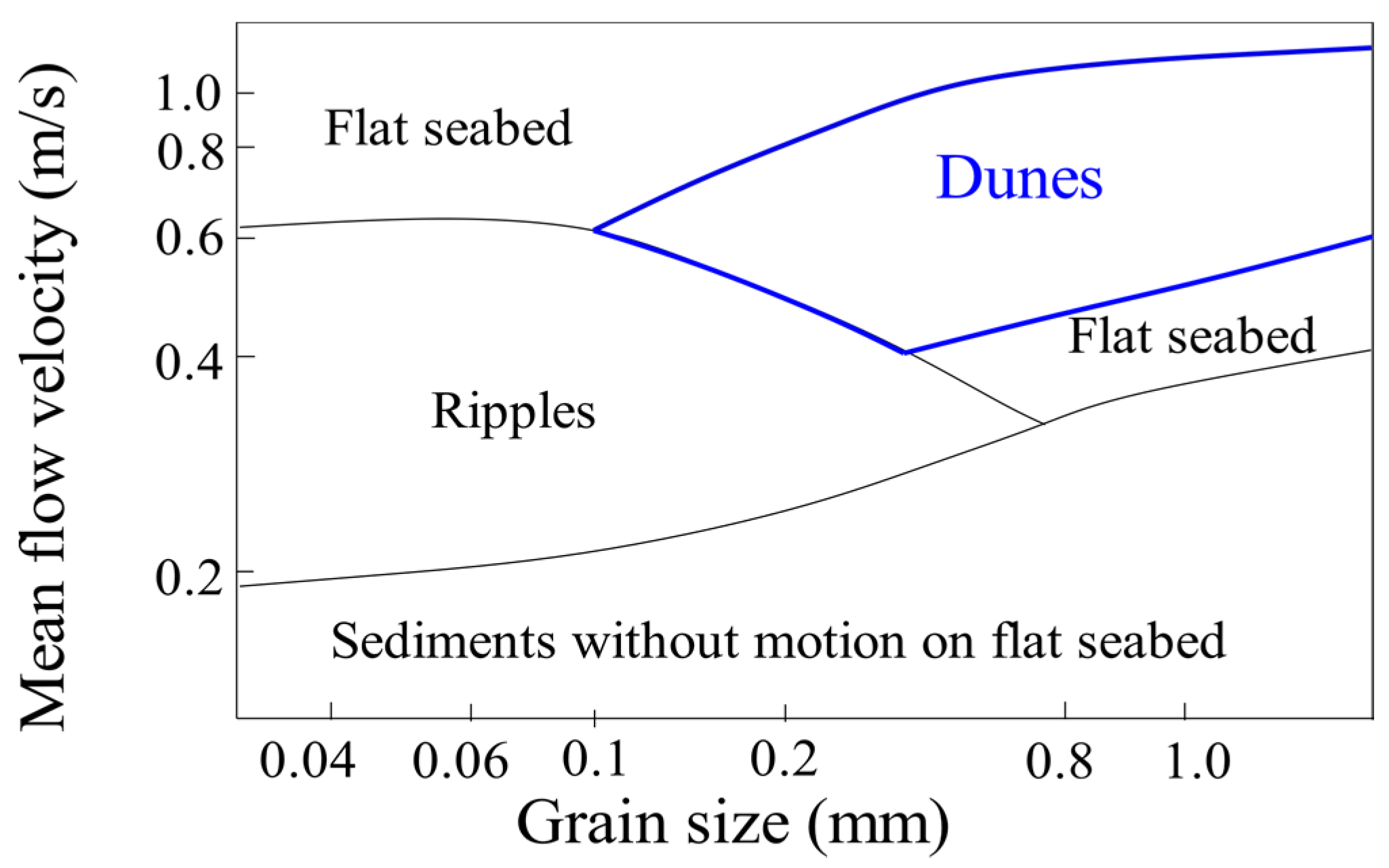
2.1. Formation of the Underwater Dunes

Underwater dunes (henceforward dunes) are the result of sediment transportation through time by a flow. In fact, there is a correlation between the grain size of the sediments and the flow velocity in the resulting sedimentary structure formed on the seafloor (Figure 1). The dune migration and shape are correlated to its nature and to hydrodynamic factors [4,20,21,22,23].
Figure 1 shows that dunes are formed with grain size ranging from gravel to fine sand (i.e., grain size greater than 0.1 mm up to more than 1.0 mm). Dunes are limited in finer sediments, such as silt or very fine sand [4]. According to the dunes classification proposed by the author of [24], dunes have a height ranging from 0.075 m up to 5 m and spacing from 0.6 m to more than 100 m. The height and spacing of dunes usually increase with the flow velocity [8,25]. These and other morphological descriptors shall be further described in the paper. Dunes have a gentle slope facing the current and a steep slope in its direction. A crest line separates these two slope sides, which are bounded by its troughs. The gentle slope is defined as the stoss side and is bounded by the crest line and the stoss trough. The steep slope of the dune is defined as the lee side and is bounded by the crest line and the lee trough. The lee side of the dune indicates the migration direction of this structure. The stoss and lee sides of the dunes are adjacent to each other [1,17,23,26]. Figure 2 illustrates a representation of this sedimentary structure and its related features.
Due to the complex flow dynamics, smaller sedimentary structures, such as ripples, can superimpose on underwater dunes [3,24]. As highlighted by the authors of [1], the presence of superimposed structures on the dunes varies on the grain size sediment and the dimensions of the dune. The superimposed structures can be from a few centimeters high up to a few meters, yielding asymmetric structures. These structures are formed on the dune stoss trough, and they migrate to the crest line of the dune, avalanching on the lee side [26]. In the proposed research, the available data and related 1 m resolution DBM do not have a resolution fine enough to analyze smaller structures that can superimpose on dunes, such as ripples. Thus, they will not be considered in the rest of the paper. Dunes can be found on the seafloor as isolated structures or adjacent to each other. The troughs of an isolated dune bound this structure with the stoss and lee troughs, which are associated with only one crest line. In the context of adjacent dunes, the troughs can be associated with more than one crest line. Indeed, the lee trough of a dune is the stoss trough of the following dune in the field. Figure 3 illustrates the difference between an isolated dune and adjacent dunes.

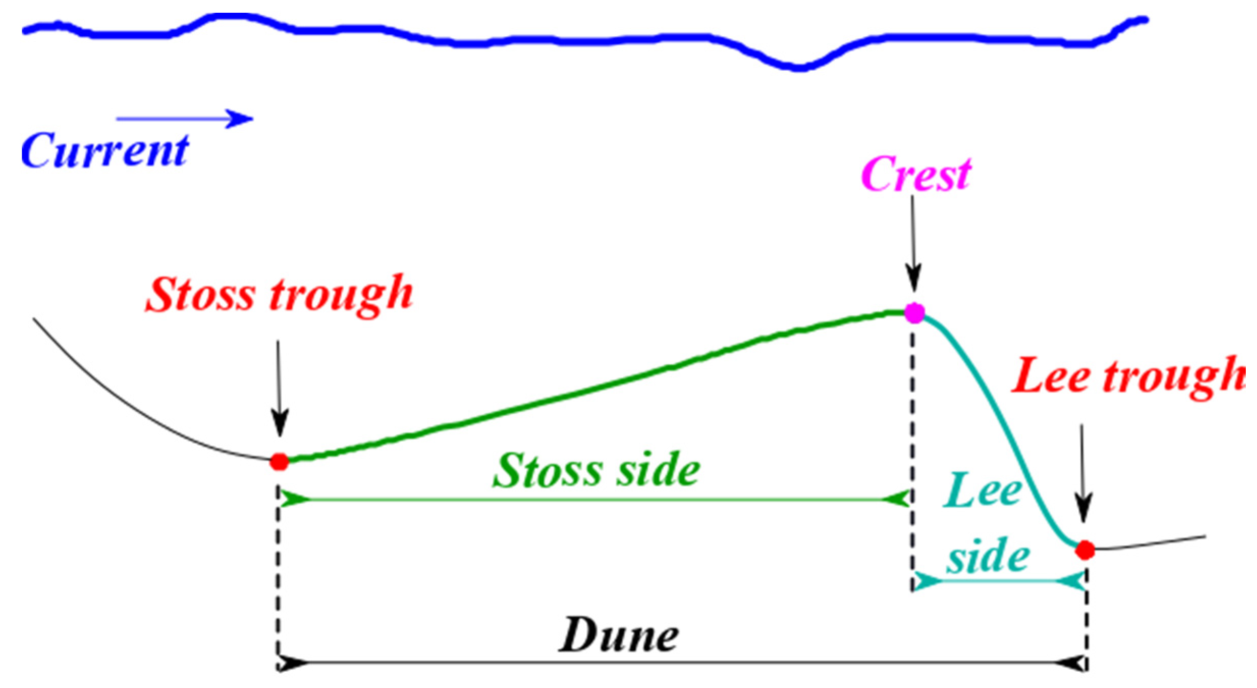
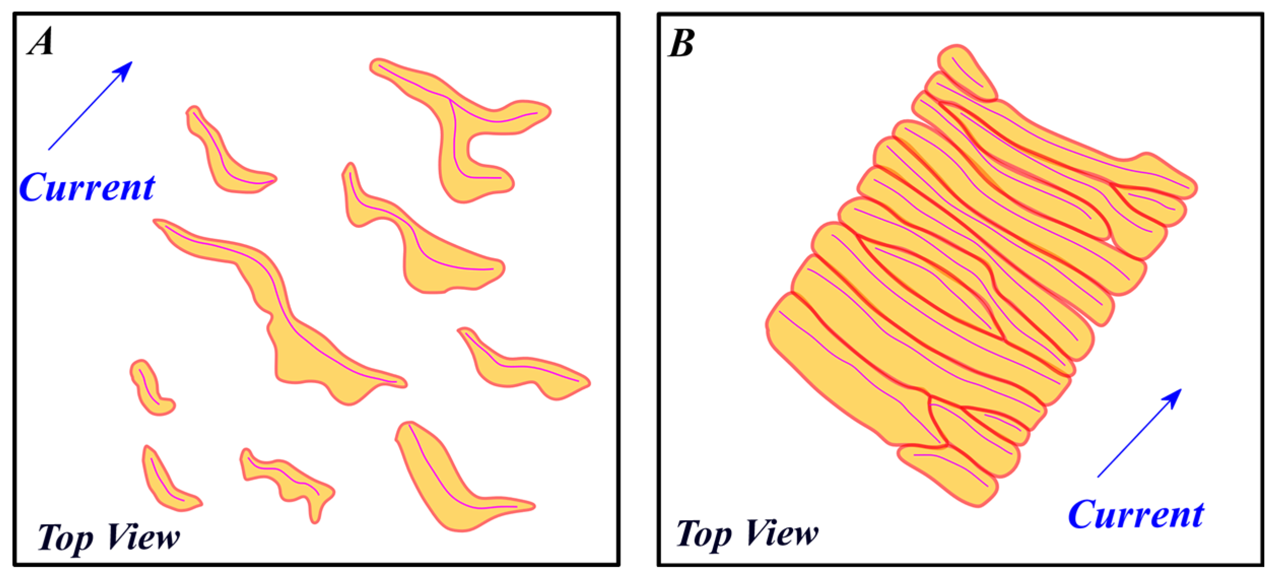
2.2. Morphological Descriptors of the Dunes

Dunes can be characterized once they have been identified and segmented from the DBM. This characterization is based on different morphological descriptors. In this section, we aim to review and describe the morphological descriptors that can be calculated for each dune object as well as the method used for such calculation. Different morphological descriptors of the dunes can be measured considering the salient features used to compute them on the DBM. These morphological descriptors can be estimated in different ways as discussed by [23,25,27]. Indeed, different definitions are applied, depending on the research field and expert knowledge of the analysis. Thus, a formalization of how to estimate these morphological descriptors for the dunes and which features should be considered is required.
Starting with the crest line, its length can be estimated considering its starting and ending points. Furthermore, these points are used to assess the dune orientation angle. This angle can be estimated in two different ways. The first is the dune migration direction relative to the north, as proposed by the authors of [28], illustrated in Figure 4A. The second is the direction of the line passing through the starting and ending point of the crest line of the dune, illustrated in Figure 4B. This second orientation angle is usually perpendicular to the main direction of the current, although angular variations up to 20° can be observed [29,30,31]. The depth corresponds to the distance between the crest line and the water surface. This measure can be estimated based on the depth values of the crest line that can be found on its corresponding pixels in the DBM. In addition, the height of the dunes can be measured as the shortest distance between a crest line and a line joining both troughs [27]. Figure 4 illustrates the descriptors associated with the crest line.
The spacing of the dune on a field and its width can also be computed. The spacing can be estimated as the distance between the crest lines of two consecutive dunes, characterizing the distance between these structures in a field. The width of the dune can be measured as the distance between the stoss and lee trough of the dune [27] or as the horizontal distance between its lee and stoss troughs [1,29,32]. Figure 5 illustrates the spacing and the width of the dunes.
We can also estimate different descriptors for the stoss and lee sides of the dune, as their width and sloping angles [18]. These descriptors are illustrated in Figure 6.
Dunes can also be characterized by different index values, which are calculated based on the dune measurements previously described. The dune symmetry index (1) is defined as the ratio between the stoss and lee side widths [18,26,32].
S y d = W S W L
The symmetry index value usually ranges between 1 and 6. Other definitions of this index may be found in the literature as mentioned by the authors of [29]. The steepness index (2) can be defined as the ratio between the height of the crest line and the width of the dune [29].
S t d = H C W D
The measurements and indices reviewed above are usually defined using a dune profile. Therefore, these sectional views reduce the characterization of the dune to a 2D interpretation, whereas the dunes are 3D structures. Consequently, such measurements and indices vary along the dune structure. Different descriptors exist to describe the morphology of the dunes, such as the already defined length of the crest line. The dune sinuosity index (3) can be estimated based on the ratio between the length of the crest line ( L c ) and the geodetic distance ( D C ) between the crest line extremities [18,29,32].
S i d = L c D C
The measurements considered in the sinuosity index (3) can be observe in Figure 7.

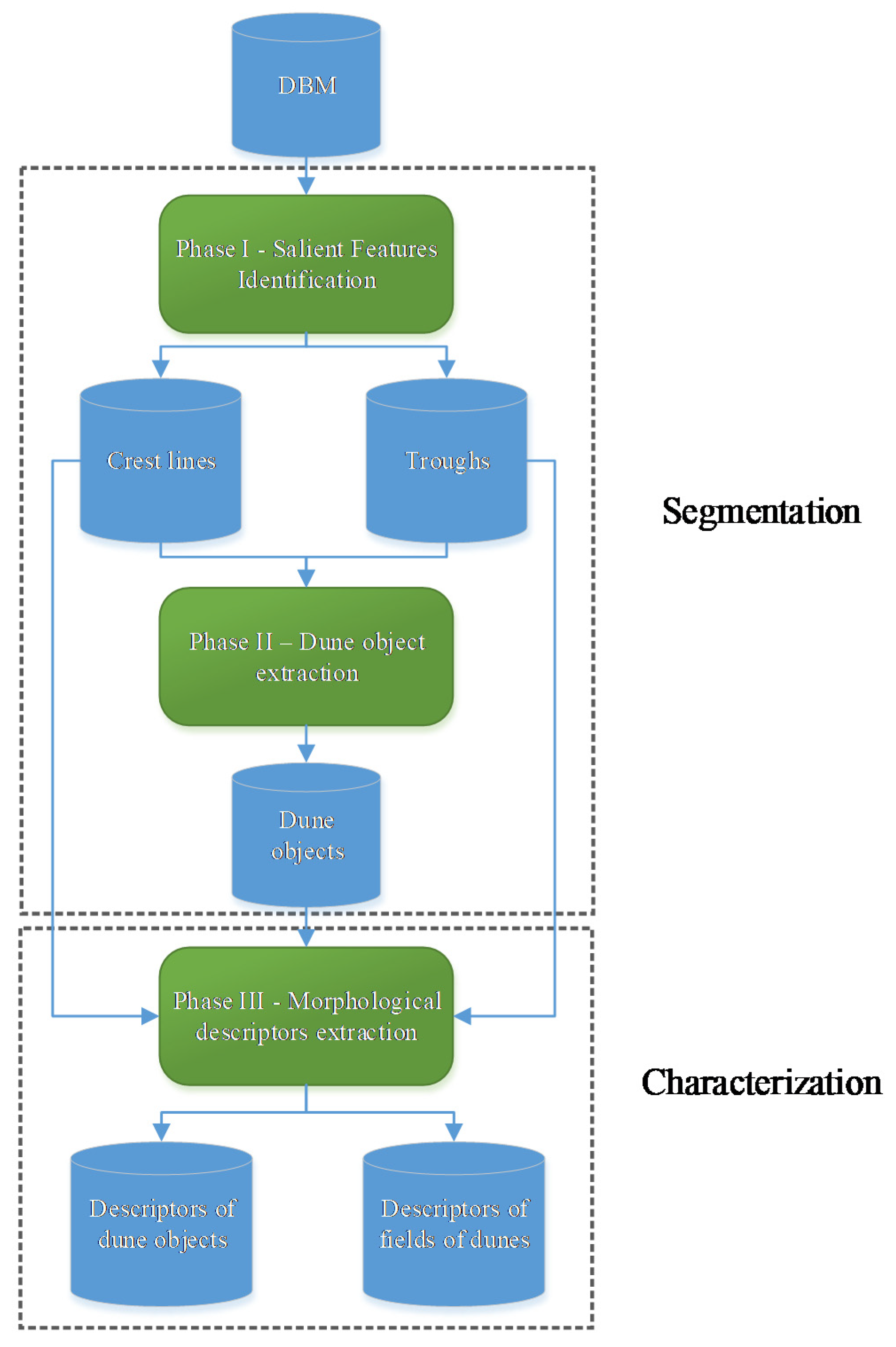
3. Underwater Dunes Characterization from a DBM

This section aims to describe the proposed automatic method to extract the morphological descriptors of the dunes from the seafloor. Our method is divided into two main processes: dune segmentation and dune characterization. This method considers the seafloor surface modelled by a regular gridded DBM. The processes and phases of our method are illustrated in Figure 8.
The first process (i.e., the segmentation approach) considered in the proposed method is described in [17] with the dune landform formalized by a conceptual model. This model considers that a dune can be identified on the seafloor by three salient features, namely, the crest line, stoss trough, and lee trough. The crest line is the linear feature located in the higher zone of the dune. This feature is the upper bound of both sloping sides of the dune (i.e., stoss and lee sides). The stoss and lee troughs represent the boundary of the dune objects, also represented by linear features. These troughs bound the stoss and lee sides, respectively. In the conceptual model, the stoss and lee sides are considered as two components of the dune object. Phase I of the method identifies the three salient features of the dunes from the DBM. In this phase, a morphometric analysis of the seafloor is carried out using the geomorphon algorithm [16]. Salient features are identified after an analysis of the geomorphometric surface and the DBM. Figure 9 illustrates the dune object identified using Phase I processing while considering the dune salient features and components.
Phase II of the method consists of the extraction of the dune object itself considering the salient features identified in Phase I. In this second phase, the troughs are matched with their corresponding crest lines. This matching is carried out by searching the nearest troughs of the crest lines. This search is conducted in the orthogonal direction of the crest line orientation with a predefined range distance limit. Then, the dune object is created by aggregating the pixels located in the area between the crest line and the troughs. In this phase, mathematical morphology and image processing are used to extract the dune object. The result of Phase II is the dune object identified by the same label as its crest line. Figure 10 illustrates an overview of the segmentation approach from the DBM.
Once the dunes have been segmented from the DBM, the second process of the proposed method consists in calculating the morphological descriptors defined in the previous section. Phase III divides these descriptors in two categories. The first one consists of the descriptors of the dune objects, which use the salient features. Here, the following descriptors are used: dune orientation; depth; width; height; stoss and lee angles; stoss and lee widths; asymmetry; sinuosity; and steepness. The second category consists of descriptors that describe how dunes are distributed in the dune field. For that purpose, we propose the following descriptors: the mean spacing between two consecutive dunes; the standard deviation of the dunes spacing; and the dune density of the field.
The following paragraphs explains the extraction, from the DBM, of the main measures used to calculate the morphological descriptors of the dunes. The approach takes advantage of Phase II results, namely the matching of each crest line pixel with its corresponding pixel on the stoss trough and the lee trough, as further illustrated in Figure 11. Please note the use of the median value instead of the mean value for some descriptors, in order to avoid outliers.
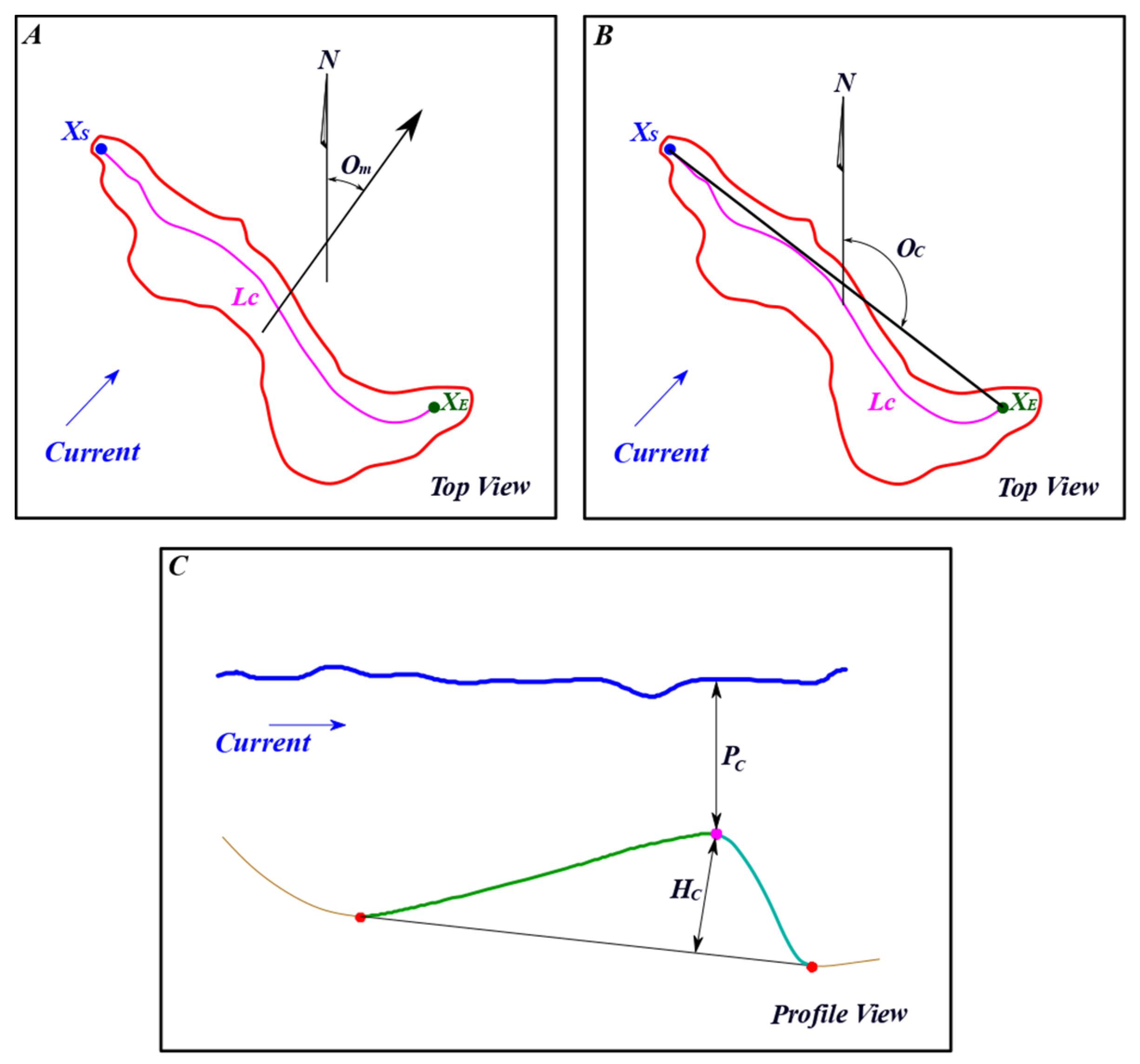
  • The dune orientation is computed using the segment joining the starting and ending pixel of the crest line. We considered the direction facing the lee side of the dune. The segment orientation angle is measured from the north (Om).
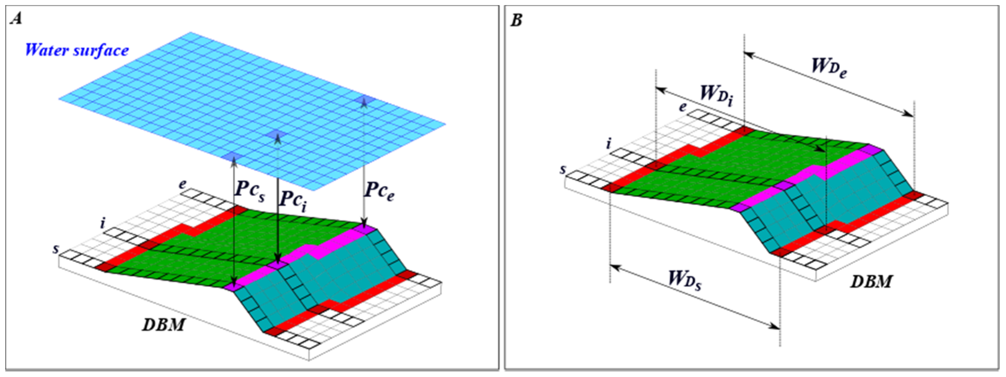
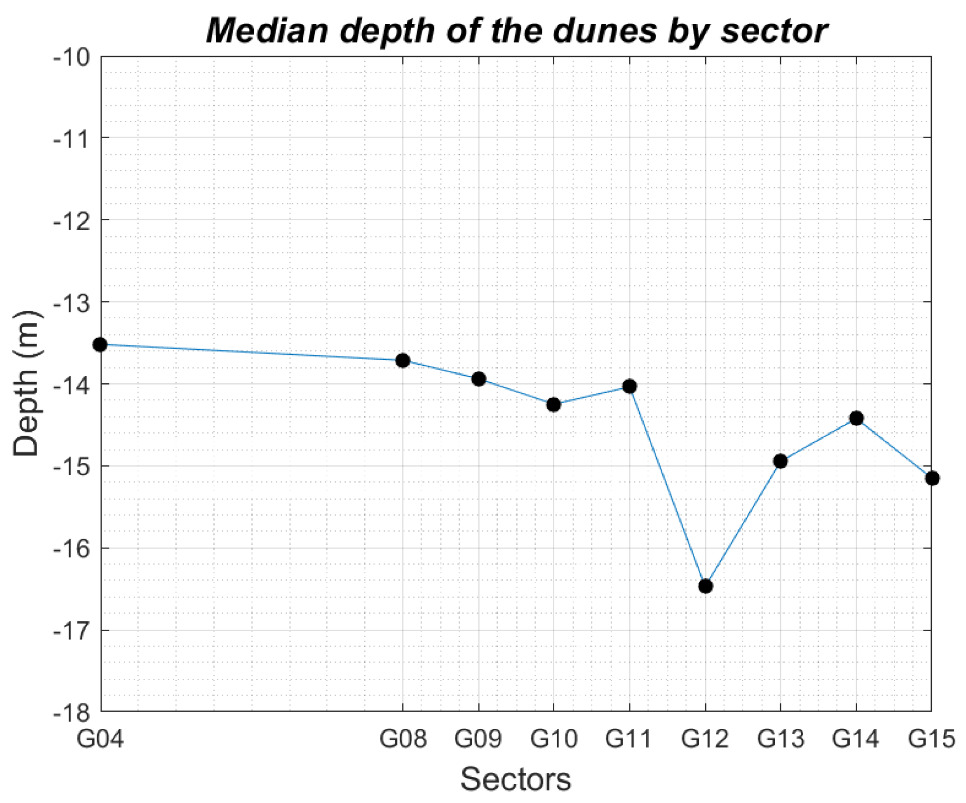
  • The depth (PC) of a dune is computed using the depth of each pixel of the crest line, as illustrated in Figure 11A. The minimum value among these pixels (i.e., closest to the water surface) is considered as the dune depth, since this information is valuable to detect dunes representing a risk for safe navigation.
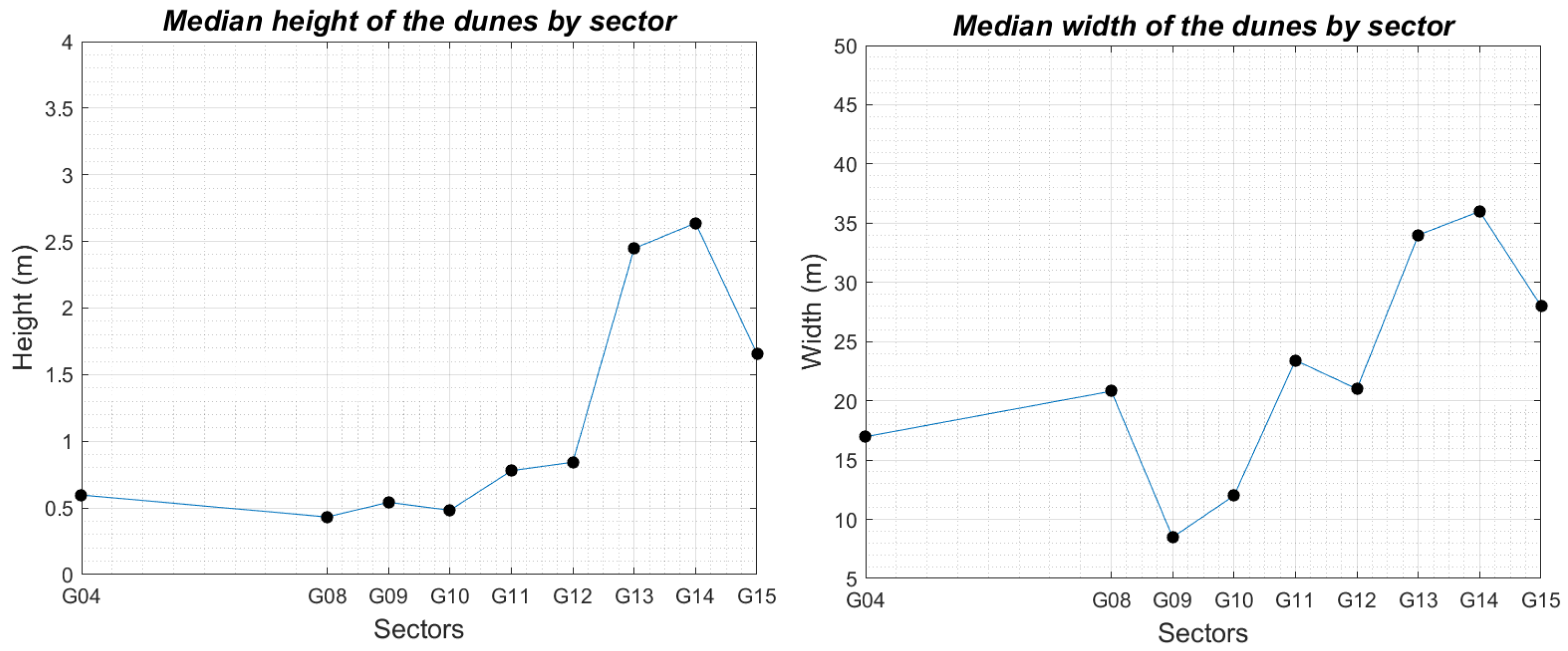
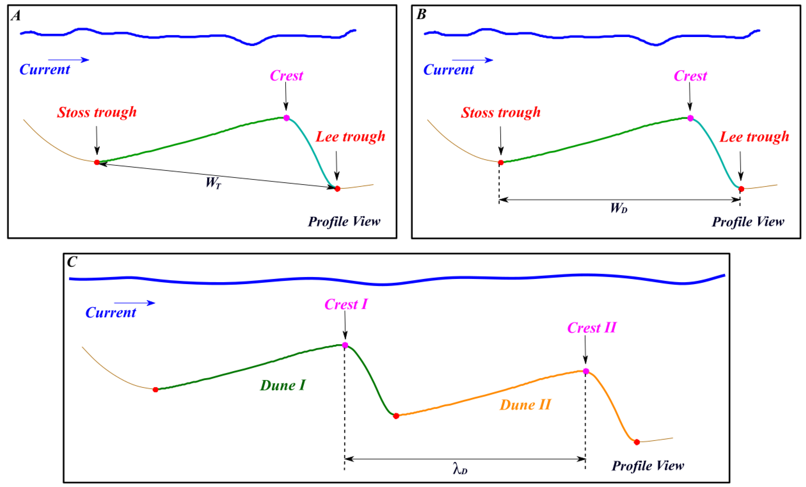
  • The width (WD) is defined as the horizontal distance between the dune lee and stoss troughs. To compute this measure, we considered the stoss and lee trough pixels matched with each crest line pixel. Therefore, a width value is computed for each pixel composing the crest line, as illustrated in Figure 11B. The median value among all crest line pixels is considered as the dune width.
  • The height of a dune (HC) also considers the matching between the pixels of the crest line and the troughs. A height value is computed for each crest line pixel as the distance between the crest line pixel and the line joining the stoss and lee troughs (see Figure 4C). The median value among all the crest line pixels is considered as the height of the dune.
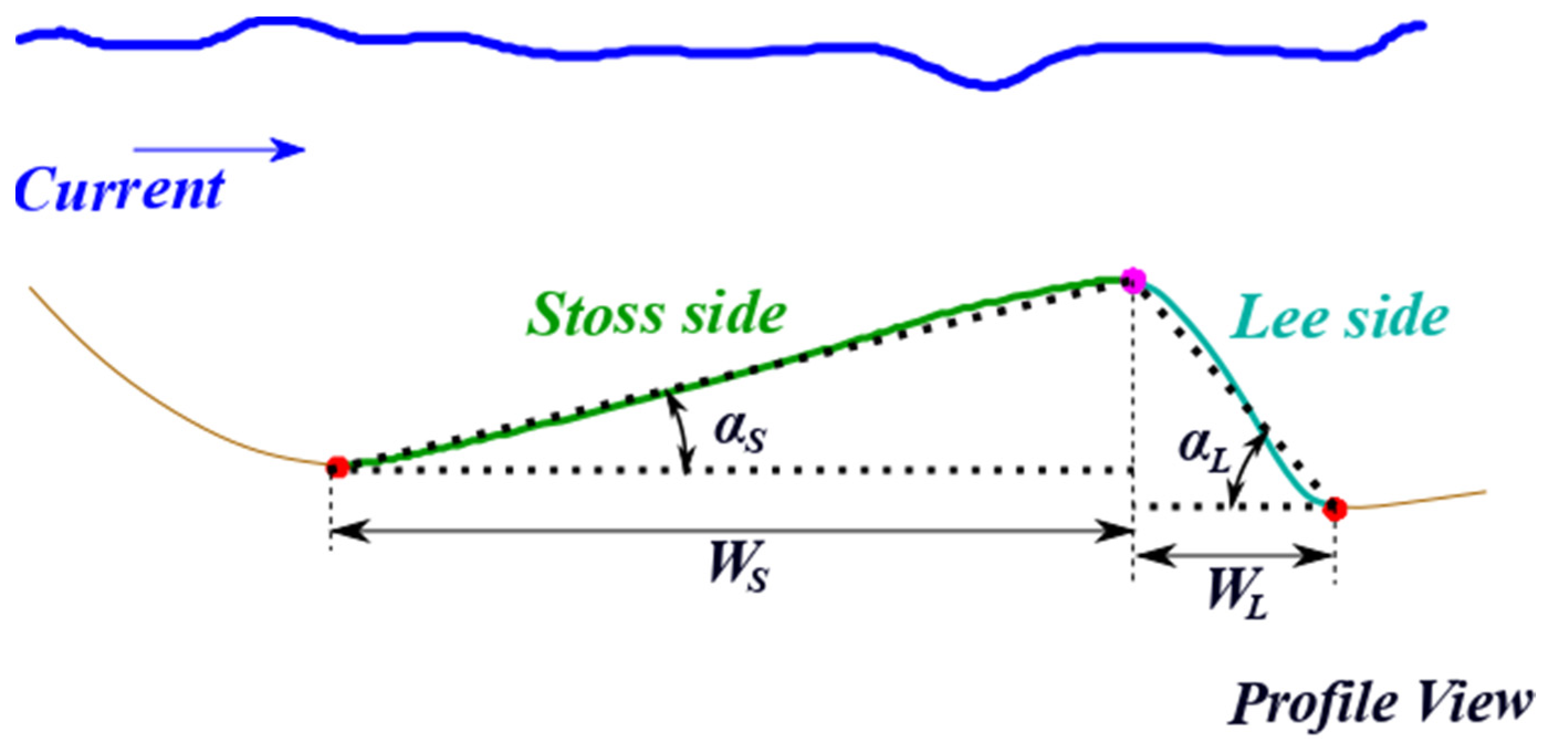
  • The stoss and lee angles (αS and αL), as well as stoss and lee widths (WS and WL), are computed in a similar fashion as the measures related to the crest line. The median values computed are considered as the stoss and lee angles, as well as stoss and lee widths of the dune.
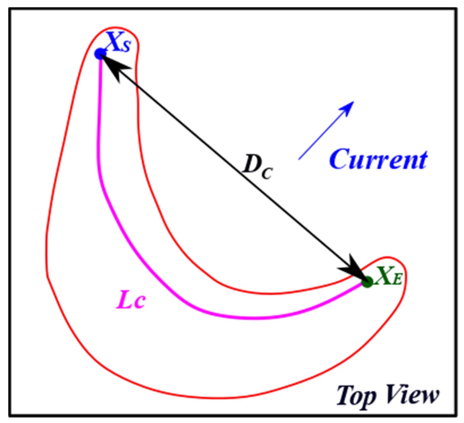
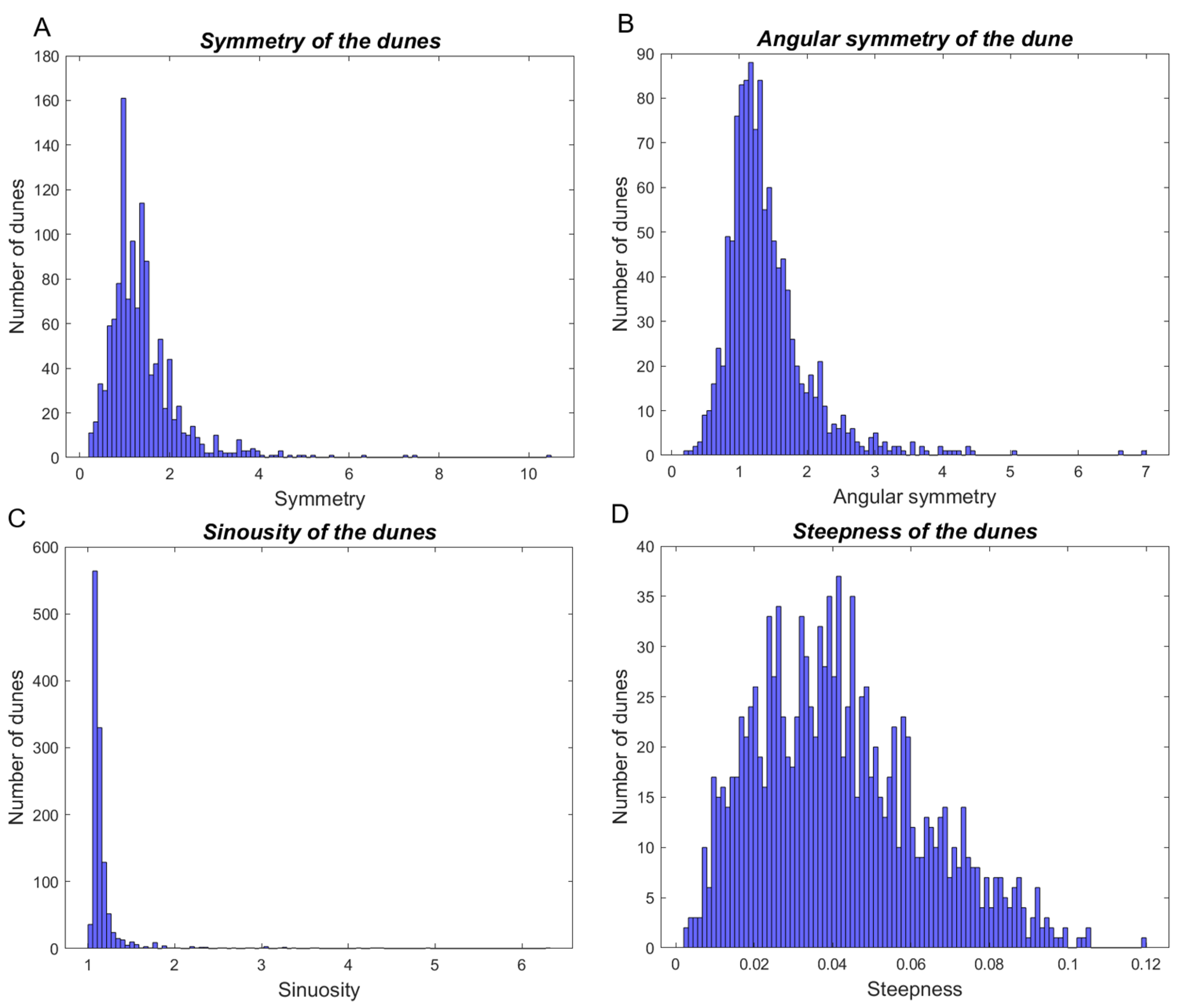
  • The sinuosity index ( S i d ) is computed considering (3). The geodetic distance ( D C ) is calculated as illustrated in Figure 7. Please note that the length of the crest line ( L c ) is not computed as the number of pixels composing the crest line. Instead, the geometric distance between the centers of the pixels is used to increase accuracy given the variability of the crest line sinuosity.
  • The steepness and symmetry indexes are computed for each dune object considering the values previously estimated for the width (WD, WS, and WL) and height (HC), as defined in (1) and (2).
Phase III of the proposed method also extracts the morphological descriptors of the dunes field, as explained in the following paragraphs.
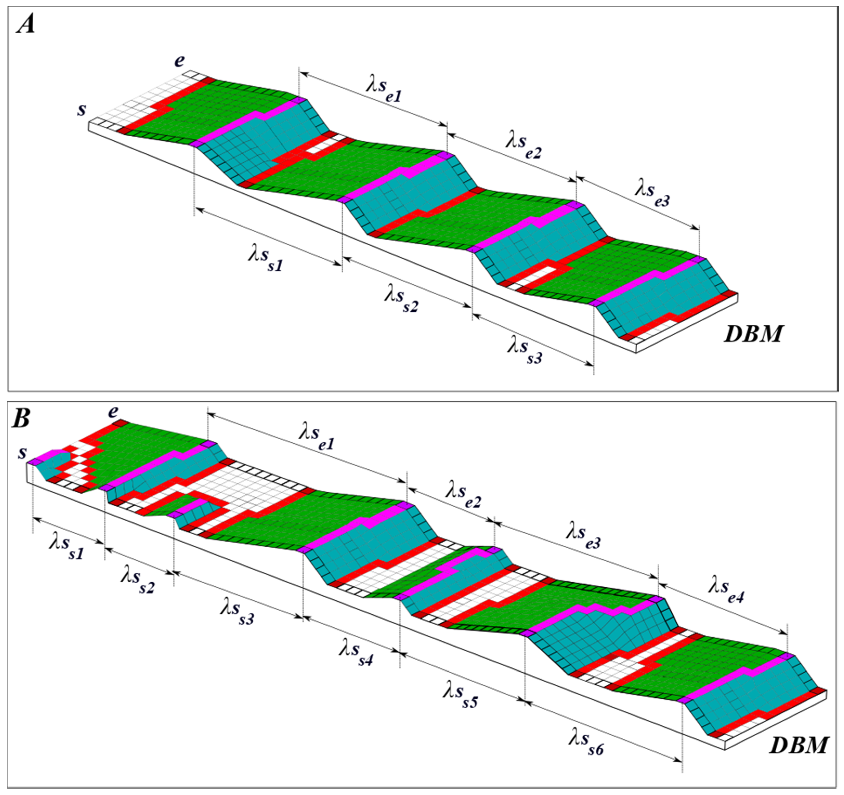
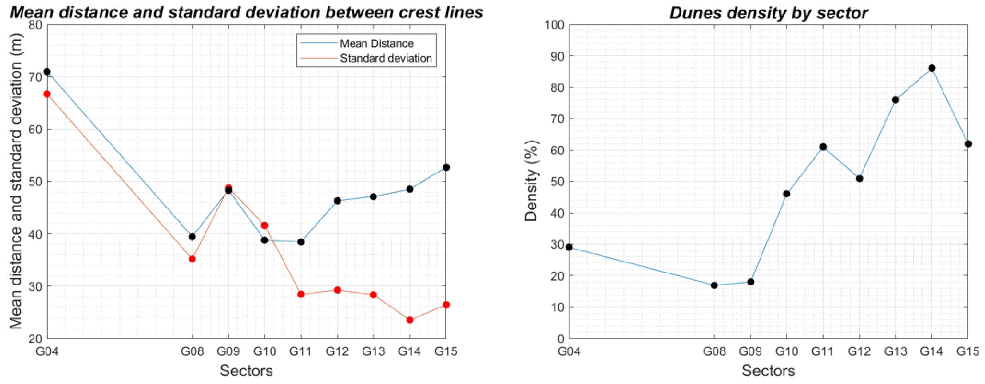
  • The spacing between two consecutive dunes in a field is computed considering the distances between the crest lines of each dune. The computation of the spacing requires a direction. Therefore, the median value of the dune orientation of the objects located on the field is considered here. The spacing is computed for each pixel of the crest lines, as illustrated in Figure 12. Then, the mean value is considered as the spacing (λS) of the dunes of a field.
  • The standard deviation of the spacing ( σ λ s ) is computed considering all the spacing values of the dunes on a field. This descriptor is useful to characterize the dunes dispersion on the seafloor surface.
  • The dunes density ( f D ) is computed using the ratio between the surface of the field covered by dunes ( A C D ) and the total surface of the field ( A f i e l d ), as described in (4). f D is a third-order descriptor mentioned by the authors of [24], therein also called fullbeddedness or fraction of the seafloor covered by dunes.
f D = A C D A f i e l d
In Figure 12, two different dune fields are displayed, i.e., a field where the dunes are adjacent to each other (cf. Figure 12A) and a field with isolated dunes (cf. Figure 12B). Therefore, the spacing between the dunes (λS) is more variable in Figure 12B than in Figure 12A. Consequently, the standard deviation ( σ λ s ) is expected to be higher for isolated dunes (Figure 12B) than adjacent dunes (Figure 12A). In addition, the fraction of the seafloor covered by dunes ( f D ) shall be higher in the field with adjacent dunes (Figure 12A) than in the field with isolated dunes (Figure 12B).

4. Characterization of the Dunes of the Northern Traverse of the Saint Lawrence River

4.1. The Northern Traverse of the Saint Lawrence River

The Saint Lawrence River estuary is a high-dynamic environment, of a length of 400 km, with a width of 15 km at upstream (i.e., north of Orléans Island) and 70 km downstream. The dimensions are such that the hydrodynamic conditions prevailing downstream are typically marine and those upstream are typically estuarine. Different physical agents are responsible for the sediment dynamics in the Saint Lawrence, such as tide, waves, and ice [33]. The zone used to validate the proposed characterization method is the Northern Traverse of the Saint Lawrence River. This navigation channel is located in the transition zone between the river estuary and the middle estuary of the Saint Lawrence River with a width of approximately 305 m and a draft of 12.5 m [34]. This navigation channel was chosen for being a well-surveyed and controlled zone. Therefore, it provides some ground truth to further analyze the morphological descriptors computed with the proposed method in the different sectors of the Northern Traverse. The Canadian Hydrographic Service (CHS) and Ocean Group acquired the data used in this paper in the context of the maintenance of the navigation channel. The surveys mainly aimed to detect and dredge the sedimentary structures that could represent a risk for safe navigation. The available data consists of a regular gridded DBM with a resolution of 1 m.
The Northern Traverse is divided into different sectors. In this paper, nine sectors of the navigation channel are considered with 17 DBMs. Consequently, some sectors have more than one DBM (namely sectors G04, G09, G10, G11, and G14). The DBMs considered in the same sector were acquired at different dates, with a time lapse ranging over a few days to a few years. Even if the DBMs are in the same sector, the sedimentary structures on the surface are different due to the high dynamism of the Saint Lawrence River in the studied zone. In total, 1234 dunes were segmented from the 17 considered surfaces, using the approach proposed by the authors of [17]. This segmentation approach has proven to be efficient with a performance rate of 92% of well-segmented dunes (i.e., true positive). Figure 13 illustrates the location of the different sectors of the Northern Traverse considered in this analysis. It also presents examples of DBMs and segmented dunes for different sectors.
Different configurations of the dunes can be observed in the sectors illustrated in Figure 13. In Sector G04, we can observe more sinuous isolated dunes, with a depth ranging approximately from 13.5 m to 18 m. A few isolated dunes can be observed in sectors G09 and G10, with a depth ranging from approximately 13 m to 16.5 m. In sector G14, adjacent dunes can be observed with a depth ranging from approximately 13 m to 23 m.

4.2. Morphological Descriptors of the Dunes of the Northern Traverse

Once the dunes are segmented (i.e., Phases I and II), the morphological descriptors can be extracted (Phase III), as described in the previous section. In Figure 14, we present the results of the morphological descriptors computation for the 1234 dunes segmented from the 17 DBMs over the nine sectors of the Northern Traverse. Given the large number of dunes, results are displayed as histograms.
The median dune orientation value is approximately 29°, which is in the same direction as the dune migration, as shown in Figure 14A. The depth of the dune objects of the Northern Traverse ranges from 9.95 m to 19.25 m, with a median depth value of 14.02 m, as observed in Figure 14B. The height of the dune objects (Figure 14C) ranges from 3.7 cm to 6.10 m with a median height of 0.74 m, and the width (Figure 14D) varies from 6 m up to 84.85 m with a median width of 21.21 m. The stoss side has a median value of 21 m while the lee side has a median value of 17 m, as observed in Figure 14E. The median value of the stoss angle is 7.68° and the median value of the lee angle is 9.78°, as observed in Figure 14F. Figure 15 presents the histograms with the symmetry, angular symmetry, sinuosity, and steepness indexes of the dune objects.
In addition to the symmetry index (1), the angular symmetry index is calculated using (5).
S y d = α L α L
The reason for calculating both symmetry indexes is related to the segmentation approach. In fact, the segmentation may partially detect the stoss and lee troughs. Consequently, the stoss and lee sides may be partially extracted as well. Such incomplete identification impact significantly the estimation of the width descriptors of the dunes (i.e., WD, WS, and WL). On the contrary, in such context, the angular descriptors each side of the dune can be reliably estimated. The angular symmetry index ranges from 0.20 to 14.2, with a median value of 1.27, as illustrated in Figure 15B. The value of the symmetry index based on the width ranges from 0.2 to 10.5, with a median value of 1.21 (Figure 15A). The reason for having values lower than 1 is due to the imperfect identification of the stoss and lee troughs in the segmentation approach, as previously mentioned. Therefore, in the proposed method, the angular symmetry index is used to characterize the dune objects. The sinuosity index, as illustrated in Figure 15C, ranges from 1.01 to 6.32, with a median value of 1.11. The steepness index ranges from 0.0025 to 0.1197, with a median value of 0.0398 (Figure 15D).
The morphological descriptors previously computed for each dune object may also be used to characterize the fields where they are located. Indeed, by considering each sector of the Northern Traverse as a field, we can group the dunes by sector and consider the median values of their morphological descriptors to characterize each field. Therefore, Table 1 presents the median values of the morphological descriptors of the dune objects according to the field to which they belong.
As previously mentioned, the median migration direction of the 1234 segmented dunes is 29°. Table 1 shows that, while sectors ranging from G08 to G14 have a migration direction fluctuating around 29°, the migration of sectors G04 and G15 is 57° and 201°, respectively. For G04, the migration direction is still consistent with the flow direction of the channel. However, for G15, this direction is in the opposite direction of the preceding sector (G14), which indicates the dominance of the tidal current over the flow direction of the Saint Lawrence River. The dunes located in the southern sectors (i.e., G04 … G10) are generally smaller in height and width, and are also shallower than the dunes of the northern sectors (G11 … G15). This is consistent with the visual analysis of the Northern Traverse nautical charts, as shall be further discussed in the paper. The descriptors directly associated with the fields (i.e., λS, σ λ S , f D ) are also calculated for the nine sectors of the Northern Traverse, as presented in Table 2.
Table 2 shows that the spacing associated with each field of the Northern Traverse ranges from, approximately, 39 m in sector G10 to 71 m in sector G04. The standard deviation of the spacing ranges from approximately 24 m in sector G14 to 67 m in sector G04. In addition, the coverage of dunes on the seafloor ranges from approximately 86% of the seafloor in sector G14 to 17% in sector G08.

5. Analysis and Discussion

This section aims to discuss and analyze the morphological descriptors extracted from the dune objects of the Northern Traverse with the proposed method. The analysis will focus on the fields of the Northern Traverse rather than on the individual dune objects. Indeed, as the results of the previous section have shown, whether it is the morphological descriptors of the dunes or those of the fields, all contribute to characterize the fields to which the dunes belong.
The Northern Traverse being a navigation channel, the depth of the dunes is an important morphological descriptor of these sedimentary structures. Figure 16 presents the median value of this descriptor for each sector of the Northern Traverse. The sectors are ordered sequentially on the x-axis in accordance with their spatial arrangement in the North Traverse (i.e., G04 is the southernmost sector and G15 the northernmost sector). Moreover, consecutive sectors are equally spaced on the x-axis.
As illustrated by Figure 16, the further downstream the sector (i.e., G04 to G15), the deeper the dunes. Therefore, this is consistent, since the navigation channel is located in the transition zone between the river (i.e., shallower) and the estuarine area (i.e., deeper). This finding is also explained by the dynamism of the navigation channel. As specified by experts of this channel, to ensure a minimal depth of 12.5 m, preventive dredging is carried out twice a year. The preventive dredging depth is different for each sector: 13.3 m for sector G04; 13.8 m for sectors G08, G09, and G10; 13.9 m for sectors G11, G12, and G13; and 14.7 m for sectors G14 and G15. In Figure 16, dunes in sector G12 are deeper than dunes located in the neighboring fields. This is consistent with the expert analysis, since the dunes located in this specific sector are naturally deeper without human intervention. Thus, the depth automatically extracted from the 1234 segmented dune objects of the Northern Traverse by the proposed method is consistent with the expert analysis of the sector and with the general description of the Northern Traverse given by [34].
Figure 17 illustrates the median values of the height and width of the dunes for the sectors of the Northern Traverse. The sectors are sequentially ordered and spaced on the x-axis, as displayed in Figure 16.
Figure 17 shows the height and width of the dunes are correlated. Indeed, the highest dunes are in the same sector as the widest dunes, and the narrowest dunes are in the same sector as the smallest dunes. The descriptors of the dunes fields (i.e., λS, σ λ S ,  f D ) are illustrated in Figure 18.
The spacing between dunes (λS) and standard deviation ( σ λ S ) share similar values in the southern sectors (i.e., G04–G10), as illustrated in Figure 18. However, in the northern sectors (i.e., G11–G15), the value of σ λ S is remarkably lower than the value of λS. Thereby, it shows that the dunes on the southern sectors are more spatially dispersed than the dunes on the northern sectors. This conclusion is supported by the fraction of the seafloor covered by dunes ( f D ), as illustrated in Figure 18. The southern fields have less than 50% of their surface covered by dunes. On the contrary, the northern fields have more than 50% of the seafloor covered by dunes. By analyzing these three descriptors (i.e., λS, σ λ S ,  f D ), one can state that the dunes on the northern fields are adjacent to each other, while the southern sectors consist of isolated dunes. This is consistent with the expert knowledge expressed by the professionals responsible for the maintenance of the Northern Traverse. Therefore, this demonstrated that the morphological descriptors, automatically extracted by the proposed method, adequately characterize the dune fields of the navigation channel. Furthermore, such morphological descriptors may be useful to better understand the relationship between the dunes and their hydrodynamic factors. As an example, Figure 19 illustrates the relationship between dunes and the flow current.
Even if Figure 19 is an approximation in terms of current and dune sizes, it is possible to position the sectors of the Northern Traverse based on the dune field descriptor values (cf. Figure 17 and Figure 18). It could be assumed that the flow current increases from sector G08 to sector G15 since dunes in sectors G08 to G12 are smaller than dunes in sectors G13, G14, and G15. The isolated dune objects of the southernmost sector (i.e., G04) may result in a stronger flow current than the sectors located to its north.

6. Conclusions

An automatic characterization method for dunes was proposed in this paper. This method is based on the morphological descriptors of, respectively, the dune objects and the field where they are located. The characterization relies on the dune objects extracted from the DBM by the segmentation approach proposed by the authors of [17]. The proposed method automatically extracts morphological descriptors of the dune objects and the fields where they are located. These morphological descriptors are computed based on the surface of each dune object as well as its three salient features (i.e., crest line, stoss trough, and lee trough). To validate the proposed approach, more than 1200 dunes are characterized over nine fields of the Northern Traverse of the Saint Lawrence River. The dunes and the fields considered in this paper present a significant diversity regarding their characteristics.
The first contribution of our paper is the automatic extraction of the morphological descriptors of the dune objects segmented from a DBM. This automatic extraction with the conceptual model of the dunes prevents the subjectivity of manual calculation. Our method is also more suited to large volumes of data being significantly less time consuming than characterizing dunes visually. The study of dunes located on a field and the characterization of the field itself are useful for the description of the seafloor, as discussed in previous section. The second contribution of the paper is the automatic characterization of the dune fields. Indeed, our method proposes the standard deviation of the spacing ( σ λ S ) as a new descriptor of the fields, complementing those available in the literature (i.e., dune density and spacing of the dunes). In addition, this descriptor can be accurately assessed by taking advantage of the salient features of each dune object. As a result, the characterization of the fields is not only conducted by means of field descriptors, but also by means of individual dune descriptors. As demonstrated, the proposed method provides a reliable and efficient solution to segment and characterize the dune fields and objects from the seafloor surface.
Future work will be dedicated to assessing the performance of the method in contexts other than fluvio-marine, namely marine and fluvial. In addition, its application using DBM at different resolution will also be investigated. Another research direction will concern the use of additional data, such as grain size for different dune fields, backscatter data (as considered by the authors of [36]), current velocity, and tidal information. If these multiple datasets are available with the DBM of the seafloor, it may be possible to improve the characterization method. In correlating the hydrodynamic and environmental factors with dune objects and dune fields, morphological descriptors are used. The correlation between the morphological descriptors discussed in this paper and dune shapes mentioned in the literature (e.g., linear, sinuous, barchan, etc.) may also be investigated further. Finally, the spatiotemporal migration of the underwater dunes may be considered in future research. Indeed, the descriptors computed with the proposed approach may be useful towards the identification of the same dune objects through different surveys.

Author Contributions

Conceptualization: W.N.C.; Methodology: W.N.C.; Validation: W.N.C., S.D., and É.G.; Investigation: W.N.C., S.D. and É.G.; Resources: S.D. and É.G.; Data curation: W.N.C.; Writing—original draft preparation: W.N.C.; Writing—review and editing: W.N.C., S.D. and É.G.; Visualization: W.N.C.; Supervision: S.D. and É.G.; Project administration: S.D.; Funding acquisition: S.D. and É.G. All authors have read and agreed to the published version of the manuscript.

Funding

This research was funded by FRQ-NT (Fonds de Recherche Nature et Technologie Québec), grant number 2018-PR-206875, and the NSERC (Natural Sciences and Engineering Research Council) Discovery, grant number: 2016-05129.

Institutional Review Board Statement

Not applicable.

Informed Consent Statement

Not applicable.

Data Availability Statement

The data are not publicly available. The data were provided courtesy of the Canadian Hydrographic Service and Ocean Group for this research. Code implementation can be provided upon request to the corresponding author.

Acknowledgments

The authors would like to thank Université Laval for providing access to the equipment and laboratories required to conduct this research. In addition, we need to thank, respectively, the Ocean Group and the Canadian Hydrographic Service (CHS), for providing the data used in this research. We must also thank Mitacs, CN (Canadien National), Faculté de Foresterie, Géographie et Géomatique de l’Université Laval, Fond Joncas, l’Association de Géomatique Municipale du Québec (AGMQ), and Canadian Institute of Geomatics (CIG) for their financial support. The authors acknowledge the expert advice in the analysis and discussion phase of the manuscript given by Damien Pham Van Bang from INRS, Sylvain Babineau, and Marie-Ève Biron from Ocean Group and Gabriel Joyal from the Canadian Coastal Gard. Thank you to the companies for the licenses of the software as QPS for Qimera 1.7.6, ESRI for ArcGIS 10.7 and Matlab R2019a—Classroom use.

Conflicts of Interest

The authors declare no conflict of interest.

References

  1. Le Bot, S. Morphodynamique de Dunes Sous-Marines Sous Influence des Marées et des Tempêtes. Processus Hydro-Sédimentaires et Enregistrement. Exemple du Pas-de-Calais. Ph.D. Thesis, Université de Lille I, Villeneuve-d’Ascq, France, 2001. [Google Scholar]
  2. Cheng, H.Q.; Kostaschuk, R.; Shi, Z. Tidal currents, bed sediments, and bedforms at the South Branch and the South Channel of the Changjiang (Yangtze) Estuary, China: Implications for the ripple-dune transition. Estuaries 2004, 27, 861–866. [Google Scholar] [CrossRef]
  3. Boggs, S. Sedimentary structures. In Principles of Sedimentology and Stratigraphy, 4th ed.; Pearson Prentice Hall: Upper Saddle River, NJ, USA, 2006; Chapter 4; pp. 74–116. ISBN 0-13-154728-3. [Google Scholar]
  4. Nichols, G. Processes of transport and sedimentary structures. In Sedimentology and Stratigraphy, 2nd ed.; Wiley-Blackwell, A., Ed.; John Wiley & Sons Publication: West Sussex, UK, 2009; Chapter 4; pp. 44–68. [Google Scholar]
  5. Best, J.L. The fluid dynamics of river dunes: A review and some future research directions. J. Geophys. Res. 2005, 110, F04S02. [Google Scholar] [CrossRef]
  6. Andreotti, B.; Claudin, P.; Devauchelle, O.; Duràn, O.; Fourrière, A. Bedforms in a turbulent stream: Ripples, chevrons and antidunes. J. Fluid Mech. 2012, 690, 94–128. [Google Scholar] [CrossRef] [Green Version]
  7. Lefebvre, A.; Paarlberg, A.J.; Winter, C. Characterising natural bedform morphology and its influence on flow. Geo-Mar. Lett. 2016, 36, 379–393. [Google Scholar] [CrossRef]
  8. Debese, N.; Jacq, J.J.; Garlan, T. Extraction of sandy bedforms features through geodesic morphometry. Geomorphology 2016, 267, 82–97. [Google Scholar] [CrossRef] [Green Version]
  9. Lecours, V.; Dolan, M.F.J.; Micallef, A.; Lucieer, V.L. A review of marine geomorphometry, the quantitative study of the seafloor. Hydrol. Earth Syst. Sci. 2016, 20, 3207–3244. [Google Scholar] [CrossRef] [Green Version]
  10. Debese, N.; Jacq, J.-J.; Degrendele, K.; Roche, M. Toward Reliable Volumetric Monitoring of Sandbanks. In Geomorphometry; Elsevier Science: Boulder, CO, USA, 2018. [Google Scholar]
  11. Yan, G.; Cheng, H.Q.; Jiang, Z.Y.; Tengm, L.Z.; Tang, M.; Shi, T.; Jiang, Y.H.; Yang, G.Q.; Zhou, Q.P. Recognition of fluvial bank erosion along the main stream of the Yangtze River. Engineering 2021, in press. [CrossRef]
  12. Cheng, H.Q.; Chen, W.; Li, J.F.; Jiang, Y.H.; Hu, X.; Zhang, X.L.; Zhou, F.N.; Hu, F.X.; Stive, M.J.F. Morphodynamic changes of the Yangtze Estuary under the impact of the Three Gorge Dam, of estuarine engineering interventions and of climate-induced sea level rise. Earth Planet. Sci. Lett. 2022, 580, 117385. [Google Scholar] [CrossRef]
  13. van Dijk, T.A.G.P.; van Dalfsen, J.A.; Van Lancker, V.; van Overmeeren, R.A.; van Heteren, S.; Doornenbal, P.J. 13—Benthic Habitat Variations over Tidal Ridges, North Sea, the Netherlands. In Seafloor Geomorphology as Benthic Habitat; Elsevier: Amsterdam, The Netherlands, 2012; pp. 241–249. ISBN 9780123851406. [Google Scholar] [CrossRef]
  14. Parsons, D.R.; Best, J.L.; Orfeo, O.; Hardy, R.J.; Kostaschuk, R.; Lane, S.N. Morphology and flow fields of three-dimensional dunes, Rio Paranà, Argentina: Results from simultaneous multibeam echo sounding and acoustic Doppler current profiling. J. Geophys. Res. 2005, 110, F04S03. [Google Scholar] [CrossRef] [Green Version]
  15. Di Stefano, M.; Mayer, L.A. An automatic procedure for the quantitative characterization of submarine bedforms. Geosciences 2018, 8, 28. [Google Scholar] [CrossRef] [Green Version]
  16. Jasiewicz, J.; Stepinski, T.F. Geomorphons—A pattern reconigtion approach to classification and mapping of landforms. Geomorphology 2012, 182, 147–156. [Google Scholar] [CrossRef]
  17. Cassol, W.N.; Daniel, S.; Guilbert, É. A Segmentation Approach to Identify Underwater Dunes from Digital Bathymetric Models. Geoscience 2021, 11, 361. [Google Scholar] [CrossRef]
  18. Lebrec, U.; Riera, R.; Paumard, V.; O’Leary, M.J.; Lang, S.C. Automatic Mapping and Characterisation of Linear Depositional Bedforms: Theory and Application Using Bathymetry from the North West Shelf of Australia. Remote Sens. 2022, 14, 280. [Google Scholar] [CrossRef]
  19. Hains, D.; Bergmann, M.; Cawthra, H.C.; Cove, K.; Echeverry, P.; Maschke, J.; Mihailov, M.E.; Obura, V.; Oei, P.; Pang, P.Y.; et al. Hydrospatial…A global movement. Inter. Hydrogr. Rev. 2021, 26, 147–153. [Google Scholar]
  20. Amos, C.L.; King, E.L. Bedforms of the Canadian eastern seaboard: A comparison with global occurrences. Mar. Geol. 1984, 57, 167–208. [Google Scholar] [CrossRef]
  21. Bartholdy, J.; Flemming, B.W.; Bartholomä, A.; Ernstsen, V.B. Flow and grain size control of depth-independent simple subaqueous dunes. J. Geophys. Res. 2005, 110, F04S16. [Google Scholar] [CrossRef]
  22. Landeghem, K.J.J.; Wheeler, A.J.; Mitchell, N.C.; Sutton, G. Variations in sediment wave dimensions across the tidally dominated Irish Sea, NW Europe. Mar. Geol. 2009, 263, 108–119. [Google Scholar] [CrossRef]
  23. Thibaud, R.; Del Mondo, G.; Garlan, T.; Mascret, A.; Carpentier, C. A Spatio-Temporal Graph Model for Marine Dune Dynamics Analysis and Representation. Trans. GIS 2013, 17, 742–762. [Google Scholar] [CrossRef]
  24. Ashley, G.M. Classification of large-scale subaqueous bedforms: A new look to an old problem. J. Sediment. Petrol. 1990, 60, 160–172. [Google Scholar]
  25. Gutierrez, R.R.; Abad, J.D.; Parsons, D.R.; Best, J.L. Discrimination of bed form scales using robust spline filters and wavelet transforms: Methods and application to synthetic signals and bed forms of the Rio Paraná, Argentina. J. Geophys. Res. Earth Surf. 2013, 118, 1400–1419. [Google Scholar] [CrossRef]
  26. Ferret, Y. Morphodynamique de Dunes Sous-Marines en Contexte de Plate-Forme Mégatidale (Manche Orientale). Approche Multi-Échelles Spatio-Temporelles. Interfaces Continentales, Environnement; Université de Rouen: Rouen, France, 2011. [Google Scholar]
  27. van der Mark, C.F.; Blom, A. A New & Widely Applicable Bedform Tracking Tool; University of Twente, Faculty of Engineering Technology, Department of Water Engineering and Management: Enschede, The Netherlands, 2007; 44p. [Google Scholar]
  28. Knaapen, M.A.F. Sandwave migration predictor based on shape information. J. Geophys. Res. 2005, 110, F04S11. [Google Scholar] [CrossRef] [Green Version]
  29. Ogor, J. Design of Algorithms for the Automatic Characterization of Marine Dune Morphology and Dynamics. Ocean, Atmosphere. Ph.D. Thesis, ENSTA-Bretagne, Brest, France, 2018. [Google Scholar]
  30. Garlan, T. Study on Marine Sandwave Dynamics. Int. Hydrogr. Rev. 2007, 8, 26–37. [Google Scholar]
  31. Garlan, T. GIS and Mapping of Moving Marine Sand Dunes. In Proceedings of the 24th International Cartography Conference, Santiago, Chili, 15–21 November 2009. [Google Scholar]
  32. Berné, S. Architecture et Dynamique des Dunes Tidales. Exemples de la Marge Atlantique Française. Ph.D. Thesis, Université des Sciences et Techniques de Lille Flandres-Artois, Westhoek, France, 1991. [Google Scholar]
  33. Drapeau, G. Dynamique sédimentaire des littoraux de l’estuaire du Saint Laurent. Géographie Phys. Quat. 1992, 46, 233–242. [Google Scholar] [CrossRef] [Green Version]
  34. Comité de concertation navigation de Saint Laurent Vision 2000. Stratégie de Navigation Durable Pour le Saint-Laurent; Ministère des Transports du Québec et Pêches et Océans: Québec, QC, Canada, 2004; 114p. [Google Scholar]
  35. Kenyon, N.H. Sand Ribbons of European tidal Seas. Mar. Geol. 1970, 9, 25–39. [Google Scholar] [CrossRef]
  36. Masetti, G.; Mayer, L.A.; Ward, L.G. A Bathymetry- and Reflectivity-Based Approach for Seafloor Segmentation. Geosciences 2018, 8, 14. [Google Scholar] [CrossRef] [Green Version]
Figure 1. Correlation between the flow velocity, grain size sediment, and the sedimentary structure formed (adapted from [4]).
Geosciences 12 00089 g001
Figure 2. Dune profile with the crest line, the lee and stoss troughs, and lee and stoss sides.
Geosciences 12 00089 g002
Figure 3. Isolated dunes (A) and adjacent dunes (B) on the seafloor. The red lines represent the troughs and the magenta lines represent the crest line of the dunes.
Geosciences 12 00089 g003
Figure 4. Descriptors estimated for the crest line of the dunes. The crest line is displayed in magenta and the troughs in red. XS and XE represents, respectively, the starting and ending points of the crest line. In (A,B), LC represent the length of the crest line. The migration direction of the dune relative to the north (Om) is presented in (A). The orientation angle (OC) of the crest line of the dune, usually perpendicular to the current, is presented in (B). The height (HC) and depth (PC) of the dune are illustrated in (C).
Geosciences 12 00089 g004
Figure 5. Width and spacing of the dunes. In (A), the width is represented by the distance between the dune stoss and lee troughs (WT). In (B), the width is represented by the horizontal distance between the dune lee and stoss troughs (WD). In (C), the width is represented by the spacing measured between two consecutive dunes at their crest lines (λD).
Geosciences 12 00089 g005
Figure 6. Measurements for dune stoss and lee sides. WS, WL, αS, and αL represent, respectively, the width of the stoss side, the width of the lee side, the angle of the stoss side, and the angle of the lee side (adapted from [18]).
Geosciences 12 00089 g006
Figure 7. Measurements considered in the computation of the sinuosity index. L c represents the length of the crest line and X S , X E the starting and ending point of the crest line, respectively. D c represents the geodetic distance between the crest line extremities (adapted from [29]).
Geosciences 12 00089 g007
Figure 8. Proposed method for automatic extraction of dune morphological descriptors and field of dunes morphological descriptors.
Geosciences 12 00089 g008
Figure 9. The dune object identified using its salient features and components. In (A), the dune object on the seafloor is schematized. In (B), the dune object is schematized as identified on the DBM grid. The crest line is in magenta, the trough lines are in red, the stoss sides are displayed in green, and the lee sides are displayed in blue.
Geosciences 12 00089 g009
Figure 10. Data and results for the dune segmentation approach proposed by [17] for the sector G14 of the Northern Traverse. (A,B) illustrate, respectively, the DBM and the salient features of the dunes identified in Phase I; the crest lines are displayed in red and the troughs in blue. In (C), the dune objects segmented in Phase II are presented. Please note that each segmented dune illustrated in (C) are represented with a different color.
Geosciences 12 00089 g010
Figure 11. (A) schematized the extraction of the depth associated with each pixel of the crest line. (B) illustrates the estimation of the width for each cell of the crest line of the dune. The crest lines are in magenta, the trough lines are in red, the stoss sides are displayed in green, and the lee sides are displayed in blue. As previously mentioned, we can observe that for each crest line pixel, our extraction method matched a stoss trough pixel and a lee trough pixel in the morphological descriptors computation.
Geosciences 12 00089 g011
Figure 12. Spacing between the crest lines of two consecutive dune objects. The crest lines are in magenta, the trough lines are in red, the stoss sides are displayed in green, and the lee sides are displayed in blue. λS represents the spacing between dunes while s and e represents, respectively, the starting and ending point of the crest lines. (A) presents adjacent dunes in a field and (B) presents isolated dunes on a field. The dunes in A are more equally spaced than in (B), considering the spacing (λS) between these objects calculated for each pixel of the crest lines.
Geosciences 12 00089 g012
Figure 13. Considered sectors of the Northern Traverse of the Saint Lawrence River as well as 3D representations of some DBMs and segmented dunes (colored objects superimposing the DBM surfaces). To better observe the dunes on the seafloor, a vertical exaggeration of 5 is used in the 3D representations.
Geosciences 12 00089 g013
Figure 14. Histograms of the morphological descriptor values. Please note that in (AD) the descriptors of the dunes are in blue. In (E,F), the stoss descriptors are in blue and the lee descriptors are in red. The additional color (i.e., orange) results from the superposition of the red and blue colors.
Geosciences 12 00089 g014
Figure 15. Histograms of the symmetry indexes. (A): the symmetry index calculated with the width of the stoss and lee sides of the dunes. (B): the angular symmetry index calculated with the angles of the stoss and lee sides. (C): the sinuosity. (D): the steepness values of the dunes.
Geosciences 12 00089 g015
Figure 16. Median-depth of the dunes per sector. Please note that consecutive sectors are equally spaced. Since sectors G05, G06, and G07 are not considered, sectors G04 and G08 are more distant than the other consecutive sectors.
Geosciences 12 00089 g016
Figure 17. Median height and width of the dunes per sector.
Geosciences 12 00089 g017
Figure 18. In the left, the spacing (λS) between the dunes and the standard deviation ( σ λ S ) per sector. In the right, the fraction of the seafloor covered by dunes ( f D ) per sector.
Geosciences 12 00089 g018
Figure 19. Relationship between the dune fields and the flow current (adapted from [1,35]). The fields of the Northern Traverse were placed on the figure based on the size of the dunes.
Geosciences 12 00089 g019
Table 1. Morphological descriptors of the fields of the Northern Traverse sectors. Om is the median orientation, Pc the minimum depth of the crest line, Hc is the median height, WD is the median width of the dunes, S i d is the sinuosity of the dune, and S y a is the angular symmetry of the dunes.
SectorOm (°)PC (m)HC (m)WD (m) S i d S y a
G0457.1813.520.6016.971.161.49
G0833.6913.710.4320.811.111.43
G0921.9213.940.548.491.101.34
G1020.2214.250.4812.001.101.10
G1121.8014.030.7823.421.101.16
G1223.3316.470.8421.001.111.52
G1327.2114.942.4534.001.091.25
G1436.1914.422.6436.001.091.24
G15201.4815.151.6628.001.101.54
Table 2. Spacing between the dune objects (λS), standard deviation ( σ λ S ), and fullbeddedness ( f D ) for the nine dunes fields of the Northern Traverse.
SectorλS (m) σ λ S   ( m ) f D   ( % )
G0470.9566.6629
G0839.4735.1617
G0948.3548.8018
G1038.7841.5846
G1138.4728.4261
G1246.2929.2951
G1347.1328.3576
G1448.5123.5586
G1552.7226.4162
Publisher’s Note: MDPI stays neutral with regard to jurisdictional claims in published maps and institutional affiliations.

