Article

The Influence of Interpolated Point Location and Density on 3D Bathymetric Models Generated by Kriging Methods: An Application on the Giglio Island Seabed (Italy)

by
Emanuele Alcaras
1,*,
Pier Paolo Amoroso
1 and
Claudio Parente
2
1
International PhD Programme “Environment, Resources and Sustainable Development”, Department of Science and Technology, Parthenope University of Naples, Centro Direzionale, Isola C4, 80143 Naples, Italy
2
DIST—Department of Science and Technology, Parthenope University of Naples, Centro Direzionale, Isola C4, 80143 Naples, Italy
*
Author to whom correspondence should be addressed.
Geosciences 2022, 12(2), 62; https://doi.org/10.3390/geosciences12020062
Submission received: 28 December 2021 / Revised: 23 January 2022 / Accepted: 27 January 2022 / Published: 29 January 2022

Abstract

:
In relation to 3D bathymetric modelling, this article aims to analyze the performance of Kriging approaches in dependence of the location and density of the measured depth points. The experiments were carried out on a multi-beam sonar (MBS) dataset that includes 240,000 soundings covering a sea-bottom area near Giglio Island (Italy). Seven subsets were derived in random way from the initial regular MBS dataset, selecting an increasing number of points uniformly spaced. Seven models were generated for both Ordinary Kriging and Universal Kriging. Each model was submitted to leave-one-out cross-validation to define the exactness of the predictive values and compared with the initial grid to better evaluate the accuracy in dependence of the point number and dissemination. To investigate this relationship, a new index called MVI (Morphological Variation Index) was introduced as a measurement of the level of variation of seabed morphology. The results validate the efficiency of the Kriging methods and remark the influence of the dataset distribution on the 3D model, highlighting MVI as a useful index to represent the seabed variation as a unique value. Finally, in no rugged areas using 1 point every 1000 m2, the RMSE of the differences between measured and interpolated values falls below 1 m, while a further increment of soundings is required in the presence of a high level of variation of seabed morphology.

1. Introduction

Nowadays, 3D modeling is applied in many fields, such as cultural heritage preservation [1], underground survey [2], coastal monitoring [3], indoor mapping [4], quarry’s studies [5], and landfill monitoring [6].
Three-dimensional models include digital elevation models (DEMs) that are typically used to visualize the variation of the Earth’s surface [7] and produced through many procedures such as remote sensing, photogrammetry, and land surveying [8]. A continuous representation of the examined part of the Earth surface is typically generated using appropriate interpolators that can be applied to topographic data as well as to hydrographic data [9].
Interpolation is founded on the principles of spatial autocorrelation, which assumes that closer points are more similar compared to farther ones [10], in accordance with the first law of geography formulated by Tobler [11]. In other terms, we can define spatial interpolation as the procedure to predict the value of attributes at unobserved points within a study area covered by existing observations [12]. Using points with known values (sample points), interpolation techniques allow for predicting unknown values for any geographic point data, such as elevation, rainfall, chemical concentrations, noise levels, etc. [13]. Typically applied to grids with estimates made for all cells, interpolation methods generate a surface from the points [14]. They have been classified as global or local [15]. The difference between the two groups lies in the use of points with known values for assessing unknown values: a global method uses all the data available in the initial dataset while a local method uses only a selection of them, typically the points closest to the single grid node in which the value must be calculated [16]. Interpolation methods are also classified as either exact or approximate methods because of the characteristic of preserving or not preserving the original sample point values on the inferred surface [17]. Another distinction is made between deterministic and stochastic methods. The former use point values directly and can be applied when there is sufficient knowledge about the geographical surface being modeled so as to describe its character as a mathematical function [18]. The latter utilize the statistical properties of the measured points: they quantify the spatial autocorrelation among sample points and consider the spatial configuration of the measured points around the prediction location [19].
Some of the most used deterministic methods are: Inverse Distance Weighting (IDW), local polynomial functions (first, second, third, …, nth order), and radial basis functions [20]. Particularly, IDW estimates interpolated points considering their distance from known values: each measured point is weighted by the inverse of its distance from the interpolation point [21]. Consequently, as the distance increases, the weight decreases rapidly [22].
Polynomial interpolation fits a smooth surface defined by a mathematical function (a polynomial) to the input sample points [23]. The order of the polynomial ranges from first-order to higher-order: in every case, the values of the coefficients included in the polynomial equation must be determined using the measured values in the sample points [24]. Global polynomial functions use the entire dataset to define the equation of a single surface capable of representing the entire area by itself. Local polynomial functions use a local subset defined by a window rather than all the measured points: the window is moved across the analyzed region, positioned on each grid node, and the surface value at the center of this moving box is assessed. The window is so large that it contains a sufficient number of data points for defining the surface equation [25], e.g., no less than 10 points for a third-order polynomial function [26].
Radial basis functions are conceptually similar to fitting a rubber membrane through the measured sample points while minimizing the total curvature of the surface [27]. They include different basis functions (e.g., completely regularized spline, spline with tension thin-plate spline, multiquadric function, inverse multiquadric function, etc.) and depending on which you select, it will determine how the rubber membrane will fit between the values [15]. Radial basis functions are exact interpolators, thus they require the surface to pass through the measured points; however, they can predict values above the maximum and below the minimum measured values.
Geostatistical methods include the concept of randomness, whereby the interpolated surface is hypothesized as one of many that might have been observed and all of which could generate the known data points [28]. Some of the most used stochastic methods are Ordinary Kriging and Universal Kriging [29]. Particularly, since they were used for the experiments carried out in our research, these methods are described in detail in the next section.
Several interpolation algorithms are available in literature and a large part of them is already implemented in GIS software, but the choice of the most suitable of them cannot be made a priori since it requires them to be evaluated each time [26]. Their use concerns terrain as well as sea-bottom representation.
Three-dimensional bathymetric models, which are investigated in this article, are fundamental for many purposes: the spatial representation of the seabed morphology allows for the development of studies such as those on navigation safety [30], coastal dynamics [31], sea ecosystems [32], seagrass meadows mapping [33], port dredging [34], infrastructure projects [35], etc.
Depth data that can be interpolated for 3D bathymetric model creation are usually acquired by the hydrographic authority through bathymetric survey and used for nautical chart production. The acquisition of bathymetric data of the sea surrounding the Italian peninsula and the construction of the relative nautical charts is the prerogative of the “Istituto Idrografico della Marina Militare” (I.I.M.M.), which is the hydrographic authority in Italy [36].
Bathymetric surveys can be carried out using different types of instrumentation based on acoustic signal transmission through the water; single-beam sonar (SBS) [37], multi-beam sonar (MBS) [38], and side-scan sonar (SSS) [39] are widely diffused techniques for hydrographic survey that supply datasets for seabed representation. Furthermore, bathymetric data can be extracted from multispectral satellite images (Satellite Derived Bathymetry, SDB) [40] or from the Electronic Navigational Chart (ENC) [41]. SBS, MBS, and SSS convert into a range the measurement of the time lag between transmitting and receiving an acoustic signal that travels through the water, springs back the seabed, and returns to the sounder [42,43]. SDB is carried out by processing the remotely sensed images using specific techniques, such as the band ratio method [44], which takes into account the relationships between bands [45].
Single-beam data as well as depth data derived from a nautical chart are point cloud datasets that are submitted to spatial interpolation processes that allow for generating 3D models [46]. Those irregularly spaced measured points are used as input to calculate the depths in the nodes of appropriate grids that are spaced in relation to the accuracy of the input data [26,47]. In other terms, established by the extension of the study area, the accuracy of the generated model is proportional to the number of nodes that compose the grid covering this area: the greater the number of nodes, the better will be the output model. Obviously, particular attention must be paid to choosing this number because it is of no use to create a 1000 × 1000 grid if the map only contains three sounding values [48].
The accuracy of the resulting 3D models is affected by the points numerosity and distribution [49]. In literature, mathematical models are proposed to take into account several independent variables, such as the surface slope, the density of points, the spatial distribution of these points, and the interpolation method, in order to explain the accuracy of a given DEM [50]. Aguilar et al. (2002) [51] recognized three factors that influence the accuracy of a DEM: the morphology of the terrain, the density of the measured points, and the interpolation method used. Several studies have been conducted on the influence of points density for DEMs generation and a large part of them considers laser scanner techniques, particularly LiDAR (Light Detection and Ranging) applications [52,53,54]. Regardless of the acquisition technique used to capture measured points, some studies focus on the relationship between the DEM accuracy and the sampling density. Aguilar et al. (2005) analyzed this relationship and analytically adjusted it to a decreasing potential function [55]. Chaplot et al. (2005) evaluated the performance of interpolation techniques for the generation of the DEM of natural landscapes of differing morphologies and over a large range of scales [56]: five interpolation techniques (inverse-distance weighting, Ordinary Kriging, Universal Kriging, the multiquadratic radial basis function, and regularized spline with tension) were applied and their performance evaluated using data for both a mountainous area of northern Laos and a gentle landscape of western France at nested spatial scales, with sampling densities from 4 to 109 points/km2.
This article aims to analyze the performance of Kriging approaches for bathymetric data interpolation in dependence of the location and density of the sample points related to the morphological situations. Each algorithm available in GIS software to interpolate height/depth values has its own advantages and disadvantages [57] but Kriging interpolators are included among the most performing ones [58], thus we preferred to use two of them in this study, namely Universal Kriging and Ordinary Kriging. Experiments were carried out on MBS datasets covering a sea-bottom area near Giglio Island (Italy) and results analyzed in reference to the sounding density. A new index named the Morphological Variation Index (MVI) is proposed to numerically express the level of variation of the seabed morphology to establish the useful number of points to be interpolated in dependence of the bottom conformation.

2. Study Area and Datasets

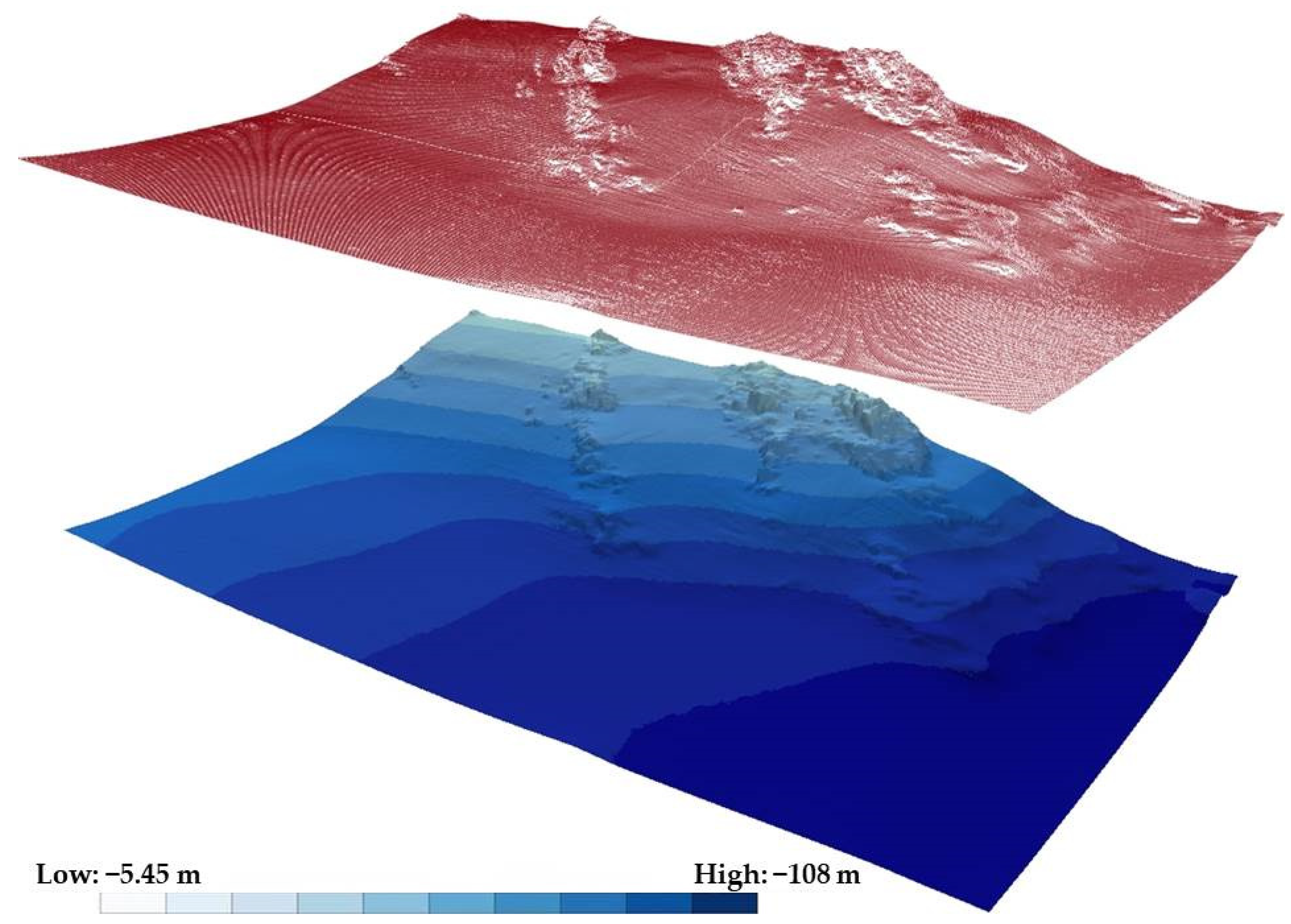
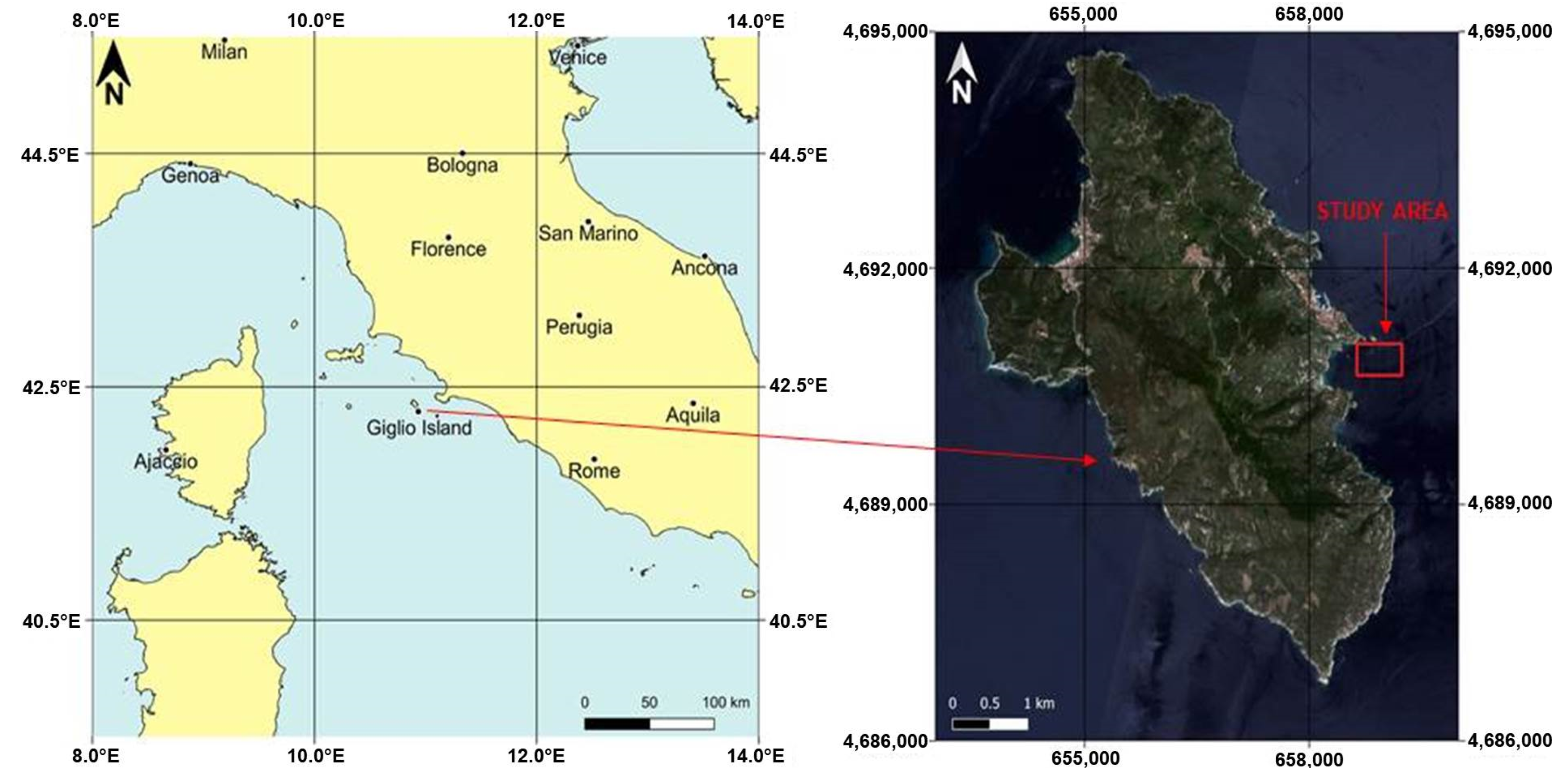
The experiments are carried out on a MBD that includes 240,000 measured points (Figure 1) and covers an area of the sea bottom near the coasts of the Giglio Island (Italy) in the Tuscan archipelago (Figure 2), with an extension of 240,000 m2 (one point per square meter). The original dataset counts a total of 825,602 points and is provided by I.I.M.M., who also carried out the bathymetric survey in 2012.
The study area was chosen because it is of great interest; in fact, several hydrographic campaigns have been carried out on it over time. Furthermore, this area is characterized by a high level of variability of the seabed; in fact, it has both particularly steep and jagged areas, and some almost flat areas [59]. The sea bottom, beneath 50 m of depth, consists of more than 60% clay [60].
The area extends 400 m × 600 m within the following UTM/WGS84 plane coordinates −32T zone: E1 = 658,640 m, E2 = 659,240 m, N1 = 4,690,639 m, and N2 = 4,691,039 m.
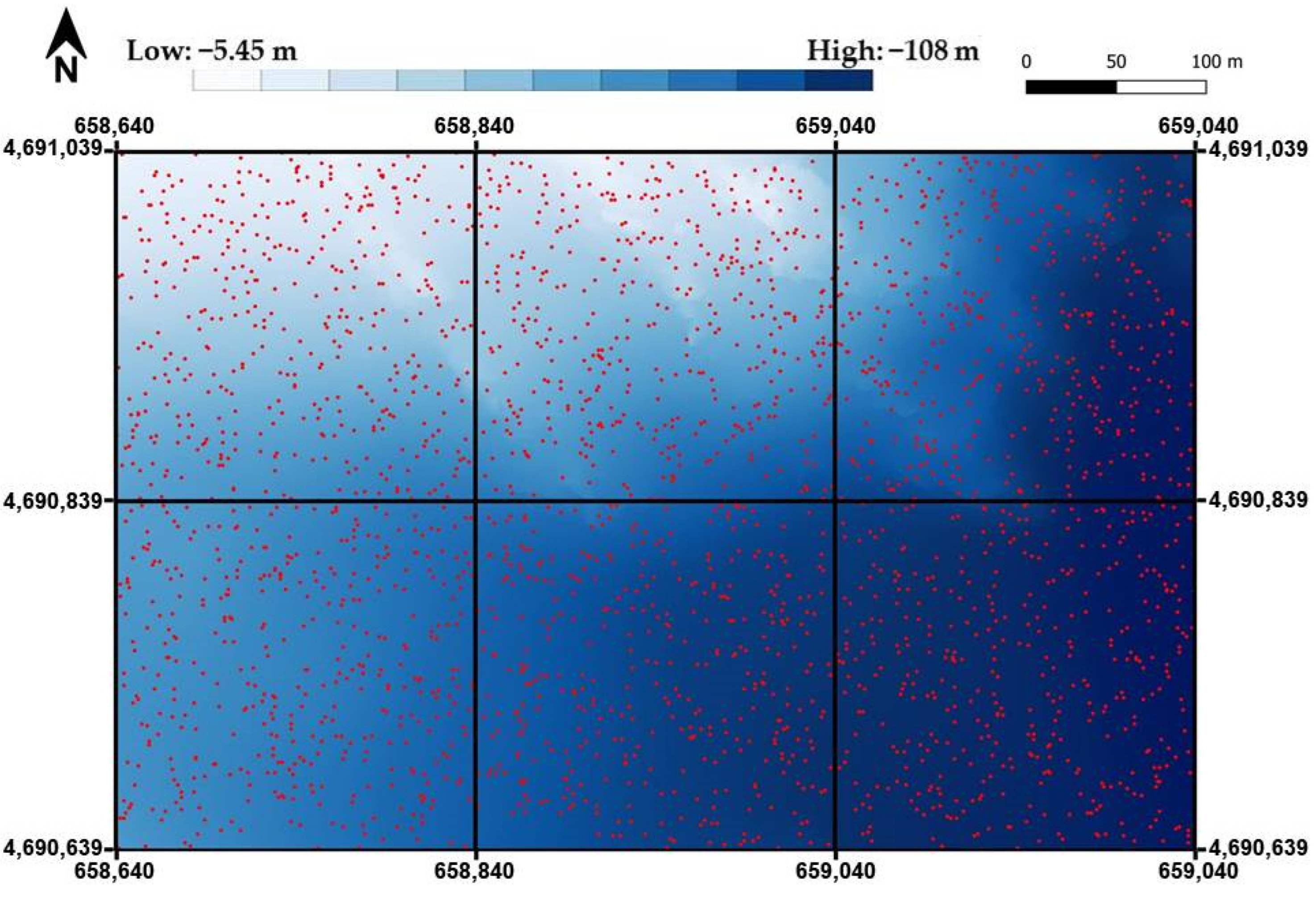
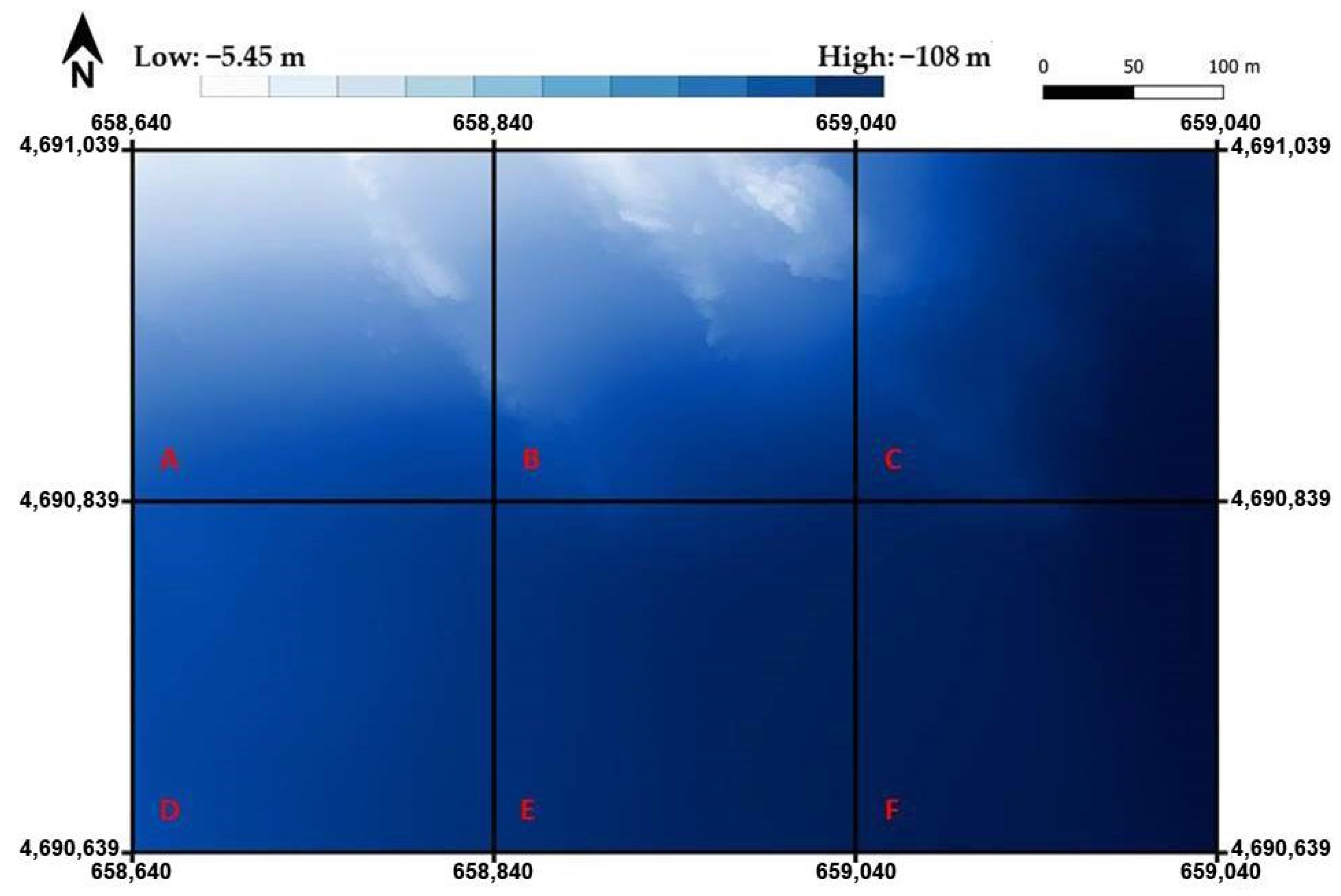
MBS data were organized as grid points containing X, Y, and Z values. Depth values range between −5.45 m and −108 m in the selected area, with a precision of 1 cm on depths. Different subsets were derived in random way from the initial MBS, selecting an increasing number of points (24, 48, 120, 240, 480, 1200, and 2400). Particularly, the area was subdivided in six sectors extending 200 m × 200 m (Figure 3) and the selection was carried out to ensure an equal number of points included in each sector. As shown in Section 3 and Section 4, this data organization permits us to identify different morphological situations so that each sector can represent a local typical variability of the seabed.

3. Methods

Each of the seven subsets described above was submitted to Kriging interpolation to obtain 3D bathymetric models of the study area. Using the extension of ArcGIS [61], named Geostatistical Analyst [62], seven models were generated for both Ordinary and Universal Kriging. Each model was submitted to leave-one-out cross-validation [63] to define the exactness of predictive values; in addition, each product was compared with the initial grid to better evaluate the accuracy of the model in dependence of the point number and dissemination. The experiments were carried out to investigate the efficiency of the Kriging methods and analyze the impact of both the dataset location and density on the 3D model exactness. Particularly, we explored the influence of the variability of the seabed morphology on the measured point number and distribution in order to achieve accurate results.
In the following sections, the proposed approach to produce 3D bathymetric models and to investigate their accuracy in dependence of sample point location and dissemination is described in detail. First of all, main characteristics of Kriging interpolation (Section 3.1) are resumed; then, the steps for model construction and global accuracy evaluation are illustrated (Section 3.2.1); and finally, the proposed index for analyzing the morphological variation of the seabed (MVI) based on the inversions of the slope and the extent of the differences in depth between adjacent pixels is illustrated, remarking its rule for evaluating the local accuracy of the 3D bathymetric model produced (Section 3.2.2).

3.1. Kriging Interpolation

The Kriging interpolation method is based on the application of a geostatistical model which takes into account the spatial correlation between the sampled points and adapts it to estimate the value at an unsampled point [64].
The fundamental principle of Kriging is to assume that the spatial variation of any attribute is too irregular to be modeled by a simple mathematical function [65]. This irregular variation can be modelled, often achieving better results, by applying a stochastic surface [29]. Indeed, Kriging is one of the stochastic interpolation methods and for this reason, it is based on the principle according to which the link between neighboring points can be expressed by a statistical correlation which does not necessarily express physical meaning [66]. For Kriging, this turns out to be a very efficient technique and one of the most used in many fields of application, such as: data reconstruction [67], rainfall intensity estimation [68], temperature spatial modelling [69], soil composition variability [70], and DEM generation [71].
In order to evaluate the variability of the attributes of the points as the distance increases, Kriging makes use of the semi-variogram [72]. The semi-variogram is a diagram in which the semi-variance is represented as a function of the distance between two points [73]. The semi-variance function is given by the following formula [74]:
γ ( h ) = 1 2 n i = 1 n ( z ( x i ) z ( x i + h ) ) 2
where γ(h) is the value of the semi-variance at the distance d; n is the number of couples of points separated by d; z is the value of the depth; and xi and xi + h indicate the positions of each couple of points.
There are several different Kriging techniques and all are developed as variations of simple Kriging [75]. Among these, we decided to apply Ordinary Kriging and Universal Kriging approaches.

3.1.1. Ordinary Kriging

Ordinary Kriging is one of the most commonly used Kriging techniques. It is defined as the best linear unbiased estimator (BLUE): best because it aims at minimizing the variance of the errors, linear because its estimates are weighted linear combinations of the available data, and unbiased since it tries to have the mean residual or error equal to zero [76].
Ordinary Kriging serves to estimate a value at a point of a region for which a variogram is known using data in the neighborhood of the estimation location [77]. In other words, its aim is to predict the value of the random variable z ( x 0 ) at an unsampled point x 0 of a geographical region [78].
The function z ( x i ) is composed of a deterministic component µ and a random function ɛ ( x i ) [79]
z ( x i ) = μ + ε ( x i )
The deterministic component is a constant value for each x i location in each region of study.
Ordinary Kriging is based on two assumptions:
(1)
The global, constant mean μ     R of the random function Z(x) is unknown; and
(2)
The data derive from an intrinsically stationary random function Z(x) with known variogram function γ(h).
Thus, the equation that defines the model assumed by Ordinary Kriging is:
z ( x 0 ) = i = 1 n w i z ( x i )
where w i provides the unknown weights corresponding with the influence of the variable z ( x i ) in the computation of z ( x 0 ) .
The value of each output pixel is calculated through different steps [80].
Firstly, the algorithm determines the input points for each pixel output, calculates the distances between all of them, and find the semi-variogram value for those distances. The semi-variogram values are filed out in the following matrix:
( 0 γ ( h 12 ) γ ( h 13 ) γ ( h 21 ) 0 γ ( h 23 ) γ ( h 31 ) γ ( h 32 ) 0 γ ( h 14 ) γ ( h 1 n ) γ ( h 24 ) γ ( h 2 n ) γ ( h 34 ) γ ( h 3 n ) γ ( h 41 ) γ ( h 42 ) γ ( h 43 ) γ ( h n 1 ) γ ( h n 2 ) γ ( h n 3 ) 0 γ ( h 4 n ) γ ( h n 4 ) 0 )
where
  • n is the number of the input point;
  • i = 1, 2, …. n;
  • j = 1, 2, … n;
  • h i j ( h 11 ,   h 12 ,   h 13 ,   ,   h 21 ,   h 22 ,   h 23 ,   ) is the distance between input point i and input point k; and
  • γ ( h i j )   ( ( γ ( h 11 ) ,   ( γ ( h 12 ) ,   ( γ ( h 13 ) ,   ,   ( γ ( h 21 ) ,   ( γ ( h 22 ) ,   ( γ ( h 23 ) , ) is the value of the semi-variogram for the distance between input point i and input point k.
The distances of the output pixel towards all input points are calculated and the semi-variance for these distances extracted from the semi-variogram are filled out in vector D:
( γ ( h p 1 ) γ ( h p 2 ) γ ( h p 3 ) γ ( h p 4 ) γ ( h p n ) )
where
  • h p i ( h p 1 ,   h p 2 ,   h p 3 ,   ,   h p n ) is the distance between the output pixel p and input point i and
  • γ ( h p n )   ( ( γ ( h p 1 ) ,   ( γ ( h p 2 ) ,   ( γ ( h p 3 ) ,   ,   ( γ ( h p n ) ) is the value of the semi-variogram for distance h p i between the output pixel p and input point i.
The following matrix equation is solved to calculate the weight factors:
( 0 γ ( h 12 ) γ ( h 13 ) γ ( h 14 ) γ ( h 1 n ) 1 γ ( h 21 ) 0 γ ( h 23 ) γ ( h 24 ) γ ( h 2 n ) 1 γ ( h 31 ) γ ( h 32 ) 0 γ ( h 34 ) γ ( h 3 n ) 1 γ ( h 41 ) γ ( h 42 ) γ ( h 43 ) 0 γ ( h 4 n ) 1 1 γ ( h n 1 ) γ ( h n 2 ) γ ( h n 3 ) γ ( h n 4 ) 0 1 1 1 1 1 1 1 0 ) · ( w 1 w 2 w 3 w 4 w n λ ) = ( γ ( h p 1 ) γ ( h p 2 ) γ ( h p 3 ) γ ( h p 4 ) γ ( h p n ) 1 )
where w i is a weight factor for input point i and
λ is a Lagrange multiplier introduced to minimize possible estimation error.
This matrix equation can be written as a set of n + 1 simultaneous equations:
i ( w i · γ ( h i j ) )
i w i = 1
Then, the algorithm calculates the estimated or predicted value Z of the output pixel as the sum of the products of the weight factors and the input point values using the Equation (2).

3.1.2. Universal Kriging

While Ordinary Kriging assumes that the mean µ is constant across the entire region of study, this method assumes that the mean μ ( x ) has a functional dependence on the spatial location and can be approximated by a model with the equation [81]:
μ ( x ) = l = 1 k a l f l ( x )
where
  • a l is the coefficient to be estimated from the data (generally unknown) and characterizes the local trend (drift coefficient);
  • f l is the lth basic function (generally polynomials) of spatial coordinates that describes the drift; and
  • k is the number of functions used in modelling the drift.
For this method, Equation (2) can be rewritten as follow [82]:
z ( x i ) = μ ( x i ) + ε ( x i )
The local trend or drift can be expressed by a polynomial; in the case of a quadratic expression, Equation (9) can be rewritten as:
μ ( x ) = a 0 + a 1 x i + a 2 y i + a 3 x i 2 + a 4 x i y i + a 5 y i 2
where
  • x i   , y i   are the x, y coordinates of the input points and
  • a 0 ,   a 1 ,   ,   a 5 are the unknown drift coefficients.
In the case of linear expression, Equation (11) can be rewritten as:
μ ( x ) = a 0 + a 1 x i + a 2 y i
As for the Ordinary Kriging and also in this case, the weights must be calculated. Considering 5 input points and a local linear trend, the set of equations in matrix form is:
0 γ h 12 γ h 13 γ h 14 γ h 15 1 x 1 y 1 γ h 21 0 γ h 23 γ h 24 γ h 25 1 x 2 y 2 γ h 31 γ h 32 0 γ h 34 γ h 35 1 x 3 y 3 γ h 41 γ h 42 γ h 43 0 γ h 45 1 x 4 y 4 γ h 51 γ h 52 γ h 53 γ h 54 0 1 x 5 y 5 1 1 1 1 1 0 0 0 x 1 x 2 x 3 x 4 x 5 0 0 0 y 1 y 2 y 3 y 4 y 5 0 0 0 · ( w 1 w 2 w 3 w 4 w 5 λ a 1 a 2 ) = ( γ ( h p 1 ) γ ( h p 2 ) γ ( h p 3 ) γ ( h p 4 ) γ ( h p 5 ) 1 x p y p )
where
  • n is the number of the input point;
  • i = 1, 2, … n;
  • j = 1, 2, … n;
  • h i j ( h 11 ,   h 12 ,   h 13 ,   ,   h 21 ,   h 22 ,   h 23 ,   ) is the distance between input point i and input point k;
  • ( h p 1 ,   h p 2 ,   h p 3 ,   ,   h p n ) is the distance between the output pixel p and input point i, and is the value of the semi-variogram for the distance between input point i and input point k;
  • γ ( h p n )   ( ( γ ( h p 1 ) ,   ( γ ( h p 2 ) ,   ( γ ( h p 3 ) ,   ,   ( γ ( h p n ) ) is the value of the semi-variogram for distance hpi between the output pixel p and input point i;
  • x i   , y i   are the x, y coordinates of the input points;
  • a 0 ,   a 1 ,   ,   a 5 are the unknown drift coefficients; and
  • x p   , y p   are the x, y coordinates of the output pixel.
This matrix form must be solved for each output point in the same way as described for Ordinary Kriging. The weights are crucial to calculate an estimated or predicted value in each pixel of the output map using Equation (2).

3.2. Adopted Methodological Approach

3.2.1. Model Construction and Global Accuracy Evaluation

For this work, 7 models were generated using Ordinary Kriging and 7 models using Universal Kriging, namely one for each selected subset of points. All operations were carried out in the GIS environment: Geostatistical Analyst, the extension of ArcGIS that adds advanced tools for exploratory spatial data analysis and the interpolation process aimed at creating a statistically valid surface [83], allowed us to generate optimal models from sample data and evaluate predictions for better decision making. Geostatistical Analyst permitted us to apply Ordinary Kriging as well as Universal Kriging; in addition, it allowed us to choose the most performing semi-variogram model that results in both interpolators’ stable model. The grid cell was fixed at 1 m taking into account the characteristics of the initial dataset. However, in addition to the morphology of the seabed, the number of points necessary for the 3D modeling must take into account the resolution of the final model [55]; consequently, if the number of points per km2 is limited, it is necessary to fix a very large cell size. Nevertheless, in our study, the attention was focused on the influence of the morphology of the seabed on the determination of the number of points needed, therefore the grid cell was set at 1 m in every case and the number of points used for modeling varied from time to time. The choice of the pixel dimension equal to 1 m allows for the direct comparison of the constructed models with the starting grid obtained from the multibeam survey.
To assess the accuracy of the results, two approaches were carried out:
-
Cross validation (CV); and
-
Direct comparison with the MBD.
In the first case, cross-validation permits the defining of the accuracy level of predictive values [84]. In other words, it is a statistical validation technique used to assess how well an interpolation model performs [85]. Different methods are available in literature for CV application [86,87,88,89,90]. Particularly, the leave-one-out (LOO) method is adopted, removing each point in turn from the dataset and using the other points to estimate a value at the location of the removed point [91].
In the second case, the original model obtained with all the points of the initial dataset (MBD) was compared with the seven models obtained both for the Ordinary Kriging and Universal Kriging depending on the number of points taken into consideration. In other words, the difference between the original one and each of the seven obtained models was performed using a raster calculator, which is the powerful ArcGIS tool that allows you to create and execute an expression of the map algebra [92] that will output a raster.
The performance of both approaches is evaluated using statistical terms such as mean, standard deviation, minimum, maximum, and Root Mean Square Error (RMSE). RMSE is considered the most widely used global accuracy measure for evaluating the performance of DEMs and is calculated in accordance with the formula [55,93,94]:
R M S E = i = 1 N ( Z i ( x , y ) Z i ( x , y ) ) 2 N
where
  • N is the number of the depth points (that, in this case, coincides with the number of the grid cells);
  • Zi (x,y) is the measured depth at the location i(x, y); and
  • Z i ( x , y ) is the interpolated depth at the same location i(x, y).

3.2.2. Morphological Variability and Local Accuracy Evaluation

The impact of the density of the points on the modeling of the seabed differs according to the variation of the seabed: the higher the variation, the higher is the number of points necessary for modelling.
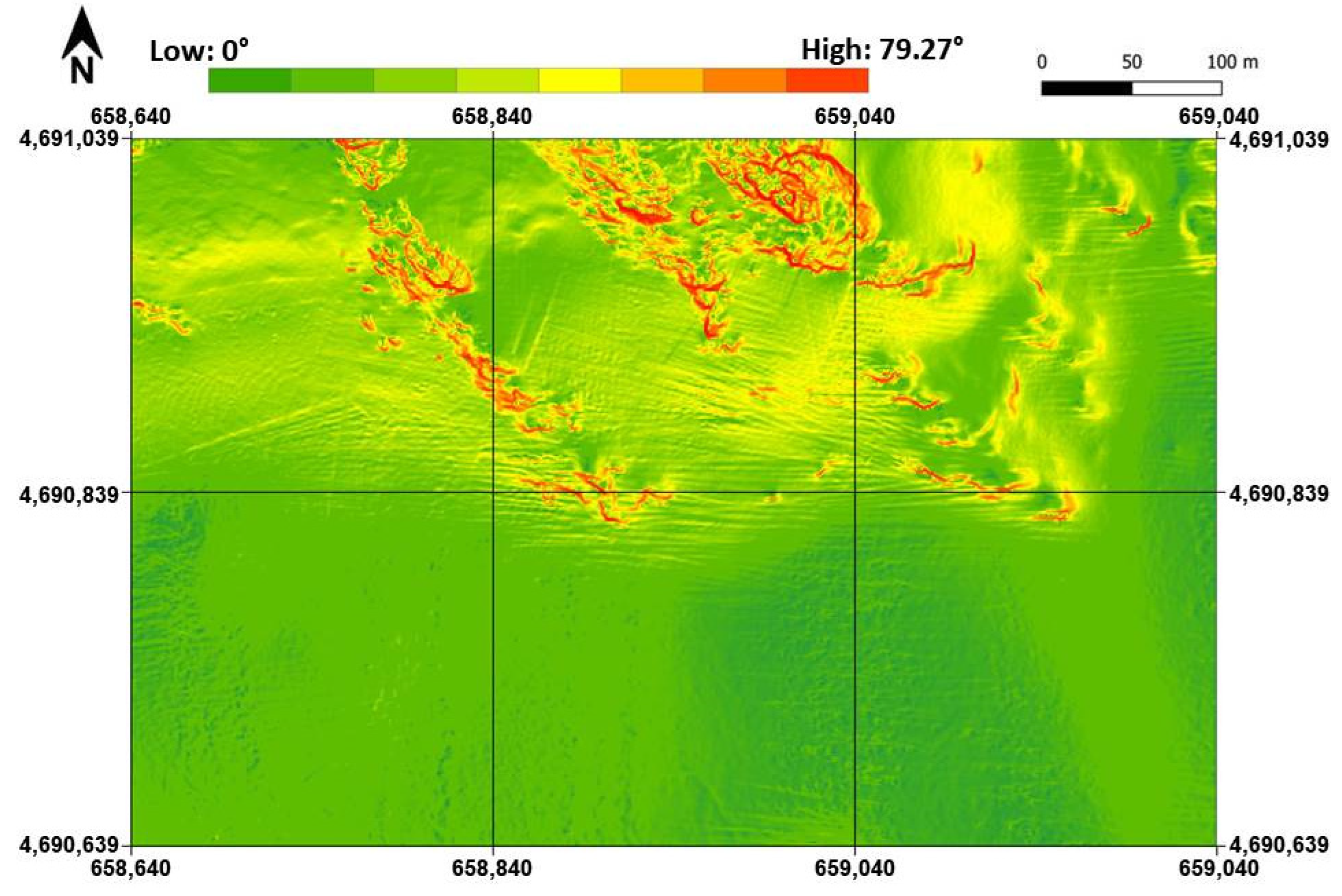
The study area chosen for this work presents seabed with variegated slopes, as shown in Figure 4.
The proposed organization of the initial data into 6 subsets, each covering an area (sector) of 200 m × 200 m, is representative of the seafloor configuration since each of them remarks local trends and characterization of the morphology. The identification of these sectors with the letters A, B, C, D, E, and F is shown in Figure 5.
Each sector has different seafloor patterns; for example, sector B has large variations in depth while sector D has less abrupt and more linear variations in depth.
Subsequently, the analysis of the residuals between the initial dataset and the individual models was conducted in relation to each of the six sectors into which the area has been divided so as to highlight the variability of the results also in relation to the specificity of the morphology of the seabed.
In literature, different morphometric variables are described for DEM analysis and their use is also possible for Digital Depth Model (DDM) analysis. Lozano Parra et al. (2009) [95] considered three parameters to classify landforms: slope gradient (Digital Slope Model, DSM), curvature (Digital Curvature Model, DCM), and roughness (Digital Roughness Model, DRM). DSM represents the slope angle and is usually calculated as the maximum rate of change between the altitude of each cell and its neighbors, expressed in degrees; basically, the maximum change in elevation over the distance between the cell and its eight neighbors identifies the steepest downhill descent from the cell [96]. The DCM represents the concavity or convexity of a surface and can be calculated using a fourth-degree polynomial function fitted to the surface [97]. The DRM not only expresses the range of elevation in the vertical direction (z) but also reflects its variation and irregularity [98]; it can be defined as the variation rate of the slope in a specific area and no standard method exists to calculate it [95]. The terrain roughness index (TRI) proposed in [99] calculates the quantitative measurement of terrain heterogeneity for every location by summarizing the change in elevation within the 3 × 3 pixel grid: each pixel contains the difference in elevation from a center cell and the eight cells surrounding it.
In order to analytically express the heterogeneity of the analyzed surface, a new index is introduced in this work, named the Morphological Variation Index (MVI). This index takes into account two components: the first component (Ixy) is related to the variation of the direction of the slope (ascending or descending) while the second component (Sxy) takes into account the variation of the value of the slope. Both these components are considered in relation to x and y directions.
MVI is given by the following formula:
M V I = I x y · S x y
Regarding the component Ixy, the difference between the consecutive pixel values is considered along the x direction (i.e., along each row) and along the y direction (i.e., along each column); if this difference always has the same sign, the direction does not change, i.e., the seabed continues to rise or fall. By assigning the value 0 to the conservation of the direction and 1 to its variation, the sum of all the values divided by the total number of the pixels of the grid gives a percentage value that expresses the variability of the seabed in terms of the frequency of the ascend–descent inversion. Since two values are calculated (one for the x direction and the other for the y direction) for each pixel, Ixy is the mean of them, referring to all the grid cells.
Regarding the component Sxy, the difference between the consecutive pixel values (depth values) related to the pixel dimension is considered along the x direction as well as the y direction to calculate slope. Then, the variation of slope is determined and normalized by dividing each value by the maximum (theoretical) value, which is 180°. Additionally, in this case, two values were calculated (one for the x direction and the other for the y direction) for each pixel, thus Sxy is the mean of them, referring to all the grid cells.
Finally, once the interpolator is fixed (Ordinary Kriging or Universal Kriging), six values of Ixy, six values of Sxy, and, consequently, six values of MVI are calculated, namely one for each sector.

4. Results and Discussion

The statistic values of all the residuals for each dataset are shown in Table 1 for Ordinary Kriging applications analyzed by cross-validation and in Table 2 for the same applications analyzed by direct comparison. Similarly, statistic values of all the residuals for each dataset are shown in Table 3 for Universal Kriging applications analyzed by cross-validation and in Table 4 for the same applications analyzed by direct comparison.
By examining the RMSE values, the results confirm the efficiency of both considered Kriging methods, remarking the augmentation of the accuracy level related to the increment of the number of measured points in the same area. Ordinary Kriging applications produce RMSE values that rapidly decrease from the first to the seventh subset (from 4.489 m to 0.503 m using cross-validation and from 4.053 m to 0.537 m using direct comparison). Universal Kriging models present similar trends of the residuals related to the measured point density, even if the results are slightly less accurate as testified by the RMSE values (from 5.105 m to 0.628 m using cross-validation and from 4.863 m to 0.647 m using direct comparison).
By analyzing the other statistics of the residuals, it is evident that the direct comparison produces very high maximum and minimum values. This effect is due to the particular morphology of the considered area that is extremely rugged in one of the six sectors (B), with a rapid alternation of ups and downs as well as abrupt changes in slopes.
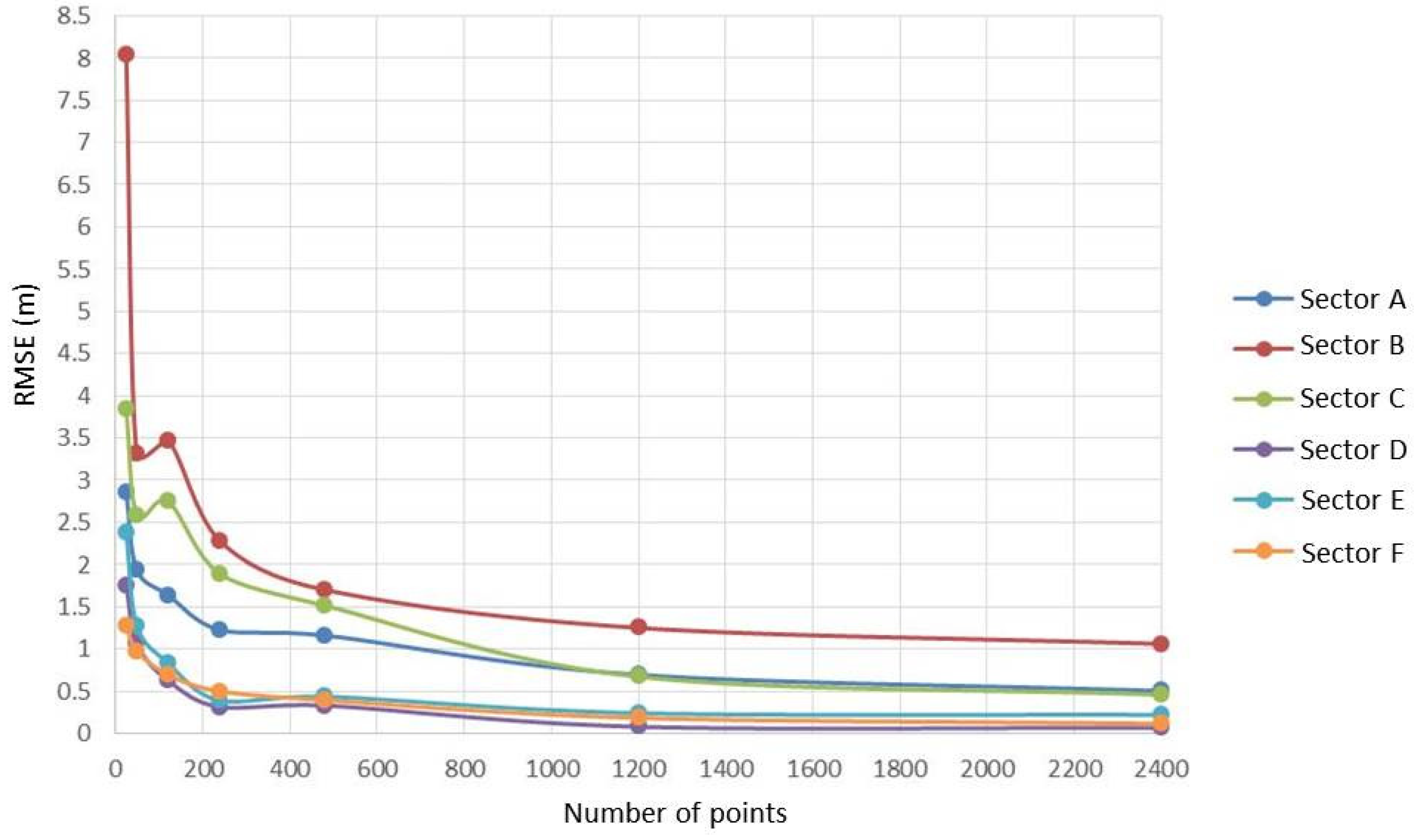
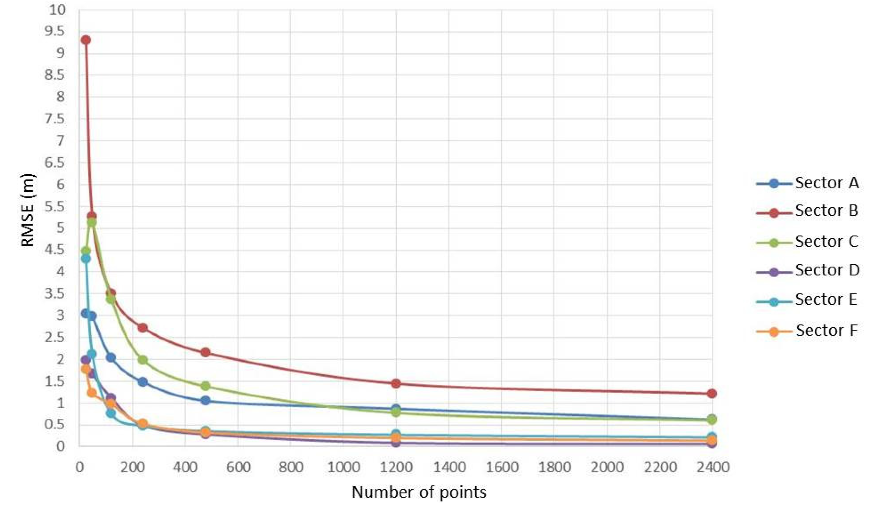
For this reason, a statistical analysis was carried out for each sector through direct comparison with MBD. In particular, Figure 6 and Figure 7 show the trend of the RMSE as a function of the number of points obtained in each sector for Ordinary Kriging and Universal Kriging, respectively.
In both cases, the data clearly show that the highest values of RMSE are obtained in sector B while the lowest in sector D: for this reason, we report in Table 5 and Table 6 the statistical values relating to these two sectors with 2400 points used.
In analyzing the RMSE values as the number of points varies, it is noted that as the points increase, the RMSE generally decreases, except for some special cases, due to the particular conformation of the seabed and by the totally random distribution of the points. Ordinary Kriging provides slightly better results than Universal Kriging in all sectors. Regardless of the adopted method, it is possible to notice how the RMSE values drop below 1 m when already using 1200 points, except in sector B. By doubling the number of points, the RMSE values in the second sector still remain above 1 m, even if, in the case of the Ordinary Kriging, the RMSE is only 61 mm above the meter (1.061 m).
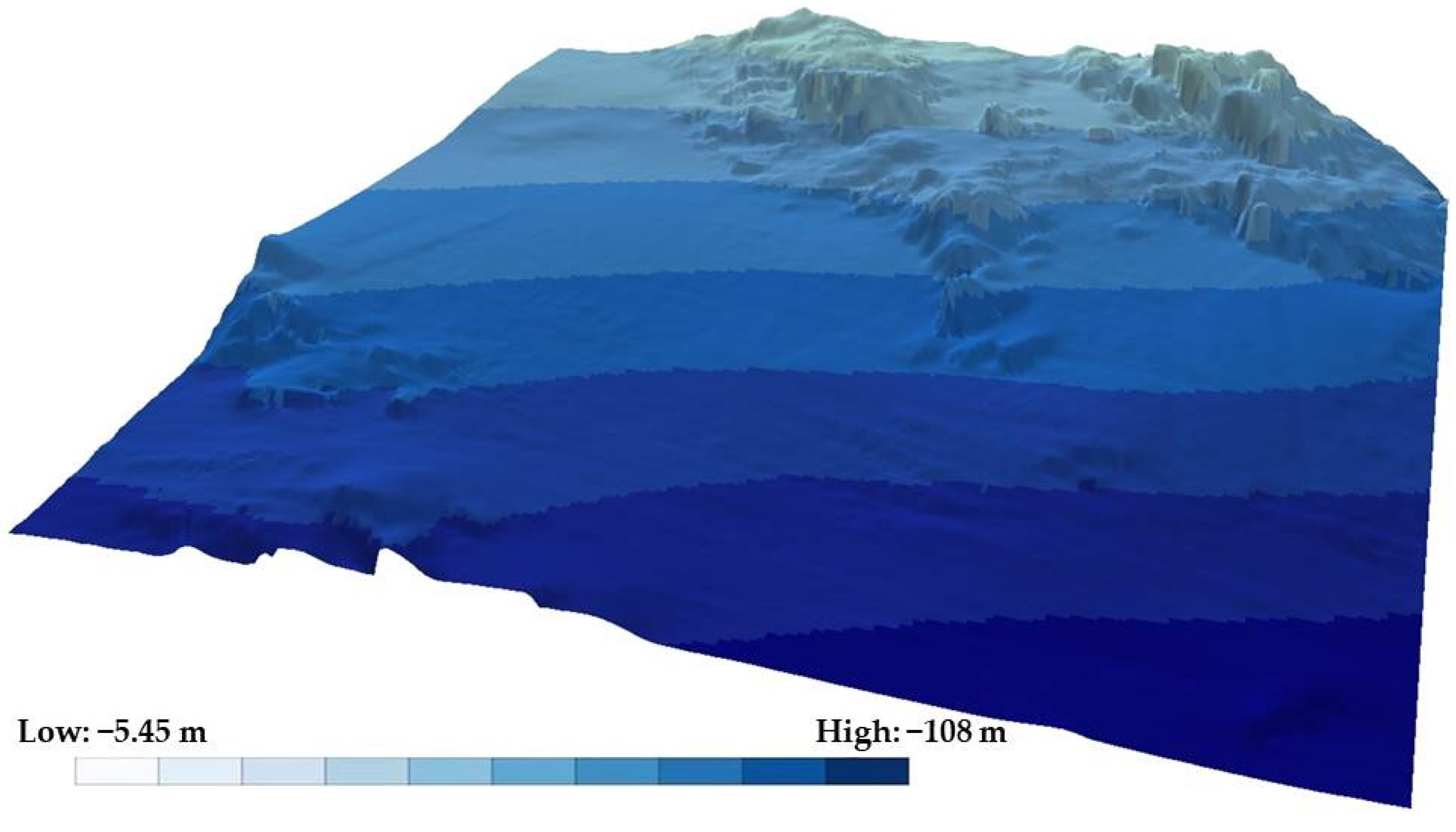
The statistical values obtained for sector B are always the most extreme: it has the highest maximum, standard deviation, and RMSE values, as well as the lowest minimum value. This is due to the particular conformation of this sector, which can be seen in detail in Figure 8. Nevertheless, the higher variability of sector B is remarked also by the MVI; starting from MBD, this index is calculated for all sectors to investigate the level of accuracy of the Kriging models related to the morphological aspects.
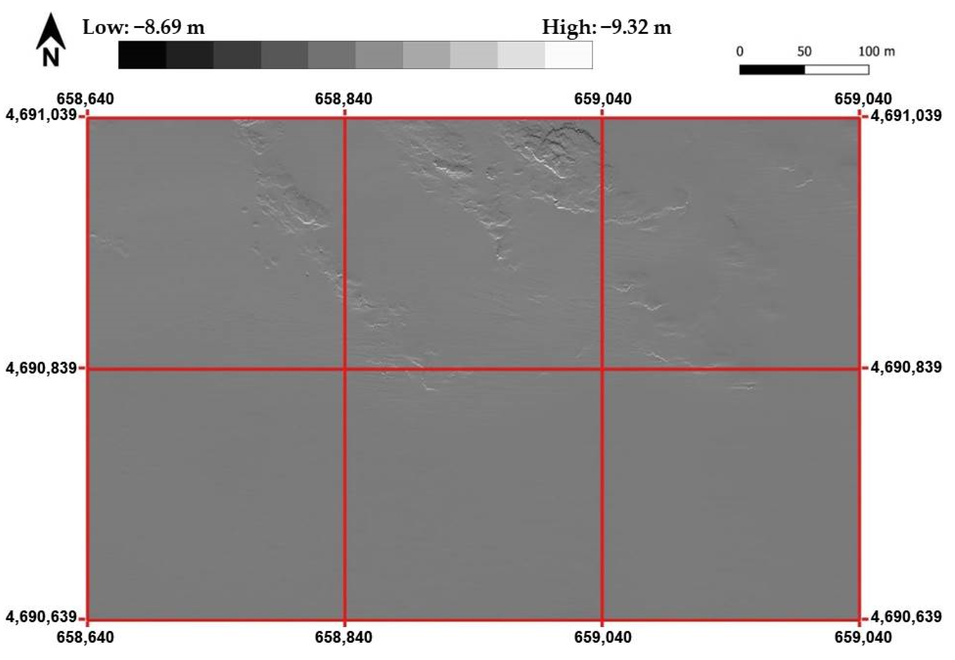
The calculation of the MVI was carried out in successive steps. In particular, the first step consisted of calculating the differences in the depth values of the pixels along x as well as along y, obtaining two images. The image related to the y direction is shown in Figure 9.
For the sake of completeness, the statistical values of the depth differences between successive pixels are reported in Table 7 (along x) and Table 8 (along y).
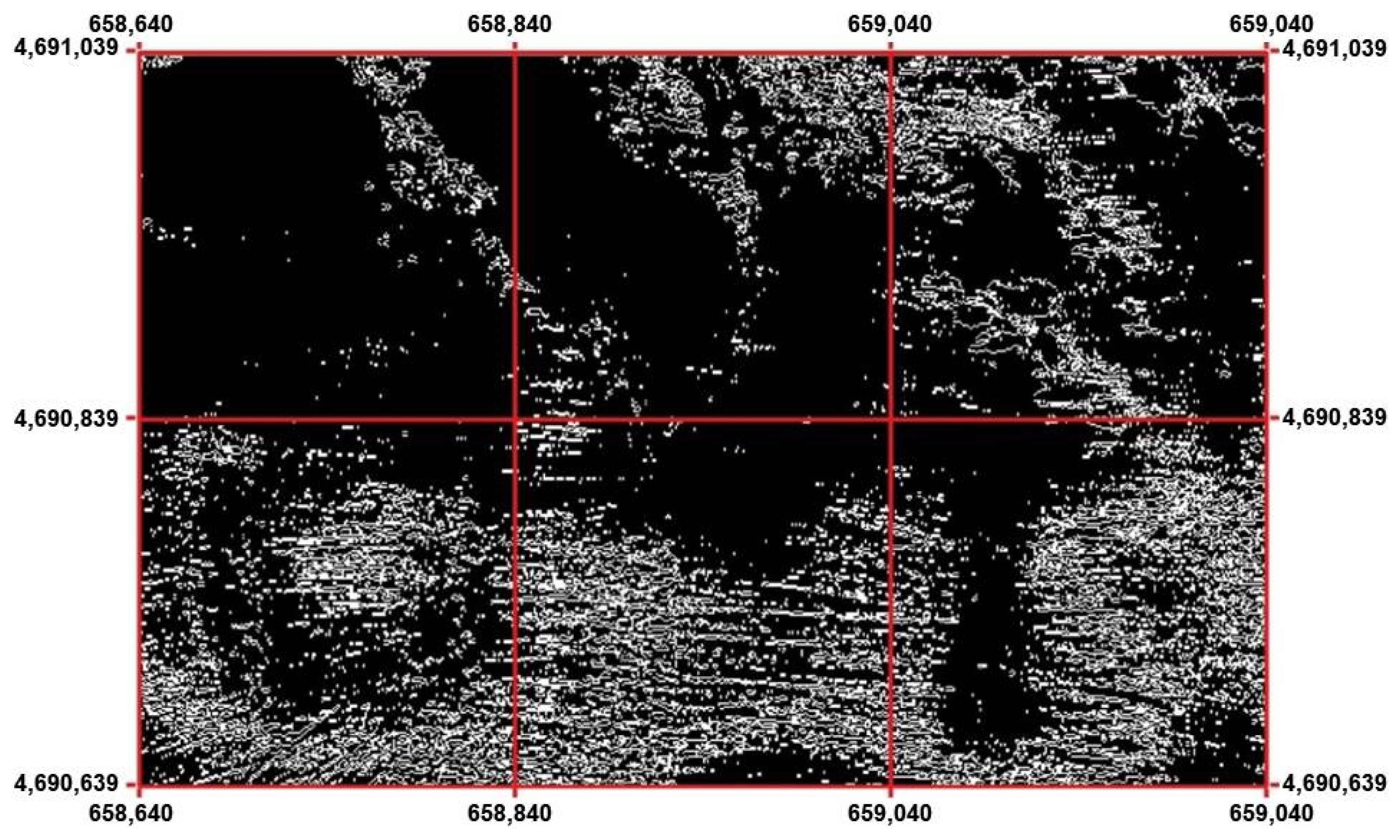
The second step analyzes the variability of the direction of the slope (ascending or descending) along the x and y directions; in particular the slope inversions between successive pixels are identified according to the procedure illustrated in Section 3.2.2. The image concerning the slope inversions along the y direction is shown in Figure 10.
Those raster files already provide an important indication for themself, namely the number of slope-reversals for each sector. Since the value 1 indicates the slope inversion and 0 the absence of variation, the mean value of all the pixels present in each sector was calculated as a parameter of the variability of the seabed. The two values calculated (one for the x direction and the other for the y direction) were used to achieve Ixy.
However, this is not enough for the purpose of studying the morphology of the seabed as an almost flat surface could still have many slope inversions, as in the case of sector D; in fact, in the neighboring pixels, they often have very similar depth values. Consequently other steps were necessary for determining the further parameter and Sxy was introduced in the MVI to take into account the level of inclination of the seabed and its variation. The study area has both low slope and steep slopes, often alternating with each other even at short distances, thus high values of abrupt variations were found.
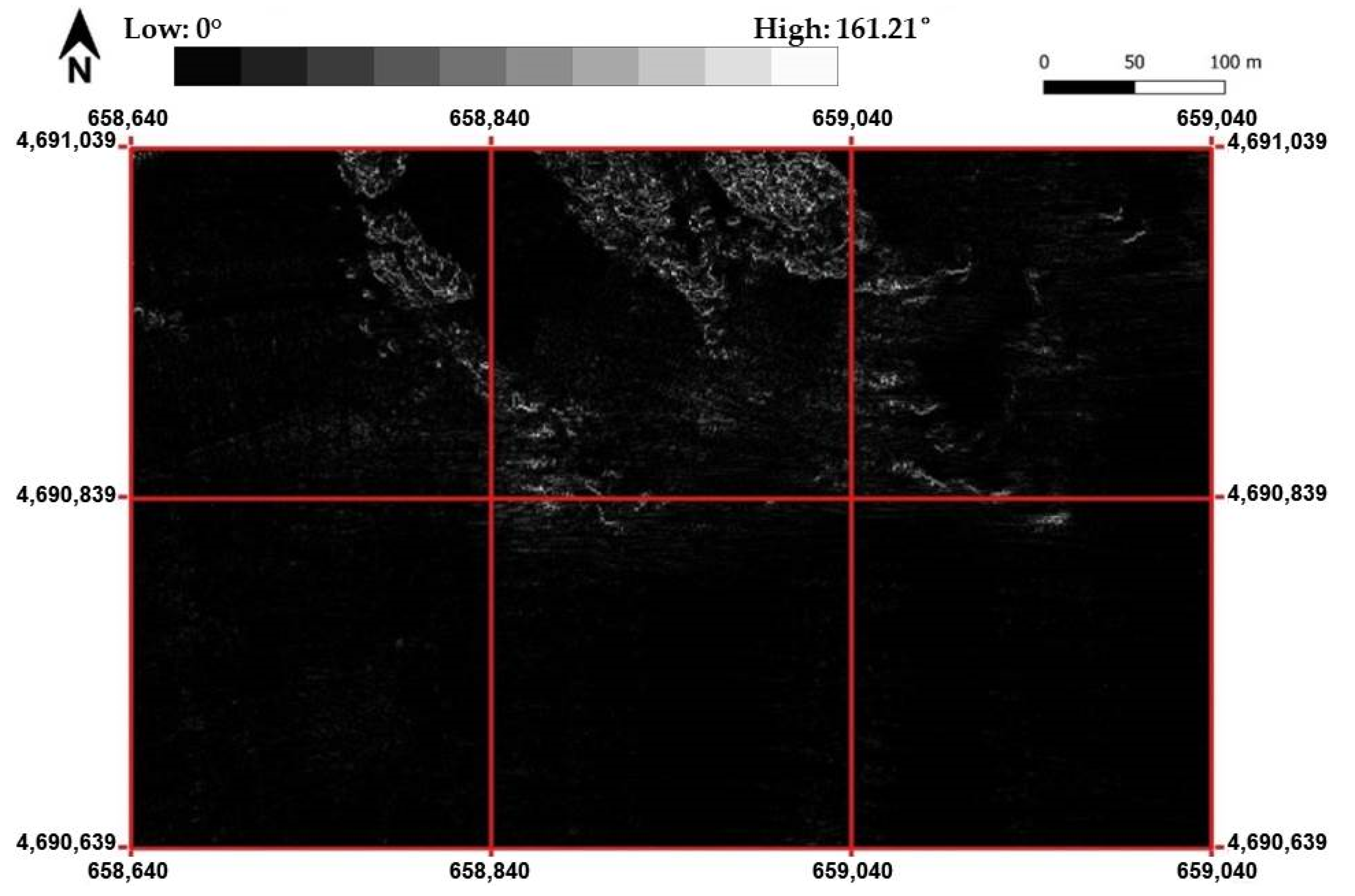
The third step involves calculating the variation of the slope along the x and y directions. Initially, using the raster calculator, the values of the depth difference between consecutive pixels were normalized with respect to the grid step size; the arctangent function applied to them provides the values of the slope in each pixel. Subsequently, in continuing to use the raster calculator, the variations of the slope between consecutive pixels were determined. The image concerning the slope variations along the y direction is shown in Figure 11.
These values were normalized by dividing by the theoretical maximum limit value of the slope variation (180°). In the end, we derived two images: the first relating to the slope variations along x and the other to the slope variations along y. The average of all the recorded values is Sxy.
From these values, the proposed index MVI was calculated according to Equation (15). The results are shown in Table 9.
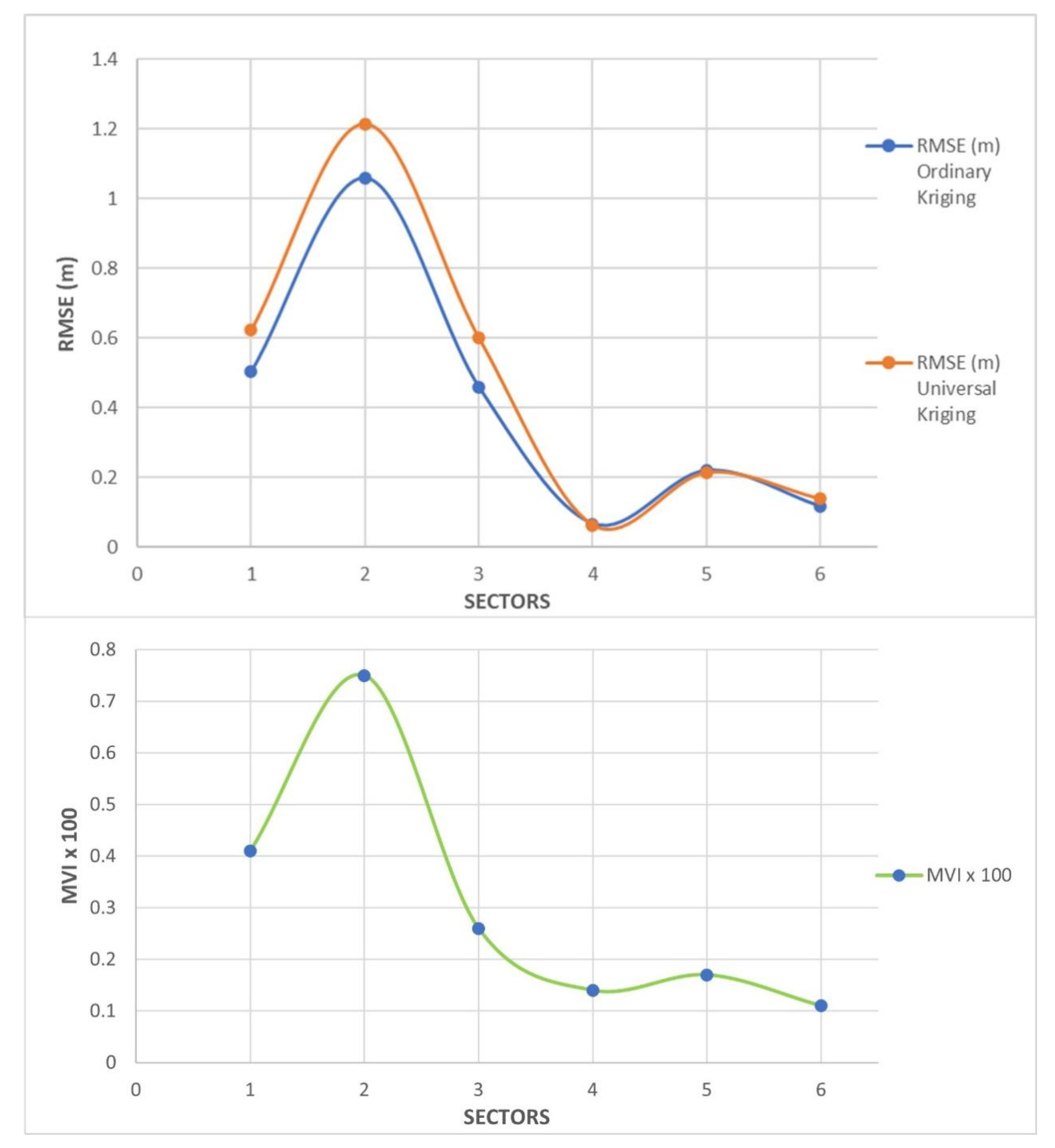
By comparing those values with the RMSE values, it is evident that, once the number of points to be interpolated is fixed, more accurate results are achieved in the presence of a low level of morphological variation. The Figure 12 highlights this aspect in the case of 2400 points.
At this point of our analysis, we wanted to reconsider the graphs shown in Figure 6 and Figure 7 in relation to the MVI indicator.
In the sectors where the lowest values of the indicator are recorded (sector D, E, and F), the RMSE values of the residuals decrease rapidly as the number of known points increases. A density equal to at least 1 point every 1000 m2 is sufficient to make the RMSE values fall below 1 m for both Ordinary Kriging and Universal Kriging. On the contrary, for the sectors where the MVI indicator has the highest values, the RMSE below 1 m is much higher. In sector B, characterized by the highest value of MVI, 1 point per 100 m2 is just enough to obtain an RMSE of approximately 1 m but only in the case of the Ordinary Kriging. In fact, in the case of Universal Kriging, the same concentration determines an RMSE value that remains higher than 1 m (RMSE = 1.214 m).
Finally, we wanted to remark that in the presence of a high MVI, even if RMSE is not higher than 1 m, residuals can reach considerable values in some points, as evidenced by the statistics in sector B, as shown in Table 5 (−14.037 m for Universal Kriging) and Table 6 (−14.469 m for Ordinary Kriging).

5. Conclusions

In the case of very varied seabed morphology, it is essential, for different purposes (e.g., safe navigation or geological studies), to have a detailed and accurate bathymetric model. To achieve these results, particular attention must be given to the interpolation algorithms used to reproduce 3D models, starting from a dataset consisting of a point cloud.
The results of our study validate the efficiency of the Kriging methods, remarking the influence of the dataset location and density on the 3D model accuracy in the case of the interpolation process. To investigate this relationship, a new index called MVI was introduced as a measurement of the level of variation of seabed morphology; this index results from the product of two components: the first component (Ixy) is related to the frequency of the variation of the slope direction (ascending or descending) and the second (Sxy) is associated to the variation of the value of the slope, both considered for the x direction as well as y direction.
The experiments demonstrate that by using Universal Kriging as well as Ordinary Kriging, a density equal to at least 1 point every 1000 m2 is sufficient to produce an accurate model in areas characterized by a low level of variation of seabed morphology (not only RMSE but also minimum and maximum values fall below 1 m). On the contrary, a density 10 times greater than that is necessary to produce an accurate model in areas characterized by a high level of variation of seabed morphology; in this case, even if the RMSE drops below 1 m, there may be strong differences between the predicted and observed depths in some places, thus a further increment of the measured points is required.
MVI is useful to represent the seabed variation as a unique value but to calculate it in an accurate way, the morphology must be already known. In our study, we have determined its value because a grid model derived by MB survey is already available. Consequently, we used it to establish the relationship between point density and model accuracy; if we want to define a priori the optimal number of depths to measure in an unknown area for a bathymetric survey, we can try to calculate MVI using information available, e.g., previous survey data and/or nautical charts even on a smaller scale. In this case, you must know that the calculated MVI is an approximate value and does not provide the exact photograph of reality, thus the advantage of using it may be limited.
Concerning the future developments of this work, further studies will be focused on the relationship between bathymetric point density and seabed model accuracy. In particular, other datasets representative of different seabed configurations will be considered both in terms of depth range (in the proposed study, depths not exceeding 108 m were analyzed) and in terms of the extension of the study area. Higher values of point density will be investigated to achieve better results also in roughness areas. In addition, further tests will be carried out to validate the efficiency of the proposed MVI to represent the variation of seabed morphology.
Author Contributions

C.P. conceived the article and designed the experiments; E.A. and P.P.A. conducted the bibliographic research; C.P. organized the data collection and supervised the applications; E.A. and P.P.A. carried out experiments on Kriging applications; C.P. designed the MVI; E.A. and P.P.A. carried out the accuracy tests; and all authors took part in the result analysis and in writing the paper. All authors have read and agreed to the published version of the manuscript.

Funding

This research study received no external funding.

Institutional Review Board Statement

Not applicable.

Informed Consent Statement

Not applicable.

Data Availability Statement

Not applicable.

Acknowledgments

We wish to thank the Italian Hydrographic Authority (Istituto Idrografico della Marina Militare) for providing the data. In particular, we would like to thank Lieutenant Luigi Carnevale and hydrographic surveyor Nunziante Langellotto for their valuable technical support in data handling.

Conflicts of Interest

The authors declare no conflict of interest.

References

  1. Monego, M.; Menin, A.; Fabris, M.; Achilli, V. 3D survey of Sarno Baths (Pompeii) by integrated geomatic methodologies. J. Cult. Herit. 2019, 40, 240–246. [Google Scholar] [CrossRef]
  2. Ebolese, D.; Lo Brutto, M.; Dardanelli, G. The integrated 3D survey for underground archaeological environment. Int. Arch. Photogramm. Remote Sens. Spat. Inf. Sci. 2019, XLII-2/W9, 311–317. [Google Scholar] [CrossRef] [Green Version]
  3. Aguilar, F.J.; Fernández, I.; Casanova, J.A.; Ramos, F.J.; Aguilar, M.A.; Blanco, J.L.; Moreno, J.C. 3D coastal monitoring from very dense UAV-Based photogrammetric point clouds. In Advances on Mechanics, Design Engineering and Manufacturing; Springer: Cham, Switzerland, 2017; pp. 879–887. [Google Scholar] [CrossRef]
  4. Masiero, A.; Tucci, G.; Conti, A.; Fiorini, L.; Vettore, A. Initial evaluation of the potential of smartphone stereo-vision in museum visits. Int. Arch. Photogramm. Remote Sens. Spat. Inf. Sci. 2019, XLII-2/W11, 837–842. [Google Scholar] [CrossRef] [Green Version]
  5. Pepe, M.; Costantino, D.; Alfio, V.S.; Zannotti, N. 4D geomatics monitoring of a quarry for the calculation of extracted volumes by tin and grid model: Contribute of UAV photogrammetry. Geogr. Tech. 2020, 16, 1–14. [Google Scholar] [CrossRef]
  6. Baiocchi, V.; Napoleoni, Q.; Tesei, M.; Servodio, G.; Alicandro, M.; Costantino, D. UAV for monitoring the settlement of a landfill. Eur. J. Remote Sens. 2019, 52 (Suppl. 3), 41–52. [Google Scholar] [CrossRef]
  7. Shingare, P.P.; Kale, S.S. Review on digital elevation model. Int. J. Mod. Eng. Res. 2013, 3, 2412–2418. [Google Scholar]
  8. Habib, M.; Alzubi, Y.; Malkawi, A.; Awwad, M. Impact of interpolation techniques on the accuracy of large-scale digital elevation model. Open Geosci. 2020, 12, 190–202. [Google Scholar] [CrossRef]
  9. Alcaras, E.; Carnevale, L.; Parente, C. Interpolating single-beam data for sea bottom GIS modelling. Int. J. Emerg. Trends Eng. Res. 2020, 8, 591–597. [Google Scholar] [CrossRef]
  10. Arun, P.V. A comparative analysis of different DEM interpolation methods. Egypt. J. Remote Sens. Space Sci. 2013, 16, 133–139. [Google Scholar] [CrossRef] [Green Version]
  11. Tobler, W.R. A computer movie simulating urban growth in the Detroit region. Econ. Geogr. 1970, 46, 234–240. [Google Scholar] [CrossRef]
  12. Waters, M.N. Spatial interpolation I, lecture 40. In NCGIA Core Curriculum, Technical Issues in GIS; University of California: Santa Barbara, CA, USA, 1989. [Google Scholar]
  13. Mitas, L.; Mitasova, H. Spatial interpolation. Geogr. Inf. Syst. Princ. Tech. Manag. Appl. 1999, 1, 481–492. [Google Scholar]
  14. Chang, T.J.; Wang, W.L. Spatial Analysis Using GIS to Study Performance of Highway Culvers in Ohio. In Pipelines 2008: Pipeline Asset Management: Maximizing Performance of Our Pipeline Infrastructure; ASCE: Reston, VA, USA, 2008; pp. 1–10. [Google Scholar] [CrossRef]
  15. Burrough, P.A.; McDonnell, R.A. Principles of Geographical Information Systems; Oxford University Press: New York, NY, USA, 1998; p. 190. [Google Scholar]
  16. Vansarochana, A.; Tripathi, N.K.; Clemente, R. Finding appropriate interpolation techniques for topographic surface generation for mudslide risk zonation. Geocarto Int. 2009, 24, 313–332. [Google Scholar] [CrossRef]
  17. Lam, N.S.N. Spatial interpolation methods: A review. Am. Cartogr. 1983, 10, 129–150. [Google Scholar] [CrossRef]
  18. GIS Resources Classification of Interpolation. GIS Resources. Available online: https://gisresources.com/classification-of-interpolation_2/ (accessed on 27 December 2021).
  19. ESRI, Deterministic Methods for Spatial Interpolation, ArcGIS Pro 2.9. Available online: https://pro.arcgis.com/en/pro-app/latest/help/analysis/geostatistical-analyst/deterministic-methods-for-spatial-interpolation.htm (accessed on 27 December 2021).
  20. Eberly, S.; Swall, J.; Holland, D.; Cox, B.; Baldridge, E. Developing Spatially Interpolated Surfaces and Estimating Uncertainty; United States Environmental Protection Agency: Washington, DC, USA, 2004; pp. 28–40. [Google Scholar]
  21. Bhattacharjee, S.; Mitra, P.; Ghosh, S.K. Spatial interpolation to predict missing attributes in GIS using semantic kriging. IEEE Trans. Geosci. Remote Sens. 2013, 52, 4771–4780. [Google Scholar] [CrossRef]
  22. ESRI. How Inverse Distance Weighted Interpolation Works. In ArcGIS Pro Help; ESRI: Redlands, CA, USA, 2021; Available online: https://pro.arcgis.com/en/pro-app/latest/help/analysis/geostatistical-analyst/how-inverse-distance-weighted-interpolation-works.htm (accessed on 27 December 2021).
  23. Childs, C. Interpolating surfaces in ArcGIS spatial analyst. ArcUser 2004, 3235, 32–35. [Google Scholar]
  24. Tabios, G.Q., III; Salas, J.D. A comparative analysis of techniques for spatial interpolation of precipitation 1. JAWRA J. Am. Water Resour. Assoc. 1985, 21, 365–380. [Google Scholar] [CrossRef]
  25. Xie, Y.; Chen, T.B.; Lei, M.; Yang, J.; Guo, Q.J.; Song, B.; Zhou, X.Y. Spatial distribution of soil heavy metal pollution estimated by different interpolation methods: Accuracy and uncertainty analysis. Chemosphere 2011, 82, 468–476. [Google Scholar] [CrossRef] [PubMed]
  26. Parente, C.; Vallario, A. Interpolation of Single Beam Echo Sounder Data for 3D Bathymetric Model. Int. J. Adv. Comput. Sci. Appl. 2019, 10, 6–13. [Google Scholar] [CrossRef]
  27. Erdogan, S. A comparision of interpolation methods for producing digital elevation models at the field scale. Earth Surf. Process. Landf. 2009, 34, 366–376. [Google Scholar] [CrossRef]
  28. Ouma, Y.O.; Owiti, T.; Kipkorir, E.; Kibiiy, J.; Tateishi, R. Multitemporal comparative analysis of TRMM-3B42 satellite-estimated rainfall with surface gauge data at basin scales: Daily, decadal and monthly evaluations. Int. J. Remote Sens. 2012, 33, 7662–7684. [Google Scholar] [CrossRef]
  29. Chilès, J.P.; Delfiner, P. Geostatistics: Modeling Spatial Uncertainty; John Wiley & Sons. Inc.: Hoboken, NJ, USA, 1999. [Google Scholar]
  30. Kristić, M.; Žuškin, S.; Brčić, D.; Valčić, S. Zone of confidence impact on cross track limit determination in ECDIS passage planning. J. Mar. Sci. Eng. 2020, 8, 566. [Google Scholar] [CrossRef]
  31. Latapy, A.; Héquette, A.; Pouvreau, N.; Weber, N.; Robin-Chanteloup, J.B. Mesoscale morphological changes of nearshore sand banks since the early 19th century, and their influence on coastal dynamics, Northern France. J. Mar. Sci. Eng. 2019, 7, 73. [Google Scholar] [CrossRef] [Green Version]
  32. Kågesten, G.; Fiorentino, D.; Baumgartner, F.; Zillén, L. How Do Continuous High-Resolution Models of Patchy Seabed Habitats Enhance Classification Schemes? Geosciences 2019, 9, 237. [Google Scholar] [CrossRef] [Green Version]
  33. Iacono, C.L.; Mateo, M.; Gràcia, E.; Guasch, L.; Carbonell, R.; Serrano, L.; Serrano, O.; Dañobeitia, J. Very high-resolution seismo-acoustic imaging of seagrass meadows (Mediterranean Sea): Implications for carbon sink estimates. Geophys. Res. Lett. 2008, 35, 1–5. [Google Scholar] [CrossRef]
  34. El-Hattab, A.I. Single beam bathymetric data modelling techniques for accurate maintenance dredging. Egypt. J. Remote Sens. Space Sci. 2014, 17, 189–195. [Google Scholar] [CrossRef] [Green Version]
  35. Specht, M.; Specht, C.; Mindykowski, J.; Dabrowski, P.; Masnicki, R.; Makar, A. Geospatial Modeling of the Tombolo Phenomenon in Sopot using Integrated Geodetic and Hydrographic Measurement Methods. Remote Sens. 2020, 12, 737. [Google Scholar] [CrossRef] [Green Version]
  36. Sinapi, L.; Lamberti, L.O.; Pizzeghello, N.M.; Ivaldi, R. The Graham Bank: Hydrographic features and safety of navigation. Int. Hydrogr. Rev. 2016, 15, 7–20. [Google Scholar]
  37. Arseni, M.; Voiculescu, M.; Georgescu, L.P.; Iticescu, C.; Rosu, A. Testing different interpolation methods based on single beam echosounder river surveying. Case study: Siret River. ISPRS Int. J. Geo-Inf. 2019, 8, 507. [Google Scholar] [CrossRef] [Green Version]
  38. Wilson, M.F.; O’Connell, B.; Brown, C.; Guinan, J.C.; Grehan, A.J. Multiscale terrain analysis of multibeam bathymetry data for habitat mapping on the continental slope. Mar. Geod. 2007, 30, 3–35. [Google Scholar] [CrossRef] [Green Version]
  39. Degraer, S.; Moerkerke, G.; Rabaut, M.; Van Hoey, G.; Du Four, I.; Vincx, M.; Henriet, J.-P.; Van Lancker, V. Very-high resolution side-scan sonar mapping of biogenic reefs of the tube-worm Lanice conchilega. Remote Sens. Environ. 2008, 112, 3323–3328. [Google Scholar] [CrossRef]
  40. Wang, L.; Liu, H.; Su, H.; Wang, J. Bathymetry retrieval from optical images with spatially distributed support vector machines. GIScience Remote Sens. 2019, 56, 323–337. [Google Scholar] [CrossRef]
  41. Liu, Y.; Wu, Z.; Zhao, D.; Zhou, J.; Shang, J.; Wang, M.; Zhu, C.; Luo, X. Construction of high-resolution bathymetric dataset for the Mariana Trench. IEEE Access 2019, 7, 142441–142450. [Google Scholar] [CrossRef]
  42. Flemming, B.W. Side-scan sonar: A practical guide. Int. Hydrogr. Rev. 1976, 53, 65–92. [Google Scholar]
  43. Ceylan, A.; Karabork, H.; Ekozoglu, I. An analysis of bathymetric changes in Altinapa reservoir. Carpathian J. Earth Environ. Sci. 2011, 6, 15–24. [Google Scholar]
  44. Stumpf, R.P.; Holderied, K.; Sinclair, M. Determination of water depth with high-resolution satellite imagery over variable bottom types. Limnol. Oceanogr. 2003, 48, 547–556. [Google Scholar] [CrossRef]
  45. Parente, C.; Pepe, M. Bathymetry from worldView-3 satellite data using radiometric band ratio. Acta Polytech. 2018, 58, 109–117. [Google Scholar] [CrossRef] [Green Version]
  46. Carrara, A.; Bitelli, G.; Carla, R. Comparison of techniques for generating digital terrain models from contour lines. Int. J. Geogr. Inf. Sci. 1997, 11, 451–473. [Google Scholar] [CrossRef]
  47. Chung, J.W.; Rogers, J.D. Interpolations of groundwater table elevation in dissected uplands. Groundwater 2012, 50, 598–607. [Google Scholar] [CrossRef]
  48. Sassais, R.; Makar, A. Methods to generate numerical models of terrain for spatial ENC presentation. Annu. Navig. 2011, 18, 69–81. [Google Scholar]
  49. Gosciewski, D. The effect of the distribution of measurement points around the node on the accuracy of interpolation of the digital terrain model. J. Geogr. Syst. 2013, 15, 513–535. [Google Scholar] [CrossRef] [Green Version]
  50. Mesa-Mingorance, J.L.; Ariza-López, F.J. Accuracy assessment of digital elevation models (DEMs): A critical review of practices of the past three decades. Remote Sens. 2020, 12, 2630. [Google Scholar] [CrossRef]
  51. Aguilar Torres, F.J.; Aguilar Torres, M.A.; Agüera Vega, F.; Carvajal Ramírez, F.; Sánchez Salmerón, P.L. Efectos de la Morfología del Terreno, Densidad Muestral y Métodos de Interpolación en la Calidad de los Modelos Digitales de Elevaciones. In Proceedings of the XIV Congreso Internacional de Ingeniería Gráfica, INGEGRAF, Santander, Spain, 5–7 June 2002. [Google Scholar]
  52. Bakuła, K. Reduction of DTM obtained from LiDAR data for flood modeling. Arch. Fotogram. Kartogr. I Teledetekcji 2011, 22, 51–61. [Google Scholar]
  53. Stereńczak, K.; Ciesielski, M.; Balazy, R.; Zawiła-Niedźwiecki, T. Comparison of various algorithms for DTM interpolation from LIDAR data in dense mountain forests. Eur. J. Remote Sens. 2016, 49, 599–621. [Google Scholar] [CrossRef]
  54. Zhang, Z.; Gerke, M.; Vosselman, G.; Yang, M.Y. Filtering photogrammetric point clouds using standard LiDAR filters towards DTM generation. ISPRS Ann. Photogramm. Remote Sens. Spat. Inf. Sci. 2018, IV-2, 319–326. [Google Scholar] [CrossRef] [Green Version]
  55. Aguilar, F.J.; Agüera, F.; Aguilar, M.A.; Carvajal, F. Effects of terrain morphology, sampling density, and interpolation methods on grid DEM accuracy. Photogramm. Eng. Remote Sens. 2005, 71, 805–816. [Google Scholar] [CrossRef] [Green Version]
  56. Chaplot, V.; Darboux, F.; Bourennane, H.; Leguédois, S.; Silvera, N.; Phachomphon, K. Accuracy of interpolation techniques for the derivation of digital elevation models in relation to landform types and data density. Geomorphology 2006, 77, 126–141. [Google Scholar] [CrossRef]
  57. Dupuy, R.; Makar, A. Analysis of digital sea bottom models generated using ENC data. Annu. Navig. 2011, 18, 27–36. [Google Scholar]
  58. Alcaras, E.; Parente, C.; Vallario, A. A Comparison of different interpolation methods for DEM production. Int. J. Adv. Trends Comput. Sci. Eng. 2019, 6, 1654–1659. [Google Scholar] [CrossRef]
  59. Cutroneo, L.; Ferretti, G.; Scafidi, D.; Ardizzone, G.D.; Vagge, G.; Capello, M. Current observations from a looking down vertical V-ADCP: Interaction with winds and tide? The case of Giglio Island (Tyrrhenian Sea, Italy). Oceanologia 2017, 59, 139–152. [Google Scholar] [CrossRef]
  60. Frezza, V.; Carboni, M.G. Distribution of recent foraminiferal assemblages near the Ombrone River mouth (Northern Tyrrhenian Sea, Italy). Rev. Micropaléontologie 2009, 52, 43–66. [Google Scholar] [CrossRef]
  61. ESRI (Environmental Systems Research Institute). ArcGIS 10.3; ESRI: Redlands, CA, USA, 2012. [Google Scholar]
  62. ESRI (Environmental Systems Research Institute). Geostatistical Analyst, ArcGIS 10.3; ESRI: Redlands, CA, USA, 2012. [Google Scholar]
  63. Efron, B. The Jackknife, the Bootstrap and other resampling plans. In CBMS-NSF Regional Conference Series in Applied Mathematics; Society for Industrial and Applied Mathematics (SIAM): Philadelphia, PA, USA, 1982. [Google Scholar]
  64. Krivoruchko, K. Empirical bayesian Kriging-Implemented in ArcGIS Geostatistical Analyst. ArcUser Fall 2012, 6, 1–5. [Google Scholar]
  65. Ceron, W.L.; Andreoli, R.V.; Kayano, M.T.; Canchala, T.; Carvajal-Escobar, Y.; Souza, R.A. Comparison of spatial interpolation methods for annual and seasonal rainfall in two hotspots of biodiversity in South America. An. Acad. Bras. Ciências 2021, 93, e20190674. [Google Scholar] [CrossRef] [PubMed]
  66. Salekin, S.; Burgess, J.H.; Morgenroth, J.; Mason, E.G.; Meason, D.F. A comparative study of three non-geostatistical methods for optimising digital elevation model interpolation. ISPRS Int. J. Geo-Inf. 2018, 7, 300. [Google Scholar] [CrossRef] [Green Version]
  67. Gentilucci, M.; Barbieri, M.; Burt, P.; D’Aprile, F. Preliminary data validation and reconstruction of temperature and precipitation in Central Italy. Geosciences 2018, 8, 202. [Google Scholar] [CrossRef] [Green Version]
  68. Bargaoui, Z.K.; Chebbi, A. Comparison of two Kriging interpolation methods applied to spatiotemporal rainfall. J. Hydrol. 2009, 365, 56–73. [Google Scholar] [CrossRef]
  69. Wu, T.; Li, Y. Spatial interpolation of temperature in the United States using residual Kriging. Appl. Geogr. 2013, 44, 112–120. [Google Scholar] [CrossRef]
  70. Robinson, T.P.; Metternicht, G. A comparison of inverse distance weighting and Ordinary Kriging for characterising within-paddock spatial variability of soil properties in Western Australia. Cartography 2003, 32, 11–24. [Google Scholar] [CrossRef]
  71. Alcaras, E.; Falchi, U.; Parente, C. Digital Terrain Model Generalization for Multiscale Use. Int. Rev. Civ. Eng. (IRECE) 2020, 11, 52–59. [Google Scholar] [CrossRef]
  72. Stein, M.L. Interpolation of Spatial Data: Some Theory for Kriging; Springer Science & Business Media: Berlin/Heidelberg, Germany, 1999. [Google Scholar]
  73. Jian, X.; Olea, R.A.; Yu, Y.S. Semivariogram modeling by weighted least squares. Comput. Geosci. 1996, 22, 387–397. [Google Scholar] [CrossRef]
  74. Rishikeshan, C.A.; Katiyar, S.K.; Mahesh, V.V. Detailed evaluation of DEM interpolation methods in GIS using DGPS data. In Proceedings of the 2014 International Conference on Computational Intelligence and Communication Networks, Bhopal, India, 14–16 November 2014; IEEE: Hoboken, NJ, USA; pp. 666–671. [Google Scholar] [CrossRef]
  75. Malvić, T.; Ivšinović, J.; Velić, J.; Rajić, R. Kriging with a small number of data points supported by Jack-Knifing, a case study in the Sava depression (Northern Croatia). Geosciences 2019, 9, 36. [Google Scholar] [CrossRef] [Green Version]
  76. Kiš, I.M. Comparison of Ordinary and Universal Kriging interpolation techniques on a depth variable (a case of linear spatial trend), case study of the Šandrovac Field. Rud.-Geološko-Naft. Zb. (Min.-Geol.-Pet. Bull.) 2016, 31, 41–58. [Google Scholar] [CrossRef]
  77. Wackernagel, H. Ordinary Kriging. In Multivariate Geostatistics; Springer: Berlin/Heidelberg, Germany, 2003; pp. 79–88. [Google Scholar] [CrossRef]
  78. Webster, R.; Oliver, M.A. Geostatistics for Environmental Scientists; John Wiley & Sons: Chichester, UK, 2007. [Google Scholar]
  79. ESRI. Understanding Ordinary Kriging, ArcGIS 10.3- Help, Redlands, CA, USA. Available online: http://webhelp.esri.com/arcgisdesktop/9.2/index.cfm?TopicName=Understanding_Ordinary_Kriging (accessed on 26 December 2021).
  80. ILWIS (The Integrated Land and Water Information System) Team. ILWI Software 3.5—Help; Faculty of Geo-Information Science and Earth Observation: Enschede, The Netherlands, 2008. [Google Scholar]
  81. Kumar, V. Optimal contour mapping of groundwater levels using Universal Kriging—A case study. Hydrol. Sci. J. 2007, 52, 1038–1050. [Google Scholar] [CrossRef]
  82. ESRI. Understanding Universal Kriging, ArcGIS 10.3- Help, Redlands, CA, USA. Available online: https://desktop.arcgis.com/en/arcmap/latest/extensions/geostatistical-analyst/understanding-Universal-Kriging.htm (accessed on 26 December 2021).
  83. Johnston, K.; Ver Hoef, J.M.; Krivoruchko, K.; Lucas, N. Using ArcGIS Geostatistical Analyst; Esri: Redlands, CA, USA, 2001; Volume 380. [Google Scholar]
  84. Falchi, U.; Parente, C.; Prezioso, G. Global geoid adjustment on local area for GIS applications using GNSS permanent station coordinates. Geod. Cartogr. 2018, 44, 80–88. [Google Scholar] [CrossRef] [Green Version]
  85. Xiao, Y.; Gu, X.; Yin, S.; Shao, J.; Cui, Y.; Zhang, Q.; Niu, Y. Geostatistical interpolation model selection based on ArcGIS and spatio-temporal variability analysis of groundwater level in piedmont plains, Northwest China. SpringerPlus 2016, 5, 425. [Google Scholar] [CrossRef] [Green Version]
  86. Sain, S.R.; Baggerly, K.A.; Scott, D.W. Cross-validation of multivariate densities. J. Am. Stat. Assoc. 1994, 89, 807–817. [Google Scholar] [CrossRef]
  87. Browne, M.W. Cross-validation methods. J. Math. Psychol. 2000, 44, 108–132. [Google Scholar] [CrossRef] [Green Version]
  88. Refaeilzadeh, P.; Tang, L.; Liu, H. Cross-validation. Encycl. Database Syst. 2009, 5, 532–538. [Google Scholar] [CrossRef]
  89. Lam, K.C.; Bryant, R.G.; Wainright, J. Application of spatial interpolation method for estimating the spatial variability of rainfall in semiarid New Mexico, USA. Mediterr. J. Soc. Sci. 2015, 6, 108. [Google Scholar] [CrossRef] [Green Version]
  90. Berrar, D. Cross-Validation. Encycl. Bioinform. Comput. Biol. 2019, 1, 542–545. [Google Scholar] [CrossRef]
  91. Fasshauer, G.E.; Zhang, J.G. On choosing “optimal” shape parameters for RBF approximation. Numer. Algorithms 2007, 45, 345–368. [Google Scholar] [CrossRef]
  92. Tomlin, C.D. Map algebra: One perspective. Landsc. Urban Plan. 1994, 30, 3–12. [Google Scholar] [CrossRef]
  93. Li, Z. On the measure of digital terrain model accuracy. Photogramm. Rec. 1988, 12, 873–877. [Google Scholar] [CrossRef]
  94. Yang, X.; Hodler, T. Visual and statistical comparisons of surface modeling techniques for point-based environmental data. Cartogr. Geogr. Inf. Sci. 2000, 27, 165–175. [Google Scholar] [CrossRef]
  95. Lozano Parra, F.J.; Gutiérrez, Á.G.; Fernández, M.P.; Contador, J.L. Classification of morphometric units from digital terrain models: Applications in land cover classification. Rocz. Geomatyki 2009, 7, 83–89. [Google Scholar]
  96. ESRI. How Slope Works, Spatial-Analyst-Toolbox. ArcGIS. Available online: https://desktop.arcgis.com/en/arcmap/10.3/tools/spatial-analyst-toolbox/how-slope-works.htm (accessed on 26 December 2021).
  97. Zevenbergen, L.W.; Thorne, C.R. Quantitative analysis of land surfacetopography. Earth Surf. Processes Landf. 1987, 12, 47–56. [Google Scholar] [CrossRef]
  98. Wu, J.; Fang, J.; Tian, J. Terrain Representation and Distinguishing Ability of Roughness Algorithms Based on DEM with Different Resolutions. ISPRS Int. J. Geo-Inf. 2019, 8, 180. [Google Scholar] [CrossRef] [Green Version]
  99. Riley, S.J.; DeGloria, S.D.; Elliot, R. Index that quantifies topographic heterogeneity. Intermt. J. Sci. 1999, 5, 23–27. [Google Scholar]
Figure 1. Three-dimensional representation of the seafloor obtained from the entire multi-beam dataset (MBD): the upper image represents the point cloud of the initial MBD; the lower image represents the continuous 3D model of the seafloor.
Geosciences 12 00062 g001
Figure 2. The study area: on the left, localization of Giglio Island into Tyrrhenian Sea, in equirectangular projection and WGS84 geographic coordinates (EPSG: 4326); on the right, Giglio Island visualization in RGB composition of Sentinel-2B images in UTM/WGS 84 plane coordinates expressed in meters (EPSG: 32632), with the study area highlighted in the red rectangle.
Geosciences 12 00062 g002
Figure 3. The study area with 2400 chosen points (in red) in UTM/WSG 84 plane coordinates expressed in meters (EPSG: 32632).
Geosciences 12 00062 g003
Figure 4. Slopes chart of the initial MBD in UTM/WSG 84 plane coordinates expressed in meters (EPSG: 32632).
Geosciences 12 00062 g004
Figure 5. Division of the study area into 6 sectors (AF), each of 200 m on each side.
Geosciences 12 00062 g005
Figure 6. Direct comparison of Ordinary Kriging models with MBD: the variation of RMSE related to the number of points analyzed in each sector.
Geosciences 12 00062 g006
Figure 7. Direct comparison of Universal Kriging models with MBD: the variation of RMSE related to the number of points analyzed in each sector.
Geosciences 12 00062 g007
Figure 8. Three-dimensional representation of the seafloor in sector B. The detail permits us to appreciate the high variability of the seafloor.
Geosciences 12 00062 g008
Figure 9. Image of the differences of MBD values along y direction.
Geosciences 12 00062 g009
Figure 10. The image of the slope inversions along y direction in the study area (the pixels in which slope inversions occur are colored white).
Geosciences 12 00062 g010
Figure 11. The slope variations (in degree) along y direction.
Geosciences 12 00062 g011
Figure 12. RMSE values in the case of 2400 points using Ordinary Kriging and Universal Kriging for each sector (upper) and MVI values calculated in the six sectors (lower).
Geosciences 12 00062 g012
Table 1. Statistical terms of the residuals supplied by cross-validation for the Ordinary Kriging.
CountMin (m)Max (m)Mean (m)St. Dev. (m)RMSE (m)
24−13.49511.618−0.3034.4794.489
48−12.5878.4870.1393.0143.017
120−9.8955.095−0.1341.8921.897
240−9.06211.159−0.0421.3311.332
480−8.8108.2110.0211.1301.130
1200−7.3665.3050.0020.7140.714
2400−5.9454.760−0.0020.5030.503
Table 2. Statistical terms of the residuals between each Ordinary Kriging model and initial dataset values.
CountMin (m)Max (m)Mean (m)St. Dev. (m)RMSE (m)
24−30.7996.526−0.2134.0474.053
48−17.09811.578−0.1802.0522.060
120−12.33721.0970.0562.0202.020
240−10.69410.399−0.1101.3441.349
480−11.4577.816−0.0591.0871.089
1200−8.0677.7030.0070.6630.663
2400−14.0377.720−0.0080.5370.537
Table 3. Statistical terms of the residuals supplied by cross-validation for the Universal Kriging.
CountMin (m)Max (m)Mean (m)St. Dev. (m)RMSE (m)
24−14.74512.489−0.2335.1005.105
48−16.0028.574−0.2973.2973.310
120−15.21210.861−0.0172.1682.168
240−11.03211.916−0.0131.5811.581
480−11.1887.590−0.0411.2111.212
1200−6.7994.8300.0060.7520.752
2400−8.3075.835−0.0030.6280.628
Table 4. Statistical terms of the residuals between each Universal Kriging model and initial dataset values.
CountMin (m)Max (m)Mean (m)St. Dev. (m)RMSE (m)
24−32.56310.076−0.3404.8514.863
48−24.20121.304−0.3213.4593.474
120−15.36031.6170.0982.3192.321
240−12.15417.509−0.1081.5661.570
480−12.32017.700−0.0061.1801.180
1200−15.7958.5320.0130.7950.795
2400−17.1518.575−0.0160.6460.647
Table 5. Statistical terms of the residuals between the Ordinary Kriging model with 2400 total points and initial dataset values for B and D sectors.
SectorMin (m)Max (m)Mean (m)St. Dev. (m)RMSE (m)
B−14.0377.720−0.0151.0611.061
D−0.4050.352−0.0030.0670.067
Table 6. Statistical terms of the residuals between the Universal Kriging model with 2400 total points and initial dataset values for B and D sectors.
SectorMin (m)Max (m)Mean (m)St. Dev. (m)RMSE (m)
B−14.4697.499−0.0461.2141.214
D−0.4860.353−0.0010.0640.064
Table 7. Statistical terms of the differences of MBD values along x direction.
SectorMin (m)Max (m)Mean (m)St. Dev. (m)
A−5.2506.540−0.0410.260
B−8.0309.050−0.0910.503
C−5.2803.890−0.2000.242
D−0.4400.270−0.0910.040
E−2.8104.240−0.0690.090
F−2.6702.310−0.0680.063
Table 8. Statistical terms of the differences of MBD values along y direction.
SectorMin (m)Max (m)Mean (m)St. Dev. (m)
A−4.5707.8300.2580.287
B−8.6909.3200.2870.552
C−3.0204.2800.1050.254
D−0.2800.4200.0330.055
E−1.8304.4900.0500.138
F−1.5103.3300.0170.089
Table 9. Morphological variation index (MVI) achieved for each sector.
SectorMVI
A0.0041
B0.0075
C0.0026
D0.0014
E0.0017
F0.0011
Publisher’s Note: MDPI stays neutral with regard to jurisdictional claims in published maps and institutional affiliations.