A Tool for Performing Automatic Kinematic Analysis on Rock Outcrops

Abstract

The assessment of rock outcrops’ predisposition to the main possible kinematisms represents the preliminary step of stability analysis: Markland’s tests for sliding and toppling constitute a milestone due to the ease of use and interpretation of results. Orientation and friction angles of the main discontinuity sets and orientation of rock faces are required as input to perform the test on a stereonet graphically. However, for natural outcrops, the orientation of rock faces could vary significantly, and the test should be performed assuming all the representative ones. To speed up this process, the authors set up an automatic procedure based on the GIS environment working principles and developed it in Matlab language. Main discontinuity sets orientation and relative friction angles, along with slope and aspect data representing the rockface orientation of the considered outcrop, are the input data. The slope and aspect data are in GeoTIFF format, the most common format for georeferenced raster files employed in a GIS environment. The Matlab code performs Markland’s tests for planar and wedge sliding and flexural toppling, considering all the possible sets or intersections of sets, and provides the output with the same extent and georeferencing of the input data. The outputs are a series of GeoTIFF raster files describing the result for each kinematism separately and globally, which can be imported directly into GIS. The global results can also be used to map source areas for 3D rockfall numerical simulations. The code was validated through a case study by comparing its results with those obtained by performing the conventional tests singularly on a number of significant rock faces. The results obtained in the case study show that the algorithm produces reliable results consistent with those provided by traditional methods.

1. Introduction

When dealing with instability involving rock masses and rock faces, the first step usually consists of the analysis of those movements that are actually possible given the features of the rock mass itself. This corresponds to carrying out a kinematic analysis of the rock mass, which compares from the geometrical point of view the orientation of the rockface and that of the discontinuity sets of the rock mass. The orientation is expressed through a pair of angular values representing the dip and dip direction [1]. A representative friction angle value for each of the joint sets completes the rock mass description. These parameters are then employed to establish which among the three possible types of movements are geometrically possible: planar sliding (PS), wedge sliding (WS), and toppling (TP).

The most common approach consists in performing the so-called Markland’s tests [2,3], usually with the help of stereoplots: for each of the three types of movement, a series of thresholds are set to define which joint set can produce it with reference to the considered rockface. This process involves, though, a certain degree of simplification. In its simplest form, these tests are performed using dip and dip direction reference values for both the joint sets and the rockface, usually chosen as average values after performing an initial analysis on numerous data sets. This approach, sometimes indicated as deterministic [4,5], simplifies the procedure but is effective only in peculiar situations: on the one hand, when the joint sets are clearly defined and with low dispersion of the actual dip and dip direction values, and on the other hand when the rockface is geometrically simple and regular, so that a single orientation may describe it with sufficient precision. It is needless to say that these kinds of scenarios are not unrealistic, but uncommon at least, even if it is possible to replicate these conditions by dividing a rock face into a reasonable number of homogeneous domains. This operation, though, has the inconvenient consequence of increasing the number of times the kinematic tests must be performed.

The literature also suggests [4,5] a probabilistic approach, which completely avoids the need to define the average orientation for each set by directly employing the raw data acquired during the survey. A similar challenge in defining a reference orientation arises when dealing with articulated or complex rockfaces. The researchers began more than 20 years ago to focus on the effectiveness of employing Digital Terrain Models (DTM) or Digital Surface Models (DSM) [6,7,8,9], given that DTMs were already used in modeling slope stability since the mid-80s [10,11]. Using a DTM or a DSM to reproduce the geometry of a rockface has two major advantages:

-

A DTM represents the surface of the slope or rockface. It allows overcoming the need to simplify the rockface into homogeneous domains based on their orientation;

-

A DTM is a 3D map; therefore, it enables locating the results of the tests obtained from the stereoplots interpretation.

Basically, the kinematic tests could be run in every cell of the DTM as if dividing the rockface into a huge number of homogeneous domains: an absolutely impractical approach without computer technology. The limits of the use of DTMs or DSMs are mostly confined to their accuracy and spatial resolution, which, however, in the last years, have been greatly improved by technologies such as drone-based photogrammetry and LiDAR techniques. Another issue that most likely marked the unsuccessful diffusion of this kind of approach when it was first introduced before the year 2000 is related to the limits of computer technology in aspects such as computational power and memory storage in commercial machines. A highly detailed DSM, such as those produced currently, would have been completely inaccessible and unemployable by computers just a decade ago.

The authors of this paper produced an algorithm that performs kinematic analysis employing as input data only a DTM of the rockface and sufficient knowledge of the rock mass joints orientation to define reference values for each of the considered joint sets. The aim is to provide a tool that could avoid the repetition of manual tasks, such as those involved in the traditional approach, and significantly speed up the process. In order to do so, some requirements need to be met: first of all, a precise and detailed survey of the rock face and the surrounding area is required; secondly, the rock mass discontinuities have to be described by a reasonable amount of orientation measures, either measured on outcrops or the rock mass directly or by non-contact methods; and lastly, a DEM or DSM needs to be provided ad hoc, with resolution and precision coherent to those expected in the results. Once these three sine qua non conditions are met, the process is linear and simple. The algorithm is based on two widespread platforms: QGis for the mapping part and Matlab for the actual processing of the input data. Previously, other authors employed similar instruments but tried to achieve either susceptibility or stability mapping, resulting in more complex approaches involving more sophisticated techniques such as probabilistic methods [7,12], proper stability evaluations [13], or machine learning [14]. It is quite common to find in the literature authors who use DTM to identify source areas for landslides or, specifically, rockfall [15,16]: generally, these methods analyze morphometric parameters, such as slope angle or surface curvature, setting a threshold value, and in this way defining what should be considered a source area. Some authors use the DTM to perform kinematic analyses, but not with an automatic process [17,18], or approach the problem by identifying potentially unstable blocks first and then using the DTM to model them [19,20]. There also exist some methods and approaches that employ point clouds instead of DTMs or DSMs [21,22]. A point cloud can represent the rockface with high or very high resolution even when the dip is equal to 90° or even reversed: something a DTM, by definition, cannot do, given its 2.5D geometry. This, though, requires costlier input data, such as laser scanner surveys, and a much more complex process.

The algorithm presented here is a straightforward solution to identify positions on a rockface or slope where Markland’s tests for the three main types of movement give a positive response and map them. This is achieved by coupling the QGis 3.16 and Matlab R2022a environments: by employing a geographic information system (GIS) it is possible to store the geographic data associated with the DTM input, while in Matlab, it is possible to write a code to automatically perform the numerical evaluations. Theoretically, it is possible to complete all the operations involved in this algorithm in QGis or any other GIS platform, either by hand or with some limited form of automation; this corresponds to a highly time-consuming process prone to errors. For this reason, the authors chose to couple QGis with Matlab so that the process can be shortened significantly and streamlined. The coupling requires an initial manipulation of the input raster files to be performed in a GIS environment; then, the algorithm performs the kinematic analysis in Matlab, and lastly, the output can be visually refined in a GIS environment. This approach was also chosen to avoid problems of compatibility between programming languages employed by different GIS software, both open source and not. By following this method, only the input and output data move between the two environments. In fact, by combining the results, a georeferenced map of potentially unstable sites is easily and quickly obtained for each type of movement and for all of them at once. This method can prove highly useful, for example, when dealing with 3D rockfall simulations: the output of the algorithm presented in this paper can be easily employed to define source areas.

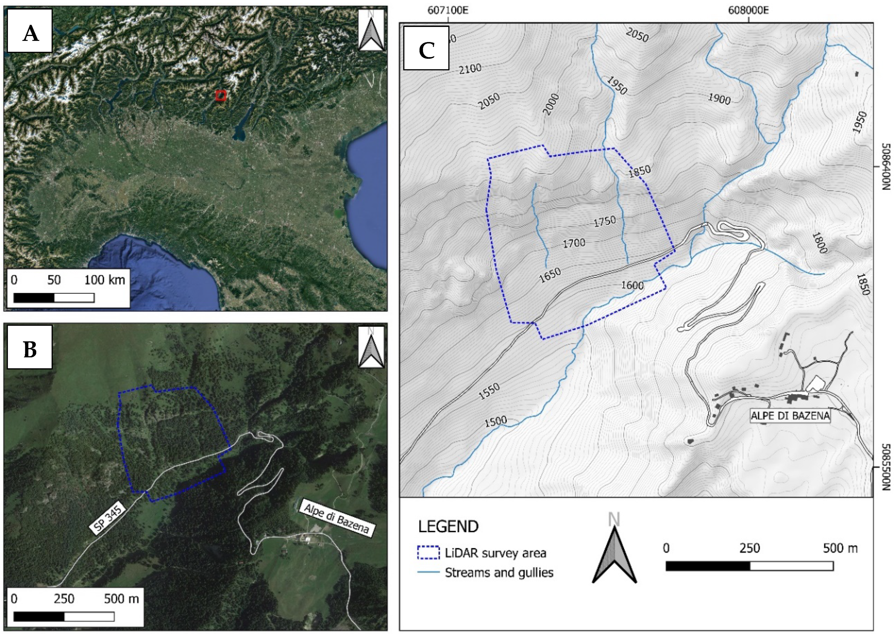
The algorithm was tested in a known study area where rockfall is quite common. The output data were compared with the results obtained employing the conventional stereoplot approach, iterated enough times, and considering a suitable set of orientations for the rockface. The results show that the algorithm works as intended and produces more reliable data since it considers the local orientation of the rock face instead of deterministic reference values.

2. Materials and Methods

The authors developed an automatic procedure for performing Markland’s tests for PS, WS, and TP (at this stage, only flexural toppling is considered), based on slope and aspect data of the DTM of the studied area, combined with on-site geomechanical survey data. In the following paragraph, the input data, the algorithm’s functioning, and the output are described in detail.

2.1. Input Data

As stated before, the required input data are a DTM of the rock mass and data describing the joint sets surveyed in that rock mass.

Once the DTM has been imported into QGIS, one must select the area that includes the rock faces and crop it. It can be easily performed in QGIS by employing the Clip Raster by mask layer tool located in the Raster > Extraction menu. This operation requires, though, to have already defined a vectorial shapefile layer containing the spatial distribution of the rock faces, which act as a mask to extract the relevant part of the analyzed DTM. This information can be obtained in a plethora of ways: the easiest approach consists of mapping rockfaces traditionally on the field and then digitalizing them. Alternatively, the mask polygon can be drawn from orthophotos or satellite imagery. There is also the possibility of extracting the position of rockfaces from the DTM, for example, employing one among the different methods suggested in the literature [15,16,23,24]. Once the mask layer is defined, and the required portion of DTM is cut out, the information on slope and aspect needs to be extracted. This operation is performed employing the slope and aspect tools of QGIS, located in the Raster > Analysis menu. For the purpose of the algorithm, it is essential that slope and aspect raster grids have the same size and spatial resolution. Each cell of the slope matrix contains the rockface local inclination, which is the angle describing how inclined the surface of the pixel is (i.e., the dip of the pixel). Similarly, each cell of the aspect matrix contains the azimuth of the dip, namely the angle between the north and the direction towards which the pixel is inclined (i.e., the dip direction of the pixel). By combining slope and aspect data, the orientation of the rockface is defined in each location of the considered area. Therefore, it can be assumed as the orientation of the front in Markland’s tests. Once the slope and aspect raster have been extracted, they need to be saved as GeoTIFF files so that the data regarding georeferencing stored in their metadata can be later employed to define the output files. The GeoTIFF format was chosen because it is the most common type of raster file used when dealing with geographically significant information. It is important to stress that the source of the DTM is not relevant. Since the algorithm works starting from the slope and aspect raster grids extracted from the DTM, the only important feature is that the rockface is modeled by the DTM properly and at a reasonable resolution.

Regarding the joint sets, the required input data are simply records of three angular values for each set recognized in the rock mass, describing its dip, dip direction, and friction angle. This information can be derived either from traditional geomechanical surveys carried out in the study area or from non-contact methods. In any case, it is essential to stress the relevance of a field survey to have a sound knowledge of the discontinuities in terms of the number of joint sets and their mean orientation. Moreover, it is fundamental to identify if there is a need to divide the rock face into homogeneous portions with regard to the joint sets. In other words, it is required to check if the dip/dip directions values found for each set are significant in the entire analyzed surface or if there are some portions where these values change, or if new joint sets exist. Therefore, the reliability of the process is based on the consistency between the modeled area, the input data, and the actual rock mass structure. Once the joint sets have been recognized, a reference value for their dip, dip direction, and friction angle is stored in a text file: the information has to be reported in this exact sequence for the algorithm to read it correctly.

2.2. Tool Functioning

The code was developed in the Matlab environment to take advantage of that language’s great flexibility and the opportunity to manage GeoTIFF files and their metadata. In particular, the function geotiffinfo returns a structure whose fields contain image properties and cartographic information. The function geotiffwrite allows one to create a GeoTIFF file based on an image and the associated cartographic information. This means that one can import a GeoTIFF file, process the image while keeping its cartographic information, create a new image representing the result of the performed operations, and then build another GeoTIFF file associated with the original cartographic information. Therefore, the input and the output file can be directly managed in the same reference system, avoiding the need to define anew every time the georeferencing of the output data files.

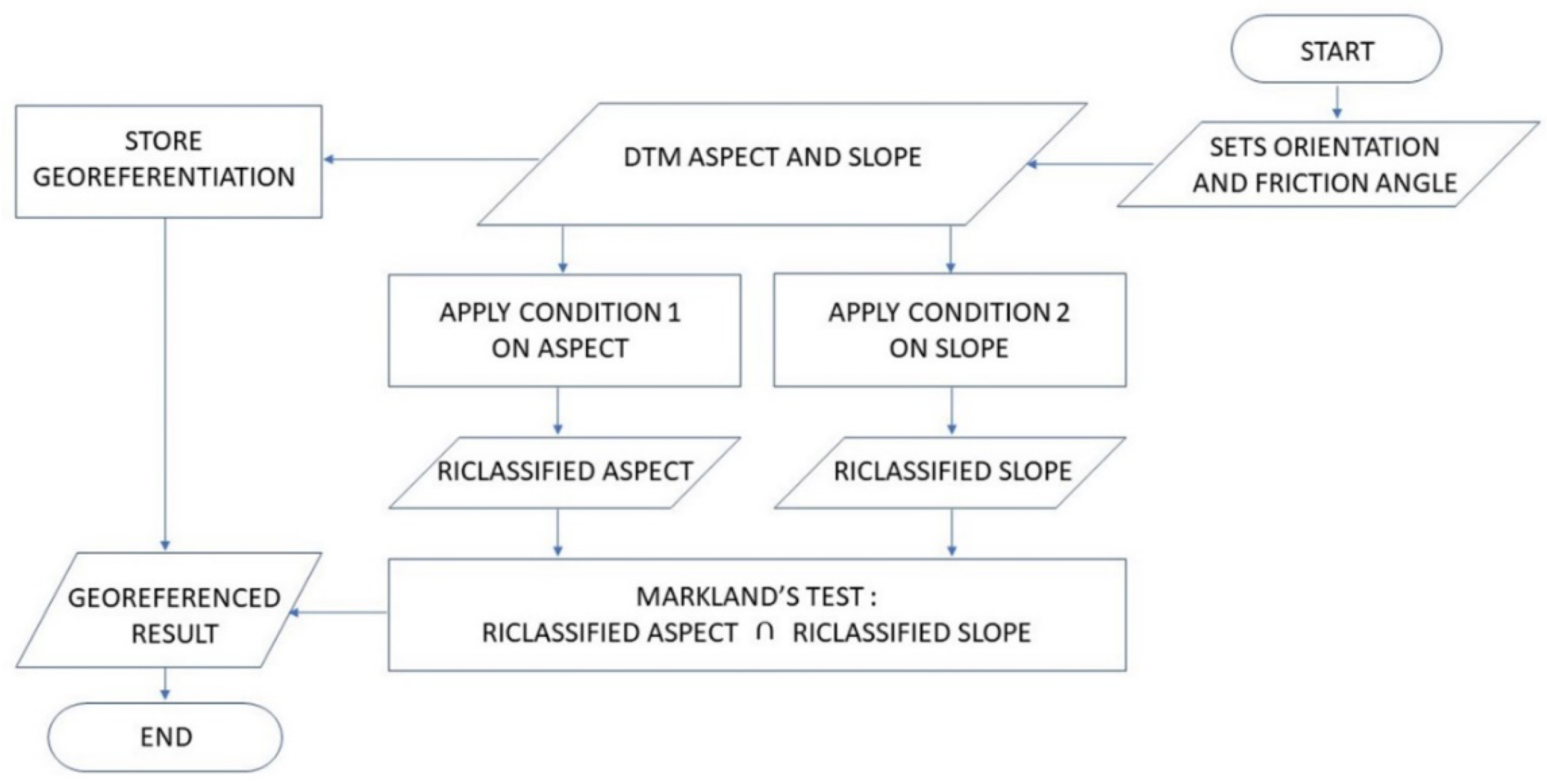
The conceptual workflow of the functioning is shown in Figure 1. As described in detail in the previous section, input data consist of three elements: two GeoTIFF files containing aspect and slope information of the considered rockface and a text file containing orientation and friction angle of all the n discontinuity sets. The code performs Markland’s test for PS, WS, and TP; the output file of each of these three tests consists of a GeoTIFF file whose image is basically a matrix of results and whose metadata are the same as those of the input GeoTIFF files. In detail, the images have the same size, corresponding to the considered area of the DTM on the horizontal projective plane, and the same spatial resolution, equal to that of the input GeoTIFF files. Then the three resulting files are summed, and the final output is produced. It contains a matrix of values; the higher the value of a matric cell, the higher the number of possible kinematics among all the investigated ones the cell is geometrically allowed to produce. Namely, it represents a map of potential source areas in which each cell of the DTM area contains a rate of the kinematic predisposition to the tested phenomena. Lastly, the algorithm generates a simplified copy of this last output file, containing only the information concerning the position of the cells where the kinematic test was positive at least once.

The detailed workflow describing the implementation of Markland’s tests in the developed tool is shown in Figure 2. Once assigned the input files, two conditions must be verified simultaneously to result in a positive response (i.e., to pass Markland’s test positively). These conditions are different based on the considered phenomenon [2,3]. In particular, for PS and TP, the conditions concern a single discontinuity set at a time, while for WS, they consider the intersection of two sets forming a wedge. Therefore, each set is tested for PS and TP; each combination of two sets is tested for WS. The process is fully automatic and produces a certain number of reclassified matrices, namely matrices whose size and spatial resolution are the same as the original ones and whose content is the response to the test evaluated in each cell.

Considering PS, the first discontinuity set is considered for testing its capability of producing PS with respect to the local front of the rock face. Condition 1 is applied to each aspect matrix cell: if the condition is verified in a cell, a logical true (one) is assigned to the corresponding cell of the reclassified aspect matrix; otherwise, a logical false (zero) is attributed. Then Condition 2 is applied to each cell of the slope matrix, and the same procedure is performed by filling the reclassified slope matrix. After that, the code performs Markland’s test for PS by checking cell by cell the intersection (logical AND) of reclassified aspect and reclassified slope; the result, which is still a logical true or false, is assigned to the corresponding cell of the result matrix. The logical values of the resulting matrix are then converted into double values, which are zeros or ones, producing a matrix called PS1. The procedure is repeated for each of the n discontinuity sets, producing PS2, …, PSn. In the end, the matrices PS are summed element by element, giving another matrix, called PSsum, in which the values of the cells are integers that can vary between 0 and n, where 0 means that the PS test is negative for all the sets. Therefore, no planar sliding phenomena are kinematically feasible in that cell. Values greater than 0 mean that one or more of the discontinuity sets give a positive response to the test.

The test for TP follows the same procedure, producing matrices TP1,…, TPn and TPsum.

The test for WS follows a very similar procedure, with the only difference being that it considers the pairs of discontinuity sets that intersect and produce a wedge. Therefore, for n sets, there will be m pairs, where:

m = n! / (2! (n − 2)!)

(1)

Test for WS will be performed m times and produce matrices WS1,…, WSm and WSsum.

Finally, matrix S, equivalent to the sum of the effects of each of the three main kinematisms, is calculated:

S = PS_sum + TP_sum + WS_sum

(2)

By reclassifying the S matrix by setting every cell with a value above 0 as a 1, the last output matrix is defined; it simply describes the location of all the cells where the kinematic analysis allows for instabilities. Therefore, it is a handy tool for defining source areas in numerical simulations, for example.

2.3. Output Data

All the created matrices are associated with the original cartographic information and saved as GeoTIFF image files using the geotiffwrite function of Matlab. This means that by simply importing the freshly created GeoTIFF files into QGIS, they will automatically be fixed in the same position as the original slope and aspect files required as input. Simply modifying the symbology of these newly imported raster layers allows for quick and straightforward visualization of the results. Moreover, if need be, in QGis is very easy to export the output files in a different format than GeoTIFF or even convert the output data from a raster grid to vectorial: for example, using the r.to.vect tool in the GrassGis repository, which provides in input a shapefile format vector (points, lines or polygons).

3. Case Study

3.1. Study Area and Input Data

The case study chosen to show how the algorithm performs is in Lombardy Region (Northern Italy), in the municipality of Breno (Brescia province). The site is located just south of a place known as Alpe di Bazena, along a key provincial road (SP 345) that connects the towns of the area to a regionally important mountain pass by the name of Crocedomini Pass. Along this section of SP 345, the northern slope is characterized by the presence of steep talus deposits, more or less vegetated, culminating in a series of rock faces near the ridge line, with a height up to more than 150 m. These rock faces produced a significant number of rockfall events over the years, most of which were stopped by vegetation before interacting with the existing protection works located along the SP 345 road. Figure 3 summarizes this information, while the photo in Figure 4 gives an idea of the study area.

The rocky slopes of the area have been carved into the limestone of the bedrock through a combined effort of gravitational processes, surface runoff, and avalanches. The result is a quite complex morphology, with very few clear and regular surfaces cut by deep incisions and a well-developed talus deposit stretching down towards the road and beyond. In general, the slope is nevertheless highly inclined, with an average inclination of 38°. The rocky ridge at the top is, of course, the steepest portion: in some areas, the slope is almost vertical (88°). The slope average exposition (or aspect) is towards SSE.

A field survey allowed mapping of the surface of the rock faces; through a series of traditional contact surveys carried out on the accessible outcrops at the base of the rock mass, raw orientation data were obtained for the entire rock face. By processing and analyzing the raw data, four joint sets (K1 to K4) were recognized: three of them are joint sets, while K2 describes the bedding of the rock; this information is summarized in

Table 1. The four joint sets recognized in the rock mass of the study area.

Set	Dip	Dip Direction	Joint Type
K1	58	253	Joint
K2	73	047	Bedding
K3	45	360	Joint
K4	83	280	Joint

. The use of reference values to describe the discontinuities in the rock mass defines a deterministic approach. The rock mass generally appears quite fractured and weathered superficially, showing a blocky appearance. Moreover, it can be stated that there are no significant local variations in the geological, structural, or geometrical features of the rock mass. Therefore, the entire rock face has been considered a homogeneous domain.

Since no tests to define the friction angle of these joint sets have been carried out, the standard value of 30° was assumed. This value has been used extensively in the literature when dealing with rocks of unknown mechanical properties [3,25,26].

By using a DTM derived from a LiDAR survey carried out in the area, the input raster data for the algorithm were extracted. The DTM has a spatial resolution of 0.5 × 0.5 m, and the elevation has a resolution of 0.2 m. The spatial resolution of the original DTM was preserved for all the other raster files in input and output. The slope and aspect of the study area obtained following the procedure described in Section 2.1 are visible in Figure 5 and Figure 6.

3.2. Algorithm Results and Crosschecking

Once the input data were produced, the algorithm elaborated them and gave the output GeoTIFF files. In order to check and validate the results, a series of traditional Markland’s tests were performed, employing the original stereoplot approach.

With this in mind and considering the complex morphology of the rock faces of the study area, it is evident the need to define a sufficiently wide set of significant dip/dip direction pairs to describe the rock face surface locally. For this purpose, the authors chose to focus on the information regarding slope angle and aspect limited to the rock faces only (Figure 7). The idea was to identify dip/dip direction pairs (i.e., slope/aspect) that could describe in the best way the complex morphology of the rock faces mapped in the case study area.

Regarding slope angle, which defines the dip of the topographic surface, it should be taken into account the fact that the average value for the rock faces is equal to 62°: as it can be seen in Figure 7 lower half, the rock faces are characterized by highly steep portions (>70°) bordering less steep surfaces (<60°). Given that the dip of the reference surface directly influences the area on the stereoplot describing dip/dip direction combinations where movement is geometrically possible, it is reasonable to state that the average value does not cover all the possible range of slope values, given that, as stated in the previous paragraph, the maximum value of the slope angle is 88°. It is, therefore, reasonable to employ this maximum value rather than an average one.

Regarding the aspect, which defines the dip direction of the topographic surface, the definition of reference values requires an analysis of the actual distribution of aspect angles: an initial overview is given in Figure 7, upper half, where eight 45° wide classes are used to map the aspect as calculated from the DTM. It can be seen that the colors used in the figure tend to define three main aspect groups: the first, second, and third classes, which describe the portions of the rock faces oriented towards NE to E (shades of blue); the fourth class and part of the fifth, which describe the portions of the rock faces oriented towards SSE to SSW (green and yellow); the other three classes, which describe the portions of the rock faces oriented towards W to NW (shades of orange). These three groups show that the complex morphology of the rocky portion of the studied slope can be described in an extremely simplified way using three rock face orientations: towards ENE for the first group, towards SSE for the second, and towards W for the third. Almost no position on the rock faces appears to be oriented towards N: this is reasonable, given that the slope is on the southern side of a ridge. Figure 8 shows this simplified classification of the rock faces aspect. By relying on this information, it is possible to define three pairs of dip/dip direction values describing the orientation of the simplified rock faces to be used in the traditional Markland’s stereoplot tests (

Table 2. Pairs of dip and dip direction values used to simplify the complex morphology of the rock faces into three faces (F) only.

Class	Dip	Dip Direction
F1	88	65
F2	88	165
F3	88	275

). The friction angle reference value is the same input in the algorithm, namely 30°.

In order to check if the results produced by the algorithm are correct and therefore acceptable, each of the output sum files, conveying the global result for every one of the three types of movement (PS, WS, and TP), were compared with the respective kinematic test performed on stereoplots for each of the three reference rock faces (F1 to F3).

Figure 9, Figure 10 and Figure 11 show the aforementioned output files and the equivalent stereoplot kinematic tests. The global sum file S defined accordingly to Equation (2), which summarizes all the tests performed by the algorithm into one easy-to-read image, appropriately colored, is presented in Figure 12. Considering how it is defined, this S image gives a quick view of the sectors of the rock faces of the study area where the movement of blocks is more favored by the discontinuity assets, and as such, this image shows an index of likeliness of movement. Lastly, for a complete overview of the output files, the reclassified version of image S is also shown in Figure 12: in this particular case, the output file was converted to a vectorial shapefile by using the r.to.vect tool of the GrassGis repository, available within QGis. This last output file is intended to be used as the definition layer of rockfall source areas, as it maps all those cells of the DTM where at least one of the three types of movement has been proven possible by the kinematic tests.

4. Discussion

An analysis of the output files of the algorithm with respect to the corresponding results of the manual procedure is reported hereinafter.

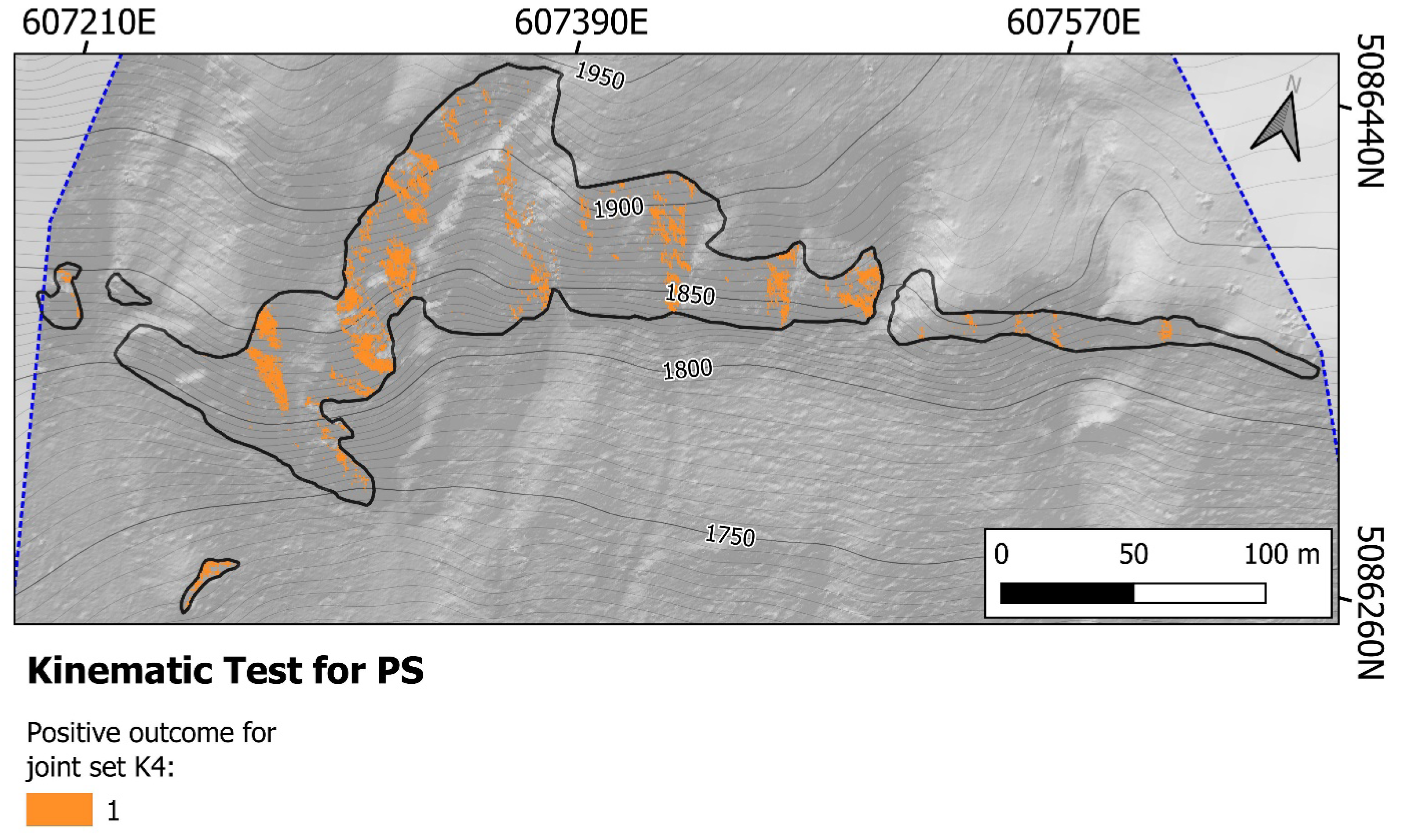
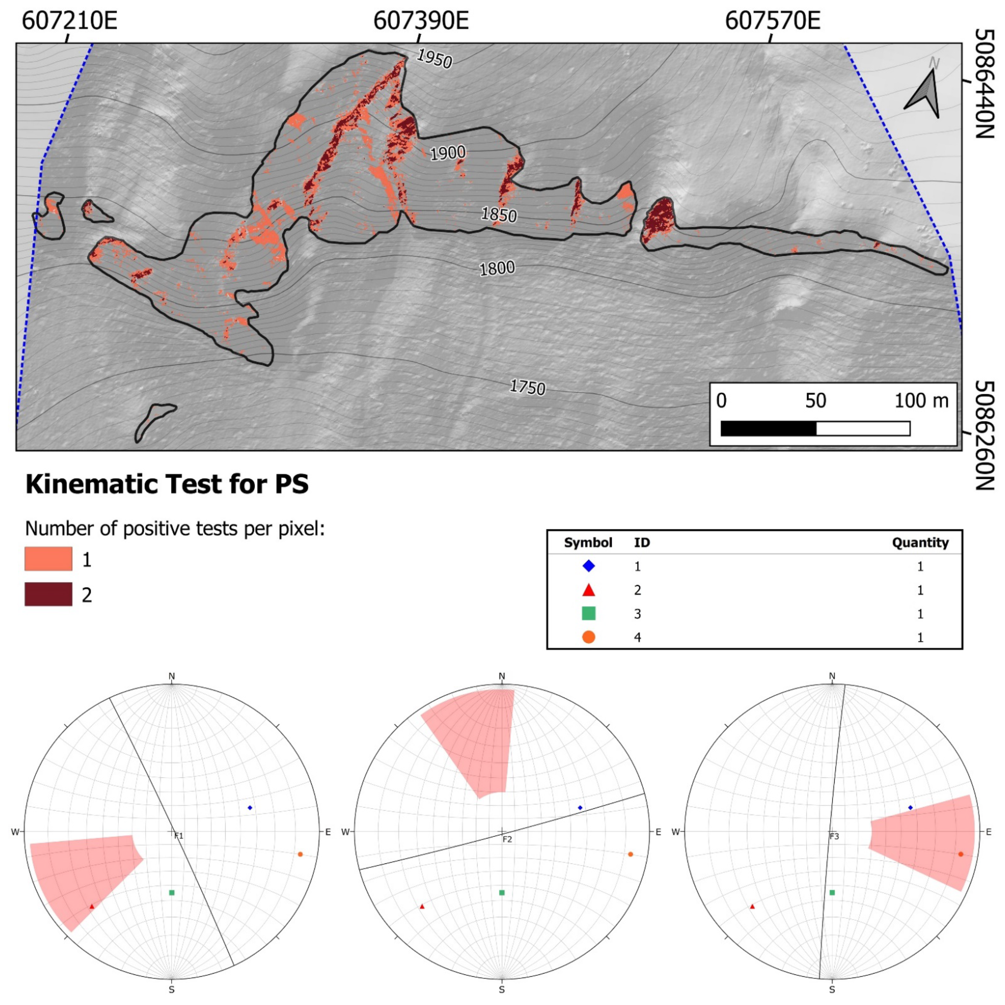
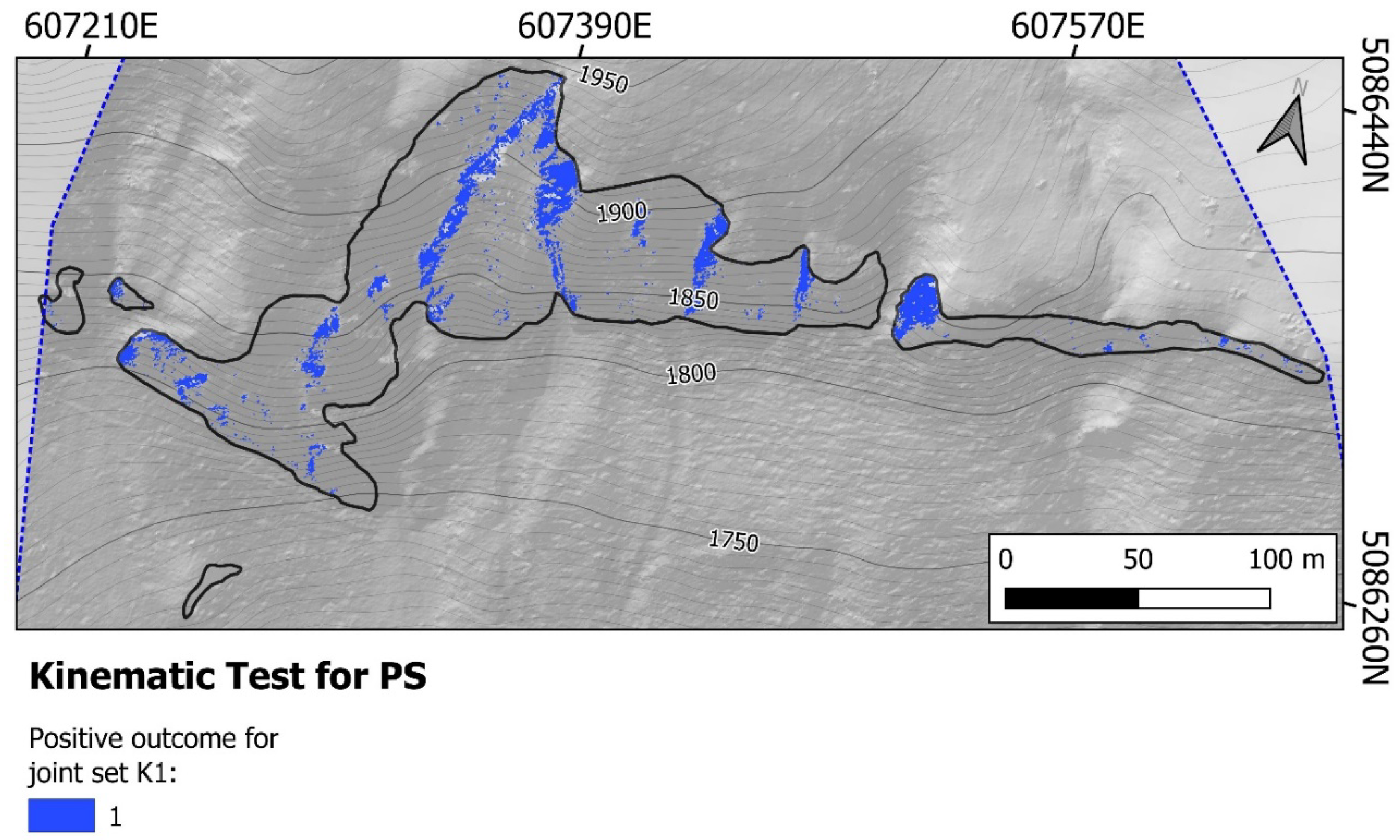
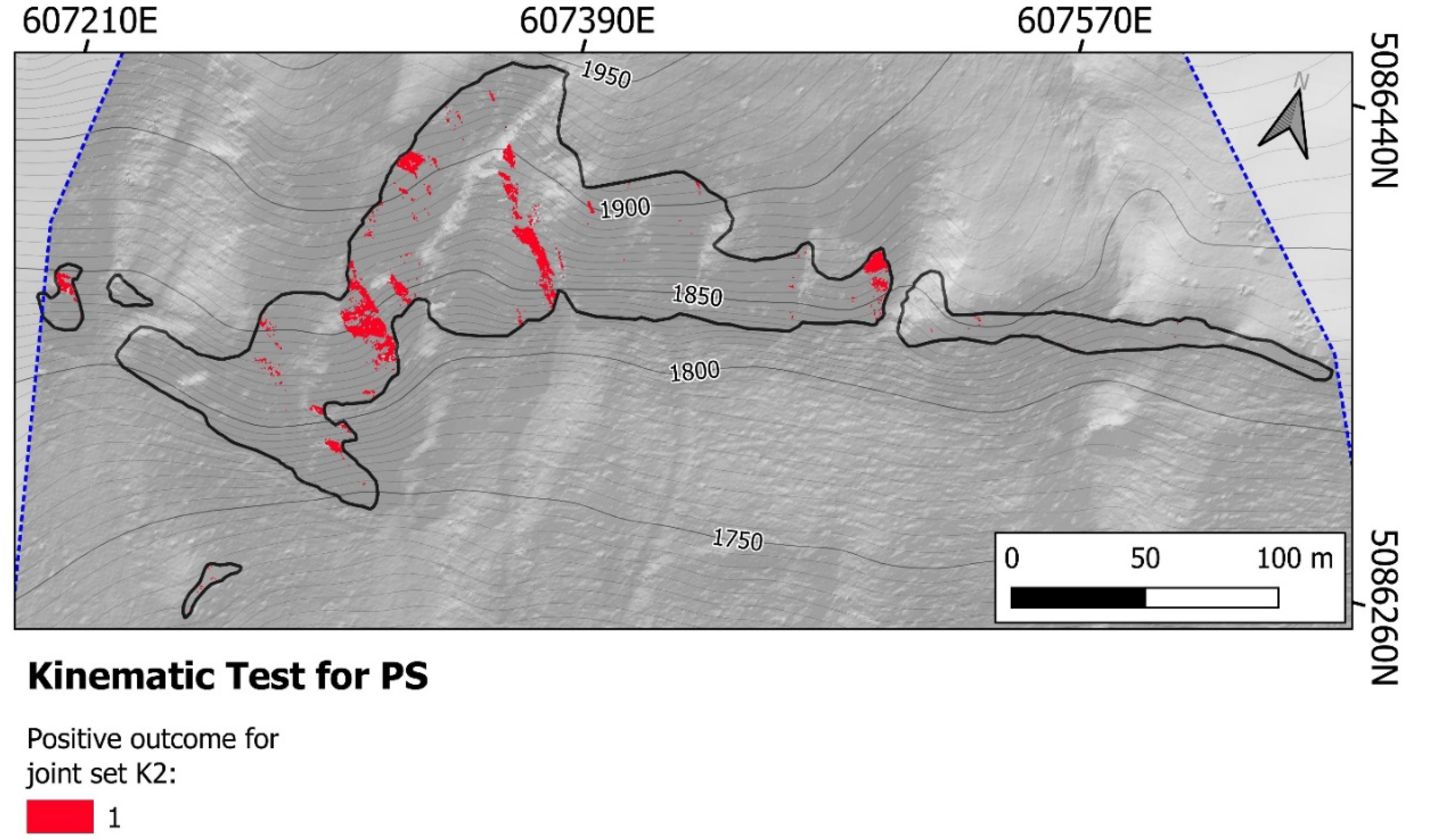
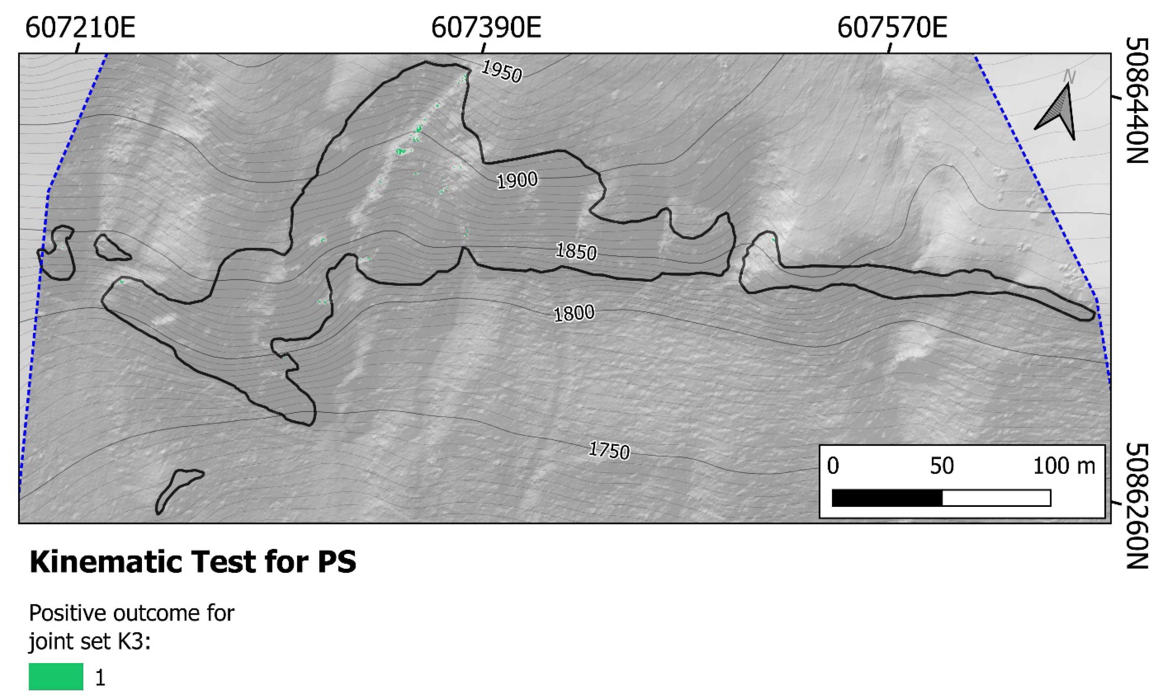
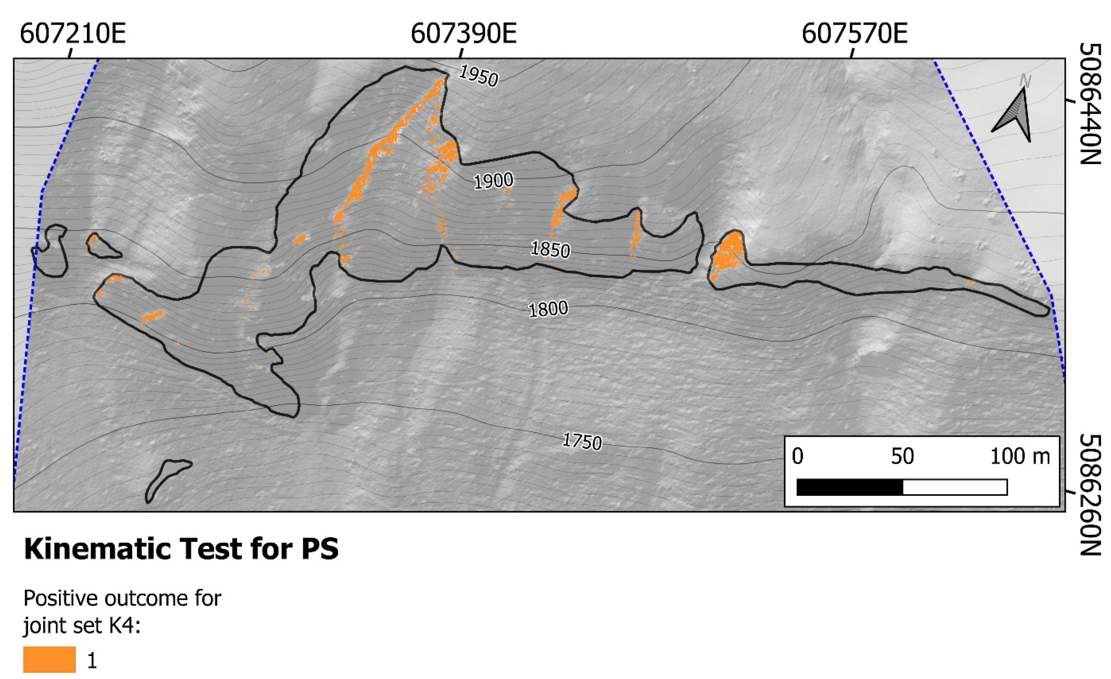
The first of the output sum files of the algorithm is PS_sum, which features the results of Markland’s test for all the possible predisposing assets for planar sliding. As shown in Figure 9 upper half, only two classes (described as shades of red) are present. It can also be seen that the portions of the rocky slope where two joint sets yielded positive results for the kinematic analysis are quite distinct from the remaining portions where only one joint set gives positive results. In order to evaluate which set is responsible for the information conveyed by the PSsum matrix, it is necessary to visualize one by one the partial output files produced by the algorithm for each joint set: this operation is reasonably short, given the fact that these partial output files are named after the set and contain in their pixels only 0 or 1, if the kinematic test is negative or positive, respectively. In this particular case, all sets are actually active, but the positions where they tested positive appear to overlap only in localized areas. 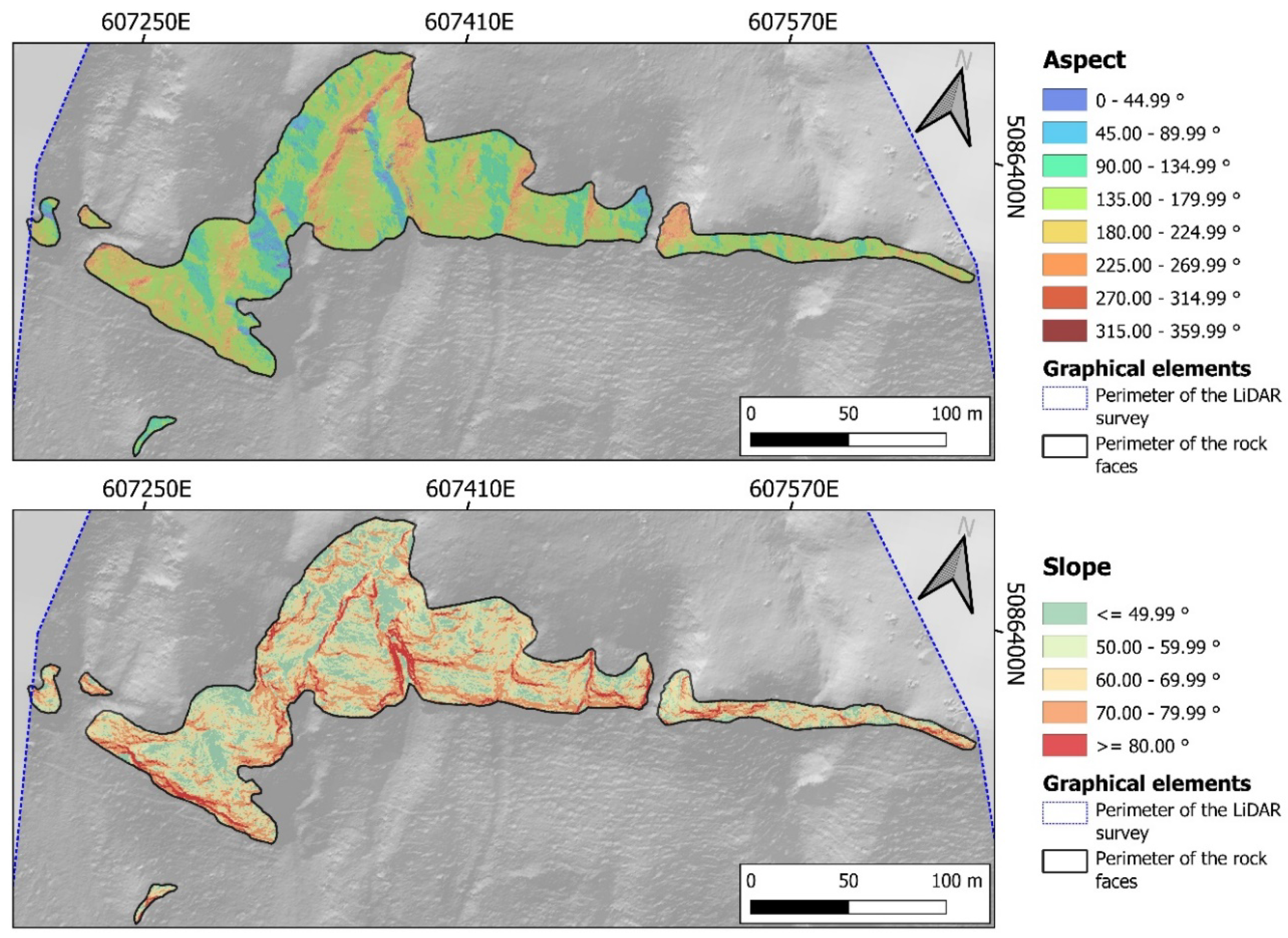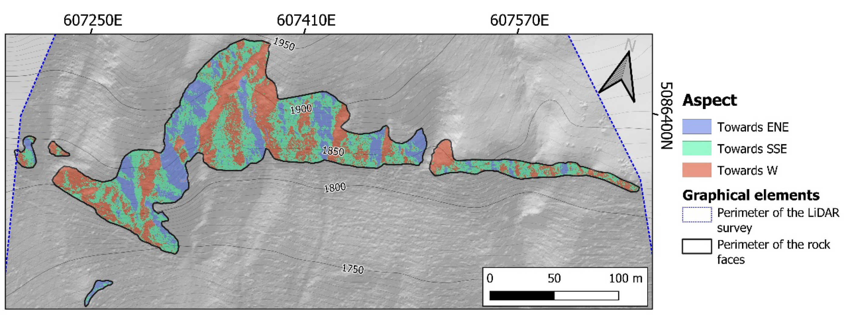If the simplified aspect map of the rock faces (Figure 8) is taken into account, we can see how the locations where only one set is active at a time are aligned along the portions of the rock faces exposed toward E – ESE. On the other hand, the parts where two joint sets are active lay on sectors of the rock faces exposed towards W: these portions are usually located along the eastern slope of the incisions that divide the rocky slope into many rock faces. Therefore, it should be expected that of the three stereoplot depicting the traditional Markland’s tests, only the two featuring the F1 and F3 configuration of the simplified rock face produce positive outcomes. In Figure 9 lower half, we can see that in the case of the F1 configuration, joint set K2 gives positive results, while in the F2 configuration, no joint sets satisfy the required conditions to pass the kinematic test. Lastly, the F3 configuration establishes that the W-ward-oriented surfaces can produce positive outcomes for K2. It should be noted that surfaces oriented slightly more towards WSW than F3 could interact positively also with K1. Therefore, the three traditional stereoplot tests prove the algorithm PS_sum output matrix is correct. For convenience, the partial output files for each joint set are shown in Appendix A (Figure A1, Figure A2, Figure A3 and Figure A4).

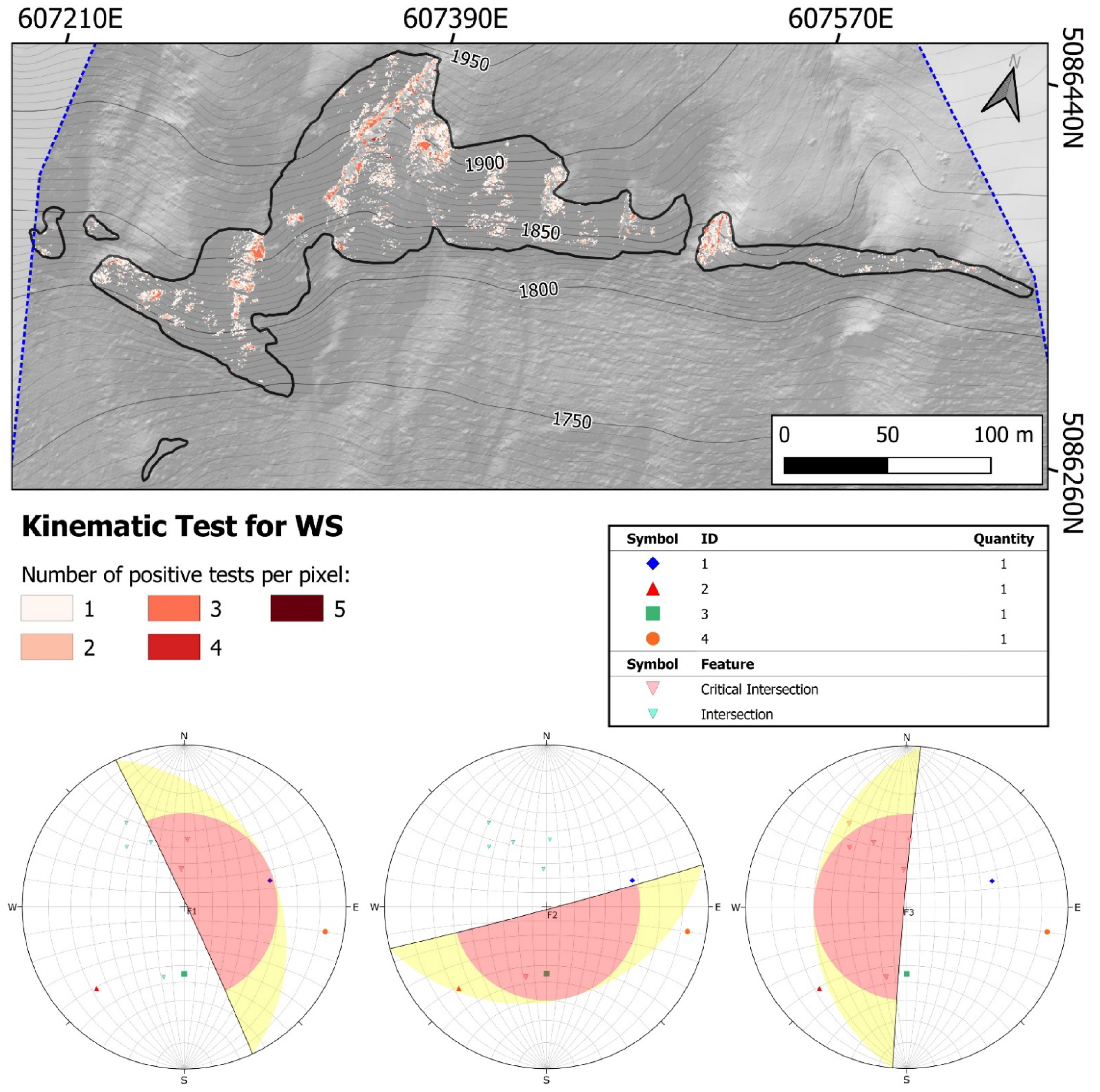
The second output sum file is WS_sum, which features the results of Markland’s test for all the possible predisposing assets for wedge sliding. The first half of Figure 10 shows that there is a wide spread of this type of movement, and up to five different intersections between sets can produce it, as shown by the different shades of red among the six possible calculated following Equation (1). Almost all the sectors of the rock faces, where the high level of activity of these five intersections is located, lay along the eastern side of incisions, carved into the bedrock by surface runoff or avalanches. It is possible to notice how the distribution on the rocky slope of the pixels that tested positive more than once follows approximately the distribution of the surfaces exposed westwards in the simplified aspect map (Figure 8). The pixels that test positive only once appear instead quite dispersed, mostly over the surfaces exposed towards SSE but also on those oriented eastwards. It is reasonable to expect that the stereoplot kinematic test showing the F3 configuration would produce positive results for almost all the intersections; for the other two configurations (F1 and F2), at least one intersection should give positive results when performing the traditional stereoplot Markland’s tests. In the lower half of Figure 10, we can observe that this reasoning is verified: In the F1 configuration, two intersections test positive, and it can be seen that for eastward exposed surfaces, there is always at least one intersection satisfying the required conditions; for configuration F2 similar conclusions can be drawn. In configuration F3, one can observe up to five intersections testing positive, while a sixth one is almost inside the red polygon where the positive results lay. 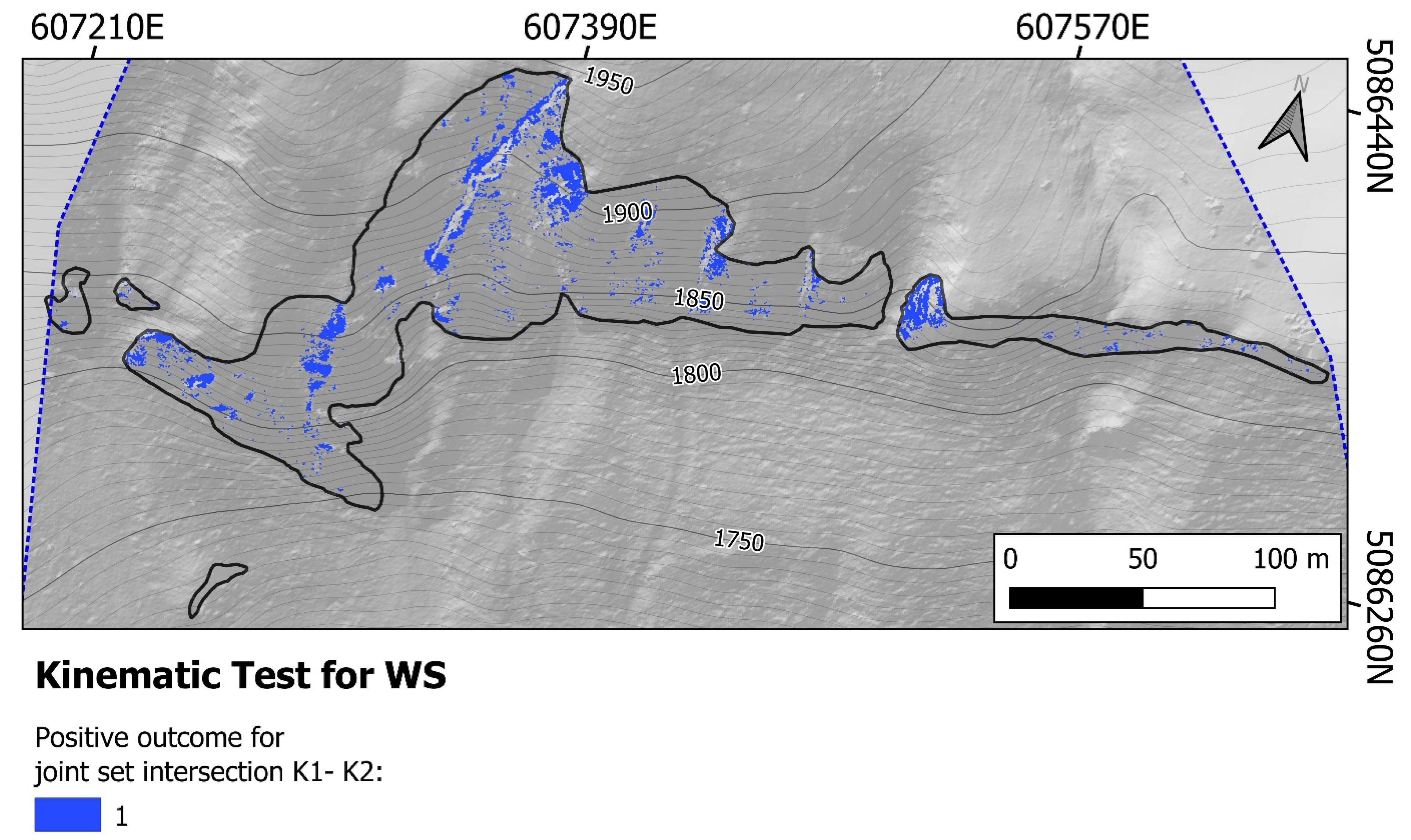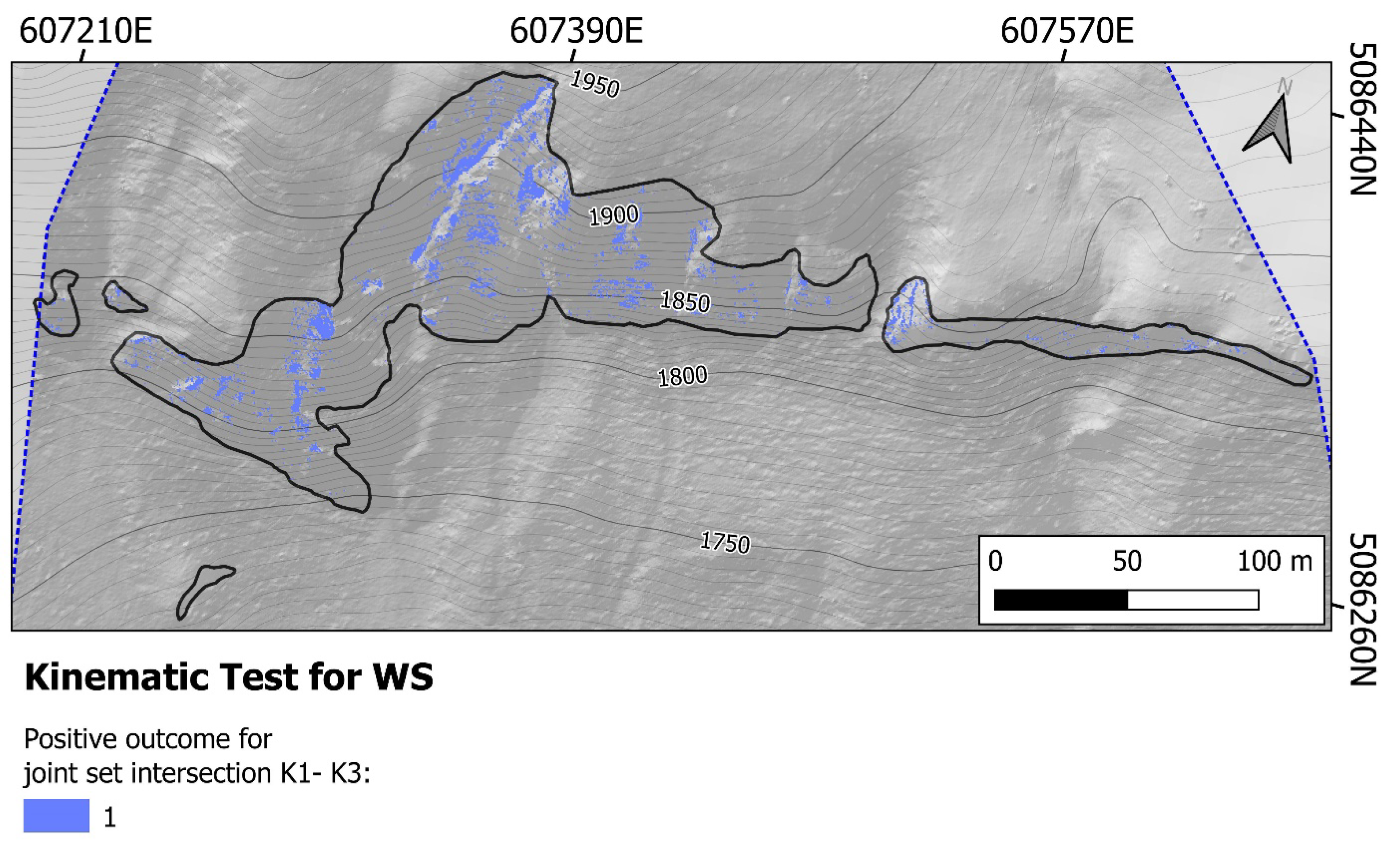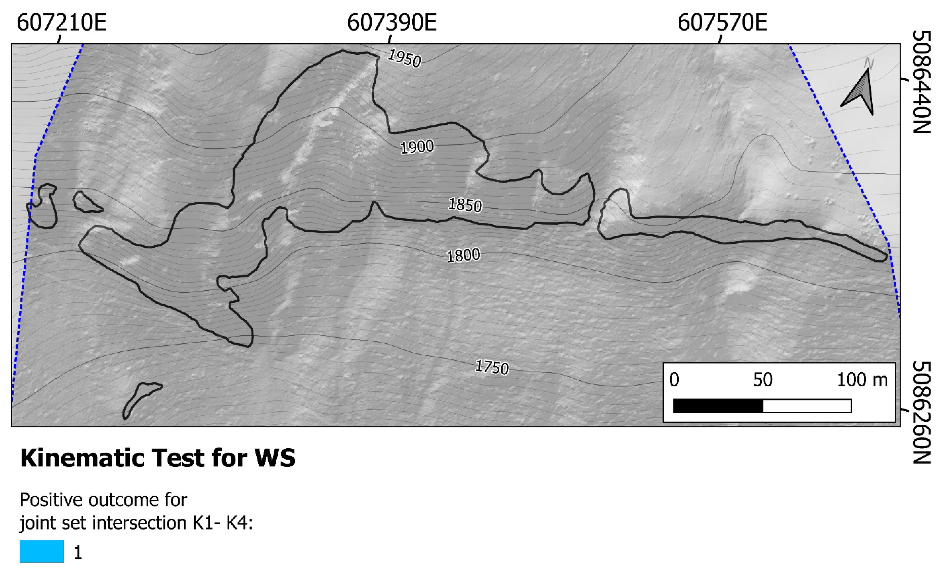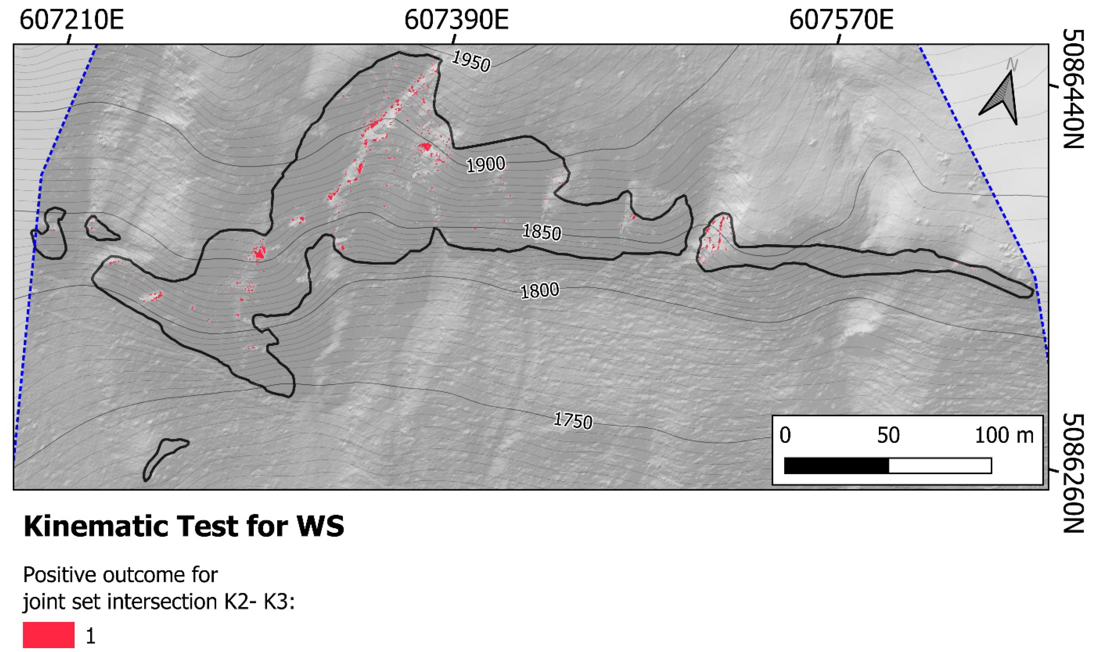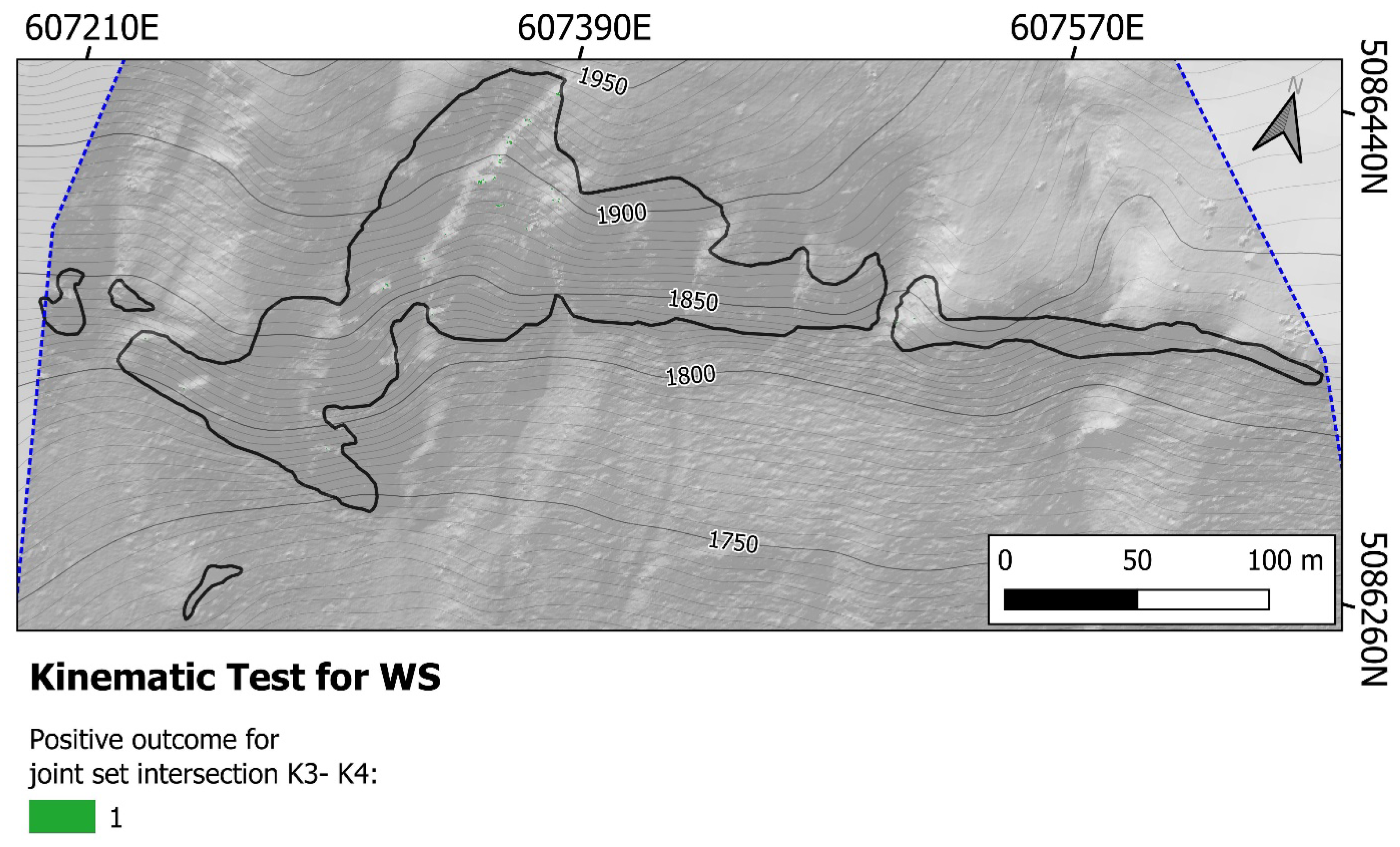Therefore, the three traditional stereoplot tests prove the algorithm WS_sum output matrix is correct. Once again, if one needs to verify which intersections are actually active at a given position, then the partial output files should be visualized: these files are named by the algorithm following the names associated with the two intersecting joint sets. As for the previous case, the WS partial output files can be found in Appendix A, in Figure A5, Figure A6, Figure A7, Figure A8, Figure A9 and Figure A10.

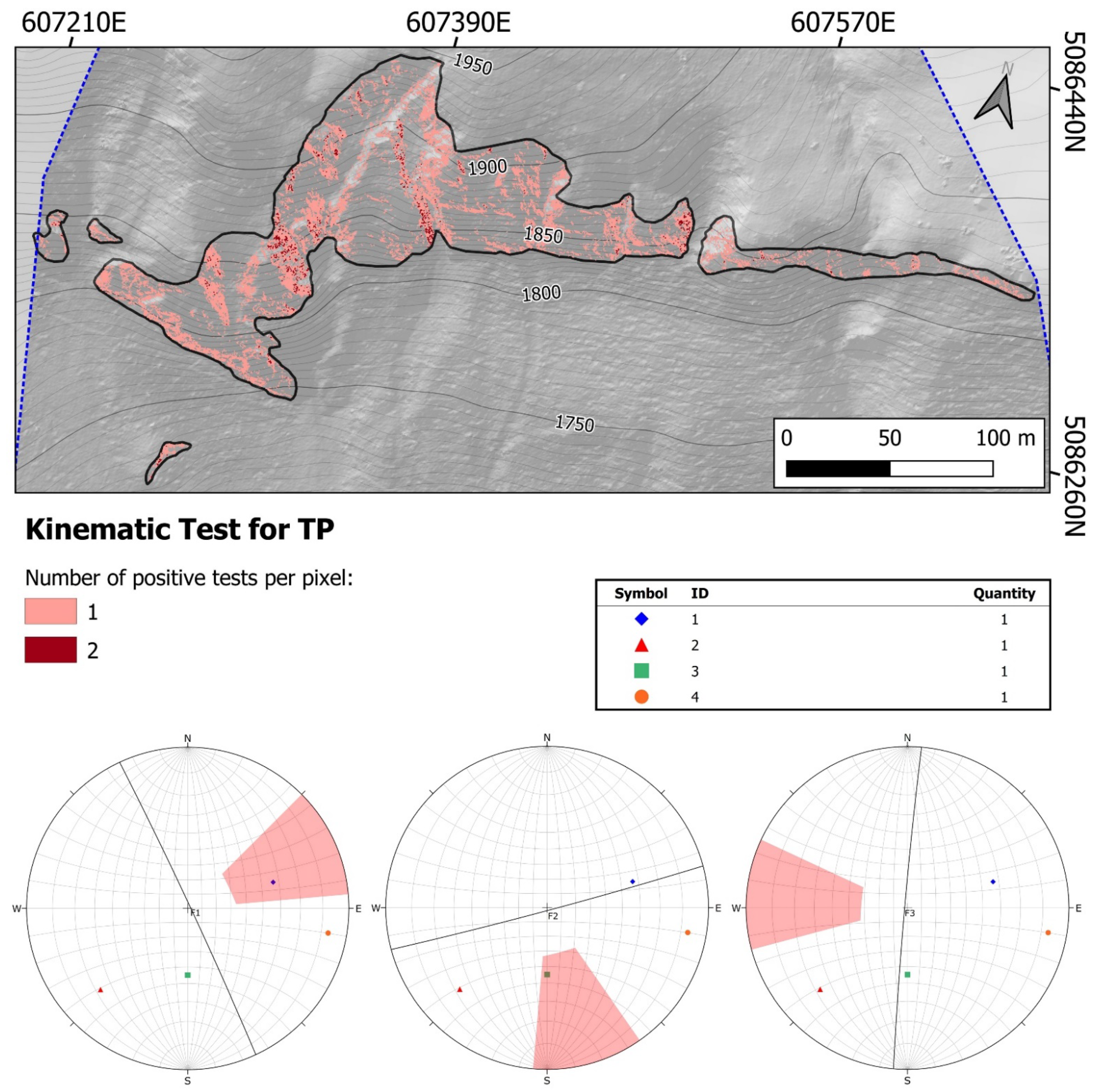
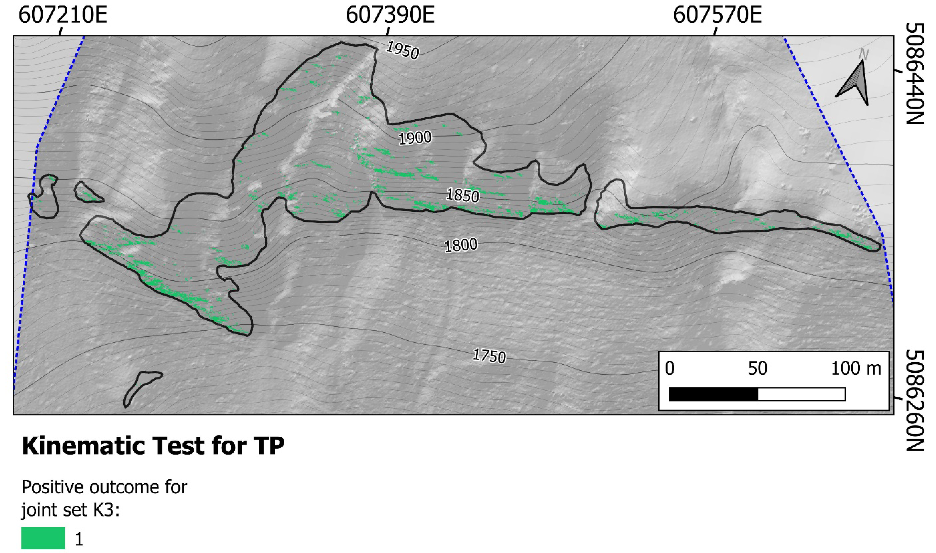
The third output sum file is TP_sum, which features the results of Markland’s test for all the possible predisposing assets for flexural toppling. An observer can gather from the first half of Figure 11 that TP is widespread on the rock faces of the study area, even more than WS. Moreover, if the simplified aspect map (Figure 8) is taken into account, no evident correspondence to one of the three orientation classes can be noted for the positions where only one joint set at a time tests positive (lighter shade of red). It can be observed, though, that the eastward exposed surfaces of the rock faces fit well with the distribution of the locations where more than one joint set at a time tests positive (darker shade of red). These considerations allow foreseeing that in all three stereoplots depicting simplified rock face configurations F1 to F3, at least one set should yield a positive outcome, while only on F1 two joint sets should. 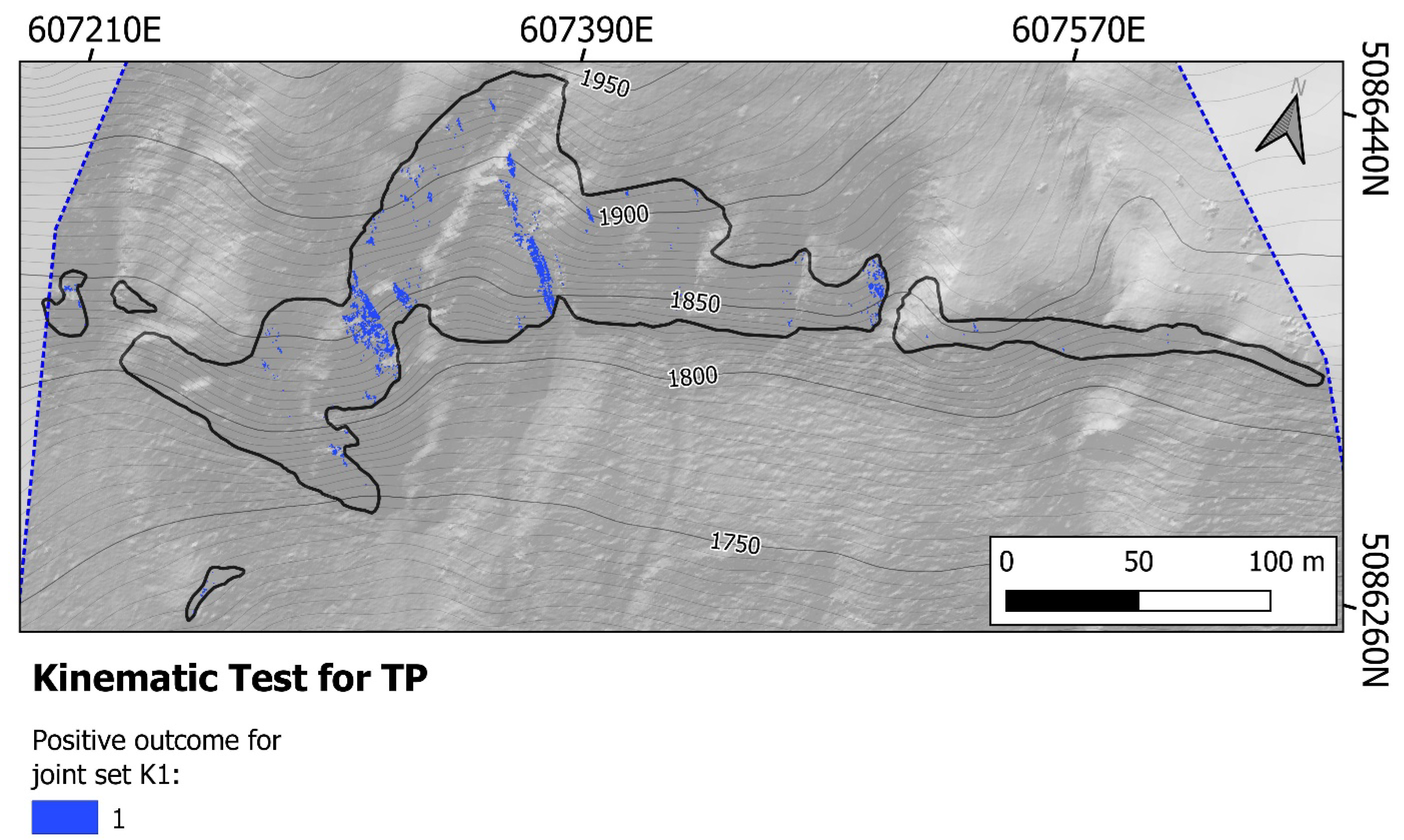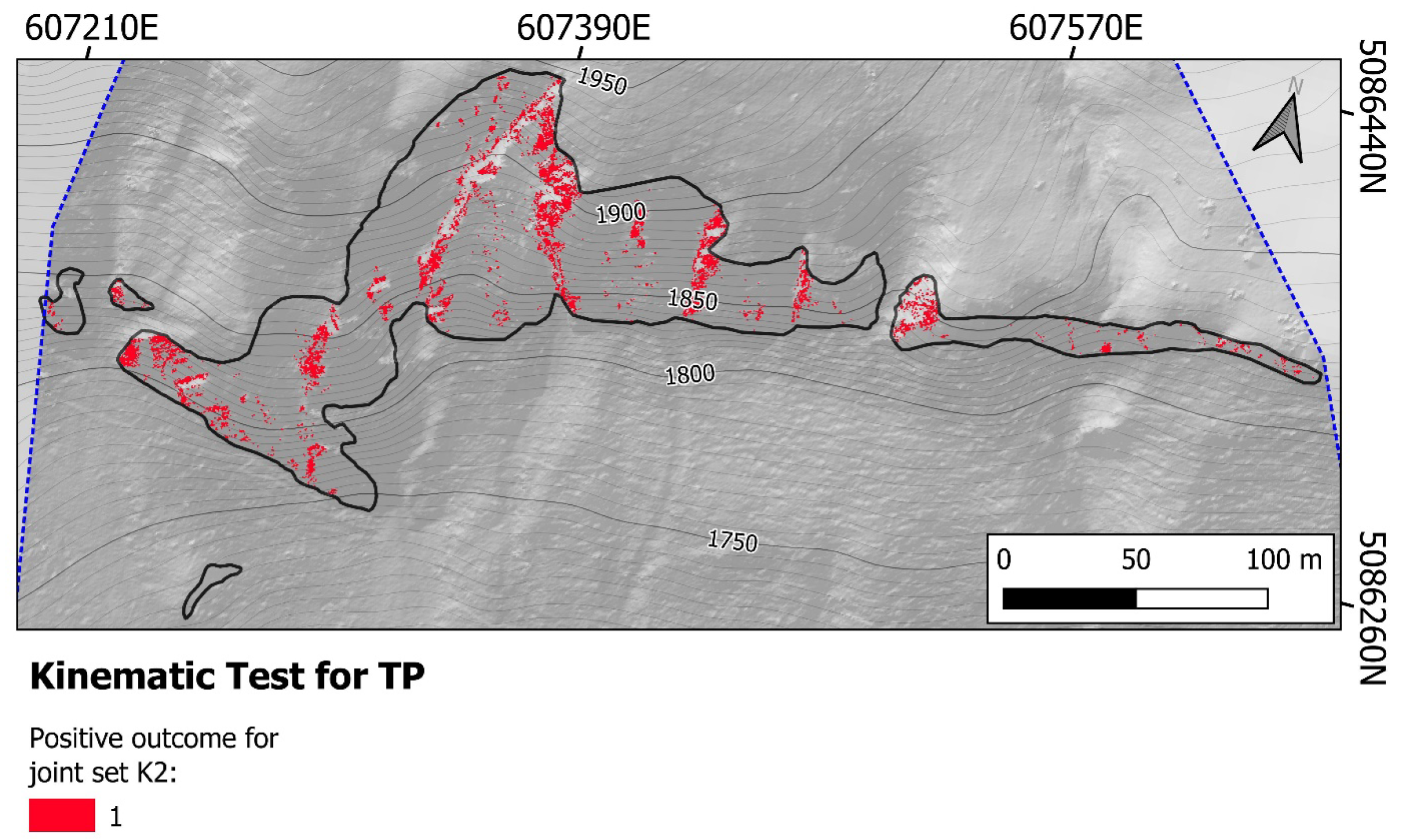In fact, the second half of Figure 11 conveys information not far from what was foreseen. For F1, it can be seen that only joint set K1 satisfies the required conditions, but for surfaces exposed more towards E or ESE, joint set K4 would also give positive results; for F2, joint set K3 satisfies the requirements in each stereoplot; lastly, for F3, there are no active joint sets, but in the case of SW oriented surfaces, joint set K2 would test positive. It should be noted that, by analyzing the partial output files, it was found that all joint sets produce positive results. This is in line with what the traditional stereoplot tests show, given that for surfaces either equivalent to F1 to F3 or not too different, all four joint sets yield positive outcomes at least once. Therefore, the crosscheck performed employing traditional stereoplots confirms the output of the algorithm. As for both the PS and WS cases, also for this one, the partial output files for each joint set can be found in Appendix A (Figure A11, Figure A12, Figure A13 and Figure A14).

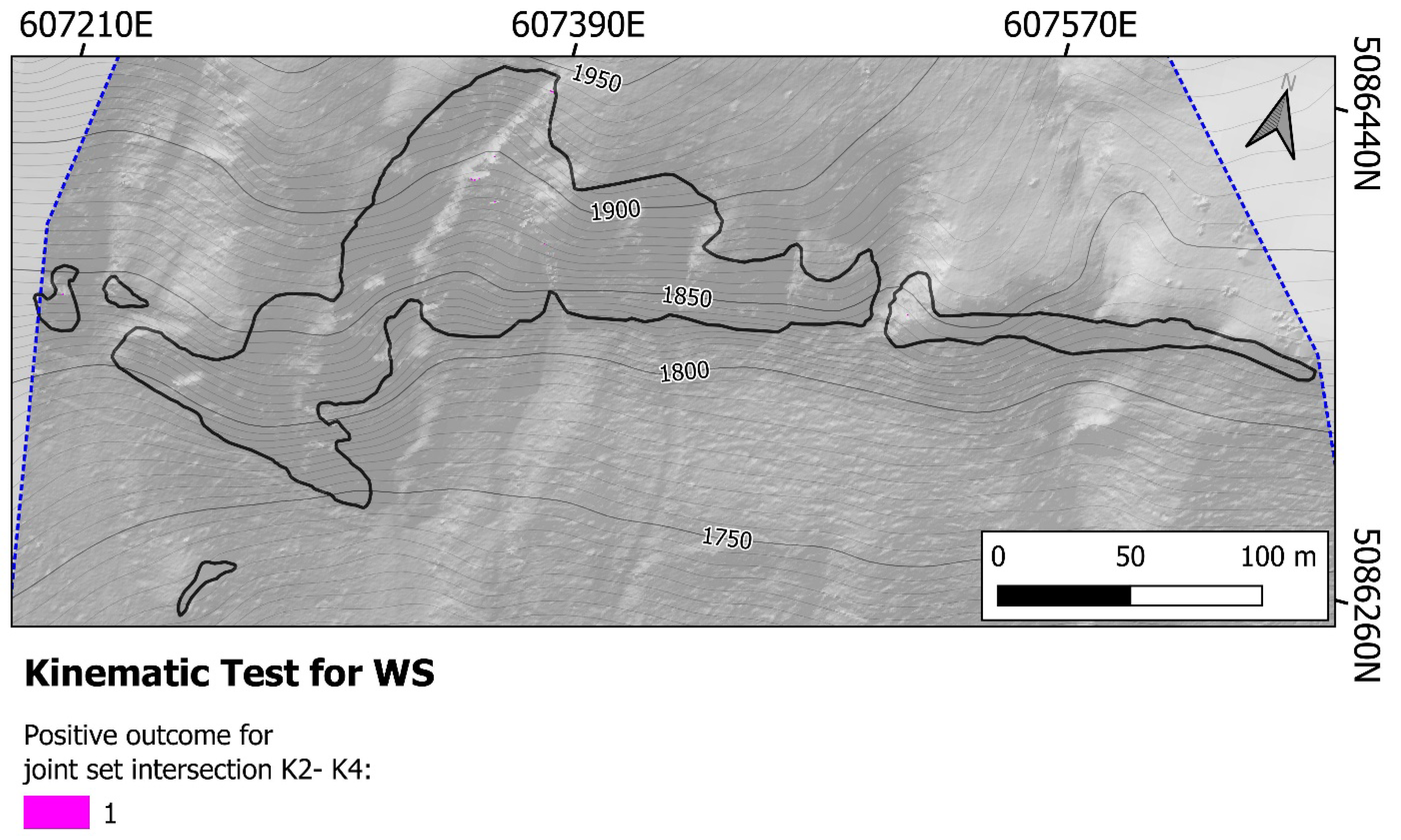
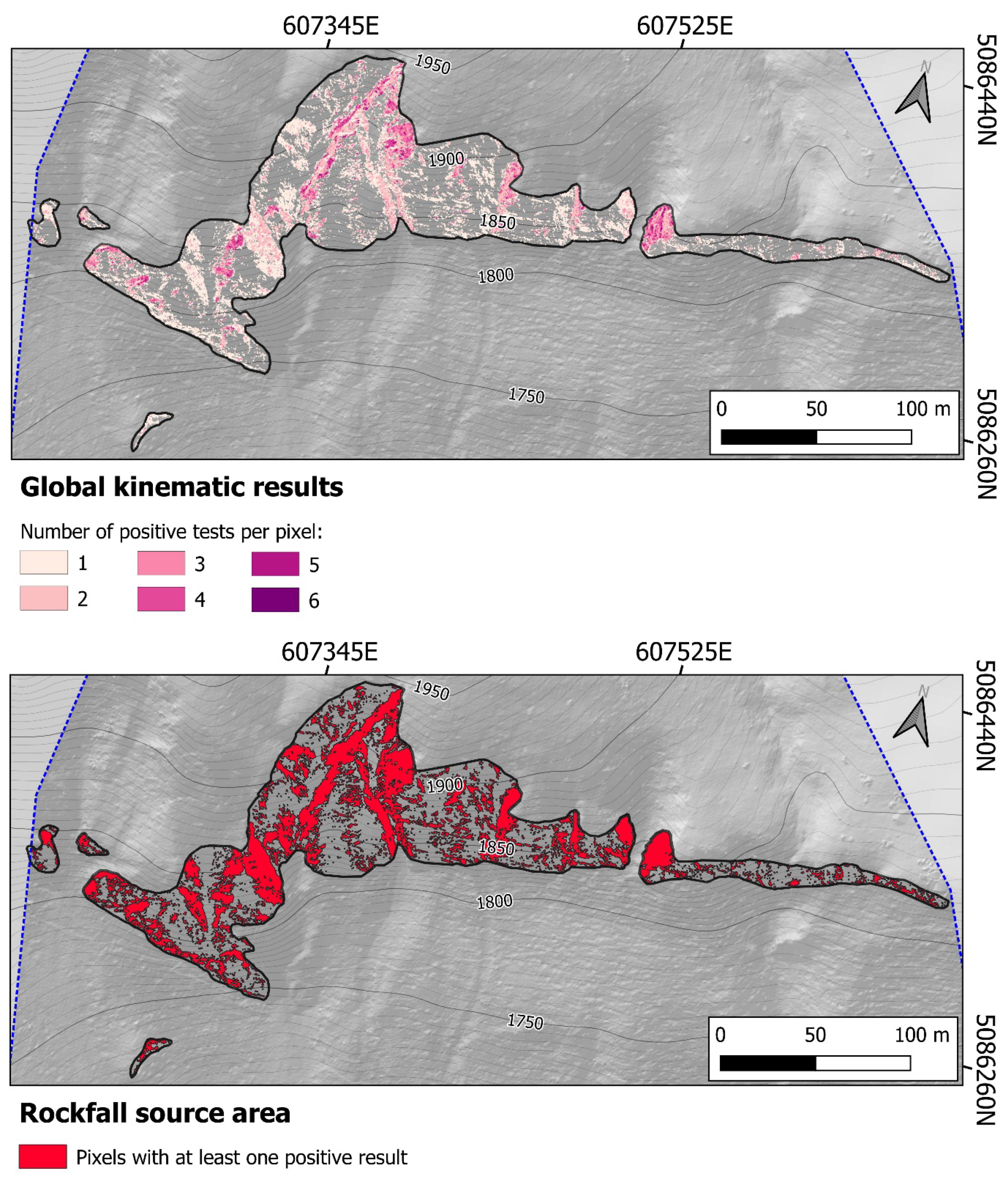
The last output file, the general sum image S (Figure 12, first half), gives a panoramic view of the kinematic conditions of the whole rock slope studied here. In general, large portions of the rock faces that characterize the upper part of the study area are prone to produce unstable blocks related to all three considered movement types. A critical portion of the rock faces allows at least one type of movement due to the widespread distribution of TP and WS. A significant portion of the rocky slope is prone to give at least two types of movement due to the significant overlap between the areas where PS and WS are geometrically possible. Lastly, along the westward exposed surfaces of the incisions that separate the rock faces, the highest scores can be found: up to six types of movement tested positive in the same pixel. The S matrix conveys two main pieces of information: first of all, where the critical sectors, i.e., those where a significant number of types of movement are possible at the same time, are located; secondly, it gives a general idea of how active a rock face can be and through which type of movement this activity is expressed. These pieces of information are of crucial importance when dealing with rock slope stability: the evident advantage of the algorithm presented in this paper is the possibility to appreciate these data spatially as maps.

The second half of Figure 12 shows how the data stored in the S image can be used to define source areas for 3D rockfall numerical simulations: by adopting this approach and taking advantage of the speed and ease of use of the algorithm, it is possible to precisely map source areas without employing simpler method such as defining the entirety of the mapped rock faces as source area. For example, for the rock faces of the case study site, approximately 40% of their area has been mapped as a potential source area: less than half of the complete rocky slope surface. Through our approach, it is possible to define as source areas only those portions of the rock face actually prone to produce movement and block instability. In light of these considerations, the proposed method could represent a powerful tool to improve efficiency in numerical simulations and, thus, in the process of rockfall hazard and risk assessment, protection works design, and implementation.

5. Conclusions

This work describes an algorithm that performs kinematic analysis employing as input data only a DTM of the considered rock face, together with orientation and friction angle for each of the joint sets surveyed in the rock mass. The goal was to introduce a quick and reliable tool based on current-day technology and data-gathering techniques, which could avoid the inherent problems associated with traditional stereoplot methods and approaches available in the literature. The algorithm philosophy and setup and the required input data were described; then, a suitable case study was selected to test the procedure and validate the results.

In all the three cases defined by the three main types of movement (PS, WS, and TP), the outputs of the algorithm were crosschecked with traditional Markland’s tests performed employing stereoplots, repeated for a sufficient number of slope configurations, with the same four joint sets used by the algorithm and defined through traditional geomechanical surveys performed on-site. In all three cases, the algorithm produced coherent results with what was expected by the traditional tests.

The tool proved to be reliable and useful, especially for studies and analysis related to rockfall hazard and risk assessment, protection work design, and implementation. This is especially true in those situations where large rock faces with articulated morphology are the object of study since the tool allows for the kinematic analysis of the entire rock face at once.

This new tool, and the approach behind it, still have limits. First of all, at the current state, it requires the definition of reference values for the joint sets of the rock mass; the algorithm cannot handle raw data sets and perform a probabilistic kinematic analysis. Secondly, it is true that using a DTM (or DSM) it is possible to overcome the limits of the traditional stereoplot method related to the need to simplify the geometry of the rock face, relying instead on a model of the actual rock face morphology. DTM and DSM have an implicit limit, though: they are 2.5D objects; namely, they store the tridimensional morphology (i.e., the elevation or z coordinate) on a 2D image. This means that it is impossible to analyze all those situations in which the rock face is concave; in these cases, a DTM should store more than one value of z at once, which is, by definition, impossible.

Although the algorithm simplifies the global process significantly, in the case of complex situations where the joints and discontinuity orientation vary considerably over the rock face, the need to divide the surface into homogeneous domains is still present, considering the deterministic approach followed by the algorithm presented here.

It should also be considered that at the current state, the algorithm does not perform direct toppling kinematic tests, which are planned to be implemented soon. At present, only flexural toppling is considered.

Lastly, it must be stated that when employing the algorithm presented in this paper, a local validation process should be performed, as it has been performed for the case study described in previous paragraphs. A small number of traditional Markland’s tests should be, therefore, performed on representative rock face orientations. This remains the only way to assess the soundness of the output of the algorithm.