Evaluation of Boulder Characteristics for Improved Boulder Detection Based on Machine Learning Techniques

Abstract

Detailed maps of the seabed and knowledge of its habitats are critical for a wide range of tasks, such as sustainable development, and environmental protection. Boulders on the seabed form an important environment for ecosystems, but the detection of them is challenging. In this study, we aim to improve the understanding of boulder predictors and to determine connections between predictors and boulder environments on different spatial scales. The Relief-F filter feature selection algorithm was used on four 30 m × 30 m areas in Rødsand lagoon, containing one boulder each, to determine the most relevant predictors. The predictors could be divided into four groups detecting different boulder characteristics: colour contrast, height, boulder boundaries, and spherical geometry. Twelve different types of boulder environments were evaluated. Bare, spherical boulders on sandy seabeds can be predicted from all four predictor groups. It is not possible to detect non-spherical boulders on seabed covered by vegetation. The best predictors for boulder detection depend on the shape and size of the boulder and the surrounding sediment and vegetation. The predictors were evaluated on a larger 400 × 2500 m area. When up-scaling the boulder detection area, larger seabed structures may affect the results. Therefore, knowledge about these structures can be used to remove errors and uncertainties from machine learning input data.

1. Introduction

Detailed maps and knowledge of the seabed and its habitats are critical for a wide range of tasks, such as sustainable development, and environmental protection ([1,2]). One of the essential habitats is stone reefs, that is considered important in the Habitats Directive (cf. Habitats Directive Annex 1 [3]). Boulders on the seabed constitute an important environment for marine animals to live, hide, and feed [4]. Additionally, marine spatial planning requires information about conditions on the seabed to assess the impact of offshore construction projects. Detection of boulders is also important for chart production for nautical information services [5]. An increased demand of habitat mapping on a larger scale, requires automation of the processing workflow in terms of accuracy, reliability, and reproducibility of the results [5]. Mapping of boulders is of great importance, but the identification process is challenging.

Boulders can be covered by vegetation, can be difficult detect due to reflections from the water surface, or they can be difficult to distinguish from other objects on the seabed. Studies have used experienced experts for manual interpretation of acoustical and optical data for the detection of boulders on the seabed and benthic habitats. These human interpretations have resulted in clearly differing results for the same data set ([2,5,6]). This poses a significant challenge both for the quantification of model performance of machine learning methods and for the establishment of correctly annotated training data sets [5]. In [2], manually classified maps had a lower degree of detail than maps created using automated classification. The automated classification recognized correct habitat separations, which were not indicated in manual classification. Some separations were not included in manual classifications due to doubts that arose during the interpretation process. Especially areas without clearly visible morphological boundaries introduce uncertainties in delineating the extent of a given bottom type [2]. These studies demonstrate the need for automated boulder detection.

Geomorphological characteristics of the seabed constitute a basic set of indicators of environmental conditions and their changes. [2].

Especially morphometric features (elevation, slope, aspect, planar curvature) are usually used as machine learning input in benthic habitat mapping ([2,4,5,7,8,9,10]). The difficulties in verification of habitat classes (boulders, seagrass, etc.), when creating training and test sets affects the performance evaluation of the algorithms. In ([2,4]), algorithms have detected habitats, which were not present in the test set. This could be due to errors or uncertainties in the algorithm, or there could be habitats which were incorrect classified in the test set. Machine learning algorithms use features to obtain connections between them and characteristics of the habitat, that need to be classified. When classifying points for a training or test set the classification is limited by the measurement technology used to obtain the data or by a definition, created by humans, of the habitats. It is possible that the machine learning algorithm detects connections between input data and habitat characteristics, which are not part of our description of that habitat. For boulders this could be material or height, but not size or shape. Therefore, the quality of input data is very important.

In [5], the authors conclude that the limiting factor for automated detection of boulders is not technology, but the domain knowledge and the availability of accurately annotated training data. Increased knowledge regarding seabed and boulder characteristics could deliver this information.

The best features for the automated detection of boulders (here referred to as predictors), can be determined by feature selection algorithms. There are three types of feature selection methods: filter, wrapper, and embedded feature selection [11].

Embedded and wrapper feature selection are adjusted to select the best features for a specific machine-learning method as in [4].

A filter type feature selection algorithm measures feature importance based on the characteristics of the features, such as feature variance and feature relevance to the response. In this case, important features are selected as part of a pre-data-processing step, and subsequently a model is trained using these selected features. Therefore, filter type feature selection is independent of the training algorithm [11]. Filter-based feature selection algorithms can evaluate feature performance using different parameters. Chi-square testing (${\chi }^2$) evaluates the correlation between two variables and determines whether they are independent or correlated [12]. It is used as a test of independence to evaluate whether the class label is independent of a particular feature in feature weighting ([13,14]). The Relief-F algorithm, introduced by [15], iteratively adjusts feature weights according to their ability to discriminate between neighbouring patterns [14].

In this study, we use the same data as in [4] to evaluate results from a feature weighting algorithm, independent of a specific machine learning method, to define boulder characteristics and to improve the input data for boulder detection. We aim to improve the understanding of boulder predictors and to determine connections between predictors and boulder environments (boulder and seabed appearance) on different spatial scales. The objectives are to identify the most important predictors for boulder detection, to evaluate the performance of each predictor, by using the relief-F feature selection method, and to determine which boulder characteristic the predictor scans for, and to evaluate the possibility of identifying boulders in different seabed environments, and on different spatial scales.

2. Study Site

Rødsand lagoon is located in southern Denmark between the islands of Lolland and Falster. There is a water exchange in the lagoon with the Fehmarn Belt in the western Baltic Sea to the south and through the narrow strait Guldborgsund with the inner Danish waters in the north (Figure 1). The lagoon is semi-enclosed by a barrier spit and two barrier islands [16] and has a size of 300 km². The water depths range between 4 m in the west and 8 m in the east. The lagoon is a protected Natura 2000 and Ramsar area [17]. Glacial processes during the Weichsel glaciation shaped the landscape of Lolland and Falster [18]. WNW–ESE oriented ridge and runnel morphology at the surface of the moraine landscape were aligned in the direction of ice shield propagation during the final stages of the glaciation. The seabed in Rødsand lagoon has a similar origin with ridge and runnel morphology and contains glacially deposited boulders. A number of sandy barriers formed on top of the elevated ridges of the drowned moraine landscape in the Holocene [19]. The seabed of the lagoon is subject to shallow marine and coastal processes. Wave processes form sandy barriers between the Rødsand lagoon and the open waters. The sediments are derived by wave-driven onshore transport of sand from the shoreface and from alongshore supply of sand from the adjacent coasts through littoral drift ([18,20]). The mean tidal range in the lagoon is 0.1 m (micro-tidal) and tidal currents are almost negligible. Basin-scale flushing and meteorological forcing drive the water exchange between the lagoon and inner Danish waters. This leads to water level fluctuations and causes flow circulation in the lagoon. The salinity of the water in the lagoon is brackish, about 10–20 PSU. This is due to exchange of brackish water from the Baltic Sea and salty water from Kattegat [21]. The fetch-limited waves in the lagoon are low to moderately energetic. Their bed shear stresses can cause erosion and suspended sediments in the water column. The layer of Holocene marine sediments in the lagoon is thin and reworked by wave-driven processes. This can bury boulders in some areas while exposing boulders in others. Marine seabed habitats in the lagoon include stone reefs and sandbanks. These form the physical foundation for flora like macroalgae and seagrass meadows. The marine habitats serve as food supply, homes, and hiding places for marine life. Stone reefs were mapped as part of marine habitat mapping of the inner Danish waters [22] and for the FEMA baseline study for the Fehmarn Belt Fixed Link [23].

3. Materials and Methods

3.1. LiDAR Survey at Rødsand in 2015

Topo-bathymetric LiDAR data were collected in Rødsand Lagoon on 7 September 2015 (Figure 1a), under clear sky conditions and with an average wind velocity of 6–7 ms⁻¹ (DMI, Weather archive). The company Air-borne HydroMapping GmbH (AHM) collected the data using a twin-engine aircraft (Tecnam P2006T) with a laser scanner (VQ-880-G, RIEGL LMS) integrated in the front of the aircraft, and with an internal measurement unit (IMU (IGI AEROcon-trol-IIe)) integrated on the top of this scanner. A compact GNSS (global navigation satellite system) antenna (NovAtel 42G1215A-XT-1-1-CERT) was mounted on top of the aircraft and constituted, combined with the IMU, a navigation system, that recorded the position and altitude of the aircraft at a rate of 256 Hz. The laser scanner emitted green laser pulses with a wavelength of 532 nm and a pulse repetition rate of up to 550 kHz. The flight speed was ∼80 kn (∼150 km/h), the point density was ∼20 points/m², and the altitude was 400 m. The laser beam footprint was ∼0.4 m due to a laser beam divergence of 1.1 mrad and the mentioned flight altitude. The laser scan pattern was circular, with a constant incidence angle of 20°, generating circular scanlines regularly shifted forward, resulting in a swath width of ∼400 m at this flight altitude. The typical water depth measuring range of the laser scanner is about 1.5 Secchi depth. The laser scanner system recorded full waveform data and intensity information was provided for each returned signal. The collected LiDAR data contained the following information: xyz coordinates, GPS time stamp, amplitude, reflectance, return number, and laser beam deviation ([24,25]).

3.2. Processing of Topo-Bathymetric LiDAR Data

The flight trajectory was calculated with the software packages Aerooffice and GrafNav and incorporated correction data of continuously operated GPS base stations. The software Riprocess from RIEGL LMS was, prior to the data collection, used to determine the boresight calibration parameters between IMU and the laser scanner, and later on used for strip adjustment [24]. The HydroVISH software developed by AHM, was used to remove water and noise points, which did not represent seabed or seabed structures, from the point cloud. The following attributes were computed for this process: classification, clustering (density), GPS time (time stamp), intensity, last return, number of returns, PointSourceID (strip number), positions (xyz coordinates), and return number. The dense seabed and habitat structures and the less dense water column points were clustered, using the point density attribute. Scattered points outside these clusters, especially below the seabed and above the water column were removed as flaw echoes. The density of the clusters was used to create a pre-classification to distinguish between seabed and water points. In this process, the clustered dataset was further divided into fragments to facilitate the data handling.

A triangular mesh that represented the water surface was generated using neighbourhood analysis, point density, and the water edge line. The latter was derived by creating the concave hull of the point cloud using alpha shape. Alpha shape is an algorithm, that creates a 2D shape of the outer points in a set of points [26]. Alpha shape creates a hull which takes the concave parts of the point shape into account, and therefore creates a more precise outline than a convex hull. The refraction correction for the remaining points below water was calculated using the water surface mesh after the removal of flaw echoes (see [24]). Refraction correction was necessary due to the difference in refractive index of air and water. The processed data resulted in a seabed point cloud, containing only points that constitute the seabed and structures or habitats associated with it. Each point in the point cloud has a corresponding value representing the intensity of the reflected signal. A workflow diagram showing the processing steps, described in the method sections, can be seen in Figure 2.

3.3. Single Boulder Detection

Morphometric features calculated from intensity, depth and geometry were evaluated through a filter feature selection algorithm in order to define the most relevant predictors for boulder detection. The features were calculated for a quadratic area of 30 m × 30 m with one boulder. This minimized signals from other boulders or noise. We repeated this procedure in four areas to avoid that the predictors were specific to one particular boulder appearance Figure 3.

Potential boulder positions were detected using ortho-photos from 2015 to 2019. Uncertainties in geo-referencing were taken into account by buffer zones surrounding each boulder. It was decided that the structures should be visible in at least four of the ortho-photos to represent boulders, otherwise the patterns were classified as vegetation or noise. The result led to the four boulders shown in Figure 4. Small dots representing boulders with a diameter of less than 0.4 m, which is the LiDAR footprint size limit, were not taken into account.

Some boulders could be partially covered by sediment, which could make them difficult to be detected by ortho-photos. The ability to recognize these boulders in ortho-photos depends on the boulder size and degree of vegetation coverage. The four detected single boulder areas are presented in (Figure 1c and Figure 3).

3.4. Features

Each point in the point cloud had one value for depth and one for intensity. These values were used to calculate 16 features for boulder detection. Three spectral features associated with the intensity of the reflected signal, seven positional features associated with the absolute and relative depths of the measured points, and six covariance features associated with how well different geometric shapes fit the measured points (see

Table 1. Feature overview.

Spectral Features	Positional Features	Relative Depth Features
Intensity	z	Linearity
Std intensity	Std z	Planarity
Mean intensity	Mean z	Sphericity
	dz	Omnivariance
	dp	Anisotropy
	Slope (plane gradient)	Change of curvature
	Azimuth

), were calculated for the four areas with single boulders.

The depth and the intensity values were taken directly from the LiDAR data, while the remaining 14 features were calculated for each point by using the point in combination with all points in the surrounding neighbourhood. The feature calculations were performed for a sphere, where six different search radii were tested: 0.5 m, 1 m, 2 m, 3 m, 4 m, and 5 m. The 0.5 m radius was the minimum radius due to a laser footprint size of 0.4 m. Furthermore, only points with at least four neighbouring points within the area of the radius were selected, otherwise they were excluded. However, no points were excluded due to the minimum of 5 points in neighbourhood (

Table 2. Neighbourhood point properties.

Neighbourhood	Min # of	Max # of	Average # of
Radius	Points in	Points in	Points in
(m)	Neighbourhood	Neighbourhood	Neighbourhood
0.5	5	31	16
1.0	22	103	78
2.0	86	392	306
3.0	191	859	671
4.0	332	1515	1157
5.0	495	2337	1753

).

The data were imported and visualized by the custom-built lasdata.m function in Matlab [27], and the feature extraction algorithm was inspired from the custom-built estimateNormal.m [28] function that used the built-in Matlab functions cov(), eig(), and KDTreeSearcher [4].

The LiDAR sensor recorded the signal amplitude of the returned echo. The intensity was the strength of the reflected signal [29]. The mean and the standard deviation of the intensity were calculated for all neighbourhoods (see [4]). The elevation z was measured with reference to the Danish Vertical Reference level (DVR90; mean sea level). The elevation change dz is the difference in z of the considered point and the lowest point in the neighbourhood. The standard deviation, mean and dz were computed for all neighbourhoods. The best-fitting plane of the neighbourhood was calculated from the neighbourhood points using the built-in Matlab function pcfitplane. The Matlab function pcfitplane fitted a plane to a point cloud that had a maximum allowable distance from an inlier point to the plane. The function returned a geometrical model that described the plane [30]. The distance used for this calculation was 0.1 m. The equation for the plane was determined by the pcfitplane equation:

$$ax+by+cz+d=0$$

(1)

The plane is constituted by the points $(x,y,z)$ which satisfy Equation (1). a, b, and c are the coordinates of a vector $\left(\begin{array}{c}a\\ b\\ c\end{array}\right)$ normal to the plane, and the constant d is given by $d=-\left(x_0,y_0,z_0\right)·\left(\begin{array}{c}a\\ b\\ c\end{array}\right)$, were $\left(x_0,y_0,z_0\right)$ is any specific point on the plane.

The distance $dp$ between the plane and a point $\left(x_1,y_1,z_1\right)$ in the point cloud, was then determined from the equation:

$$dp=\frac{|a{x}_1+b{y}_1+c{z}_1+d|}{\sqrt{a^2+b^2+c^2}}$$

(2)

The slope was determined as the gradient of the best fitting plane:

The planar equation can be written as

$$f(x,y)=z=Ax+By+C$$

(3)

with $A=-\frac{a}{c}$, $B=-\frac{b}{c}$, $C=-\frac{d}{c}$, so we have the gradient

$$\nabla f(x,y)=\left(\frac{\partial z}{\partial x},\frac{\partial z}{\partial y}\right)=(A,B)=-\left(\frac{a}{c},-\frac{b}{c}\right)$$

(4)

The slope is then

$$slope=\sqrt{A^2+B^2}=\sqrt{{\left(-\frac{a}{c}\right)}^2+{\left(-\frac{b}{c}\right)}^2}$$

(5)

The azimuth can be calculated from the slope as:

$$azimuth=si{n}^{-1}\left(\frac{slope}{\sqrt{slop{e}^2+1}}\right)$$

(6)

The geometrical distribution of the point cloud was investigated using tensor field analysis ([4,31,32]). The analysis was carried out by calculating the covariance matrix:

$$cov\left(A\right)=\frac{{\sum }_{i=1}^N(A_i-{\mu }_A)\times (A_j-{\mu }_A)}{N-1}$$

(7)

where N is the number of observations in the neighbourhood, A contains all observations in the neighbourhood, and ${\mu }_A$ is the mean of the observations. The covariance matrix was then diagonalized and the eigenvalues were calculated:

$$cov\left(A\right)·v_i=v_i\times {\lambda }_i$$

(8)

where $v_i$ is the eigenvectors and ${\lambda }_i$ is the eigenvalues, ${\lambda }_1$, ${\lambda }_2$, and ${\lambda }_3$ [4]. The eigenvalues were chosen so that ${\lambda }_1\ge {\lambda }_2\ge {\lambda }_3\ge 0$. The geometrical characteristics such as linearity, planarity, and sphericity were determined for each point in the point cloud from the following Equations [4,8,33,34,35,36]:

$$Linearity=\frac{{\lambda }_1-{\lambda }_2}{{\lambda }_1}$$

(9)

$$Planarity=\frac{{\lambda }_2-{\lambda }_3}{{\lambda }_1}$$

(10)

$$Sphericity=\frac{{\lambda }_3}{{\lambda }_1}$$

(11)

$$Omnivariance=\sqrt[3]{{\lambda }_1{\lambda }_2{\lambda }_3}$$

(12)

$$Anisotropy=\frac{{\lambda }_1-{\lambda }_3}{{\lambda }_1}$$

(13)

$$Changeofcurvature=\frac{{\lambda }_3}{{\lambda }_1+{\lambda }_2+{\lambda }_3}$$

(14)

The covariance features were calculated as in [4], but for all six neighbourhoods in the sensitivity analysis. All features outlined above were calculated for each point in each 30 m × 30 m point cloud and for all the six analysed radii in order to find out which features, and which radii, are best for displaying a boulder site.

3.5. Feature Selection and Predictors for Boulder Detection

The term “predictor” is here used for features with an associated neighbourhood radius that clearly identify boulders. The distribution of the values of a particular feature was compared with the known position of a boulder to determine the best predictors for boulder detection.

An objective measure to prioritize the features and thus determine the best boulder predictors was achieved by using a feature selection algorithm. This algorithm analysed the ability of the features to identify boulders using a data set with correctly classified points. A filter feature selection algorithm was chosen to ensure an objective result, independent of the chosen combination of calculated features. The feature values calculated for each point depend on the radius of the neighbourhood. If a point was less than 5 m from the boulder, the neighbourhoods with large radii included points representing the boulder. This means that there was a “boulder signal” at a point where there was no boulder. The feature thus had values near the area representing the actual boulder, which were larger than expected according to the classification data set.

The purpose of using larger radii, and thus more points, in the calculation of the features, was to even out spurious signals. Therefore, the features for larger radii often offered a clearer picture of the boulder. However, some filter feature selection methods, which evaluate how much the feature value for each point differs from the correct classification data set, would underestimate the degree of agreement between the pattern of the feature and the classification set, for larger radii. This would happen if the algorithm evaluates the feature from how much the feature value for each point differs from the correct classification data set. To overcome this difficulty, the Relief-F feature selection algorithm in Matlab was used to determine the important features and neighbourhood radii for boulder detection.

The Relief-F Feature Selection Algorithm

The Relief-F algorithm calculates a weight for each feature/neighbourhood combination, depending on the importance of the features. Instead of comparing the feature value of a point with the class of the corresponding located point in the classified test set, the comparison is made in a way which is independent of the physical location of the points. Rather than looking at how the feature-values deviate from each of the numbers given by the classification set, feature-values close to each other are used for the comparison. The algorithm determines the value of a feature for a point, and then identifies k other points whose values come closest to this value. It compares with the classification set and examines how many of these other points have the same class (boulder/non-boulder) as the point itself, and how many have a different class (hit and miss values). This procedure was carried out for all points and all features, and the algorithm now assessed how good each feature was at describing whether there was a boulder, using a calculated weight value (see relieff in [11]). If k is set too small, the estimates can be unreliable in case of noisy data, i.e., spurious data not reflecting actual physical conditions. On the other hand, a very large k can result in obscuring important predictors because of the increased probability of agreement between the values. To avoid these extremes, k was chosen as $\sqrt{X}$, where X was the number of observations in the data set. A boulder was represented by between 20 and 50 points, while $k=\left(about150\right)$ resulted in about 3 to 5 times as many investigated values. This creates a prediction error, because it increases the number of values deviating from the classification set. This error, however, is the same in all the feature evaluations, and will not, therefore, affect their relative ability to detect boulders. This larger value of k also ensures some robustness if an area includes a few boulder-like structures or boulders not recognized in the ground truthing process, where the four single boulders were found. If k were chosen as 10, which is sometimes recommended, a single boulder-like structure not included in the classification set could result in a good predictor being discarded. The algorithm was applied to each of the four single boulder areas (30 m × 30 m) and to the four areas together. The most relevant neighbourhood size was chosen for each feature and a threshold weight was chosen to select the features, which constituted the best boulder predictors. The sixteen features described in Section 3.4 were used for this analysis. The values for intensity and depth were used directly from the LiDAR data output, while the remaining 14 features were calculated for six neighbourhoods (0.5 m, 1 m, 2 m, 3 m, 4 m, 5 m), which led to 86 feature/neighbourhood combinations.

The choice of neighbourhood search radii will be discussed in Section 5.3.

The relevant features, each calculated with the chosen neighbourhood, were subsequently used to determine correlations between potential boulder environments and seabed morphology for larger areas.

3.6. Predictor Evaluation

The three feature categories, spectral features, positional features and covariance features, classify boulders from different perspectives. All categories identify ways in which the boulder differs from its surroundings. The spectral features are focusing on colour contrast and differences in material. Relative position features focus on height differences and differences in size between boulders and other structures on the seabed. Covariance features focus on the geometric shape of the boulders compared with the geometry of the rest of the seabed. Each predictor can predict boulder properties. The dominant predictor differs, depending on the seabed environment (seabed morphology, sediment type, vegetation, etc.).

We analysed the possibility to register the predictor signals in 12 boulder environments. We created these environments from knowledge about the appearance of boulders, and the environments they are found in, in Rødsand lagoon, but independently of the four boulders specific locations. Spherical and oblong boulders have been observed on orthophotos of the area, and there would be boulders half covered by sand, due to their glacial origin. Bare boulders and boulders covered by macroalgae were observed on photos from the area, and the seabed consists of eelgrass and sand [23]. A combination of these different boulder shapes, colour and seabed appearance was used to create these 12 boulder environments (see Figure 5).

We evaluated the predictors found in Section 3.5 and divided them into different boulder characteristics. Then an evaluation of the dominant characteristics for each of the 12 boulder environment was made.

4. Results

4.1. Important Predictors to Describe BOULDERS

All predictors are calculated for all neighbourhoods for each 30 m × 30 m single boulder area. The Relief-F algorithm computed the weight for all feature/neighbourhood combinations. All positive weight values are shown in

Table 3. Boulder 1 predictors with positive weight calculated from relief-F algorithm.

Features	Radius	Radius	Radius	Radius	Radius	Radius	Single
	0.5 m	1.0 m	2.0 m	3.0 m	4.0 m	5.0 m	Value
Spectral features
Intensity	0.0294	0.0294	0.0294	0.0294	0.0294	0.0294	0.0294
Std intensity	0.0334	0.0309		0.0001
Mean intensity	0.0208	0.0345	0.0238	0.0237	0.0193	0.0093
Relative position features
z	0.0402	0.0402	0.0402	0.0402	0.0402	0.0402	0.0402
Std z	0.1773	0.1899	0.0080		0.0100
Mean z	0.1010	0.0538	0.0003
dz	0.0520	0.0525	0.0443	0.0439	0.0414	0.0379
dp	0.0544	0.0330	0.0359	0.0277	0.0356	0.0300
Slope (plane gradient)		0.0474	0.0029		0.0035
Azimuth	0.0022	0.0478	0.0029		0.0035
Covariance features
Linearity	0.0060	0.0219
Planarity	0.0090	0.0220
Sphericity	0.1486	0.2231	0.0148	0.0097	0.0023
Omnivariance	0.0924	0.1260	0.0048
Anisotropy	0.1486	0.2231	0.0148	0.0097	0.0023
Change of curvature	0.1512	0.1706	0.0033	0.0044	0.0014

,

Table 4. Boulder 2 predictors with positive weight calculated from relief-F algorithm.

Features	Radius	Radius	Radius	Radius	Radius	Radius	Single
	0.5 m	1.0 m	2.0 m	3.0 m	4.0 m	5.0 m	Value
Spectral features
Intensity	0.0184	0.0184	0.0184	0.0184	0.0184	0.0184	0.0184
Std intensity	0.0506	0.0266
Mean intensity	0.0334	0.0111			0.0025	0.0001
Relative position features
z	0.0131	0.0131	0.0131	0.0131	0.0131	0.0131	0.0131
Std z	0.1105	0.0587	0.0465	0.0250	0.0068
Mean z	0.0355	0.0189	0.0188	0.0218	0.0157	0.0089
dz	0.0203	0.0153	0.0137	0.0151	0.0134	0.0121
dp	0.0159	0.0040	0.0134	0.0106	0.0077	0.0069
Slope (plane gradient)	0.0003	0.0087	0.0079		0.0013	0.0038
Azimuth	0.0021	0.0088	0.0079		0.0013	0.0038
Covariance features
Linearity	0.0238	0.0034		0.0216	0.0248	0.0230
Planarity	0.0242	0.0035		0.0216	0.0248	0.0230
Sphericity	0.0754	0.0735	0.0121
Omnivariance	0.0553	0.0443	0.0075	0.0006	0.0002	0.0003
Anisotropy	0.0754	0.0735	0.0121
Change of curvature	0.0650	0.0531	0.0072

,

Table 5. Boulder 3 predictors with positive weight calculated from relief-F algorithm.

Features	Radius	Radius	Radius	Radius	Radius	Radius	Single
	0.5 m	1.0 m	2.0 m	3.0 m	4.0 m	5.0 m	Value
Spectral features
Intensity	0.0253	0.0253	0.0253	0.0253	0.0253	0.0253	0.0253
Std intensity	0.0958	0.1251	0.0473
Mean intensity	0.0128	0.0044
Relative position features
z	0.0051	0.0051	0.0051	0.0051	0.0051	0.0051	0.0051
Std z	0.0260
Mean z	0.0130	0.0068
dz	0.0172	0.0156	0.0101	0.0017
dp	0.0133	0.0038	0.0064	0.0021	0.0246
Slope (plane gradient)			0.0103	0.0048		0.0055
Azimuth			0.0103	0.0048		0.0055
Covariance features
Linearity					0.0479	0.0481
Planarity					0.0479	0.0481
Sphericity	0.0151
Omnivariance	0.0170					0.0021
Anisotropy	0.0151
Change of curvature	0.0170

,

Table 6. Boulder 4 predictors with positive weight calculated from relief-F algorithm.

Features	Radius	Radius	Radius	Radius	Radius	Radius	Single
	0.5 m	1.0 m	2.0 m	3.0 m	4.0 m	5.0 m	Value
Spectral features
Intensity	0.0408	0.0408	0.0408	0.0408	0.0408	0.0408	0.0408
Std intensity	0.1949	0.1122	0.0036			0.0064
Mean intensity	0.1219	0.0196
Relative position features
z	0.0139	0.0139	0.0139	0.0139	0.0139	0.0139	0.0139
Std z	0.1805	0.0966
Mean z	0.0364			0.0048	0.0086	0.0103
dz	0.0188	0.0205	0.0205	0.0158	0.0290	0.0155
dp	0.0331	0.0363	0.0377	0.0223	0.0311	0.0452
Slope (plane gradient)	0.0001		0.0151		0.0032	0.0078
Azimuth	0.0040		0.0151		0.0032	0.0078
Covariance features
Linearity
Planarity
Sphericity	0.1376	0.0714	0.0109
Omnivariance	0.0720	0.0575	0.0001
Anisotropy	0.1376	0.0714	0.0109
Change of curvature	0.1277	0.0714	0.0049

and

Table 7. Predictors from all boulders with positive weight calculated from relief-F algorithm.

Features	Radius	Radius	Radius	Radius	Radius	Radius	Single
	0.5 m	1.0 m	2.0 m	3.0 m	4.0 m	5.0 m	Value
Spectral features
Intensity	0.0234	0.0234	0.0234	0.0234	0.0234	0.0234	0.0234
Std intensity	0.0668	0.0529	0.0111
Mean intensity	0.0403	0.0161	0.0001	0.0025	0.0038	0.0006
Relative position features
z	0.0152	0.0152	0.0152	0.0152	0.0152	0.0152	0.0152
Std z	0.1144	0.0736	0.0307	0.0145	0.0010
Mean z	0.0436	0.0215	0.0116	0.0107	0.0067	0.0029
dz	0.0241	0.0182	0.0179	0.0151	0.0146	0.0117
dp	0.0241	0.0078	0.0182	0.0076	0.0148	0.0135
Slope (plane gradient)	0.0003	0.0108	0.0114		0.0023	0.0008
Azimuth	0.0012	0.0109	0.0114		0.0023	0.0008
Covariance features
Linearity	0.0151	0.0032		0.0035	0.0142	0.0135
Planarity	0.0159	0.0032		0.0035	0.0142	0.0135
Sphericity	0.0833	0.0907	0.0152	0.0001
Omnivariance	0.0544	0.0504	0.0051
Anisotropy	0.0833	0.0907	0.0152	0.0001
Change of curvature	0.0754	0.0662	0.0078

and the best radius for each feature is marked in bold.

The weights for all 4 boulders are shown in Table 7, with the best radius for each feature in bold and the selected predictors in italics. The threshold value for predictor selection was set to 0.02 for the values in Table 7. The features in Table 7 with lower weight values, had very large variations in preferred radii for the different boulders.

The best predictors for boulder detection were determined as intensity, std intensity (0.5 m), mean intensity (0.5 m), std z (0.5 m), mean z (0.5 m), dz (0.5 m), dp (0.5 m), sphericity (1.0 m), Omnivariance (0.5 m), anisotropy (1.0 m), and change of curvature (0.5 m).

4.1.1. Spectral Features

The Relief-F algorithm results in positive weights in most of the spectral features and especially for small radii. Std intensity is the best spectral feature. The spectral features are especially good for boulder 3 and 4, where boulder 3 is best described with a neighbourhood radius of 1 m for std intensity and 0.5 m for mean intensity. Boulder 4 shows the strongest weights for the spectral features and is best described with a 0.5 m neighbourhood radius. Boulder 1 and boulder 2 get lesser weights and are best described by a 0.5 or 1.0 m neighbourhood radius. The spectral features measure differences in colour and structure on the seabed. Boulders in vegetation or with macroalgae coverage would obtain smaller weight scores than an unvegetated boulder on sand. This could be the reason for the difference in weight scores between boulder 3 and 4 compared to boulder 1 and boulder 2.

4.1.2. Relative Position Features

The Relief-F algorithm results in positive weights in most of the relative position features, especially for small radii. Std z is the best relative position feature and in fact the best of all features. z, slope, and azimuth have positive weights for all boulders, but the weights are too small to be counted as predictors for boulder detection. The other relative position features are especially good for boulder 1 and especially poor for boulder 3. Boulder 1 shows large weights for std z, mean z, dz and dp with a 0.5 m radius, even though a 1 m radius is better for std z and dz. Boulder 2 is best described with a 0.5 m radius for all four remaining features. Boulder 2 is also best described with a 0.5 m radius for std z and mean z, but a 4 and 5 m radius for dz and dp, respectively. Boulder 3 has very small weights, but is best described with a 0.5 m radius for std z, mean z and dz and a 4 m radius for dp. Z, slope, and azimuth would be good predictors on a flat, smooth seabed with a large uniform boulder. The poor performance in z, slope and azimuth is due to varying slope, vegetation, and variations of the seabed. Std z, mean z and dz can be affected by the variations of the seabed and the boulder size, which can cause differences in weights for each boulder. The preference of a large radius for dz and dp for some boulders may also be caused by many small variations of the seabed, which make the boulder signal disappear for small radii.

4.1.3. Covariance Features

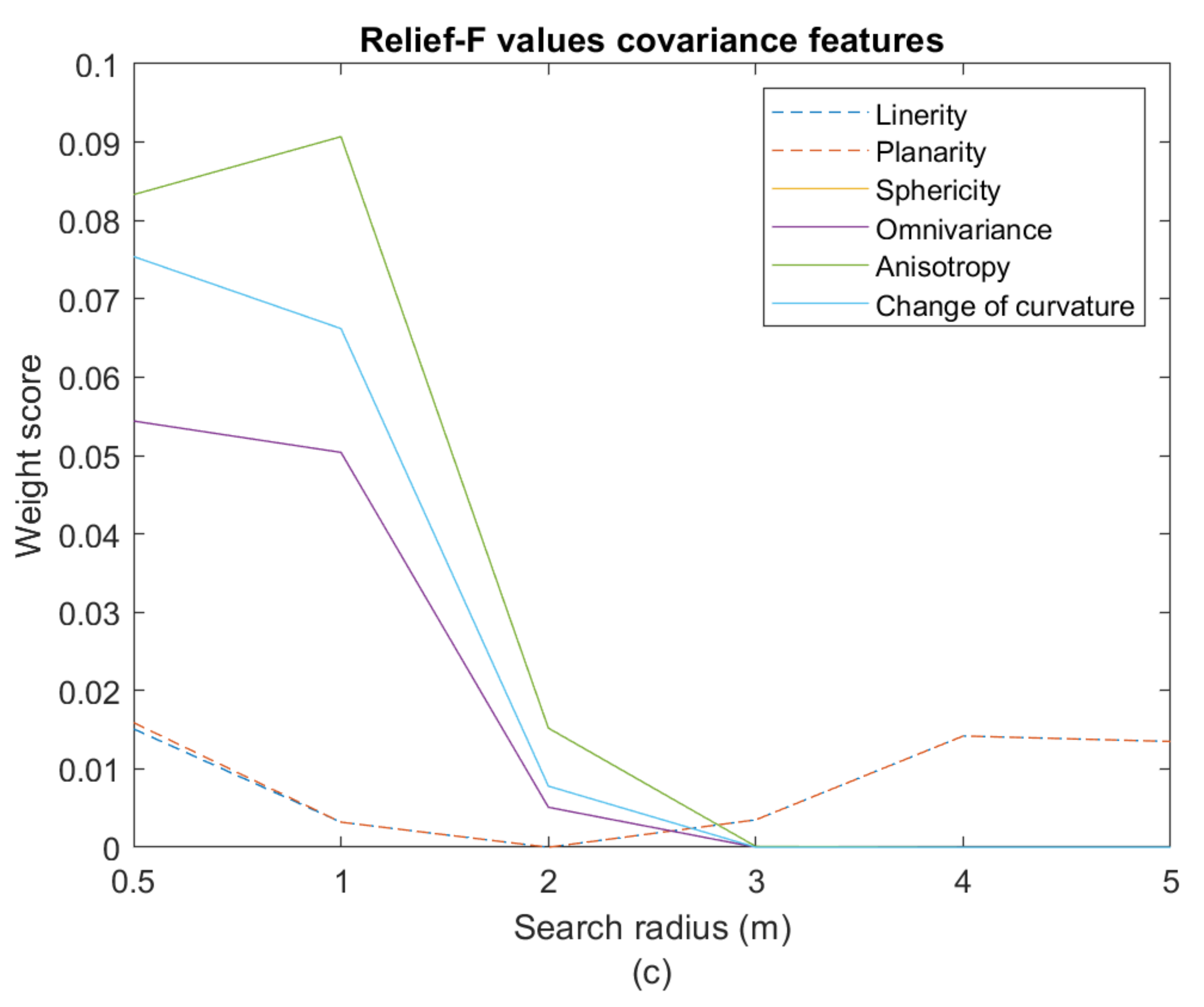
The Relief-F algorithm results in positive weights for most of the covariance features for at least one of the boulders. For the covariance features, the boulders vary a lot in the feature and radius combinations which leads to positive weights. The covariance features depend on the geometric shape of the boulder. For all boulders, small radii perform best for sphericity, anisotropy, omnivariance and change of curvature. Linearity and planarity have negative weights for many radii for each boulder, and the positive weights are too small for these features to be considered as predictors for boulder detection. This is because the appearance of a boulder is more spherical than planar or linear. Boulders are characterised by a low anisotropy signal, which implies that there is no preferred direction for the points constituting the boulder. Like a high sphericity, a low anisotropy implies that the boulder has a geometric form like a sphere. A high omnivariance also implies a spherical boulder, while the change of curvature detects differences in curvature between the boulder geometry and the seabed. The covariance features used are especially good for boulder 1 and especially poor for boulder 3. Boulder 1 is best described with a 1 m radius, but it also shows large weights for sphericity, omnivariance, anisotropy and change of curvature with a 0.5 m radius.

4.2. Boulder Characteristics

From the evaluation of each feature group, the predictors can be divided into four groups, each detecting different boulder characteristics. These characteristics are colour contrast (intensity, mean intensity, std intensity), height difference (std z, mean z), spherical shape (sphericity, anisotropy, omnivariance), and boulder boundaries (dp, dz, change of curvature). The appearance of the boulder and the seabed determines the success of each predictor group. In

Table 8. Predictor groups in different boulder environments.

Boulder	Colour	Height	Spheres	Boulder
Situations	Contrast	Difference		Boundaries
Spherical, bare, sand	x	x	x	x
Spherical, bare, vegetation	x	-	x	-
Spherical, macroalgae, sand	-	x	x	x
Spherical, macroalgae, vegetation	-	-	x	-
Flat or oblong, bare, sand	x	x	-	x
Flat or oblong, bare, vegetation	x	-	-	-
Flat or oblong, macroalgae, sand	-	x	-	x
Flat or oblong, macroalgae, vegetation	-	-	-	-
Partly covered, bare, sand	x	x	-	x
Partly covered, bare, vegetation	x	-	-	-
Partly covered, macroalgae, sand	-	x	-	x
Partly covered, macroalgae, vegetation	-	-	-	-

, the dominant boulder characteristics are evaluated for each of twelve boulder environments.

All four predictor groups are expected to detect large spherical boulders on bare sandy seabeds, while no predictor group are expected to detect non-spherical boulders covered by macroalgae on vegetated seabeds.

Standard deviation calculated for a neighbourhood with a small radius is the best way to locate boulders using the intensity and height data. Std intensity is a very strong predictor for locating bare boulders on a sandy seabed, but it would be ill-suited for locating macroalgae covered boulders in an eelgrass meadow. Std z measured for small radii is a very strong predictor for detecting large boulders on a flat seabed, but it would be ill-suited for distinguishing between boulders and other boulder-like structures, such as bedrock outcrops or small clusters of seagrass.

The dz and dp are good predictors for detecting the boundaries where large structures rise on a flat seabed, but they too would be ill-suited for distinguishing between boulders and other boulder-like structures. A high sphericity, high omnivariance and a low anisotropy are good predictors for detecting boulders if they are spherical. Flat boulders or boulders partly covered by sand, are difficult to detect from these predictors. Change of curvature is a good predictor for detecting objects with a curved appearance occurring on a flat seabed.

A grid with 0.5 m resolution, due to the 0.4 m footprint, has been created for each feature in Figure 6.

Table 9. Boulders represented in predictors. XXX means very clearly represented, XX means clearly represented, X means represented, - means not represented.

Features	Boulder 1	Boulder 2	Boulder 3	Boulder 4
Colour contrast
Std intensity	-	XXX	XXX	XXX
Mean intensity	-	X	-	XX
Intensity	-	XX	XX	XX
Height difference
Std z	XXX	XXX	-	XXX
Mean z	X	-	-	X
Spheres
Sphericity	XXX	XX	-	XX
Omnivariance	XX	XX	-	XX
Anisotropy	XXX	XX	-	XX
Boulder boundaries
Change of curvature	XX	XXX	-	XXX
dp	X	X	-	X
dz	X	X	-	XX
Boulder environments	Spherical, macroalgae, sand	Spherical, bare, sand	Partly covered, bare, vegetation	Spherical, bare, sand

shows whether each of the four boulders appears in the feature representation (Figure 6), which has resulted in an attempt to determine, which of the 12 environments each boulder represents. Boulder 1 cannot be seen in the colour contrast predictors, which is probably due to macroalgae covering. Boulder 3 can only be seen in the colour contrast predictors, which is probably due to non-spherical shape and vegetation cover. Boulder 2 and boulder 4 can be seen in all predictor categories and they are probably spherical, non-covered on sand.

4.3. Large Scale Analysis

The predictors were also estimated for a larger spatial area of 400 m × 2500 m (Figure 1b). Grids with 0.5 m and 50 m resolution were created for each feature (Figure 7) to investigate the boulder signals on a larger spatial scale.

Figure 6 shows whether a feature signal requires a high or a low predictor value to predict boulders. In Figure 7, clear predictor signals, low or high depending on what is required to detect boulders, can be identified in nearly the same area for all predictors. However, this signal can also clearly be detected in the 50 m × 50 m resolution, a resolution where single boulders should not be visible. The predictor signals could indicate a large representation of boulders in the areas, but knowing that it is difficult to distinguish between vegetation and boulders, we consider it more likely, that the signals are due to the presence of vegetation.

5. Discussion

5.1. Field Detection of Boulders

An investigation of the four boulders was carried out in October 2022, where boulder 1, boulder 2 and boulder 4 were recognized. There were no other boulders observed in the areas, that could have been detected by LiDAR. Since the field investigation was performed seven years after the data collection, permanent and temporary changes caused by boulder dynamics, storm events, erosion and deposition of sediments may have affected the area. These processes can have changed the degree of covering of the boulders, and vegetation patches.

The area was dominated by clayey sand, and included boulders ranging in size from 30 cm to 1 m. All observed boulders in the area were covered by macroalgae, while small patches of macroalgae were attached on cobbles. The boulder shape, sand cover and macroalgae cover and vegetation in the surroundings were investigated for the three detected boulders

Table 10. Boulder overview.

Boulder Number	Shape	Macroalgae Cover	Seabed Material
Boulder 1	Flat half covered	Covered by macroalgae	Sand with macroalgae patches
Boulder 2	Oblong	Covered by macroalgae	Sand
Boulder 3	-	-	-
Boulder 4	Spherical	Covered by macroalgae	Sand with macroalgae patches

.

According to Table 8 we conjectured that it would be more difficult to distinguish between a macroalgae covered boulder than a bare boulder. This was not the case for boulder 2 and 4, while boulder 1 is difficult to detect in the intensity values. An explanation could be that the colour contrast between bare boulder and sand and macroalgae covered boulder and sand are equally clear. However, the macroalgae covered boulder is more affected by surrounding vegetation patterns than a bare boulder, which could explain the low intensity values for boulder 1. The boulder shapes for boulder 1 and boulder 2 do not match the predicted shapes for boulder 1 and 2 in Table 9, but the reason is difficult to assess due to possible change in sand cover over time. Boulder 4 is predicted correctly except from some few patches of macroalgae Figure 8.

5.2. Feature Weight Values and Boulder Characteristics

The weight threshold value for the predictors has been determined for the analysis including all four boulders (Table 7). The value was chosen so that the discrepancy in preferred radius from boulder to boulder was at a minimum. It was set at 0.02 (Figure 9).

As seen in Table 3, Table 4, Table 5, Table 6 and Table 7, the weight values vary considerably from boulder to boulder. The values are not directly comparable, because the weight function used by the Relief-F algorithm depends on the number of data points and the ratio between the number of points in each class (boulder and non-boulder points). However, the internal differences in high and low feature values for each boulder and preferred radius can be compared. The large variations, from boulder to boulder, in positive weight values for the covariance features, could be due to differences between the geometric appearances of the four boulders. Boulders 1, 2, and 4 are described best with a 0.5 m radius for all four covariance features. Boulder 1 has very small weights for the covariance features, which could be due to large structures on the seabed similar to the boulder. This could be clusters of macroalgae, similar in size to the detected boulders, but only growing on small cobbles. The large weights and preferred 1 m radius for boulder 3 could be due to the size of the boulder, which is much larger than the other three. The spectral features have large weights for boulder 3 and 4 and small weights for boulder 1 and 2. The spectral features measure colour difference, which could imply structures on the seabed in the areas with boulder 1 and 2 with similar colours as the boulders. This could be macroalgae-covering of the boulder and similar vegetation in the area, or just that the boulders are placed on a vegetated area. The colour contrast between boulders and seabed is more clear for the areas including boulder 3 and 4.

5.3. Choice of Search Radii for Boulder Detection and Habitat Mapping

Only the smallest search radii in the neighbourhood analysis were used to define the best predictors. The analysed boulder search radii are chosen according to the definition of boulders in the Udden-Wentworth grain size classes. A boulder is defined to be between 0.25 m and 4.1 m in diameter. The 5 m search radius is chosen to ensure a radius, so that the boundary between boulder and seabed can be registered for all points of a 4.1 m boulder. Neighbourhood analysis with search radii from 0.2 m and up to 5 m would therefore be preferable.

However, the data collected in this study are limited by the LiDAR footprint size of more than 0.4 m. A search radius smaller than 0.5 m would therefore not be relevant. The four boulders in the study area are all smaller than 1 m in diameter, so an analysis of larger boulders would probably lead to larger preferred neighbourhood radii.

In [37,38], cobbles and boulders are detected from side scan sonar data in different resolutions (0.08 m, 0.2 m and 0.4 m). These studies make it possible to detect very small stones, but a smaller search radius would be required to create an automated detection algorithm with the high data resolutions used in these studies. Detection of cobbles and boulders with this resolution can result in valuable knowledge related to stone reef conservation and reconstructions. In [38], a higher biodiversity richness was found on a collection of small boulders, than the biodiversity richness on a single large boulder representing the same surface area as the small boulders. Therefore, small-scale investigations are very important.

5.4. Predictor Identification on Larger Scale

On the large scale evaluation (in Section 4.3), the signals represent a very large area, and are therefore more similar to vegetation patterns, than to signals from sporadically positioned boulders. The bottom vegetation map, based on results from an aerial photo survey and results from video recordings along transects in 2009, presented as Figure 2.9 in [23], shows vegetation patterns in the area corresponding to the signal found by the large scale predictors. If we assume that the large signals in the predictors are due to vegetation, the boulder signal disappears when up-scaling. To be able to detect boulders on a large scale on the areas not affected by vegetation, the vegetation areas need to be known and the vegetation signals need to be removed from the data.

Similar issues are discussed in [5], where morphological features related to bottom trawling create steep local and almost circular patterns similar to small boulders in slope maps. It is also seen in [2], where the automatic classification is affected by the direction of the bathymetric and sonar measurements. These two studies recommend these kinds of visual artefacts are manually removed from the data before the automatic interpretation is performed. On some of the feature visualisations in this study in Figure 6 and Figure 7, circular patterns originating from the rotating wedge prism scan patterns from the LiDAR instrument, can be seen in the data. However, on Figure 6 and Figure 7, it seems that the predictor values depend much more on the seabed structures than on the LiDAR scan patterns.

Other large-scale patterns, which could affect the data, could be large-scale morphology on the seabed like ridges, swales, inlets, or basins. These patterns can affect the predictor performance. If the large-scale patterns are known, they can be removed from the data before predictor calculation as in [2,5].

Sometimes it can be difficult to remove patterns that originate from noise from the survey, other habitats, or morphology. Instead habitats or structures with similar characteristics could be handled by the calculation of a specific feature or a new data representation, adjusted to distinguish between them. In [37], images with three different resolutions were generated, which made it possible to differentiate between cobbles and boulder signals. We chose to describe the situations with spherical and non-spherical boulders, macroalgae-covered or bare boulders, on a seabed consisting of sand with or without vegetation cover. These situations were chosen due to the conditions in Rødsand lagoon. However, there are relevant factors which could also be considered, such as other large-scale structures, like offshore sandbanks, or small-scale irregularities, like mussel or oyster patches, on the seabed.

5.5. Level of Detail in Classification

In Section 3.6, we investigated three boulder types in different environments. This resulted in 12 boulder situations. The appearance of the boulder, and the environment that surrounds it, can be described by many different factors. When we evaluate each boulder situation, we can develop tools and approaches to detect boulders in this specific situation. The number of factors considered to describe the situation affects performance. Predictors adapted to a very specific situation will be good at detecting boulders in this particular situation, but less suitable for describing new situations. Therefore, the choice of factors is relevant for the detection performance.

For automated detection of boulders, the choice of the input data is crucial, and it is affected by the seabed environment, which is mapped. The input data can be adjusted to a very specific boulder size, shape, or seabed environment, which results in better performance scores for detection of this specific situation. The input data can also be adjusted to a larger area with more variation, but with more generalized results, but worse performance scores. A clear definition of the aim of the investigation is necessary to improve input data. Knowledge about seabed morphology, other habitats, and specific boulder appearance of the area, can be used to choose machine learning predictors and data type and resolution. Point cloud data results in 3D features, which makes it possible to distinguish between circles and spherical boulders on the seabed, while a method to distinguish between boulders in vegetation still is needed. Partly covered boulders on sand can be detected from colour difference from LiDAR intensity, but vegetated patches in the surroundings will remove this signal. It is therefore important to combine a specific set of predictors designed to distinguish seabed morphology and habitats, adjusted to the relevant area.

6. Conclusions

We found that boulders can be detected from four different boulder characteristics: Colour contrast, height difference, spherical shape, and boulder boundary. Colour contrast can be detected from intensity features, height difference from std z and mean z, spherical shape can be detected from sphericity, omnivariance, and anisotropy, while boulder boundaries can be detected from change of curvature, dp, and dz. The best predictor from each of the four groups was std intensity, std z, sphericity and change of curvature, all calculated with a neighbourhood search radius on 0.5 or 1 m. Unvegetated, spherical boulders on bare sandy seabed can be detected from all four boulder characteristics, while unvegetated boulders, partly covered by sand, on bare sandy seabed, can be detected from height and colour contrast predictors.

Spherical, boulders, covered by macroalgae on bare sand can be detected from all four groups of boulder characteristics, but even very small patches of vegetation or macroalgae growing on cobbles can affect the colour contrast signal. It is difficult to detect boulders in vegetated areas, especially if they are non-spherical.

Pre-knowledge about the dominating boulder environments in an area could lead to better input data for machine learning. When up-scaling the boulder detection area, larger seabed structures may affect the results. Therefore, knowledge about these structures can be used to remove errors and uncertainties from the machine learning input data.

Larger studies of habitat characteristics and discriminators between habitats and seabed structures will be useful when improving automated boulder detection.