Abstract
(1) This article is devoted to the development of a theoretical and algorithmic basis for numerical modeling of the spontaneous potential method (SP) as applied to the study of sandy-argillaceous reservoirs. (2) In terms of coupled flows, we consider a physical–mathematical model of SP signals from an electrochemical source, with regards to the case of fluid-saturated shaly sandstone. (3) An algorithm for 2D finite-element modeling of SP signals was developed and implemented in software, along with its internal and external testing with analytical solutions. The numerical SP modeling was carried out, determining the dependences on the reservoir thickness and porosity, the amount of argillaceous material and the type of minerals. We performed a comparative analysis of the simulated and field SP data, using the results of laboratory core examinations taken from wells in a number of fields in the Latitudinal Ob Region of Western Siberia. (4) The results of the study may be used either for the development of the existing SP techniques, by providing them with a consistent computational model, or for the design of new experimental approaches.
1. Introduction
Over the last decade, there has been a significant technological development of logging equipment for geophysical surveys in oil and gas wells. High-precision devices for synchronous wireline logging in one trip in vertical wells were created, as well as autonomous complexes for logging on drill pipes in highly deviated wells. Among a large number of geophysical methods implemented in modern equipment, one of the most demanded in the study of geological sections and widely used in all drilled wells is the method of spontaneous polarization potentials (SP).
SP logging consists of the recording along the wellbore of electrical signals arising naturally due to physical and chemical processes occurring in the near-wellbore space [1,2,3]. SP sources include electrokinetic [4,5,6], electrochemical [7,8] and redox processes [9,10]. Despite the long history of the SP method, it still remains the key method for studying geological sections exposed by oil and gas wells in order to identify reservoirs, quantify their filtration-capacitive properties, namely porosity, sandiness, salinity of formation water, etc. [11,12,13,14].
With all the development of computational technology, correction charts remain the main tool for analyzing SP logs. These are calculated using equivalent electrical circuits and analytical solutions in simplified formulations [1,15,16]. Correction charts allows one to determine the value of static spontaneous potential (SSP) as an electromotive force, under the action of which electric currents circulating in and near the borehole arise. It is assumed that the region of the borehole adjacent to permeable formation is electrically isolated from the rest of the borehole. As a result, SSP depends only on the ratio of salinity of the drilling mud filtrate and of the adjacent formations (and, analogously, the ratio of the resistivities of the drilling mud filtrate and formation water). However, this closed-circuit approach does not fully reflect the physical and chemical processes leading to SP formation [17,18]. To fully describe the physical and chemical processes occurring in the near-wellbore space, it is preferable to use the theory of coupled fluxes and nonequilibrium thermodynamics [17,19] and apply numerical methods to solve differential equations describing the formation of SP signals [20,21,22]. In this connection, one of the most important tasks today is the application of modern methods of computational mathematics and the development of efficient computational algorithms and computer programs [23,24] allowing the simulation of spontaneous polarization potentials in a class of realistic models that adequately reflect the experimental conditions [25,26,27,28]. To date, a number of approaches for the simulation of SP logging data based on the finite element method (FEM) have been proposed [29,30,31].
We propose an algorithm for numerical simulation of SP logging data in an axisymmetric model of a fluid-saturated sandstone reservoir in between shale sediments. A physical–mathematical model of a clayey sandstone reservoir is used, which takes into account both the clay material content and the type of clay minerals. Numerical solution of the forward SP logging problem is performed in a two-dimensional formulation and is based on the finite element method with approximation of electrophysical parameters by sigmoidal functions. The developed algorithm is tested with successful reproduction of analytical results obtained in approximation of infinitely extended dipole layers [2]. The computational algorithm is used to numerically simulate SP signals with the establishment of their dependencies on model parameters. The capabilities of the algorithm are demonstrated on field SP logging data using the results of laboratory studies of core from intervals of the Lower Cretaceous deposits, penetrated by wells in a number of Western Siberian fields.
2. SP Problem Statement
2.1. The Description of the Physical Model
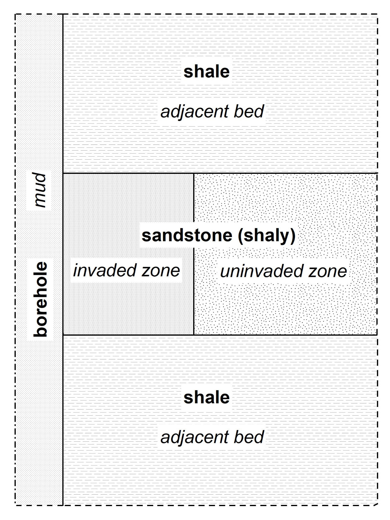
The SP problem is considered in a two-dimensional geological model, including a permeable sandstone bed and adjacent impermeable shale deposits (Figure 1). A constant element of the model is a well, the boundary of which is described by a cylindrical surface. When the permeable formation is penetrated, fresh water-based mud filtrate penetrates the medium, forming a zone with changed fluid saturation outside the well—the zone of drilling mud filtrate invasion [32,33].
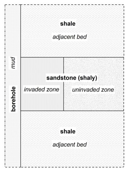
Figure 1.
Model of a reservoir formation (sandstone) with an altered near-borehole zone in-between shale sediments.
The correct description of the SP phenomenon from the basic physical principles is carried out with the help of the coupled fluxes formalism. The coupled fluxes are understood as a combination of conduction current, caused by the presence of an electric field in the medium, and charged particle current caused by physical and chemical processes of different nature occurring in the near-wellbore area [18,19,31]. The density of the total volumetric current flowing in the medium is represented as a sum of two components:
where is the volumetric conduction current and is the volumetric current of the SP source.
These source currents are caused by the presence of ion activity gradients, filtration of drilling mud and formation water, as well as redox processes. In this case, the divergence of the total volumetric current density is assumed to be equal to zero, which is equivalent to the requirement of conservation of the total charge in the medium:
Expressing the conduction current density through the electric field in the medium () and introducing its scalar potential (), we obtain the Poisson equation of the SP problem:
where is the electrical conductivity of the medium and is the scalar potential.
The resulting equation defines the electrostatic potential distribution for an arbitrary source of SP that induces an external current, .
In this paper, the contribution of ion activity gradients, also called the electrochemical current source, is considered as such a SP source. Since the other two contributions to the formation of SP, namely caused by drilling mud/formation water filtration and redox reactions, are much smaller than the contribution of ion diffusion, in most cases they can be neglected. The expression for the current density of an electrochemical source can be derived from the basic principles of ionic diffusion in charged porous media. Here we utilize the approach presented in [2], according to which the current density of an electrochemical source can be determined as:
where and are the diffusion and diffusion–adsorption EMF coefficients, respectively, is the diffusion–adsorption activity of rock and is the electrical conductivity of the fluid, depending on the concentration of ions at a given temperature. Given the definition of the source current density (4), the Poisson Equation (3) takes the following form:
where and are the corresponding values of electrical resistivity.
2.2. Accounting for Shale Content
It is well established that in the case of pure sandstone with a non-conductive matrix, the resistivity of the formation and the resistivity of the fluid saturating it are related by the Dakhnov–Archie relation [34,35]. However, this empirical model does not take into account a number of factors, including shale material, the content and type of which significantly affects the overall resistivity of the medium. Although using the description of the problem (5) automatically accounts for the shalyness of the formation, when a proper constant is taken, it does not allow to separate the effect of shalyness from other contributions to the resulting SP.
To correctly account for the effect of clay material content and type on the SP signal in the case of a clayey reservoir (Figure 1), it is necessary to use the parameterization, in which the values of and in Equation (5) are redefined as follows. Thus, the diffusion–adsorption EMF coefficient can be represented in the following form:
where is the macroscopic Hittorff number (transfer number for cations), is the Boltzmann constant, is the temperature, is the elementary charge. The macroscopic Hittorff number for cations reflects the fraction of electric current in the porous medium carried as a result of cation transport, and can be expressed through the petrophysical properties of the formation as follows [17,31]:
where is the porosity, is the water saturation, is the effective mobility of cations on the mineral surface, is the solid phase density (2650 kg m−3 for silica), is the cation exchange capacity and is the microscopic Hittorff number (0.4 for NaCl solution), determined by the relative mobility of cations in the free electrolyte solution. Using these values, we can also obtain an expression for the reservoir resistivity in the following form:
where is the cementation exponent and is the saturation exponent. This expression takes into account the contribution to conductivity from both formation water resistivity (Dakhnov–Archie law) and the effect of surface charges of clay minerals present in the formation (Waxman-Smits model) [36]. The magnitude of the latter is determined mainly by the cation exchange capacity. If the sandy reservoir contains clay minerals, it is necessary to use the average cation exchange capacity [17]:
where is the clayiness, is the cation exchange capacity of sand and is the cation exchange capacity of shale.
3. Forward SP Modeling
3.1. Finite Element Method Computation
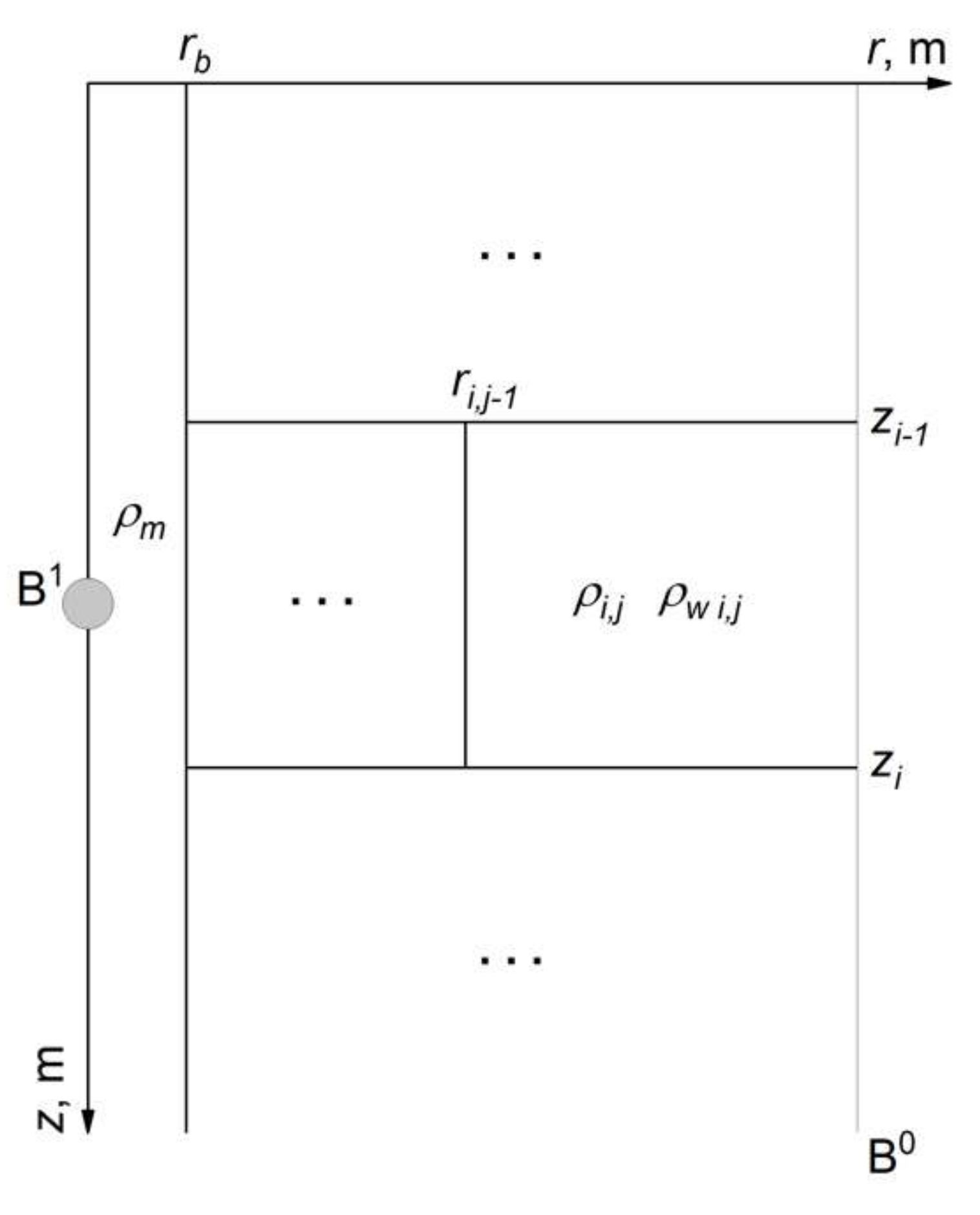
The model of the geological medium shown in Figure 1 is axisymmetric, considered in the cylindrical coordinate system . In general, the model may include a bundle of formations with plane-parallel horizontal boundaries, with several radial zones in the near-wellbore area of each permeable formation separated from the well and from each other by coaxial–cylindrical boundaries (Figure 2).

Figure 2.
Axisymmetric model of the geological medium. Notations: —radius of the well, —resistivity of the drilling fluid, —resistivity of the j-th radial zone of the i-th formation, —resistivity of the fluid of the j-th radial zone of the i-th formation, —radius of j-1-th radial zone of the i-th layer, —coordinate of the i-th layer top, —coordinate of the i-th layer bottom, B0—outer boundary of the area, B1—surface of the measuring electrode.
In Equation (5), for each value of , the diffusion–adsorption EMF coefficient is a constant value, while and are functions of and take different values in the well and formation. The values of the functions and may be different in each of the radial zones of the near-wellbore area, while in the borehole they are taken the same and equal to the drilling fluid resistivity . The solution of the forward SP problem is based on the calculation of the electric potential distribution in the investigated area using Equation (5) with a given distribution of functions , and parameter .
A numerical algorithm based on FEM is proposed for modeling SP logging data. The use of FEM makes it possible to effectively calculate the electric potential distribution in logging problems both in the case of axial symmetry and three-dimensional geometry [37]. Here the FEM is used to solve the partial differential Equation (5) within an axially symmetric region. The boundary conditions and the right-hand side of the equation are set and, importantly for the calculations, the parameters of the grid of the computational domain are determined and selected.
The electrode used to record signals during SP logging can be considered a sphere of small radius. The size of the electrode is much smaller than the borehole radius and its influence on the values of recorded signals is insignificant. The first boundary condition is that the normal component of the electric field on the electrode surface is zero, which is equivalent to the vanishing of the potential derivative along the normal:
where B1 is the electrode surface. Additionally, a necessary boundary condition is that the potential at the distance from the current sources is equal to zero:
where B0 is the outer boundary of the modeling area. The choice of the size of the outer boundary is dictated by the requirement of zero potential and at the same time the need to provide an optimal calculation time.
Consider a two-dimensional region , in the general case with inhomogeneous distribution of physical properties, on which we define the following functional spaces:
where is a Lebesgue space for the elements of which scalar product can be introduced:
The Equation (5) in the general form is, as follows:
In order to use FEM to solve Equation (14) with boundary conditions (10) and (11), we turn to a variational formulation of the boundary problem. This requires finding a function for which any holds:
This formulation of the problem automatically leads to the fulfillment of boundary conditions (10) and (11). To find an approximate solution of the variational problem, we will use the basis function expansion, the set of which forms a finite-dimensional subspace of the space :
where is the i-th basis function and is its weight in decomposition.
For an approximate solution, the variational problem becomes discrete and takes the following form:
Find such that holds
At the same time, since any function can be represented as a basis function expansion of a given subspace, it is sufficient to require (17) only for all given basis functions, which leads to a set of N equalities of the following form:
This expression can be rewritten in matrix form:
where is a vector of weights of basis functions uniquely determining the required approximate solution. Thus, the problem of finding the electric potential is reduced to the search for the solution of the system of linear Equation (19), the coefficients of which are defined by the following expressions:
Since the SP problem is two-dimensional in the axial symmetry approximation, the bilinear functions defined on a rectangular grid were chosen as basis functions. To find the solution of (19) the Kholetsky decomposition was used. This is due to the fact that the resulting matrix is positively definite and can be easily reduced to the symmetric form.
3.2. Determining Source Current Density
To determine the function of the right-hand side of Equation (14), it is necessary to specify the distribution of current density of external sources, or, similarly, the resistivity, as well as the parameter as a function of spatial coordinates . Since the functions and take different values inside the well and inside each of the radial zones of the reservoir (Figure 2), they can be represented as piecewise constant on and stepwise on functions of the following form:
where is the radial function of the resistivity for i-th formation, depicted in Figure 2, is the resistivity of the fluid, is the resistivity of the j-th radial zone of the i-th formation, is the Heaviside function, is the radius of j-th radial zone of the i-th formation, –number of radial zones in the i-th formation and is a number of formations. A similar expression can be written for .
Since the analytical calculation of the right-hand side of Equation (14) requires finding the gradient of as well as finding the gradient and divergence of sequentially, the corresponding functions must be sufficiently smooth. Since the Heaviside function is not smooth, this approximation is not applicable. In this connection, the approximation of the radial resistivity functions with sigmoidal functions of the following form is used:
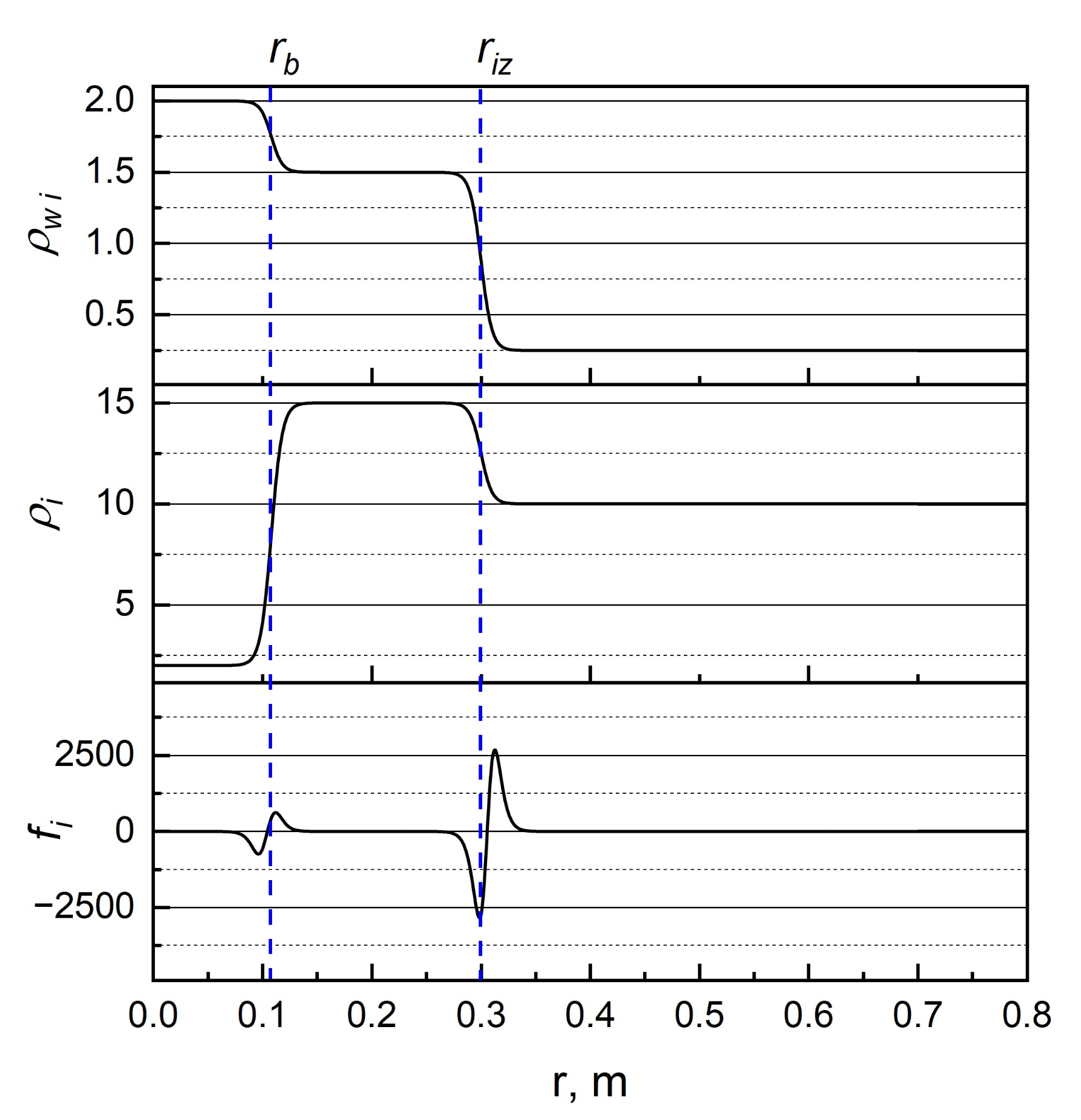
where parameter determines the slope of the sigmoid, or the size of the transition region between adjacent zones. This transition region is a consequence of approximation of the initial piecewise constant function and does not reflect real transients between the well and the formation. In the limit -> ∞, Equation (22) turns into (21). An example of the resulting form of the function of the right part for the i-th formation when setting the radial functions and by the method described above is shown in Figure 3.
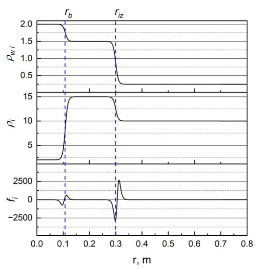
Figure 3.
Characteristic view of the functions and , given by Equation (22), and the corresponding function for the -th reservoir. The model of the medium includes a well with a radius of 0.108 m and a permeable formation with an invasion zone of radius 0.3 m. The slope parameter of the sigmoid A is taken to be 200, and the value of = −11.6 mV. The dashed lines show the vertical boundaries of the well and the invasion zone.
To calculate the elements of the system of linear equations, it is necessary to calculate integrals from the obtained function on the finite element grid of the form (20). Since the function changes rapidly near the wellbore boundary, the Simpson method with an adaptive integration step is chosen for numerical integration. In this approach, the number of partitions of the integration interval is doubled until the difference of integral values calculated at the current and the previous step becomes less than the specified value. In this case, the function values calculated at the current step are used to calculate the following iterations, which reduces the computational cost. Despite the fact that Simpson’s method is usually less efficient than some other methods of numerical integration (e.g., Gauss method), in this case its usage allows us to dispose of the procedure of integration grid setting. This simplifies the software implementation of the algorithm, in particular, when varying the mesh of finite elements or values of simulation parameters.
4. Results and Discussion
4.1. Testing the Computational Algorithm
To test the developed algorithm, simulation of SP logging data was performed on several typical examples. A particular case of the geoelectric model shown in Figure 2 includes a well, a formation of clean fluid-saturated ( = 1) sandstone without an invasion zone and the adjacent layers of shale sediments. In the well, the function takes the mud resistivity , while in the permeable reservoir it takes the sandstone reservoir resistivity . The value of the function in the well, as well as for the function , is equal to , and in the reservoir to the resistivity of formation water . The diffusion–adsorption EMF coefficient in the limiting case of pure sandstone is −11.6 mV, while in shale sediments it takes the value of 58 mV. The simulation parameters used in testing the computational algorithm on all examples are shown in Table 1.

Table 1.
Parameters of the sandstone bed model in the adjacent shale sediments used in the numerical simulation.
By selecting a sandstone formation in which thickness is many times greater than the borehole radius, it is possible to obtain a SP logging curve close to the static SP curve. To match the model case of static SP, the resistivities of the adjacent formations and reservoir are assumed to be equal to the resistivity of the drilling mud. Calculated at different values of SP anomaly amplitude this approximation agrees with the equation describing static SP (Figure 4): , where is the static SP coefficient, in this case equal to 69.6 mV.
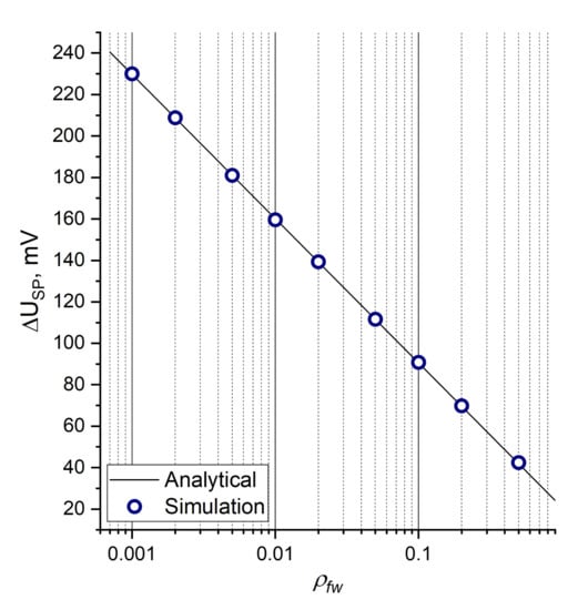
Figure 4.
Dependence of SP anomaly amplitude on formation water resistivity, obtained using the developed algorithm (circles) at reservoir thickness = 2.16 m ( = 20) and calculated (solid line) with the formula for static SP.
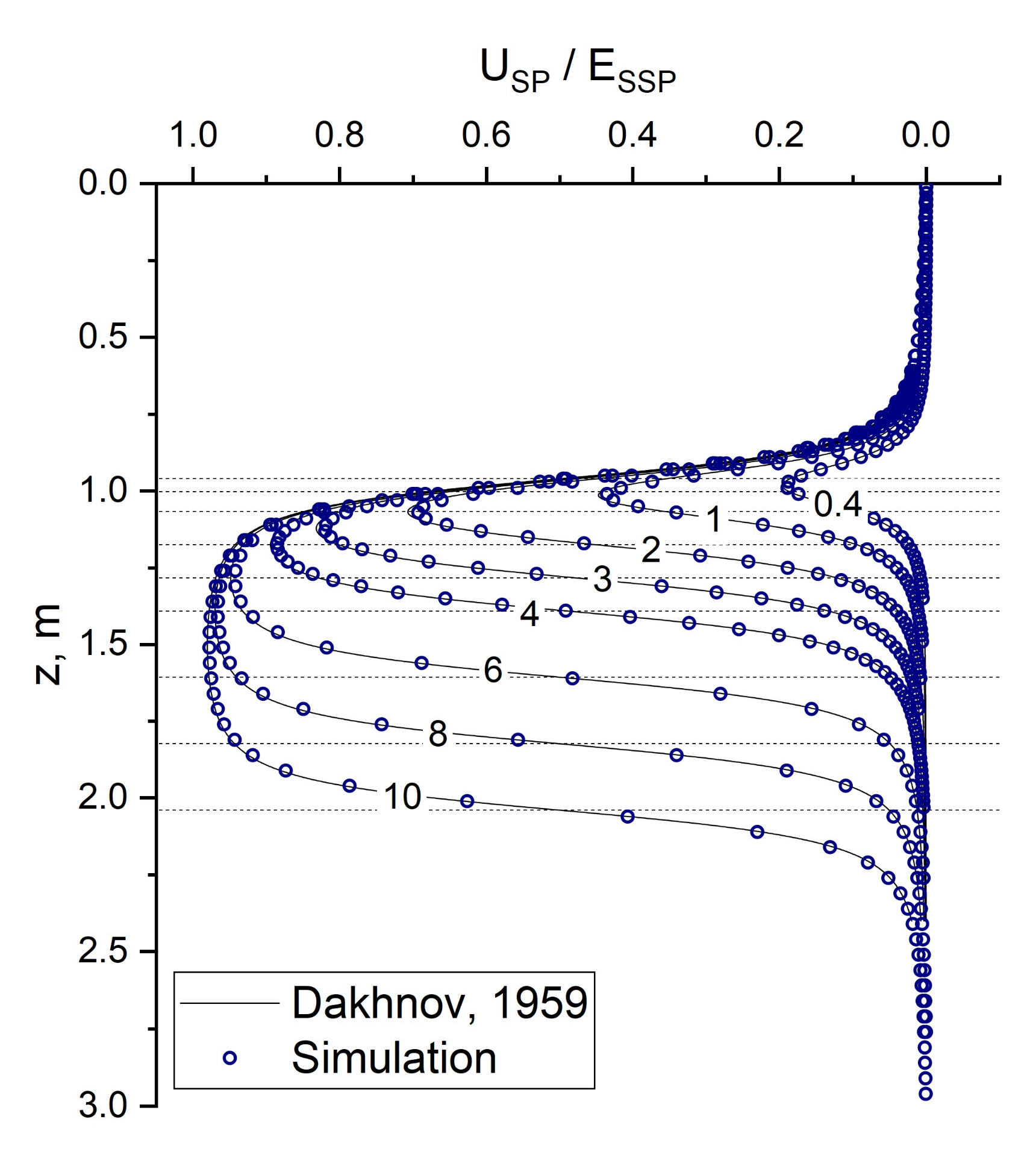
The influence of geometrical parameters on the magnitude and shape of the SP logging curve can be evaluated within the framework of the considered model. Simulation results were obtained for formations of different thickness and compared with the analytical formula given in [2] for the approximation of infinitely extended dipole layers (Figure 5). The effect of finite reservoir thickness manifests itself in a decrease in the observed amplitude of the SP anomaly relative to the static spontaneous potential .

Figure 5.
SP logging curves normalized to the static SP value from the thickness of the permeable formation. The cyphers of the corresponding curves denote the ratio of reservoir thickness to borehole radius. Circles are the results of calculation with the proposed numerical algorithm; the solid line is the calculation according to the analytical formula presented in [2].
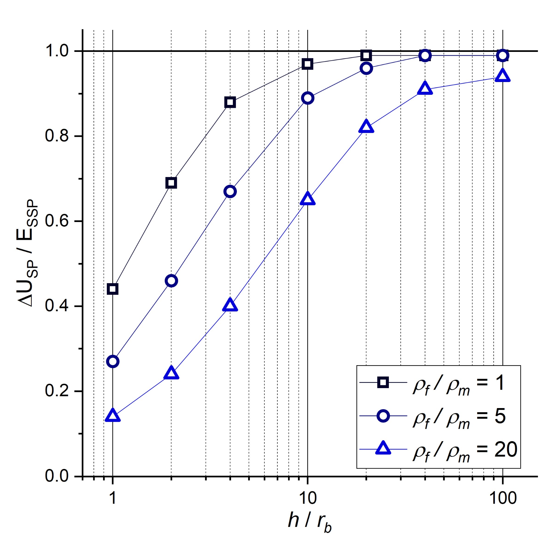
In general case, the ratio of the resistivities of both the permeable formation and the adjacent formations to the resistivity of the drilling mud can significantly affect the shape and amplitude of SP signals. Figure 6 shows the dependence of SP anomaly amplitude, normalized to the value of static SP, on the thickness of the sandstone reservoir for different ratios of reservoir and drilling mud resistivity. In this case, the resistivity of the adjacent formations is assumed to be equal to the resistivity of the reservoir. As can be seen from Figure 6, the greater the sandstone reservoir resistivity exceeds the mud resistivity, the greater the difference between the SP anomaly amplitude and the static SP at a given value of . The result is consistent with the correction charts for SP logging data [38].
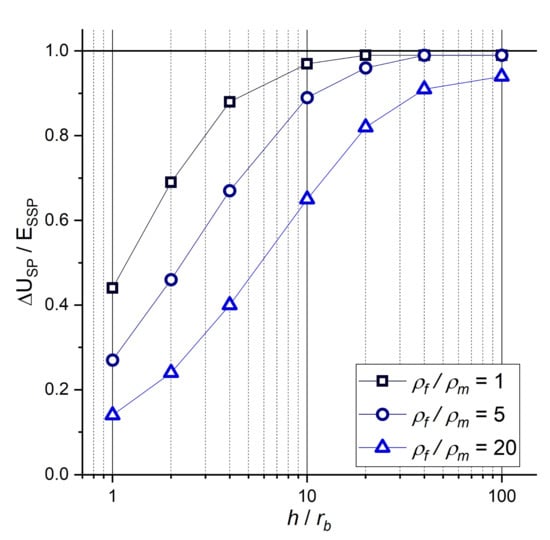
Figure 6.
Dependence of SP anomaly amplitude, normalized to the value of static SP, on the thickness of the permeable formation for different relationships between the resistivity of the sandstone formation and the drilling fluid.
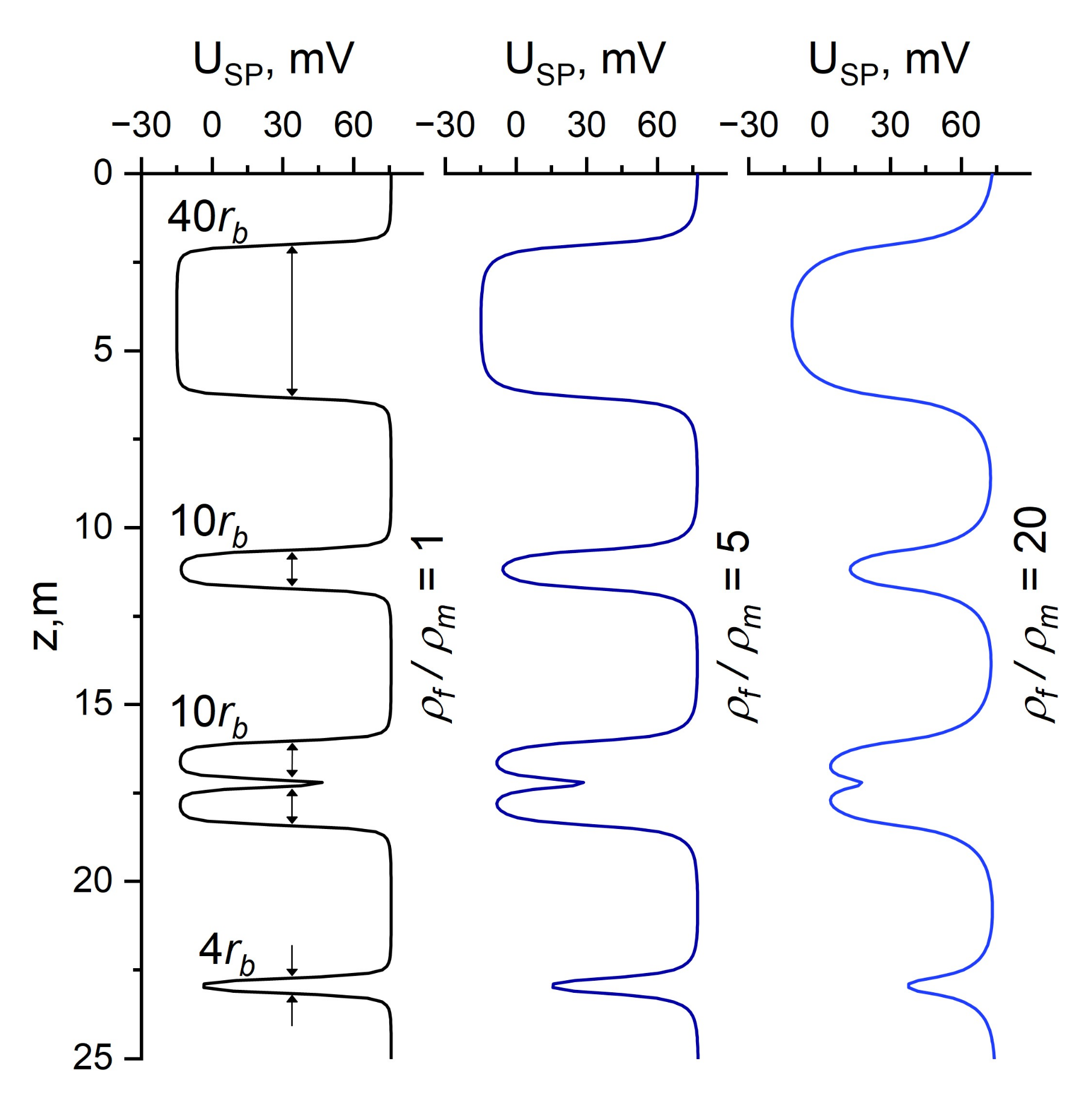
4.2. Numerical Modeling
The proposed algorithm is used to perform numerical simulations in typical model cases. First of all, we simulated a set of alternating sandstone beds of different thicknesses interlaid with shale sediments, for various ratios of the resistivity of the formation and the drilling fluid (Figure 7). The model was represented by sandstone layers of different thickness ( = 40; = 10; = 4), separated by clay interlayers of equal thickness ( = 2), and included a sandstone layer of 10, containing in the center a thin clay interlayer ( = 2). Modeling was performed for three cases with the ratio of the sandstone reservoir resistivity to the mud resistivity equal to 1, 5 and 20. In the intervals of thick reservoirs, the amplitudes of SP anomalies are close in value at different resistivity ratios. In this case, with decreasing reservoir thickness, a pronounced decrease in the amplitude, accompanied by smoothing of the SP signal diagram in the areas of intersection of reservoir boundaries with increasing permeability ratio of the reservoir and drilling fluid was observed. The amplitude of the SP anomaly of a sandstone reservoir containing a thin clay interlayer is less than the amplitude of the anomaly of a homogeneous reservoir of the same thickness. At the same time, the amplitude of the SP anomaly in the interbedded layer is greater than the amplitude of the anomalies in the constituent sandstone beds if they are separated by a thick clay interlayer.
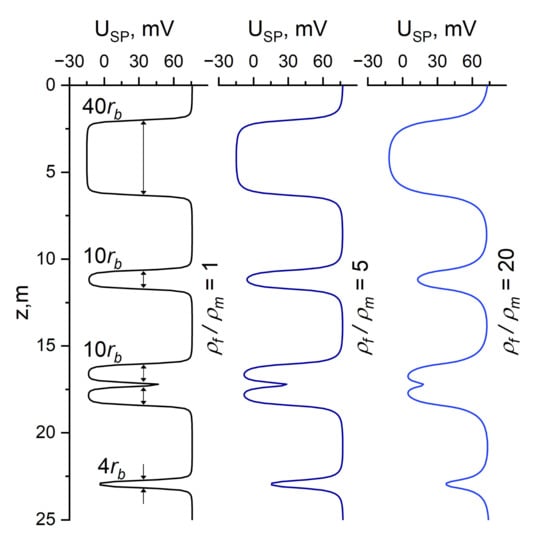
Figure 7.
SP log diagrams in a model of alternating sandstone beds of different thicknesses in shale sediments as a function of reservoir/mud resistivity ratio.
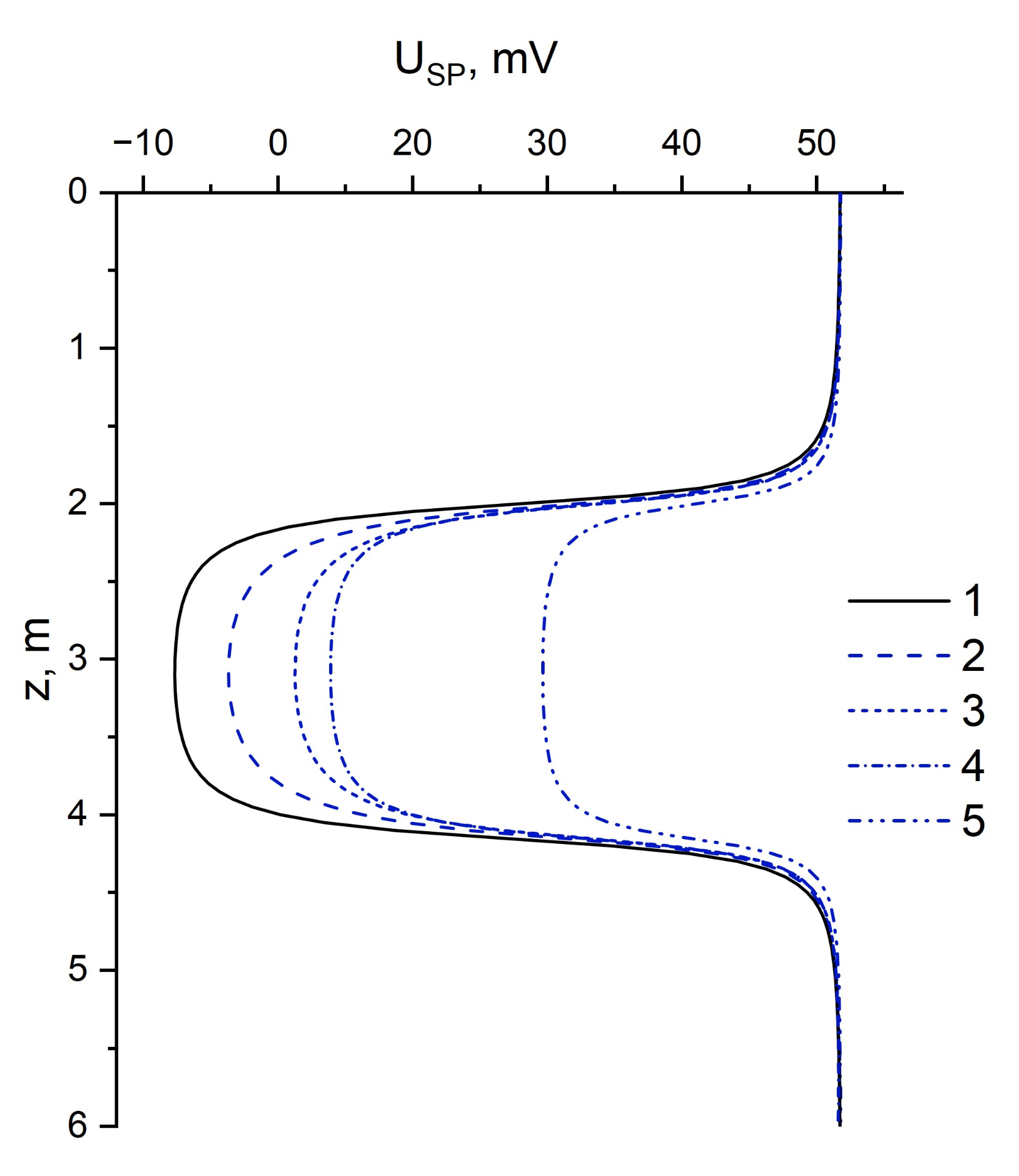
The above numerical experiments were performed without taking into account the clay content of the reservoir formation. In accordance with Section 2.2, simulation of SP logging data in the interval of reservoir formation characterized by both changes in clay content and its type (Figure 8) was carried out. The clay content was accounted for by calculating the average cation exchange capacity of the reservoir bed, using (9). The calculated cation exchange capacity determines the value of both diffusion–adsorption EMF coefficient of the reservoir, according to (6) and (7), and its resistivity (8). Kaolinite, illite and smectite are considered as clay minerals. Cation exchange capacities of these minerals and other modeling parameters are given in Table 2. Note that an increase in clay material content in the reservoir formation is accompanied by a change in porosity. It is seen that increasing the clay material content in the reservoir by 30% and decreasing the porosity by 5% relative to the case of pure sandstone leads to a more than twofold decrease in the amplitude of SP anomaly. At fixed values of clay material content and porosity, the amplitude of SP anomaly significantly decreases for sandstone reservoir with clay mineral having higher values of cation exchange capacity.
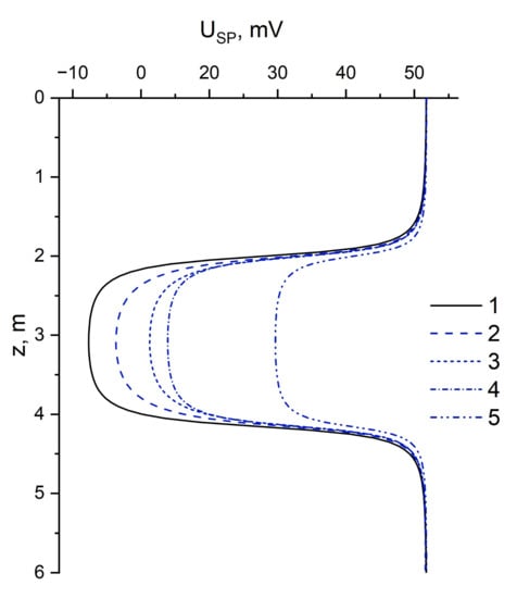
Figure 8.
Influence of clay material content and clay mineral type on the SP signal. Diagrams number (porosity/content of clay material and type of clay mineral): 1–20/0%; 2–15/30% kaolinite; 3–15/30% illite; 4–18/10% smectite; 5–15/30% smectite.
Table 2.
Parameters used in numerical simulation of SP logging curve, taking into account claystone reservoir.
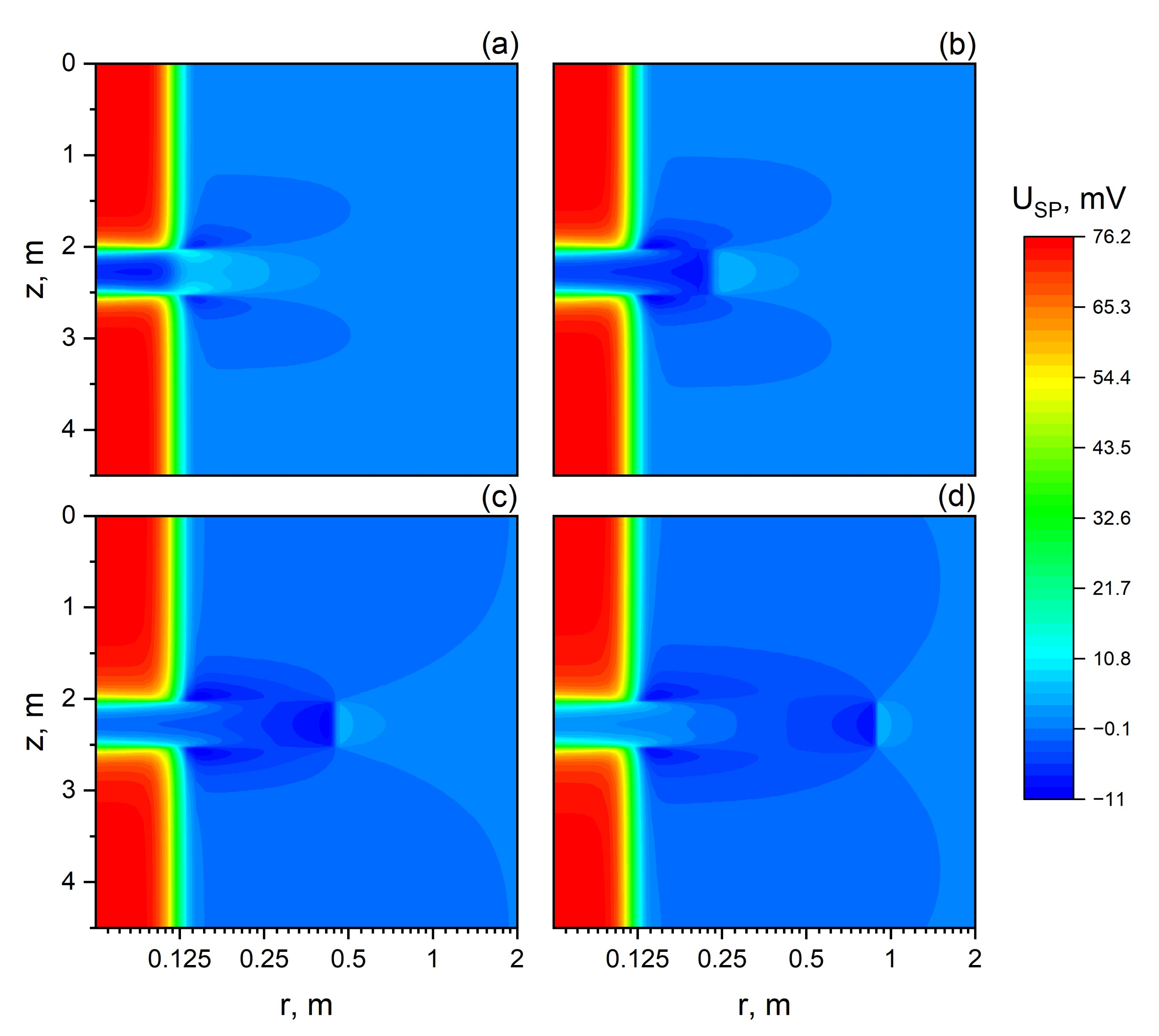
As described in Section 2.1, during the process of drilling the filtrate of freshwater clay mud penetrates into the permeable formation (Figure 1), which leads to a change in the radial profile of the resistivity, characterizing the depth of invasion and the value of change of resistivity of the formed zone of drilling mud filtrate invasion . The latter, according to (Schlumberger, 1989), can be considered equal to 75% of the drilling mud resistivity in the borehole (1.5 Ohm m). Two-dimensional potential distribution in the studied area was analyzed in the presence of the borehole, invasion zone and unchanged part of the permeable formation (Figure 9). Since the electrochemical source of SP is non-zero only in the area characterized by the salinity gradient, increasing the radius of the invasion zone of the mud filtrate is accompanied by a decrease in the amplitude of the SP anomaly.

Figure 9.
Distribution of SP in the studied area for different radii of the mud filtrate invasion zone in the permeable sandstone bed of 0.5 m thickness. Radius of invasion zone: 0.108 m (a); 0.216 m (b); 0.432 m (c) and 0.864 m (d).
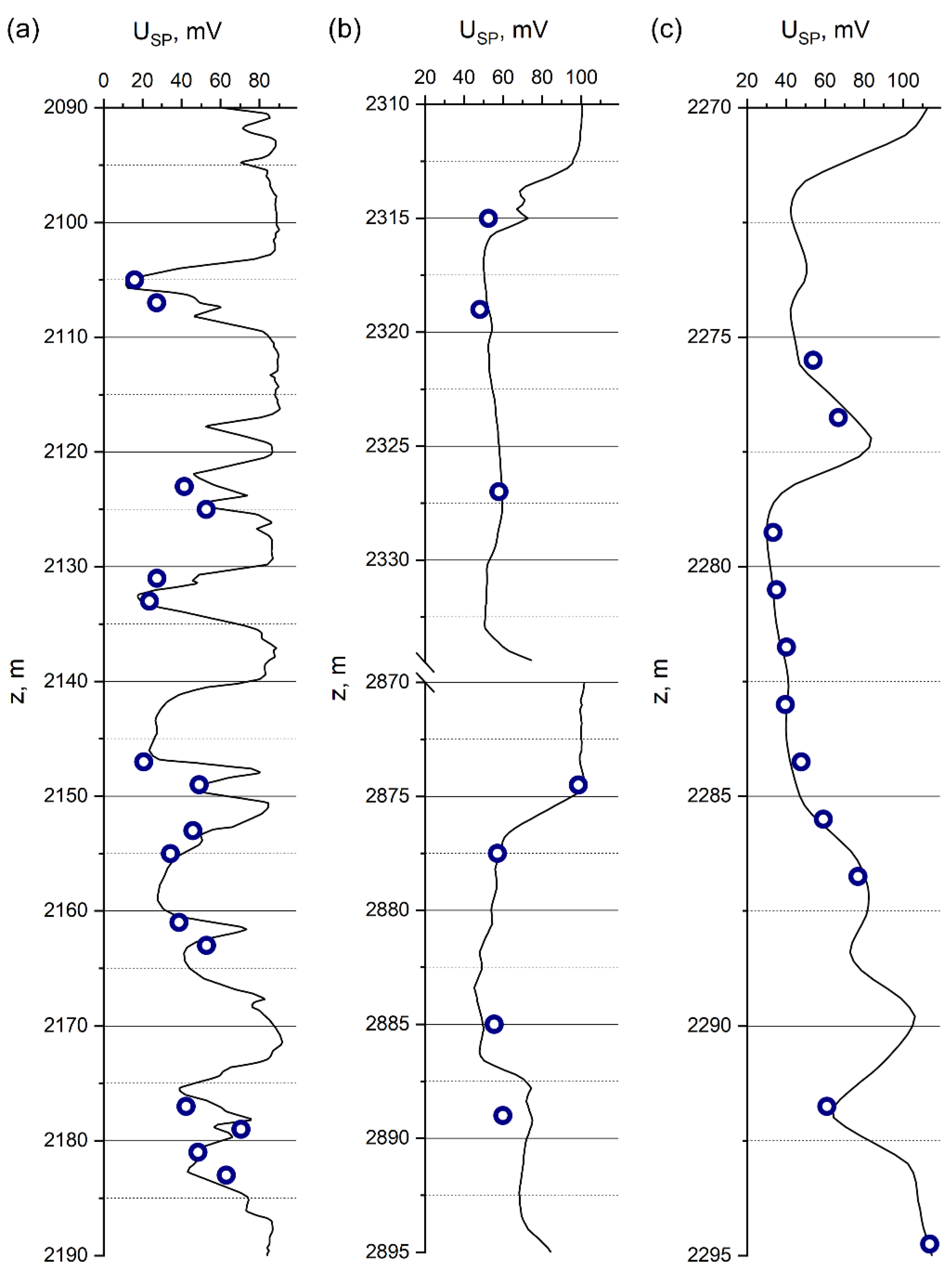
4.3. Comparative Analysis of Synthetic and Practical Data
Using the proposed algorithm, simulation and comparative analysis of synthetic and practical SP logging data were performed (Figure 10). To initialize the model parameters, data on the diffusion–adsorption activity of rocks obtained from laboratory studies of core samples from intervals of Cretaceous deposits uncovered by wells of a number of fields in the Latitudinal Ob Region of Western Siberia were used. Presented results include the simulation of SP logging data for the Lower Cretaceous AS10, BS9-BS13 and BS16-BS20 oil-bearing strata of the Achimov formation represented by irregularly interbedded sandstones and siltstones in shale sediments. In the presented interval of well A, the diffusion–adsorption activity of the sandstone is characterized by values from 0.75 to 26.7 mV and that of the siltstone by values from 16.5 to 31.1 mV. In the well B interval, this parameter has values: for sandstone from 6.3 to 21.3 mV, in the well C interval: from 3.65 to 41.7 mV and from 13.45 to 19.4 mV for sandstone and siltstone, respectively. Since these values of the diffusion–adsorption activity of rocks were measured under laboratory conditions at room temperature (25 °C), while at the considered depth intervals the temperature reaches about 75 °C, a temperature correction is taken into account. In this case, since is linearly dependent on temperature, its correct value can be determined by the formula: , where the factor .
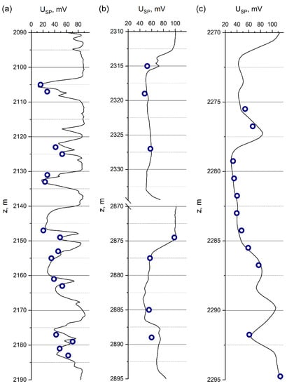
Figure 10.
Comparative analysis of synthetic (circles) and practical (line) SP logging data for different in-depth oil-bearing formations of the Lower Cretaceous deposits of the Achimov formation, penetrated by wells of the fields of Latitudinal Ob Region of Western Siberia. For well A layers BS9-BS13 are considered (a); for well B-AS10, BS16-BS20 (b), for well C-AS10 (c).
The results of numerical simulation of SP logging data using data on diffusion–adsorption activity of rocks obtained from laboratory core studies agree well with the practical data. Thus, the average value of relative discrepancy between synthetic and practical data is: well A—0.24, well B—0.11, well C—0.06.
5. Conclusions
We proposed a new computational algorithm for modeling SP logging data in the axial symmetry approximation based on the finite element method. The physical–mathematical statement of the SP problem was carried out using the coupled fluxes formalism, which allowed consideration of the effect of the electrochemical source of SP from the fundamental principles. The model of geological medium was presented, with the distribution of its electrophysical parameters approximated by sigmoidal functions that allowed simulation of SP signals for a wide range of parameters characterizing real experimental conditions. The developed algorithm was tested by the simulation of SP signals in the model of fluid-saturated sandstone to establish the characteristic effects, including the dependence of SP anomaly amplitude on formation water salinity, influence of permeable formation thickness and dependence of SP on the relationship between the reservoir and drilling fluid resistivity. The used physical–mathematical model allowed the simulation of SP signals in a clayey sandstone formation, as well as in the case of drilling mud filtrate invasion. The capabilities of the algorithm were demonstrated by a comparative analysis of synthetic and practical SP logging data, based on the results of laboratory studies of core from intervals of the Lower Cretaceous deposits exposed by wells in a number of Western Siberian fields.
The results obtained aim at the development of the SP method and allow us to formulate relevant directions for practical application. Since SP logging is performed in all wells and the data are widely available, including at the late stage of field development, it is extremely important to search for missed oil-bearing intervals. The solution of this problem becomes possible by reinterpretation of archival materials at a qualitatively new level with the use of modern software. One of the ways to increase informativity of the SP method while studying geological well sections is the use of oxidizers in drilling mud in order to contrast permeable intervals. For this purpose, it is necessary to use software–algorithmic tools, taking into account a full model description of physical and chemical processes, including redox, taking place both in a well and near-wellbore space. Another direction is the creation of realistic models of the geological environment to substantiate new geophysical methods of mineral exploration, including the method of pulsed electromagnetic sounding of the Bazhenov Formation with a system of highly deviated wells. All this is successfully facilitated by the active involvement of modern computational algorithms for solving forward and inverse SP problems in the class of multidimensional media models, including the one developed.
Author Contributions
Conceptualization, M.E.; methodology, M.E., A.G. and O.N.; investigation, A.G.; writing—original draft preparation, M.E., A.G. and O.N.; writing—review and editing, M.E., A.G. and O.N.; supervision, M.E.; project administration, M.E.; funding acquisition, M.E. All authors have read and agreed to the published version of the manuscript.
Funding
Research work related to the construction of realistic models of the Lower Cretaceous deposits based on SP data and using the developed computational algorithm was carried out with the financial support of the Russian Science Foundation, grant number 19-77-20130.
Data Availability Statement
The data presented in this study are available on request from the corresponding author.
Acknowledgments
The authors are grateful to the editors for offering to publish the article in this Special Issue.
Conflicts of Interest
The authors declare no conflict of interest.
References
- Doll, H.G. The S.P. Log: Theoretical Analysis and Principles of Interpretation. Trans. AIME 1949, 179, 146–185. [Google Scholar] [CrossRef]
- Dakhnov, V.N. Prospective Geophysics; Pershina, V.G., Fedotova, I.G., Eds.; State Scientific and Technical Publishing House of Oil and Mining and Fuel Literature: Moscow, Russia, 1959. (In Russian) [Google Scholar]
- Ellis, D.V.; Singer, J.M. Well Logging for Earth Scientists; Springer: Berlin/Heidelberg, Germany, 2007. [Google Scholar]
- Hunt, C.W.; Worthington, M.H. Borehole electrokinetic responses in fracture dominated hydraulically conductive zones. Geophys. Res. Lett. 2000, 27, 1315–1318. [Google Scholar]
- Minsley, B.J.; Sogade, J.; Morgan, F.D. Three-dimensional source inversion of self-potential data. J. Geophys. Res. Solid Earth 2007, 112, 1–13. [Google Scholar] [CrossRef] [Green Version]
- Revil, A.; Linde, N.; Cerepi, A.; Jougnot, D.; Matthäi, S.; Finsterle, S. Electrokinetic coupling in unsaturated porous media. J. Colloid Interface Sci. 2007, 313, 315–327. [Google Scholar] [CrossRef] [Green Version]
- Stoll, J.; Bigalke, J.; Grabner, E.W. Electrochemical modelling of self-potential anomalies. Surv. Geophys. 1995, 16, 107–120. [Google Scholar] [CrossRef]
- MacAllister, D.J.; Graham, M.T.; Vinogradov, J.; Butler, A.P.; Jackson, M.D. Characterizing the Self-Potential Response to Concentration Gradients in Heterogeneous Subsurface Environments. J. Geophys. Res. Solid Earth 2019, 124, 7918–7933. [Google Scholar] [CrossRef] [Green Version]
- Arora, T.; Linde, N.; Revil, A.; Castermant, J. Non-intrusive characterization of the redox potential of landfill leachate plumes from self-potential data. J. Contam. Hydrol. 2007, 92, 274–292. [Google Scholar] [CrossRef] [PubMed]
- Maineult, A.; Bernabé, Y.; Ackerer, P. Detection of advected, reacting redox fronts from self-potential measurements. J. Contam. Hydrol. 2006, 86, 32–52. [Google Scholar] [CrossRef] [PubMed]
- Wyllie, M.R.J. A quantitative analysis of the electrochemical component of the S. P. curve. Pet. Trans. AIME 1949, 1, 17–26. [Google Scholar] [CrossRef]
- Salazar, J.M.; Wang, G.L.; Torres-verdín, C.; Lee, H.J. Combined simulation and inversion of SP and resistivity logs for the estimation of connate-water resistivity and Archie’s cementation exponent. Geophysics 2008, 73, E107–E114. [Google Scholar] [CrossRef] [Green Version]
- Singha, D.K.; Rai, N.; Madhvi Maurya, M.; Shankar, U.; Chatterjee, R. Interpretation of Self-Potential (SP) Log and Depositional Environment in the Upper Assam Basin, India; Biswas, A., Ed.; Springer International Publishing: Cham, Switzerland, 2021; pp. 279–301. [Google Scholar] [CrossRef]
- Miah, M.I. Porosity assessment of gas reservoir using wireline log data: A case study of bokabil formation, Bangladesh. Procedia Eng. 2014, 90, 663–668. [Google Scholar] [CrossRef] [Green Version]
- Worthington, A.E.; Meldau, R.F. Departure Curves for the Self-Potential Log. Pet. Trans. AIME 1958, 213, 11–16. [Google Scholar] [CrossRef]
- Segesman, F. New SP correction charts. Geophysics 1962, 27, 815–828. [Google Scholar] [CrossRef]
- Revil, A. Ionic Diffusivity, Electrical Conductivity, Membrane and Thermoelectric Potentials in Colloids and Granular Porous Media: A Unified Model. J. Colloid Interface Sci. 1999, 212, 503–522. [Google Scholar] [CrossRef] [PubMed]
- Bautista-Anguiano, J.; Torres-Verdín, C.; Strobel, J. Mechanistic 3D finite-difference simulation of borehole spontaneous potential measurements. Geophysics 2020, 85, D105–D119. [Google Scholar] [CrossRef]
- Sill, W.R. Self-potential modeling from primary flows. Geophysics 1983, 48, 76–86. [Google Scholar] [CrossRef]
- Tatsien, L.; Yongji, T.; Yuejun, P. Mathematical model and method for spontaneous potential well-logging. Eur. J. Appl. Math. 1994, 5, 123–139. [Google Scholar] [CrossRef]
- Pan, K.J.; Tan, Y.J.; Hu, H.L. Mathematical model and numerical method for spontaneous potential log in heterogeneous formations. Appl. Math. Mech. 2009, 30, 209–219. [Google Scholar] [CrossRef]
- Dobroka, M.; Szabo, P.N. The inversion of well log data using simulated annealing method. Publ. Univ. Miskolc Ser. A Min. Geotechnol. 2001, 59, 115–138. [Google Scholar]
- Akimova, E.; Belousov, D. Parallel Algorithms for Solving Linear Systems with Block-Fivediagonal Matrices on Multi-Core CPU. CEUR Workshop Proc. 2016, 1729, 38–48. [Google Scholar]
- Akimova, E.N.; Belousov, D.V.; Misilov, V.E. Algorithms for solving inverse geophysical problems on parallel computing systems. Numer. Anal. Appl. 2013, 6, 98–110. [Google Scholar] [CrossRef] [Green Version]
- Hristenko, L.A.S. Transformation of SP observations for solving engineering-geological problems. Min. Inform. Analyt. Bull. 2012, 5, 169–173. [Google Scholar]
- Biswas, A. Inversion of Amplitude from the 2-D Analytic Signal of Self-Potential Anomalies. In Minerals; IntechOpen: London, UK, 2018. [Google Scholar] [CrossRef] [Green Version]
- Eppelbaum, L.V. Review of processing and interpretation of self-potential anomalies: Transfer of methodologies developed in magnetic prospecting. Geosciences 2021, 11, 194. [Google Scholar] [CrossRef]
- Akgün, M. Estimation of some bodies parameters from the self potential method using Hilbert transform. J. Balk. Geophys. Soc. 2001, 4, 29–44. [Google Scholar]
- Zhang, G.J.; Wang, G.L. A new approach to sp computation—vector potential approach. IEEE Trans. Geosci. Remote Sens. 1999, 37, 2092–2098. [Google Scholar] [CrossRef]
- Jardani, A.; Revil, A.; Santos, F.; Fauchard, C.; Dupont, J.P. Detection of preferential infiltration pathways in sinkholes using joint inversion of self-potential and EM-34 conductivity data. Geophys. Prospect. 2007, 55, 749–760. [Google Scholar] [CrossRef]
- Woodruff, W.F.; Revil, A.; Jardani, A.; Nummedal, D.; Cumella, S. Stochastic Bayesian inversion of borehole self-potential measurements. Geophys. J. Int. 2010, 183, 748–764. [Google Scholar] [CrossRef] [Green Version]
- Ferguson, C.K.; Klotz, J.A. Filtration from Mud during Drilling. J. Pet. Technol. 1954, 6, 30–43. [Google Scholar] [CrossRef]
- Li, H.; Fan, Y.R.; Hu, Y.Y.; Deng, S.G.; Sun, Q.T. Joint inversion of HDIL and SP with a five-parameter model for estimation of connate water resistivity. Acta Geophys. Sin. 2013, 56, 688–695. [Google Scholar] [CrossRef]
- Dakhnov, V.N. Interpretation of Logging Diagrams; Gosgeoltekhizdat: Moscow, Russia, 1941. (In Russian) [Google Scholar]
- Archie, G.E. The Electrical Resistivity Log as an Aid in Determining Some Reservoir Characteristics. Pet. Trans. AIME 1942, 146, 54–62. [Google Scholar] [CrossRef]
- Waxman, M.H.; Smits, L.J.M. Electrical conductivities in oil-bearing shaly sands. Soc. Pet. Eng. J. 1968, 8, 107–122. [Google Scholar] [CrossRef]
- Nechaev, O.V.; Glinskikh, V.N. Three-dimensional simulation and inversion of lateral logging sounding and lateral logging data in media with tilt of the main axes of the dielectric anisotropy tensor. Vestnik NSU 2018, 16, 127–139. [Google Scholar] [CrossRef]
- Schlumberger. Log Interpretation Principles/Application; Schlumberger Educational Services: Houston, TX, USA, 1989. [Google Scholar]

Publisher’s Note: MDPI stays neutral with regard to jurisdictional claims in published maps and institutional affiliations. |
© 2022 by the authors. Licensee MDPI, Basel, Switzerland. This article is an open access article distributed under the terms and conditions of the Creative Commons Attribution (CC BY) license (https://creativecommons.org/licenses/by/4.0/).