1. Introduction
Electromagnetic (EM) geophysical exploration focuses on determining the electrical conductivity distribution in the subsurface in depth ranges from a few meters to more than one kilometer, depending on the particular application. In these depth ranges, the electrical conductivity of rocks is primarily controlled by the amount of pore fluids, the pore interconnectivity, the presence of metallic conductors (i.e., metal ores) and the abundance of clay minerals (cf. [
1]). Therefore, electromagnetic exploration is employed to tackle a wide range of geological issues, including groundwater geophysics (e.g., [
2]), mineral exploration (e.g., [
3]) and imaging geological structures and fault zones in general.
All EM methods utilize the principles of electromagnetic induction by measuring the Earth’s electromagnetic response due to an incident time-varying EM field or an imprinted time-varying current. A great benefit of EM induction methods is that the magnetic field response can be measured in the air. Compared to ground-based surveys, airborne EM has the advantage that an excellent coverage of data can be achieved in a short amount of time. However, the operation of manned aircraft is costly and can only be realized by specialized companies or research institutes. In contrast, unmanned aerial vehicles (UAVs) are more affordable and easy to operate and thus may become a viable alternative or complement to manned airborne surveys.
In recent years, the semi-airborne EM method, introduced by [
4,
5], has gained renewed interest, owing to its capability to explore deeper targets compared to entirely airborne EM systems and due to its higher efficiency than land-based controlled-source EM. Semi-airborne EM utilizes powerful transmitters deployed on the ground and a passive airborne sensor platform that measures the induced magnetic field while traversing over the area of interest. Due to the separation of transmitter and receiver and the dependence on a land-based EM source, this procedure is referred to as the semi-airborne EM method. A variety of such approaches have been reported (cf. [
6]). In general, they deploy either loop sources as transmitters (e.g., [
7]) or grounded electric bipoles (e.g., [
8]), rely either on induction coils, fluxgate magnetometers, superconducting quantum interference devices (SQUIDs) or optically pumped magnetometers (OPMs), and they evaluate the data either in the time (e.g., [
9]) or frequency domain (e.g., [
10]). However, common to all approaches is that the transmitter and the receiver are separated and that the airborne system is a passive one.
The semi-airborne EM setup is ideally suited to be implemented on UAVs. Over the past decades, along with technical developments regarding brushless electric motors, sensors and microprocessors, the variety of multicopters increased enormously while their costs decreased significantly (cf. [
11]). Due to the small size of these vehicles, a high spatial survey granularity can be ensured with flexible flight speeds and altitudes for numerous geophysical applications (e.g., [
12,
13,
14]). Challenges such as restrictions on payload and flight duration remain but are now within limits that are reasonable for semi-airborne EM surveying.
This manuscript discusses the methods and results of a semi-airborne EM survey utilizing grounded electric bipoles as the transmitters and a 25 kg maximum-take-off-weight multicopter, conceptualized for EM applications ([
15]), towing a passive sensor system. The template for an unmanned survey system is the helicopter-based semi-airborne EM system developed as part of the Deep Electromagnetic Sounding for Mineral Exploration (DESMEX) project (cf. [
16]). We report data from a test survey near Münster (Germany), in a topographically flat area located within the Münsterland Basin. The survey area provided good conditions for operating an unmanned aircraft system (UAS) and a subsurface characterized by flat-lying sedimentary strata. This test area was chosen to evaluate an implementation of the semi-airborne EM method using a multicopter.
We evaluate the data in the frequency domain and determine transfer functions between the injected current amperage and the measured magnetic flux density (cf. [
16]). Transfer function estimates are inverted into a model of the electrical resistivity distribution (the reciprocal of conductivity). Data are validated against ground-based reference recordings, and the resistivity model is validated against an independent direct current (DC) sounding and a magnetotelluric (MT) sounding.
2. Methods
2.1. Survey Setup
The basis for the evaluation of a UAS for semi-airborne EM application is a test survey carried out near Münster (Germany) in March 2021. The study area is located within the Münsterland Cretaceous Basin, a sedimentary basin primarily composed of cretaceous marl, sandstone and mudstone sequences covering a carboniferous basement (cf. [
17]). Due to its geological setting and undisturbed stratigraphy, the region is well-suited to test the performance of a UAS and to validate acquired data.
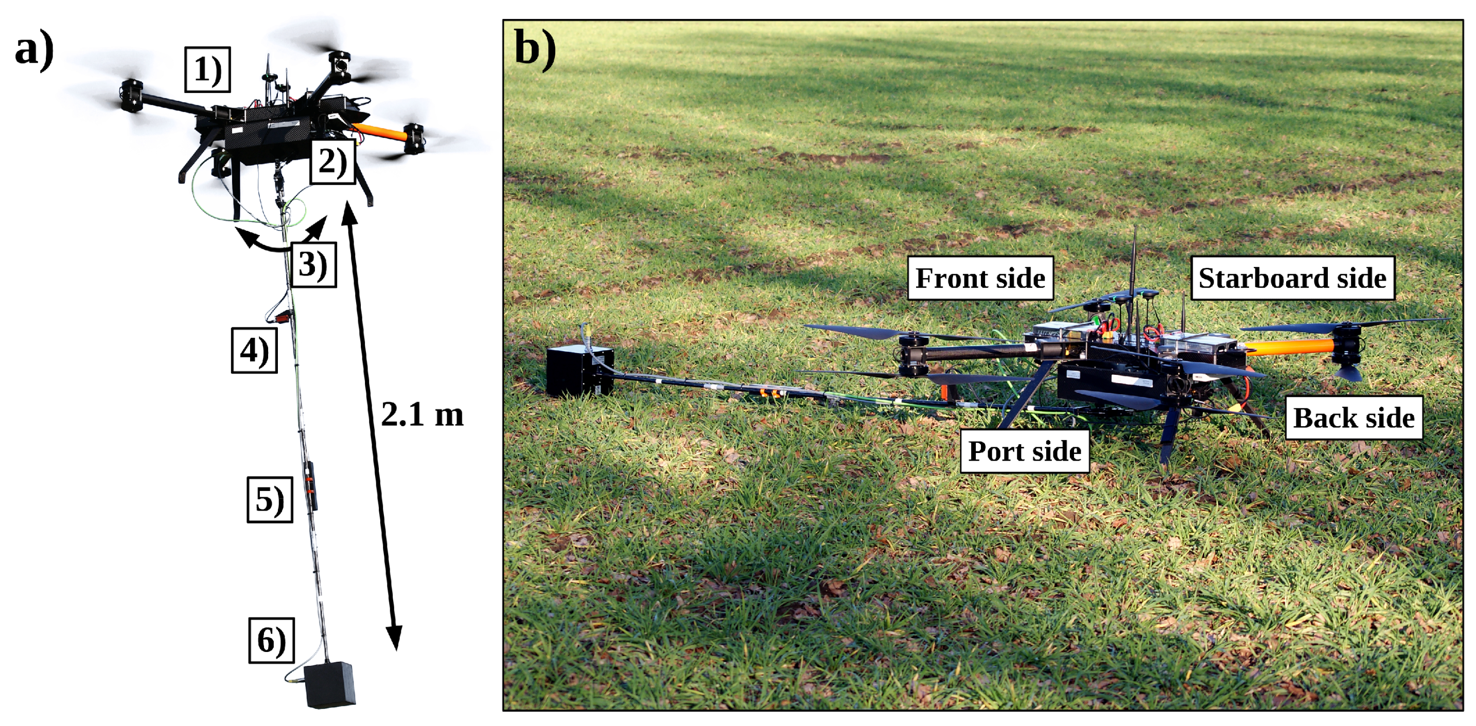
The utilized UAS was developed by Mobile Geophysical Technologies specifically for EM measurements and is based on an octocopter. This aircraft system is composed of a data logger rigidly mounted under the multicopter and magnetometers and an inertial measurement unit (IMU) suspended on a rigid rod (cf.
Figure 1). The rod, the logger housing, and the body parts of the UAV are made of carbon fiber to keep the takeoff weight low. There is a hinge on the bottom of the logger housing to which the rod is attached so that it can be tilted in the direction of flight. It is also possible to tilt the rod transversely, but this motion is limited by two separate damping elements placed on top of the rod. This design enables the UAV to take off in the forward direction while moving upward and land in the backward direction. The sensors are rigidly connected to the rod so that they are oriented opposite to the direction of flight after takeoff. A Metronix ADU-08e 24/32-Bit A/D unit was used for data logging and the mounted sensors are a Metronix SHFT-02e induction coil triple, a Bartington Mag-13MSL70 3-axis fluxgate sensor and a Xsens MTi-G-710 IMU. Sufficient power is provided by four 16,000 mAh lithium polymer batteries fastened in a recess within the body of the drone (UAS flight duration: ∼25 min). All mounted instruments are powered by a separate minor battery (5000 mAh, 11.1 V) attached to the drone body. In order to suppress UAV-related EM interferences (cf. [
18]) but still guarantee flight stability, the sensors were suspended up to a maximum distance of about 2 m from the vehicle.
In addition to the UAS, two ground stations were operated as ground references, equipped with a broadband (BB) coil triple (Metronix MFS-07e) and a high frequency (HF) coil triple (Metronix SHFT-02) and in each case equipped with an ADU-08e logger. Prior to the survey, a parallel test was carried out to cross-validate the ground and airborne HF sensors against the BB induction coils. Note that the SHFT-02 sensor was originally been designed for high-frequency recordings at frequencies greater than 1 kHz. To utilize this sensor also for lower frequencies in the scope of a semi-airborne EM setup, we calibrated them against the MFS-07e induction coils using recordings from the parallel test. We found that a calibration can be achieved down to frequencies as low as 10 Hz, but the sensitivity of the sensor becomes insufficient for our purpose at frequencies less than 30 Hz.
Within the survey area, four grounded horizontal electrical dipole (HED) transmitters were deployed, ranging between 800 m and 1.5 km in length. Steel spikes, steel lattices flatly embedded in the ground and iron rods drilled to a depth of up to 4 m were used to ground the poles. Contact resistances were in the order of 10
. The transmitters are displayed in
Figure 2. They were oriented mainly in east-west direction and were displaced in north-south direction by about 1 km each. We operated the transmitters using a Metronix TXM-22 power source with an integrated ADU-08e logger. A 100% duty cycle square wave current of up to 20 A was injected with a fundamental frequency of 32 Hz (cf.
Figure 3 and
Figure A1).
Each transmitter was operated and surveyed individually, with the completion of multiple flights per transmitter. The flight lines, with a spacing of about 150 m, are oriented mostly perpendicular to the HEDs. In total, 21 individual flight patches were realized, covering a total area of approximately 10 km. The UAS was flying at a constant velocity of 7 m/s at a flight altitude of 40 m above ground level. Both transmitter amperages and magnetic fields were measured at a sampling rate of 32,768 Hz. The sampling rate of the IMU, providing attitude angles, was 50 Hz.
2.2. Processing Workflow
The data processing workflow applied in this study is based mainly on the semi-airborne EM processing scheme described by [
16]. The primary objective of data processing is to determine transfer functions between the injection current
and the magnetic flux components
in the frequency domain from the linear relation
where
is a three-component magnetic transfer function at the point in space
and for the angular frequency
.
carries information about the electrical conductivity and constitutes data for further modeling and inversion.
The magnetic flux density is recorded in the body coordinate frame of the respective sensors. As a pre-processing step, it is required to rotate the data into earth-fixed coordinates. This was realized by using attitude angle recordings of the carried IMU (roll and pitch angles) and of the multicopter (yaw angle). Attitude angles of different origins were used as the multicopter provides a less drift-affected yaw output and the mounted sensors yield the same heading due to the non-torsion mounting. Data outliers were removed and the attitude angles interpolated to the sampling rate of the magnetometers. Removal of motion-induced voltages in the time domain, as discussed in detail in [
16], was not applied due to the low sampling rate and precision of the altitude data. However, it is anticipated that due to the moderate flying speed, vibrations are of minor importance, and motion-induced voltages, at least for the frequency bands of interest, are not a serious source of noise.
We transferred the time series for the current and the observed magnetic field into the frequency domain by performing a Short-Time Fourier Transform (STFT). This was executed for time windows having a length of 320 cycles of the fundamental period of the injected current, which corresponds to a window length of 10 s. A Hanning window function and a 50% overlap of the individual time windows were specified. Calibration functions were applied to the resulting spectral components. For further processing, discrete Fourier coefficients at the base frequency and at all odd harmonics were maintained. These spectral components were grouped into 15 logarithmically equidistantly distributed bins and a mean frequency was assigned to each bin. Besides spectral binning, the components of directly neighboring time windows were also included for regression.
The
i-th component of a transfer function
for a discrete frequency bin
b, at a centered position
and at a mean binned frequency
, is given by the least squares estimate
Here,
denotes the spectral components of the injected current amperage for the
b-th frequency bin and
denotes the spectral components of the observed magnetic field of the
i-th field component for the
b-th bin. The actual regression problem was solved using a least trimmed squares (LTS) estimator ([
19]).
The significance of estimation errors is small at low frequencies where regression is performed over only a few realizations (e.g., three for the lowest frequency). For the inversion, estimation errors alone are therefore insufficient to weight the data. Moreover, data weighting can be used to increase the importance of certain data subsets (e.g., low frequencies or large offsets). Here, we use a data weighting scheme considering the estimation error which is most significant, an absolute error on amplitude and phase (i.e., the assumed noise floor) and a relative amplitude error, which can also be transformed to a phase error. Regarding the amplitudes, an absolute error of 0.5 pT/A and a relative error of 10% were assumed. For the phase, an absolute error of was chosen.
3. Results
3.1. Spectral Analysis of Signal and Noise
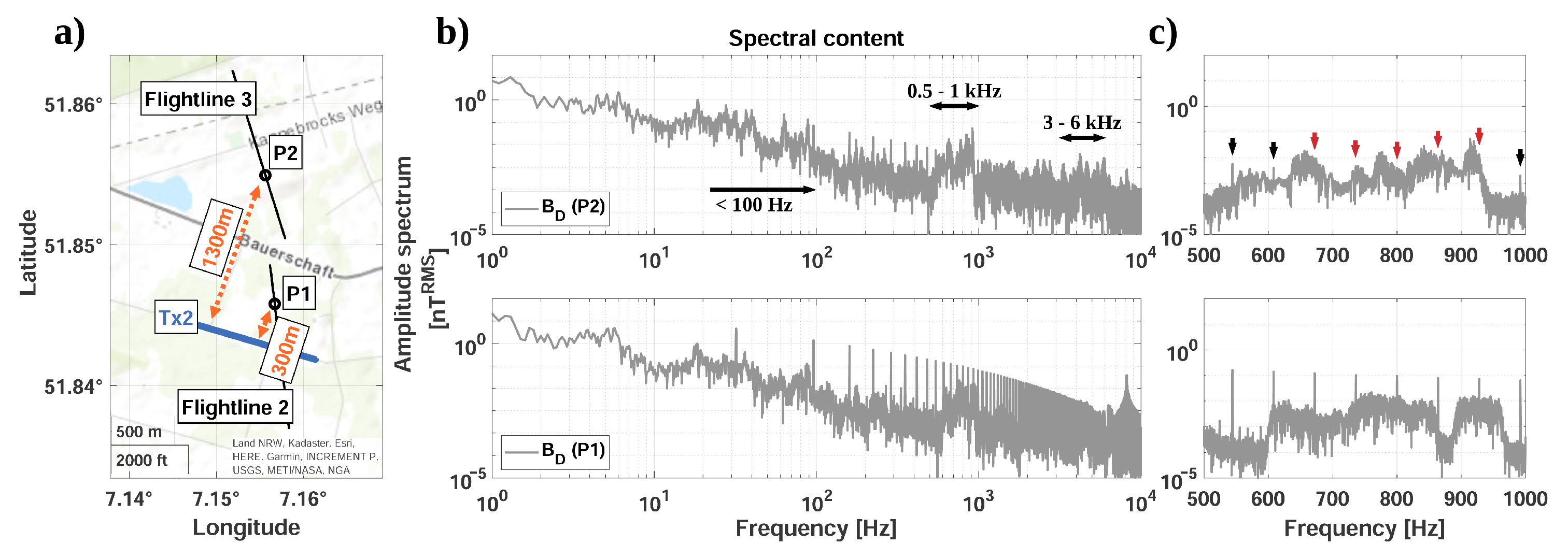
To evaluate the signal strength and noise level, we examine the spectral estimates of airborne data. In particular, we present amplitude spectra of the observed signal for short (300 m) and large offsets (1300 m) from the transmitter. Amplitude spectra of the downward component are depicted for both offsets in
Figure 4b,c. The map in
Figure 4a shows the position of the transmitter Tx2 and locations
and
where the spectra were estimated from an overflight. The spectra were determined following the procedure described in
Section 2.2.
For this measurement, we injected a square wave with a base period of 32 Hz (cf.
Figure 3a). The fundamental period and the associated odd harmonics can be clearly identified in the spectra of the airborne data (cf.
Figure 4). Note that the peak in the amplitude spectrum at about 8 kHz, caused by the transmitter pulse-width modulation, is also apparent. As expected, noise levels at both locations,
and
, are overall similar, but the signal decreases with increasing distance from the transmitter. The noise power increases towards the lower frequencies, reaching a similar order of magnitude as the signal at larger offsets (>1 km) for frequencies below 100 Hz.
The noise level is affected by distinct noise bands. Within the band ranging from 500 Hz to 1 kHz, a prominent noise plateau is observed (cf.
Figure 4c). Elevated noise plateaus are also observed at higher frequencies between 3 kHz and 6 kHz. These characteristics feature similar amplitude levels regardless of the measurement location and pose a problem to detect the signal at large offsets. At a distance of 300 m from the transmitter, the signal is clearly discernible at all harmonics, but this is no longer the case at a larger offset of 1300 m. For particular frequencies, moreover, the signal amplitude decreases below the ambient EM noise level.
The exact origin of these noise plateaus has not yet been investigated, but it is clear that they are related to the UAV and are not a local feature. Future improvements of the aircraft should aim at identifying and eventually optimizing the noise level in these frequency bands.
3.2. Hover Test
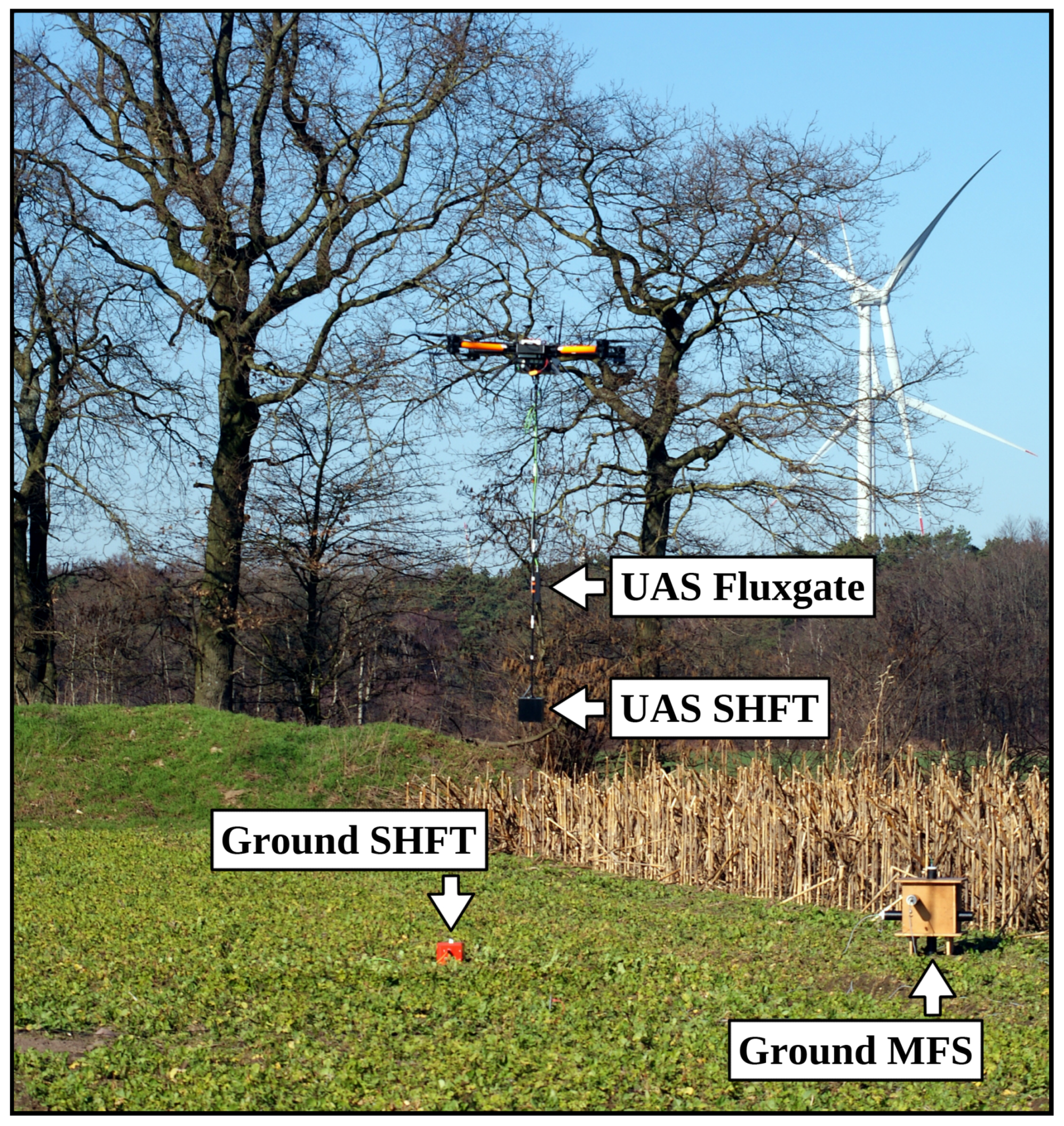
To test the reliability of the airborne recordings and the sensor functionality in general, we performed a hover test over a ground reference. For this purpose, two ground stations equipped with BB induction coils and a HF induction coil sensor, respectively, were operated and the UAS was hovering above them at low altitude (∼5 m) (
Figure A2). Both magnetometers attached to the multicopter were recording. Transmitter Tx1 was running for the hover test, and the ground stations were installed at a distance of 230 m to the transmitter. During hover, the multicopter attitude was varying and earth-fixed coordinates were calculated based on attitude recordings.
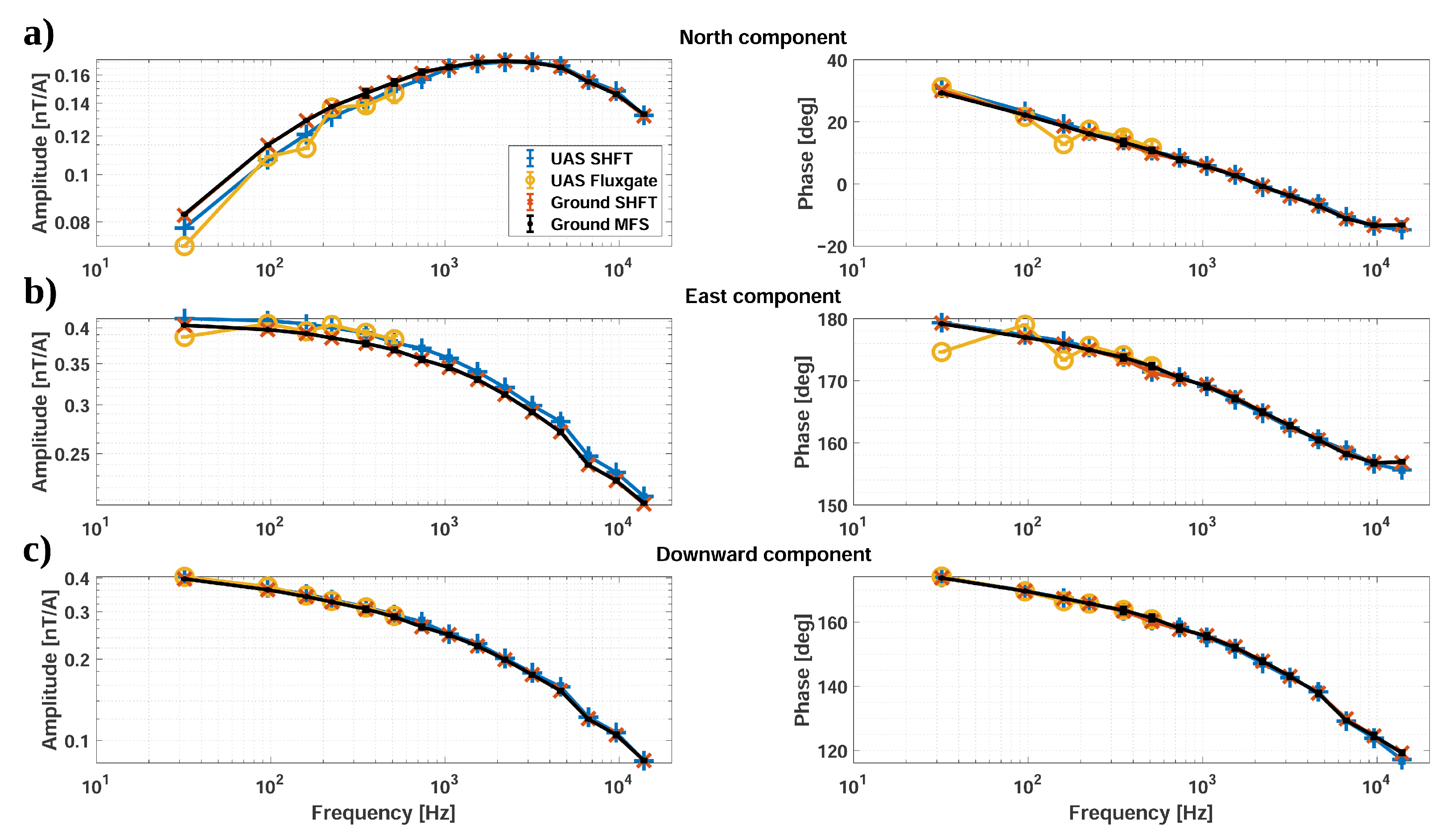
Figure 5 displays the frequency-dependent three-component transfer functions which we estimated based on the hover test for the four independent recordings, i.e., for two systems on the ground and the two sensors in air. All estimates are compatible. Both ground units exhibit a close to perfect match (the maximum phase offset is less than
) despite the different induction coil types being used. This suggests that the sensors are properly calibrated. Both UAS magnetometers also match very well, except for some scatter in the fluxgate estimates. This indicates that the airborne sensors are also correctly calibrated. We conjecture that the noisy estimates in the fluxgate data, especially for 32 Hz and 160 Hz, are due to motional noise, or due to the fact that the fluxgate sensor is suspended about 70 cm less than the HF sensor and thus is more susceptible to multicopter-related noise.
Airborne data exhibit an offset in amplitude (∼5%) relative to ground data, but the frequency-dependent characteristics are preserved. The phases between airborne and ground data are of good concordance over the entire period range. The reason for the amplitude offset is not entirely clear. Because the UAS was hovering, the difference in altitude or position could account for the discrepancy. However, it is more likely that a slight misorientation is responsible for the observed offset. Note that the north component of the transfer function determined from the airborne data is larger than that determined from the ground data, while the reverse applies for the east component. Hence, an attitude error, particular a systematic offset of the yaw angle estimate, could explain the differences.
Overall, we infer from the hover test that both the utilized UAS and the processing scheme are capable of determining semi-airborne EM transfer functions that are consistent with ground recordings.
3.3. Transfer Function Estimates
Transfer functions were determined for all airborne data using the processing scheme described in
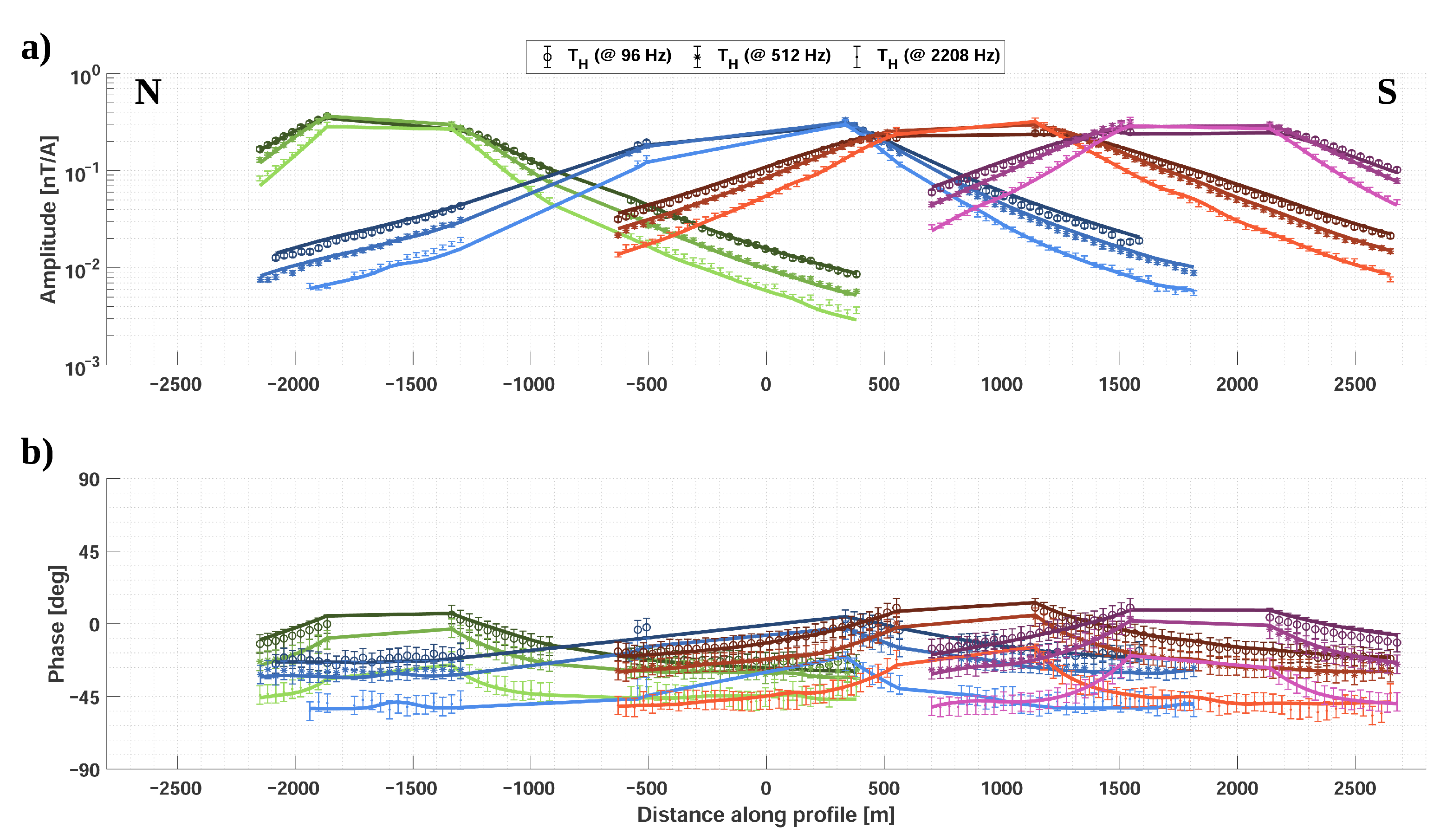
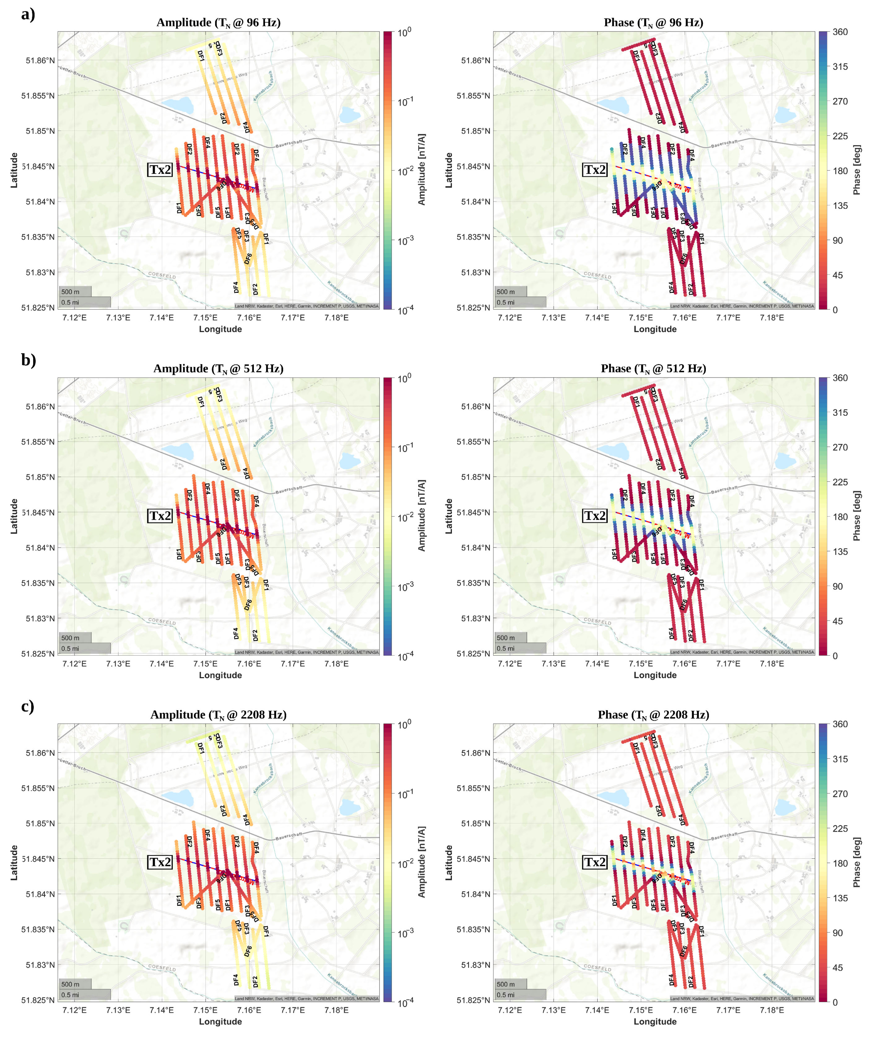
Section 2.2. In this section, we examine the quality and consistency of those estimates. As an example,
Figure 6b,c displays the north component of transfer functions along a profile across all four installed HED transmitters. The north component is the dominant horizontal component for transmitters oriented in the east-west direction. Data are shown as amplitude (
Figure 6b) and phase values (
Figure 6c) for the four associated transmitters and for three estimation frequencies: 96 Hz, 512 Hz and 2208 Hz. In
Figure A3 and
Figure A4, transfer function estimates for both north and downward component at individual frequencies are mapped.
Data depicted in
Figure 6b,c originate from individual flight lines of independent flights and have been concatenated to obtain a continuous profile line (cf.
Figure 6a). The profile line is oblique by
from the north direction. Only one transmitter was in operation at a time, but flight patches were designed to overlap in space. In the central part of the concatenated profile, between −700 m and 1700 m, observations from three independent transmitter signals are available. Outside of this central region of the profile, observations from two independent transmitters are available. A gap in the data at −800 m is due to a road which was not overflown. The processing shows that high-quality semi-airborne EM responses can be achieved with the UAS over a broad frequency range and distances of up to 2 km from the transmitter. As discussed in
Section 3.1, noise bands are observed between 0.5–1 kHz and 3–6 kHz. Transfer functions that fall within these bands are more distorted at larger offsets (not shown).
3.4. 2D Inversion of Multicopter-Based Data
In controlled source EM (including semi-airborne EM), transfer function estimates reflect the measurement geometry but they also carry information about subsurface electrical conductivity. Both the spatial decay of signals and their frequency dependency are influenced by EM induction processes in the subsurface. Inductive effects become more pronounced with increasing distance and increasing frequency, and penetration of induced currents (and thus the penetration depth of the method) increases with increasing distance and decreasing frequency. Hence, the sensitivity of controlled source EM transfer functions with respect to the lateral and vertical conductivity distribution is inhomogeneous and inverting data obtained from a single transmitter geometry can result in a geometrically biased resolution pattern. Two-dimensional inversion using multiple transmitters and overlapping line segments helps to recover subsurface structures with reduced bias due to the particular transmitter-receiver geometry.
Here, we use the MARE2DEM ([
20]) 2D controlled source EM inversion code, which is widely applied for marine and land-based data. The inversion code allows the placement of receivers in the air and is therefore also suitable to invert semi-airborne EM data. Previous applications of MARE2DEM to semi-airborne EM data are described in [
8,
21], where helicopter-based semi-airborne electromagnetic data acquired in the DESMEX project were treated, both in the frequency and time domain, respectively.
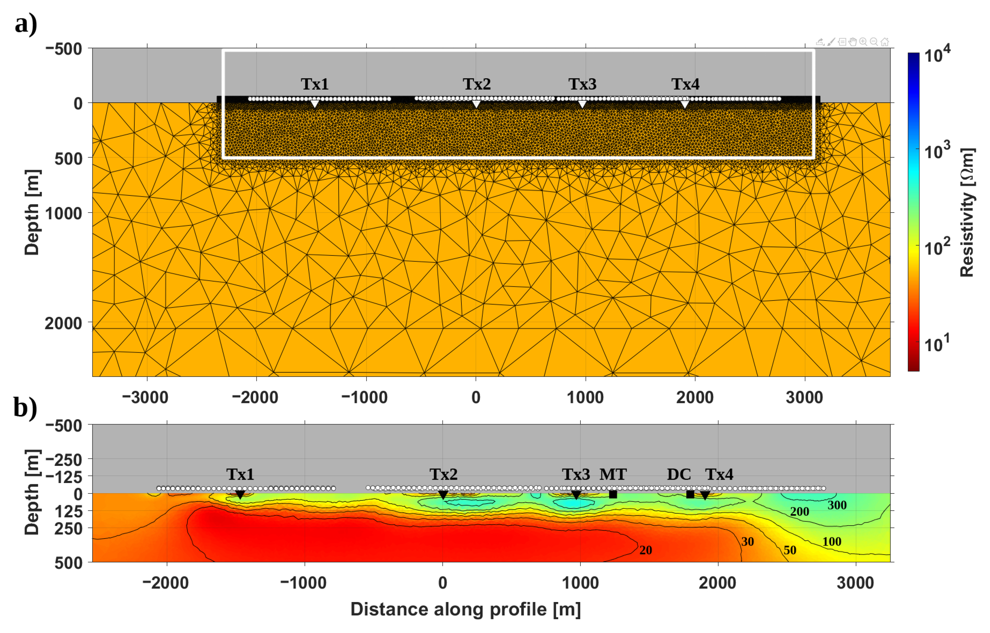
MARE2DEM uses an adaptive finite element algorithm to numerically compute the EM field at the receiver locations. The model can be generated from triangles with user-defined dimensions. In this application, we ensure a high near-surface model resolution by defining a parameterization with triangles with a side-length of 16 m, which is successively increased towards the model edges and the depth. A 200 × 200 km
homogeneous half-space bounding box with a resistivity of 50
m was chosen as the initial model. In
Figure 7a the model parameterization is depicted.
The finite element mesh employed to compute the model responses has at least the resolution of the model, but it is adaptively refined to meet numerical accuracy criteria (cf. [
20]). An Occam-type inversion strategy is applied, i.e., the model parameters are regularized to vary smoothly in space while achieving a predefined target misfit (cf. [
22,
23]). Once the chosen target misfit has been achieved, the inversion enters into a second phase, which aims at determining the smoothest model while keeping the target misfit. The target misfit is an error-weighted global measure of data misfit (cf. [
24]) and thus intimately related to the weighting imposed on the data. Tests were carried out to find a meaningful data weighting scheme and to define an appropriate target misfit. With the errors as defined in
Section 2.2, we found that a target misfit of 1.50 yields good results.
We jointly inverted the base-ten logarithm of the amplitude and the phase of the profile-parallel and downward component of magnetic transfer functions. Included were transfer functions for all transmitters and for 15 estimation frequencies between 32 Hz and 13,856 Hz. Only data points with a distance of more than 250 m and less than 2 km from the active source were included for inversion. This was done to avoid source-point inaccuracies for receivers close to the transmitter and to exclude data with a poor signal-to-noise ratio. Poor quality estimates were also masked manually. In particular, this was the case for data at greater distances and at frequencies within the UAV noise plateaus.
The inversion converged from a starting RMS of 4.64 to the chosen target misfit of 1.50 in 8 iterations.
Figure A5 and
Figure A6 depict observed data and predicted responses of the final inversion model. Only estimates used for inversion at three distinct frequencies are displayed. Note that missing estimates are due to data exclusion and individual masking. However, an excellent match of estimates and responses was achieved, showing a better match for the horizontal component (cf.
Figure A5) than for the vertical component (cf.
Figure A6). A reason for this could be the higher reliability of the horizontal over the vertical component due to the better signal-to-noise ratio (cf.
Figure A3 and
Figure A4). For a HED source, the horizontal component of the induced field becomes more dominant than the vertical component at large offsets from the transmitter. At higher frequencies the predicted response shows greater variability than actually observed. Noticeable is this prediction error in the downward component (cf.
Figure A6) at 2208 Hz for transmitter Tx3 at −100 m and at 1700 m profile distance and for transmitter Tx4 at 700 m profile distance.
In
Figure 7b the final inversion model is shown. The model is essentially composed of two layers. The near-surface layer has a resistivity between 100
m and 400
m and is slightly tilted to the south, from about 100 m thickness to 250 m thickness. A homogeneous resistivity in the range of 20–50
m is exhibited in the bottom layer. From the available data, the bottom depth of this conductor can not be identified. The pronounced stratification boundary is not continuous across the entire profile, dissolving at the profile margins. Here, the subsurface is characterized by resistive structures (unequal in size and resistivity) located directly beneath the northern and southern profile ends. Moreover, some lateral variation of resistivity is observed within the top layer, including more resistive bodies beneath transmitter Tx2 and Tx3. Each transmitter also seems to be embedded into a very shallow conductive patch with thicknesses of about 10 m. All these features show a clear dependence on the transmitter-receiver geometry and thus their geological validity might be doubted. Inferior data coverage above these domains may cause the appearance of these features in the model. It is also very likely that the shallow small-scale conductive patches are model artifacts, possibly a result of the uniformly recurring receiver spacing and insufficient coverage. In any case, these features should be omitted from any geological interpretation.
3.5. Model Validation
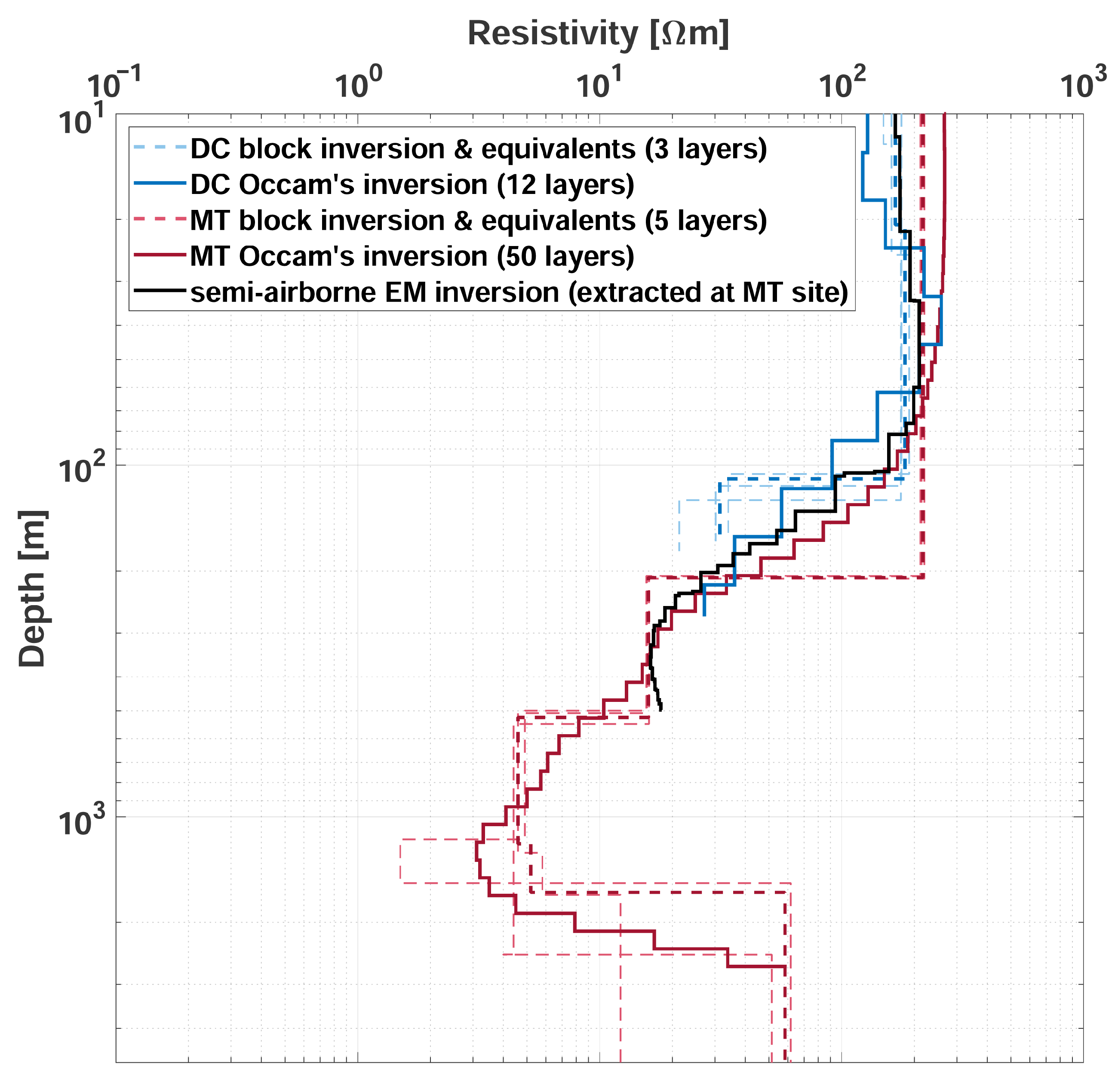
The inversion result based on the airborne recordings can be compared with results from other independent methods. In
Figure 8 1D inversion results based on data from a DC and a MT sounding carried out within the survey area are shown. The DC sounding was realized as a Schlumberger configuration along a road close to transmitter Tx4. To reduce influences from power lines and fences, the MT site was set up slightly offside on an open field close to the western margin of transmitter Tx3. There is a distance of about 1.5 km between the the DC sounding midpoint and the MT site. The MT soundings exhibit good data quality in the frequency range from 1 Hz to 1 kHz. A 1D interpretation could be justified from the similarity of the
and
elements of the estimated impedance tensor. We chose the
component for the inversion. Inversions were computed employing the IX1D software ([
25]) for both DC and MT soundings, using a homogeneous 100
m half-space as the initial model. An Occam-type inversion and block inversions models were computed.
When comparing the 1D models with the results from the 2D inversion of the semi-airborne data (cf.
Figure 8), high consistency of the subsurface conductivity of all three independent models is observed. All models reveal a resistive layer (>100
m) within the upper 100 m and a decrease in resistivity for the deeper formations. A minimum of 3–5
m is reached at depths greater than 400 m. Although the models match very well, there are minor differences indicating a shallower transition depth (cf. DC results) compared to a slightly deeper conductor (cf. MT results). However, the model based on semi-airborne EM data fits well between the other two results.
The applied methods exhibit different penetration depths depending primarily on electrode spacing (DC sounding), on excitation frequencies (semi-airborne EM), on the underlying resistor-conductor regime, on measurement duration at one location, and on achieved data quality. This fact leads to the differences in depicted model depths, where we obtain no reasonable information below 250 m for the DC result, below 500 m for the semi-airborne EM model and below 5 km for the MT model. Nevertheless, the MT results indicate another transition at a depth of around 2 km where the resistivity increases from less than 10 m to about 60 m.
4. Discussion
It has been found that magnetic transfer functions derived from multicopter-based semi-airborne EM recordings are consistent with co-located ground data and yield a high quality over a broad frequency-distance range (32 Hz–14 kHz, and up to 2 km, respectively). Applying a 2D inversion scheme, the data from both vertical and horizontal components along a concatenated profile, composed of overlapping segments from multiple flights across four independent transmitters, could be well fitted, suggesting that the line segments and the respective components are coherent.
Limitations on semi-airborne EM data quality results are primarily due to EM emissions from the multicopter and also the result of the limited accuracy of attitude recordings. Judging from the acquired airborne data, the noise level of the induction coils and the fluxgate sensor (at low frequencies) did not affect data in the frequency range of investigation. However, it is also clear that the employed HF induction coil triple is unsuited for obtaining precise recordings at frequencies below 30 Hz. Hence, the transmitter signal selected in this study (32 Hz fundamental frequency) represents a lower limit for our configuration.
One source of error in the semi-airborne EM data arises from inaccuracies by re-orientating body-frame coordinates into the earth-fixed system. As a result, a projection error will be encountered. Here, we used a self-contained IMU attached to the sensor rod to monitor the sensor attitude, but we observed a substantial drift of the yaw angle output. Such sensors have an inherent drift, in particular for the heading estimate, which accumulates over time and can lead to several degrees offset. We minimized that error by merging attitude data from IMU records and multicopter navigation logs. In this way, heading drift errors could be reduced but may remain significant. To further improve the accuracy of recorded attitude data, a more sophisticated IMU would need to be purchased.
At frequencies below 100 Hz, motional noise due to sensor motion within the external geomagnetic field seems to be a crucial source of error. This type of noise occurs in induction coils whenever the coil axes tilt with respect to the external field direction. Motional noise is one of the major sources of noise in airborne EM measurements. Due to the moderate flying speed, high-frequency vibrations are apparently not excited and interference of motion noise and signal is therefore restricted to the lowermost frequencies considered in this study.
At frequency bands between 0.5–1 kHz and 3–6 kHz, aircraft-related EM emissions are particularly severe and affect data quality. The noise level in these bands depends on the considered field component and also on flight maneuvers of the UAS. A straightforward approach to minimize these noise effects is to extend the sensor suspension. For this survey, the induction coil was suspended 2.1 m from the multicopter. Following the survey, test flights suggest that suspensions of 4 m can be realized without impairing flight stability, but there is a clear trade-off between suspension and flight safety.
Finally, the estimated resistivity model was found to be compatible with the regional geology. A distinct resistivity contrast, dipping from 100 m to 250 m depth along the profile, was found to explain the data, consistent with other observations and independent local 1D soundings. Due to limited electrode spacing of the performed DC sounding, we do not obtain information from depths below 250 m, whereas the MT sounding results, yielding a greater sensitivity towards deep-seated structures, indicate another resistivity interface. However, the results of the semi-airborne EM method do not clearly point towards this transition for the chosen excitation frequency, because the intermediate well-conducting layer effectively reduces the depth of investigation of this method.
5. Conclusions
In the framework of this study, a UAS-based semi-airborne EM survey covering an area of about 10 km was carried out and the acquired data were processed leading to an estimation of the subsurface conductivity distribution. The applied methodology, developed for helicopter-towed platforms, could be transferred for the most part to a unmanned system, the suitability of which was to be investigated in this study.
In order to evaluate the capability of a UAS for semi-airborne EM application, we have determined magnetic transfer functions for the entire survey area at frequencies ranging from about 32 Hz to 14 kHz, and used these as the basis for the calculation of 2D inversion models. We succeeded in ensuring good quality transfer function estimates up to a distance of 2 km from the deployed HED transmitters with high consistency and in estimating a conductivity model that matches the regional geology. Furthermore, the estimated model was validated with independent DC and MT measurements.
An important part of the study was the specification of application bounds for the demonstrated method. Limitations could be specified, and were found to be primarily the noise affected frequency bands between 0.5–1 kHz and 3–6 kHz, caused by the aircraft itself, and an increased noise level below 100 Hz, caused by motional noise effects. Future improvements will focus on reducing EM noise, which can be achieved by extending the sensor suspension, and on increasing the attitude data accuracy of the mounted sensors contributing significantly to the final data quality.
Although a UAS with its highly restricted load capacity and flight duration is impractical for techniques with a mounted high-power EM transmitter, these disadvantages become less significant in the case of transmitters deployed on the ground. Such a UAS-based approach has benefits over manned systems because of its agility, and surpasses the efficiency of ground-based methods.
Author Contributions
Conceptualization, P.O.K., M.B. and A.T.; methodology, M.B.; software, P.O.K., M.B. and A.T.; validation, P.O.K., M.B. and A.T.; formal analysis, P.O.K.; investigation, P.O.K., M.B., A.T., V.S., J.S., S.U. and S.K.; resources, M.B., V.S., J.S., S.U. and S.K.; data curation, P.O.K., M.B., V.S., S.U. and S.K.; writing—original draft preparation, P.O.K., M.B. and A.T.; writing—review and editing, P.O.K., M.B., A.T., V.S. and S.U.; visualization, P.O.K., M.B. and A.T.; supervision, M.B.; project administration, M.B.; funding acquisition, M.B. All authors have read and agreed to the published version of the manuscript.
Funding
This research has been funded by the Federal Ministry of Education and Research of Germany in the framework of DESMEX II (project no. 003R130AN). Parts of the instrumentation were funded by the German Research association (DFG) under grant INST 211/864-1 FUGG.
Institutional Review Board Statement
Not applicable.
Informed Consent Statement
Not applicable.
Data Availability Statement
Research data related to this study may be requested from the author. The consent of all associated project partners is required for data release.
Acknowledgments
We are grateful to the DESMEX working group members for valuable discussion on the method of semi-airborne EM and on multicopter implementation. The support of local landowners in the survey region was highly appreciated. We owe further thanks to Matthew J. Comeau, who helped to improve the readability of the manuscript.
Conflicts of Interest
The authors declare no conflict of interest. The funders had no role in the design of the study; in the collection, analyses, or interpretation of data; in the writing of the manuscript, or in the decision to publish the results.
Abbreviations
In this manuscript, the following abbreviations are used:
| BB | Broadband |
| DC | Direct current |
| DESMEX | Deep Electromagnetic Sounding for Mineral Exploration |
| EM | Electromagnetic(s) |
| HED | horizontal electric dipole |
| HF | High frequency |
| IMU | Inertial measurement unit |
| LTS | Least trimmed squares |
| MT | Magnetotelluric(s) |
| OPM | Optically pumped magnetometer |
| RMS | Root mean square |
| SQUID | superconducting quantum interference device |
| STFT | Short-Time Fourier Transform |
| UAV | Unmanned aerial vehicle |
| UAS | Unmanned aircraft system |
Appendix A
Figure A1.
Overview of all employed HED transmitters (Tx1: green, Tx2: blue, Tx3: red, Tx4: purple). (a): Time series section of the injected current amperage for each transmitter. (b): Stacked amplitude spectra of the respective transmitters. (c): Enlarged spectra between 500 Hz and 1 kHz.
Figure A1.
Overview of all employed HED transmitters (Tx1: green, Tx2: blue, Tx3: red, Tx4: purple). (a): Time series section of the injected current amperage for each transmitter. (b): Stacked amplitude spectra of the respective transmitters. (c): Enlarged spectra between 500 Hz and 1 kHz.
Figure A2.
Image of a hover test performed during the survey. Four magnetometers were involved: a Metronix SHFT-02 induction coil triple placed on the ground (Ground SHFT), a Metronix MFS-07e coil triple placed on the ground (Ground MFS), a Metronix SHFT-02e induction coil triple as part of the UAS (UAS SHFT) and a Bartington Mag-13MSL703-axis fluxgate sensor as part of the UAS (UAS Fluxgate). The heading of the UAV and its altitude (3–6 m) varied during hover.
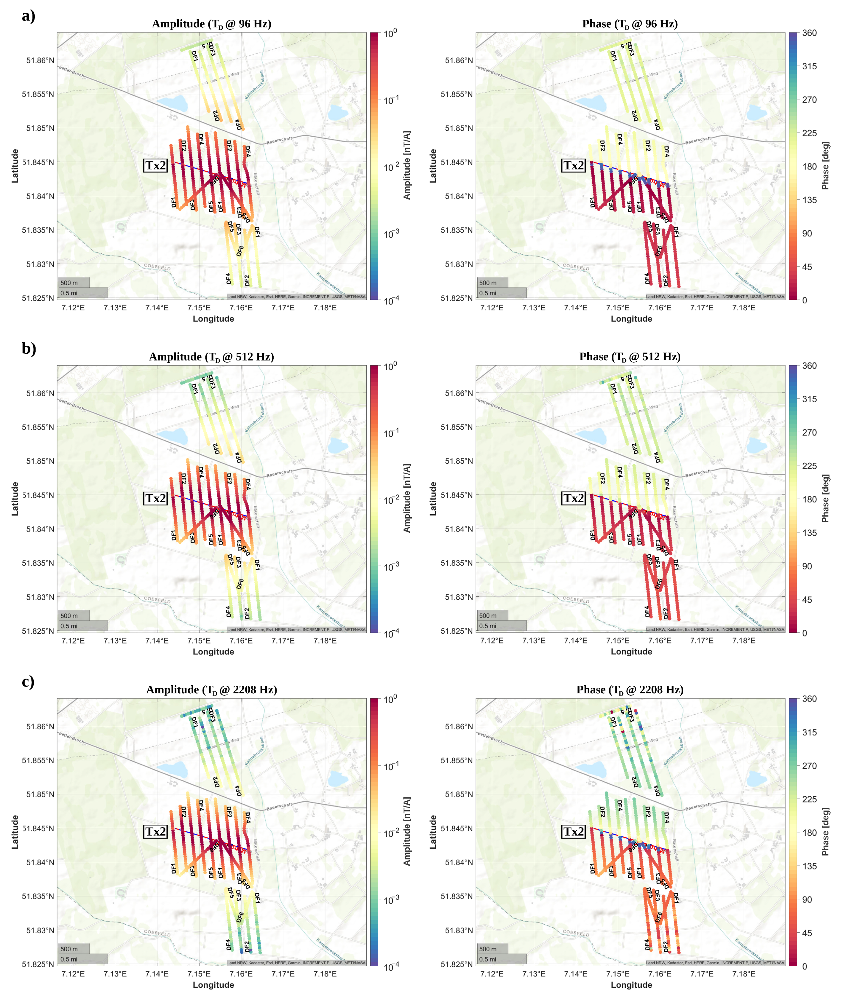
Figure A3.
Spatial distribution of magnetic transfer function estimates at 96 Hz (a), at 512 Hz (b) and at 2208 Hz (c) for active transmitter Tx2. Displayed is the north component. The complex-valued estimates are illustrated in terms of an amplitude (left) and phase (right).
Figure A3.
Spatial distribution of magnetic transfer function estimates at 96 Hz (a), at 512 Hz (b) and at 2208 Hz (c) for active transmitter Tx2. Displayed is the north component. The complex-valued estimates are illustrated in terms of an amplitude (left) and phase (right).
Figure A4.
Spatial distribution of magnetic transfer function estimates at 96 Hz (a), at 512 Hz (b) and at 2208 Hz (c) for active transmitter Tx2. Displayed is the downward component. The complex-valued estimates are illustrated in terms of an amplitude (left) and phase (right).
Figure A4.
Spatial distribution of magnetic transfer function estimates at 96 Hz (a), at 512 Hz (b) and at 2208 Hz (c) for active transmitter Tx2. Displayed is the downward component. The complex-valued estimates are illustrated in terms of an amplitude (left) and phase (right).
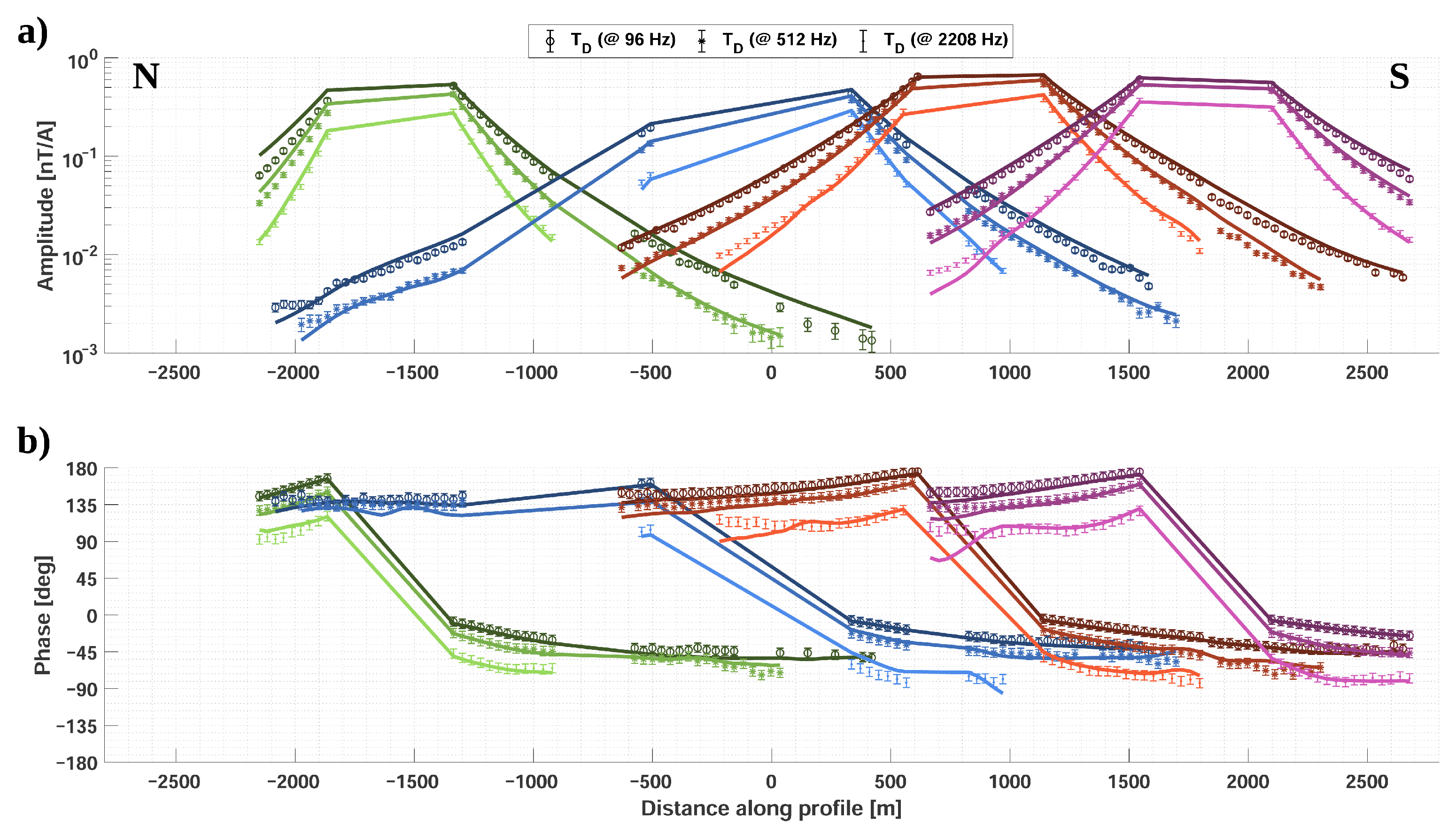
Figure A5.
Transfer function estimates (dots) and final inversion model responses (solid lines) along a profile line (cf.
Figure 6a) at three different binned frequencies (96 Hz, 512 Hz, 2208 Hz) in dependency on running transmitter (Tx1: green, Tx2: blue, Tx3: red, Tx4: purple). Depicted is the horizontal component of the transfer functions
parallel to the profile line in terms of an amplitude (
a) and phase (
b).
Figure A6.
Transfer function estimates (dots) and final inversion model responses (solid lines) along a profile line (cf.
Figure 6a) at three different binned frequencies (96 Hz, 512 Hz, 2208 Hz) in dependency on running transmitter (Tx1: green, Tx2: blue, Tx3: red, Tx4: purple). Depicted is the downward component of the transfer functions
in terms of an amplitude (
a) and phase (
b).
References
- Guéguen, Y.; Palciauskas, V. Introduction to the Physics of Rocks; Princeton University Press: Princeton, NJ, USA, 1994. [Google Scholar]
- Siemon, B.; Christiansen, A.V.; Auken, E. A review of helicopter-borne electromagnetic methods for groundwater exploration. Near Surf. Geophys. 2009, 7, 629–646. [Google Scholar] [CrossRef] [Green Version]
- Smith, R. Electromagnetic induction methods in mining geophysics from 2008 to 2012. Surv. Geophys. 2014, 35, 123–156. [Google Scholar] [CrossRef]
- Bosschart, R.; Seigel, H. Advances in deep penetration airborne electromagnetic methods: Conf. In Proceedings of the 24 International Geological Congress, Montréal, QC, Canada, 21 August 1972; Volume 9, pp. 37–48. [Google Scholar]
- Becker, A.; Hood, P. Airborne electromagnetic methods. Geophys. Geochem. Search Metallic Ores Geol. Surv. Can. Econ. Geol. Rep. 1979, 31, 33–43. [Google Scholar]
- Fountain, D. Airborne electromagnetic systems-50 years of development. Explor. Geophys. 1998, 29, 1–11. [Google Scholar] [CrossRef]
- Elliott, P. The principles and practice of FLAIRTEM. Explor. Geophys. 1998, 29, 58–59. [Google Scholar] [CrossRef]
- Steuer, A.; Smirnova, M.; Becken, M.; Schiffler, M.; Günther, T.; Rochlitz, R.; Yogeshwar, P.; Moerbe, W.; Siemon, B.; Costabel, S.; et al. Comparison of novel semi-airborne electromagnetic data with multi-scale geophysical, petrophysical and geological data from Schleiz, Germany. J. Appl. Geophys. 2020, 182, 104172. [Google Scholar] [CrossRef]
- Mogi, T.; Tanaka, Y.; Kusunoki, K.; Morikawa, T.; Jomori, N. Development of grounded electrical source airborne transient EM (GREATEM). Explor. Geophys. 1998, 29, 61–64. [Google Scholar] [CrossRef]
- Smirnova, M.V.; Becken, M.; Nittinger, C.; Yogeshwar, P.; Mörbe, W.; Rochlitz, R.; Steuer, A.; Costabel, S.; Smirnov, M.Y.; DESMEX Working Group. A novel semiairborne frequency-domain controlled-source electromagnetic system: Three-dimensional inversion of semiairborne data from the flight experiment over an ancient mining area near Schleiz, Germany. Geophysics 2019, 84, E281–E292. [Google Scholar] [CrossRef]
- Nonami, K.; Kendoul, F.; Suzuki, S.; Wang, W.; Nakazawa, D. Autonomous Flying Robots: Unmanned Aerial Vehicles and Micro Aerial Vehicles; Springer Science & Business Media: Tokyo, Japan, 2010. [Google Scholar]
- Garcia-Fernandez, M.; Alvarez-Lopez, Y.; Las Heras, F. Autonomous airborne 3D SAR imaging system for subsurface sensing: UWB-GPR on board a UAV for landmine and IED detection. Remote Sens. 2019, 11, 2357. [Google Scholar] [CrossRef] [Green Version]
- Walter, C.; Braun, A.; Fotopoulos, G. High-resolution unmanned aerial vehicle aeromagnetic surveys for mineral exploration targets. Geophys. Prospect. 2020, 68, 334–349. [Google Scholar] [CrossRef]
- Parshin, A.; Bashkeev, A.; Davidenko, Y.; Persova, M.; Iakovlev, S.; Bukhalov, S.; Grebenkin, N.; Tokareva, M. Lightweight unmanned aerial system for time-domain electromagnetic prospecting—The next stage in applied UAV-Geophysics. Appl. Sci. 2021, 11, 2060. [Google Scholar] [CrossRef]
- Stoll, J.; Noellenburg, R.; Kordes, T.; Becken, M.; Tezkan, B.; Yogeshwar, P.; Bergers, R.; Matzander, U. Semi-Airborne electromagnetics using a multicopter. In Proceedings of the International Workshop on Gravity, Electrical & Magnetic Methods and Their Applications, Xi’an, China, 19–22 May 2019; Society of Exploration Geophysicists and Chinese Geophysical Society: Beijing, China, 2019; pp. 363–366. [Google Scholar]
- Becken, M.; Nittinger, C.G.; Smirnova, M.; Steuer, A.; Martin, T.; Petersen, H.; Meyer, U.; Mörbe, W.; Yogeshwar, P.; Tezkan, B.; et al. DESMEX: A novel system development for semi-airborne electromagnetic exploration. Geophysics 2020, 85, E253–E267. [Google Scholar] [CrossRef]
- Grabert, H. Abrißder Geologie von Nordrhein-Westfalen; Schweizerbart Science Publishers: Stuttgart, Germany, 1998. [Google Scholar]
- Walter, C.; Braun, A.; Fotopoulos, G. Characterizing electromagnetic interference signals for unmanned aerial vehicle geophysical surveys. Geophysics 2021, 86, J21–J32. [Google Scholar] [CrossRef]
- Rousseeuw, P.J. Least median of squares regression. J. Am. Stat. Assoc. 1984, 79, 871–880. [Google Scholar] [CrossRef]
- Key, K. MARE2DEM: A 2-D inversion code for controlled-source electromagnetic and magnetotelluric data. Geophys. J. Int. 2016, 207, 571–588. [Google Scholar] [CrossRef]
- Cai, J.; Yogshwar, P.; Mörbe, W.; Smirnova, M.; Haroon, A.; Becken, M.; Tezkan, B. 2D Joint Inversion Algorithms for Semi-Airborne and LOTEM Data: A Data Application from Eastern Thuringia, Germany. In Proceedings of the 81. Jahrestagung der Deutschen Geophysikalischen Gesellschaft (DGG), Kiel, Germany, 1–5 March 2021. [Google Scholar]
- Constable, S.C.; Parker, R.L.; Constable, C.G. Occam’s inversion: A practical algorithm for generating smooth models from electromagnetic sounding data. Geophysics 1987, 52, 289–300. [Google Scholar] [CrossRef]
- deGroot Hendlin, C.; Constable, S. Occam’s inversion in two dimensions. In SEG Technical Program Expanded Abstracts 1990; Society of Exploration Geophysicists: Tulsa, OK, USA, 1990; pp. 498–500. [Google Scholar]
- Huber, P.J. Robust estimation of a location parameter. In Breakthroughs in Statistics; Springer: New York, NY, USA, 1992; pp. 492–518. [Google Scholar]
- Interpex. IX1D v3 Instruction Manual; Interpex Ltd.: Golden, CO, USA, 2008; pp. 1–133. Available online: http://www.interpex.com/ix1dv3/ix1dv3_version.htm (accessed on 15 October 2021).
Figure 1.
Illustration of the utilized UAS. (a): The Mobile Geophysical Technologies UAS (during operation) composed of a X825 octocopter from Aerialis (1), a compactified Metronix ADU-08e logging device (2), a rigid rod made of carbon fiber (3), a Xsens MTi-G-710 IMU (4), a Bartington Mag-13MSL70 3-axis fluxgate sensor (5) and a Metronix SHFT-02e induction coil triple (6). (b): The UAS with mounted instruments ready for takeoff. Highlighted are the preferential directions of the UAV.
Figure 2.
Map of the semi-airborne EM survey area near Münster (Germany). Displayed is the layout of four HED transmitters (Tx1: green, Tx2: blue, Tx3: red, Tx4: purple) with associated flight areas and flight lines (black).
Figure 2.
Map of the semi-airborne EM survey area near Münster (Germany). Displayed is the layout of four HED transmitters (Tx1: green, Tx2: blue, Tx3: red, Tx4: purple) with associated flight areas and flight lines (black).
Figure 3.
Visualization of the recorded injection current. (a): Time series section of the injected current amperage at transmitter Tx2. (b): Stacked amplitude spectrum of the current amperage at transmitter Tx2. Labeled are amplitudes at the fundamental injection frequency (32 Hz) and at two proximate odd harmonics (96 Hz, 160 Hz). The peak at 8 kHz is due to the pulse-width modulation of the employed transmitter source.
Figure 4.
Spectral comparison of the observed magnetic flux density depending on the distance to the transmitter. (a): Map section displaying transmitter Tx2 and two centered observation points (P1, P2) with different perpendicular distances to the transmitter. (b): Amplitude spectra of the downward component from in-flight induction coil recordings at two different locations (P1: bottom, P2: top). Substantial EM noise bands are marked. (c): Section of the amplitude spectra shown in the central panels. Highlighted are signal amplitudes at point P2 at odd injection harmonics above ambient noise level (black) and below ambient noise level (red).
Figure 5.
Comparison of magnetic transfer functions determined on the basis of different magnetometer sets. Displayed are MFS coil results (black) and SHFT coil triple results on the ground (red) as well as airborne results from the SHFT coil triple (blue) and the fluxgate sensor (yellow) in earth-fixed coordinates (north component (a), east component (b), downward component (c)). The complex-valued transfer functions are displayed in terms of an amplitude (left) and a phase (right). Fluxgate data is displayed only up to 512 Hz.
Figure 6.
Illustration of transfer function estimates. (a): Profile line layout (red dotted line) through the survey area across all four transmitters (red solid lines). Shown are also flight lines (black solid lines) along the profile and linearly approximated transmitter bipoles (blue dashed lines). (b,c): Estimated magnetic transfer functions along a profile line at three different binned frequencies (96 Hz, 512 Hz, 2208 Hz) in dependency on running transmitter (Tx1: green, Tx2: blue, Tx3: red, Tx4: purple). Depicted are amplitudes and phases of the north component.
Figure 7.
A 2D inversion model based on UAV-borne data. (a): Initial homogeneous half-space model (50 m) with a 200 × 200 km bounding box selected for MARE2DEM inversion. Displayed are transmitters (white triangles) and centered receiver points (white circles). The section of the inversion model shown below is represented by the white box. (b): Conductivity distribution along the profile line according to the final inversion result (misfit RMS: 1.50). Marked are a magnetotelluric site (MT) and a geoelectric sounding spot (DC).
Figure 8.
Comparison of the inversion result based on the semi-airborne EM method (black solid line) with 1D inversions resulting from a DC resistivity sounding (blue lines) and a magnetotelluric sounding (magenta lines). Depicted are Occam-type inversions (solid lines) and block inversions (dashed lines).
| Publisher’s Note: MDPI stays neutral with regard to jurisdictional claims in published maps and institutional affiliations. |
© 2022 by the authors. Licensee MDPI, Basel, Switzerland. This article is an open access article distributed under the terms and conditions of the Creative Commons Attribution (CC BY) license (https://creativecommons.org/licenses/by/4.0/).

