
Modeling Shallow Landslide Susceptibility and Assessment of the Relative Importance of Predisposing Factors, through a GIS-Based Statistical Analysis


Abstract
1. Introduction
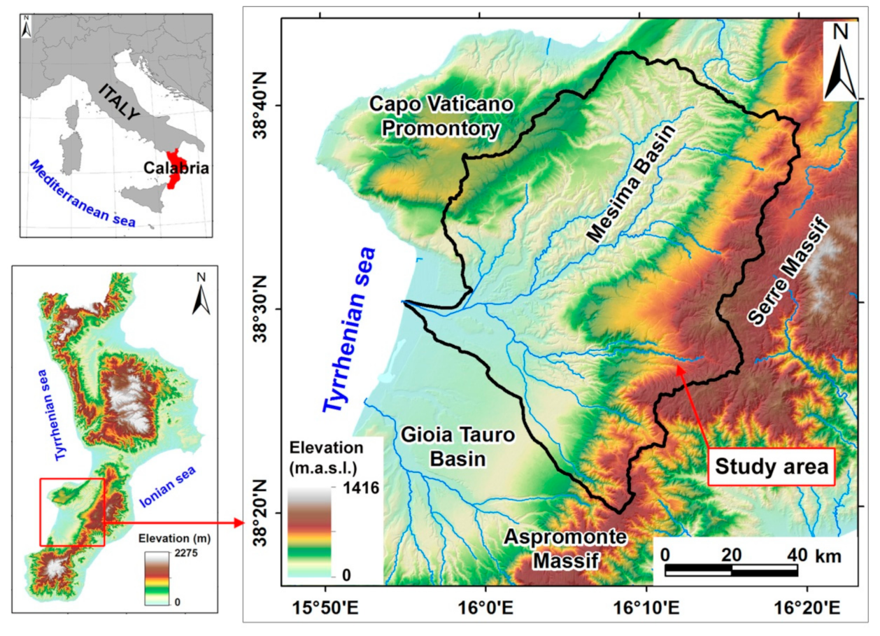
2. Study Area
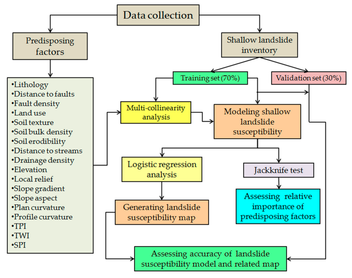
3. Materials and Methods
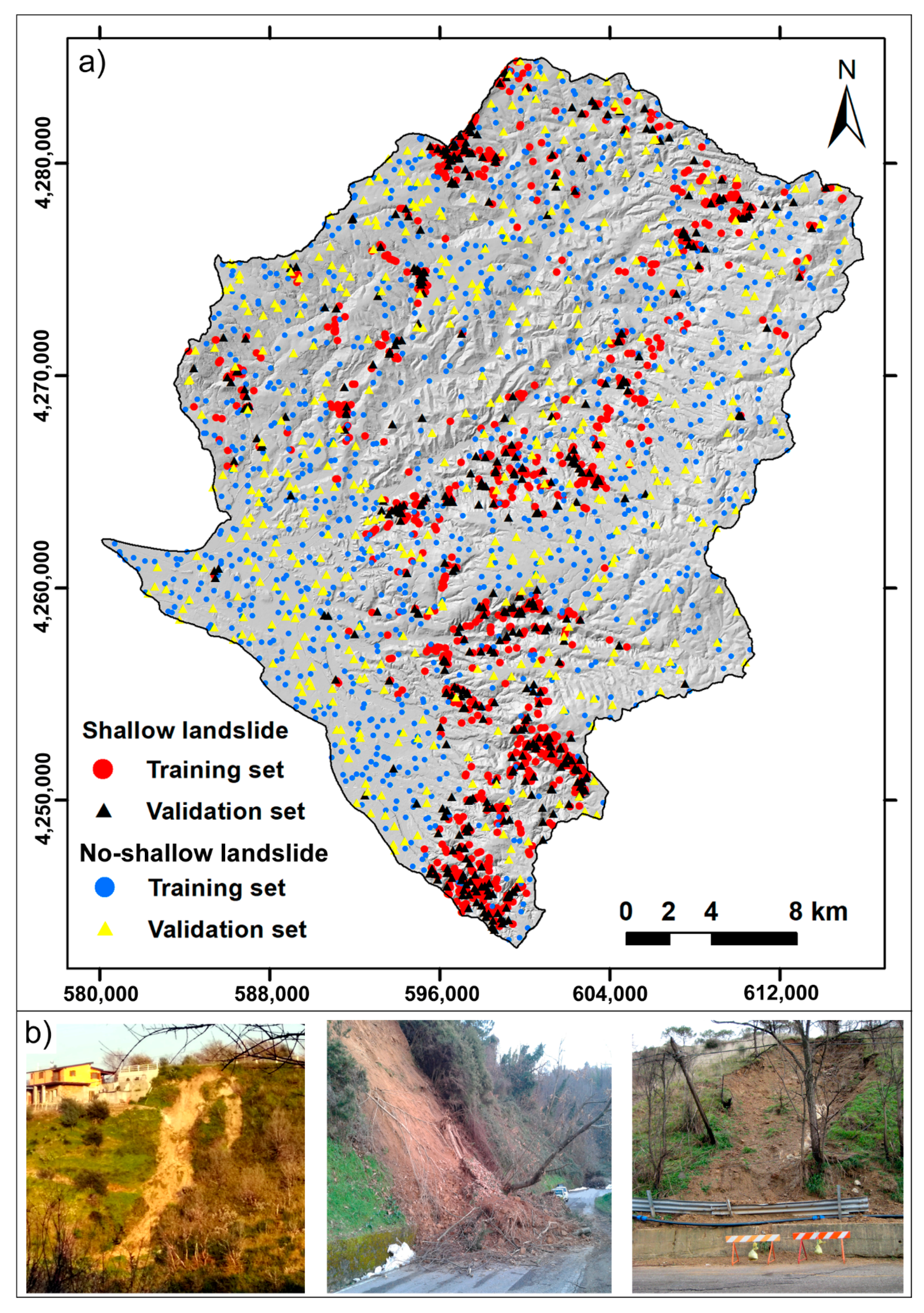
3.1. Shallow Landslide Inventory Map
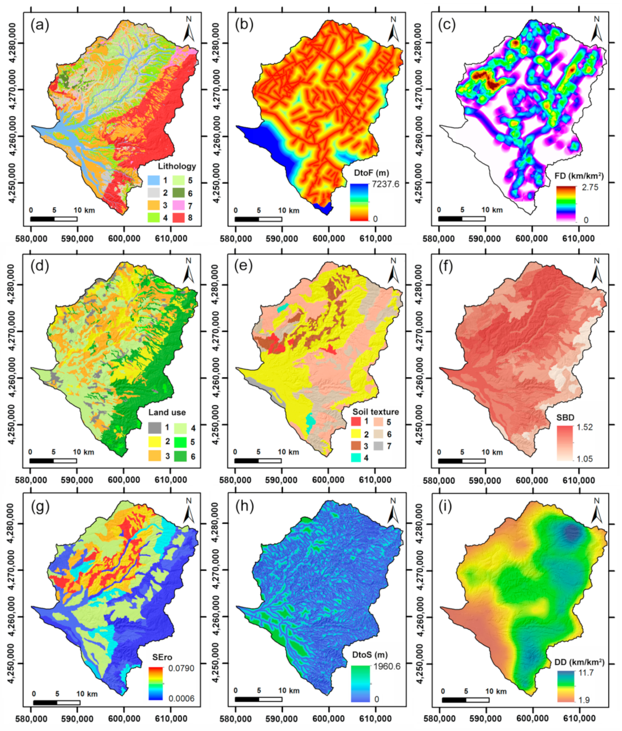
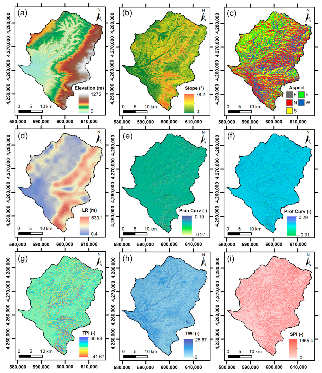
3.2. Shallow Landslide Predisposing Factors
3.3. Shallow Landslide Susceptibility Modeling
3.3.1. Multi-Collinearity Analysis
3.3.2. Logistic Regression Analysis
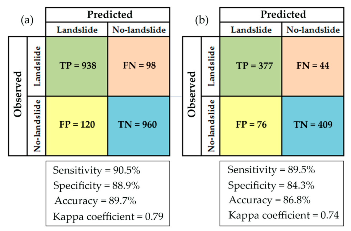
3.3.3. Validation of Susceptibility Model
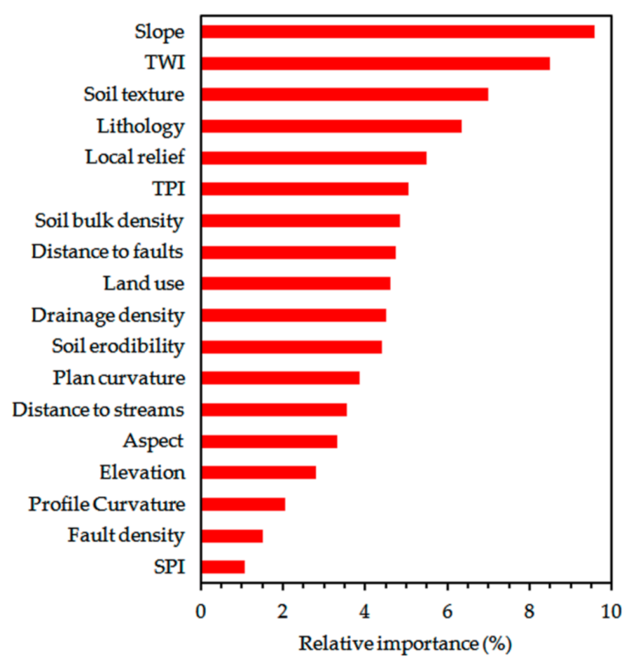
3.3.4. Relative Importance of Predisposing Factors
4. Results
4.1. Detection of Multi-Collinearity between Predisposing Factors
4.2. Assessment of Shallow Landslide Susceptibility
4.3. Performance of the Model and Accuracy of the Susceptibility Map
4.4. Analysis of the Relative Importance of Predisposing Factors
5. Discussion
6. Conclusions
Author Contributions
Funding
Institutional Review Board Statement
Informed Consent Statement
Data Availability Statement
Acknowledgments
Conflicts of Interest
References
- Caine, N. The rainfall intensity: Duration control of shallowlandslides and debris flows. Geogr. Ann. A 1980, 62, 23–27. [Google Scholar]
- Guzzetti, F.; Peruccacci, S.; Rossi, M.; Stark, C.P. The rainfall intensity–duration control of shallow landslides and debris flows: An up-date. Landslides 2008, 5, 3–17. [Google Scholar] [CrossRef]
- Giannecchini, R.; Galanti, Y.; D’Amato Avanzi, G. Critical rainfall thresholds for triggering shallow landslides in the Serchio River Valley (Tuscany, Italy). Nat. Hazards Earth Syst. Sci. 2012, 12, 829–842. [Google Scholar] [CrossRef]
- Hungr, O.; Evans, S.G.; Bovis, M.J.; Hutchinson, J.N. A review of the classification of landslides of the flow type. Environ. Eng. Geosci. 2001, 7, 221–238. [Google Scholar] [CrossRef]
- Zêzere, J.L.; Garcia, R.A.C.; Oliveira, S.C.; Reis, E. Probabilistic landslide risk analysis considering direct costs in the area north of Lisbon (Portugal). Geomorphology 2008, 94, 467–495. [Google Scholar] [CrossRef]
- Salvati, P.; Petrucci, O.; Rossi, M.; Bianchi, C.; Pasqua, A.A.; Guzzetti, F. Gender, age and circumstances analysis of flood and landslide fatalities in Italy. Sci. Total Environ. 2018, 610–611, 867–879. [Google Scholar] [CrossRef]
- Conforti, M.; Ietto, F. An Integrated Approach to Investigate Slope Instability Affecting Infrastructures. Bull. Eng. Geol. Environ. 2019, 78, 2355–2375. [Google Scholar] [CrossRef]
- Van Asch, T.W.J.; Buma, J.; Van Beek, L.P.H. A view on some hydrological triggering systems in landslides. Geomorphology 1999, 30, 25–32. [Google Scholar] [CrossRef]
- Calcaterra, D.; Parise, M. Weathering in the crystalline rocks of Calabria, Italy, and relationships to landslides. Geol. Soc. Lond. Spec. Publ. 2010, 23, 105–130. [Google Scholar] [CrossRef]
- Ietto, F.; Perri, F.; Cella, F. Weathering characterization for landslides modeling in granitoid rock masses of the capo Vaticano promontory (Calabria, Italy). Landslides 2018, 15, 43–62. [Google Scholar] [CrossRef]
- Huggel, C.; Clague, J.J.; Korup, O. Is climate change responsible for changing landslide activity in high mountains? Earth Surf. Process. Land. 2012, 37, 77–91. [Google Scholar] [CrossRef]
- Gariano, S.L.; Guzzetti, F. Landslides in a changing climate. Earth Sci. Rev. 2016, 162, 227–252. [Google Scholar] [CrossRef]
- Guzzetti, F. Landslide fatalities and the evaluation of landslide risk in Italy. Eng. Geol. 2000, 58, 89–107. [Google Scholar] [CrossRef]
- Guzzetti, F.; Cardinali, M.; Reichembach, P. The AVI project: A bibliographical and archive inventory of landslides and floods in Italy. Environ. Manag. 1994, 4, 623–633. [Google Scholar] [CrossRef]
- Salvati, P.; Rossi, M.; Bianchi, C.; Guzzetti, F. Landslide risk to the population of Italy and its geographical and temporal variations. In Extreme Events: Observations, Modeling, and Economics; Chavez, M., Ghil, M., Urrutia-Fucugauchi, J., Eds.; Geophysical Monograph Series; John Wiley & Sons Inc.: Hoboken, NJ, USA, 2016; pp. 177–194. [Google Scholar] [CrossRef]
- Gullà, G.; Antronico, L.; Iaquinta, P.; Terranova, O. Susceptibility and triggering scenarios at a regional scale for shallow landslides. Geomorphology 2008, 99, 39–58. [Google Scholar] [CrossRef]
- Lucà, F.; Robustelli, G.; Conforti, M.; Fabbricatore, D. Geomorphological Map of the Crotone Province (Calabria, South Italy). J. Maps 2011, 7, 375–390. [Google Scholar] [CrossRef][Green Version]
- Iovine, G.; Greco, R.; Gariano, S.L.; Pellegrino, A.D.; Terranova, O.G. Shallow-landslide susceptibility in the Costa Viola mountain ridge (southern Calabria, Italy) with considerations on the role of causal factors. Nat. Hazards 2014, 73, 111–136. [Google Scholar] [CrossRef]
- Borrelli, L.; Cofone, G.; Coscarelli, R.; Gullà, G. Shallow landslides triggered by consecutive rainfall events at Catanzaro strait (Calabria-Southern Italy). J. Maps 2015, 11, 730–744. [Google Scholar] [CrossRef]
- Gariano, S.L.; Petrucci, O.; Guzzetti, F. Changes in the occurrence of rainfall-induced landslides in Calabria, southern Italy, in the 20th century. Nat. Hazards Earth Sys. 2015, 15, 2313–2330. [Google Scholar] [CrossRef]
- Ietto, F.; Perri, F.; Fortunato, G. Lateral spreading phenomena and weathering processes from the Tropea area (Calabria, Southern Italy). Environ. Earth Sci. 2015, 73, 4595–4608. [Google Scholar] [CrossRef]
- Conforti, M.; Rago, V.; Muto, F.; Versace, P. GIS-based statistical analysis for assessing shallow-landslide susceptibility along the highway in Calabria (Southern Italy). Rend. Online Soc. Geol. Ital. 2016, 39, 155–158. [Google Scholar] [CrossRef]
- Conforti, M.; Buttafuoco, G. Assessing space-time variations of denudation processes and related soil loss from 1955 to 2016 in southern Italy (Calabria region). Environ. Earth Sci. 2017, 76, 457. [Google Scholar] [CrossRef]
- Fell, R.; Corominas, J.; Bonnard, C.; Cascini, L.; Leroi, E.; Savage, W.Z. Guidelines for landslide susceptibility, hazard and risk zoning for land-use planning. Eng. Geol. 2008, 102, 99–111. [Google Scholar]
- Pourghasemi, H.R.; Pradhan, B.; Gokceoglu, C. Application of fuzzy logic and analytical hierarchy process (AHP) to landslide susceptibility mapping at Haraz watershed. Nat. Hazards 2012, 63, 965–996. [Google Scholar] [CrossRef]
- Baeza, C.; Corominas, J. Assessment of shallow landslide susceptibility by means of multivariate statistical techniques. Earth Surf. Process. Landf. 2001, 26, 1251–1263. [Google Scholar] [CrossRef]
- Schlögel, R.; Marchesini, I.; Alvioli, M.; Reichenbach, P.; Rossi, M.; Malet, J.P. Optimizing landslide susceptibility zonation: Effects of DEM spatial resolution and slope unit delineation on logistic regression models. Geomorphology 2018, 301, 10–20. [Google Scholar] [CrossRef]
- Montgomery, D.R.; Dietrich, W.E. A physically based model for the topographic control on shallow landsliding. Water Resour. Res. 1994, 30, 1153–1171. [Google Scholar] [CrossRef]
- Park, S.; Choi, C.; Kim, B.; Kim, J. Landslide susceptibility mapping using frequency ratio, analytic hierarchy process, logistic regression, and artificial neural network methods at the Inje Area, Korea. Environ. Earth Sci. 2013, 68, 1443–1464. [Google Scholar] [CrossRef]
- Yalcin, A. GIS-based landslide susceptibility mapping using analytical hierarchy process and bivariate statistics in Ardesen (Turkey): Comparisons of results and confirmations. Catena 2008, 72, 1–12. [Google Scholar] [CrossRef]
- Corominas, J.; Van Westen, C.; Frattini, P.; Cascini, L.; Malet, J.P.; Fotopoulou, S.; Catani, F.; Eeckhaut, V.D.; Mavrouli, O.; Agliardi, F.; et al. Recommendations for the quantitative analysis of landslide risk. Eng. Geol. Environ. 2014, 73, 209–263. [Google Scholar] [CrossRef]
- Zhou, C.; Yin, K.; Cao, Y.; Ahmed, B.; Li, Y.; Catani, F.; Pourghasemi, H.R. Landslide susceptibility modeling applying machine learning methods: A case study from Longju in the Three Gorges Reservoir area, China. Comput. Geosci. 2018, 112, 23–37. [Google Scholar] [CrossRef]
- Akgun, A.; Dag, S.; Bulut, F. Landslide susceptibility mapping for a landslide-prone area Findikli, NE of Turkey by likelihood-frequency ratio and weighted linear combination models. Environ. Geol. 2008, 546, 1127–1143. [Google Scholar] [CrossRef]
- Kayastha, P.; Dhital, M.R.; De Smedt, F. Application of the analytical hierarchy process (AHP) for landslide susceptibility mapping: A case study from the Tinau watershed, west Nepal. Comput. Geosci. 2013, 52, 398–408. [Google Scholar] [CrossRef]
- Abedini, M.; Tulabi, S. Assessing LNRF, FR, and AHP models in landslide susceptibility mapping index: A comparative study of Nojian watershed in Lorestan province, Iran. Environ. Earth Sci. 2018, 7711, 405. [Google Scholar] [CrossRef]
- Saaty, T.L. The Analytic Hierarchy Process; McGraw-Hill, Ed.; Scientific Research Publishing: New York, NY, USA, 1980. [Google Scholar]
- Ruff, M.; Czurda, K. Landslide susceptibility analysis with a heuristic approach in the Eastern Alps (Vorarlberg, Austria). Geomorphology 2008, 94, 314–324. [Google Scholar] [CrossRef]
- Ciurleo, M.; Mandaglio, M.C.; Moraci, N. Landslide susceptibility assessment by TRIGRS in a frequently affected shallow instability area. Landslides 2019, 16, 175–188. [Google Scholar] [CrossRef]
- Park, D.W.; Nikhil, N.V.; Lee, S.R. Landslide and debris flow susceptibility zonation using TRIGRS for the 2011 Seoul landslide event. Nat. Hazards Earth Syst. Sci. 2013, 13, 2833–2849. [Google Scholar] [CrossRef]
- Dou, H.; Han, T.; Gong, X.; Zhang, J. Probabilistic slope stability analysis considering the variability of hydraulic conductivity under rainfall infiltration–redistribution conditions. Eng. Geol. 2014, 183, 1–13. [Google Scholar]
- Pham, B.T.; Tien Bui, D.; Pourghasemi, H.R.; Indra, P.; Dholakia, M.B. Landslide susceptibility assessment in the Uttarakhand area (India) using GIS: A comparison study of prediction capability of naıve Bayes, multilayer perceptron neural networks, and functional trees methods. Theor. Appl. Climatol. 2017, 128, 255–273. [Google Scholar] [CrossRef]
- Yilmaz, I. Landslide susceptibility mapping using frequency ratio, logistic regression, artificial neural networks and their comparison: A case study from Kat landslides (Tokat-Turkey). Comput. Geosci. 2009, 35, 1125–1138. [Google Scholar] [CrossRef]
- Regmi, A.D.; Devkota, K.C.; Yoshida, K.; Pradhan, B.; Pourghasemi, H.R.; Kumamoto, T.; Akgun, A. Application of frequency ratio, statistical index, and weights-of-evidence models and their comparison in landslide susceptibility mapping in Central Nepal Himalaya. Arab. J. Geosci. 2014, 7, 725–742. [Google Scholar] [CrossRef]
- Youssef, A.M.; Pourghasemi, H.R.; Pourtaghi, Z.S.; Al-Katheeri, M.M. Landslide susceptibility mapping using random forest, boosted regression tree, classification and regression tree, and general linear models and comparison of their performance at Wadi Tayyah Basin, Asir Region, Saudi Arabia. Landslides 2016, 13, 1–18. [Google Scholar]
- Wang, L.J.; Guo, M.; Sawada, K.; Lin, J.; Zhang, J. A comparative study of landslide susceptibility maps using logistic regression, frequency ratio, decision tree, weights of evidence and artificial neural network. Geosci. J. 2016, 20, 117–136. [Google Scholar] [CrossRef]
- Pourghasemi, H.R.; Pradhan, B.; Gokceoglu, C.; Mohammadi, M.; Moradi, H.R. Application of weights-of-evidence and certainty factor models and their comparison in landslide susceptibility mapping at Haraz watershed, Iran. Arab. J. Geosci. 2013, 6, 2351–2365. [Google Scholar] [CrossRef]
- Devkota, K.C.; Regmi, A.D.; Pourghasemi, H.R.; Yoshida, K.; Pradhan, B.; Ryu, I.C.; Dhital, M.R.; Althuwaynee, O.F. Landslide susceptibility mapping using certainty factor, index of entropy and logistic regression models in GIS and their comparison at Mugling-Narayanghat road section in Nepal Himalaya. Nat. Hazards 2013, 65, 135–165. [Google Scholar] [CrossRef]
- Althuwaynee, O.F.; Pradhan, B.; Lee, S. Application of an evidential belief function model in landslide susceptibility mapping. Comput. Geosci. 2012, 44, 120–135. [Google Scholar] [CrossRef]
- Pourghasemi, H.R.; Kerle, N. Random forests and evidential belief function-based landslide susceptibility assessment in Western Mazandaran Province, Iran. Environ. Earth Sci. 2016, 75, 1–17. [Google Scholar] [CrossRef]
- Conforti, M.; Robustelli, G.; Muto, F.; Critelli, S. Application and Validation of Bivariate GIS-Based Landslide Susceptibility Assessment for the Vitravo River Catchment (Calabria, South Italy). Nat. Hazards 2012, 61, 127–141. [Google Scholar] [CrossRef]
- Chen, T.; Niu, R.; Jia, X. A comparison of information value and logistic regression models in landslide susceptibility mapping by using GIS. Environ. Earth Sci. 2016, 75, 867. [Google Scholar] [CrossRef]
- Youssef, A.M.; Al-Kathery, M.; Pradhan, B. Landslide susceptibility mapping at al-hasher area, Jizan (Saudi Arabia) using gis-based frequency ratio and index of entropy models. Geosci. J. 2015, 19, 113–134. [Google Scholar] [CrossRef]
- Hong, H.; Chen, W.; Xu, C.; Youssef, A.M.; Pradhan, B.T.; Bui, D. Rainfall-induced landslide susceptibility assessment at the Chongren area (China) using frequency ratio, certainty factor, and index of entropy. Geocarto Int. 2017, 32, 139–154. [Google Scholar] [CrossRef]
- Felicísimo, Á.M.; Cuartero, A.; Remondo, J.; Quirós, E. Mapping landslide susceptibility with logistic regression, multiple adaptive regression splines, classification and regression trees, and maximum entropy methods: A comparative study. Landslides 2013, 10, 175–189. [Google Scholar] [CrossRef]
- Pourghasemi, H.R.; Rossi, M. Landslide susceptibility modeling in a landslide prone area in Mazandarn Province, north of Iran: A comparison between GLM, GAM, MARS, and M-AHP methods. Theor. Appl. Climatol. 2016, 130, 609–633. [Google Scholar] [CrossRef]
- Conforti, M.; Pascale, S.; Robustelli, G.; Sdao, F. Evaluation of prediction capability of the artificial neural networks for mapping landslide susceptibility in the Turbolo River catchment (northern Calabria, Italy). Catena 2014, 113, 236–250. [Google Scholar] [CrossRef]
- Tien Bui, D.; Tuan, T.A.; Klempe, H.; Pradhan, B.; Revhaug, I. Spatial prediction models for shallow landslide hazards: A comparative assessment of the efficacy of support vector machines, artificial neural networks, kernel logistic regression, and logistic model tree. Landslides 2016, 13, 361–378. [Google Scholar] [CrossRef]
- Park, N.-W. Using maximum entropy modeling for landslide susceptibility mapping with multiple geoenvironmental data sets. Environ. Earth Sci. 2015, 73, 937–949. [Google Scholar] [CrossRef]
- Chen, W.; Pourghasemi, H.R.; Naghibi, S.A. A comparative study of landslide susceptibility maps produced using support vector machine with different kernel functions and entropy data mining models in China. Bull. Eng. Geol. Environ. 2018, 77, 647–664. [Google Scholar] [CrossRef]
- Catani, F.; Lagomarsino, D.; Segoni, S.; Tofani, V. Landslide susceptibility estimation by random forests technique: Sensitivity and scaling issues. Nat. Hazards Earth Syst. Sci. 2013, 13, 2815–2831. [Google Scholar] [CrossRef]
- Chen, W.; Xie, X.; Wang, J.; Pradhan, B.; Hong, H.; Bui, D.T.; Duan, Z.; Ma, J. A comparative study of logistic model tree, random forest, and classification and regression tree models for spatial prediction of landslide susceptibility. Catena 2017, 151, 147–160. [Google Scholar] [CrossRef]
- Tien Bui, D.; Pradhan, B.; Lofman, O.; Revhaug, I.; Dick, O.B. Landslide susceptibility mapping at Hoa Binh province (Vietnam) using an adaptive neuro-fuzzy inference system and GIS. Comput. Geosci. 2012, 45, 199–211. [Google Scholar] [CrossRef]
- Pradhan, B. A comparative study on the predictive ability of the decision tree, support vector machine and neuro-fuzzy models in landslide susceptibility mapping using GIS. Comput. Geosci. 2013, 51, 350–365. [Google Scholar] [CrossRef]
- Peng, L.; Niu, R.; Huang, B.; Wu, X.; Zhao, Y.; Ye, R. Landslide susceptibility mapping based on rough set theory and support vector machines: A case of the Three Gorges area, China. Geomorphology 2014, 204, 287–301. [Google Scholar] [CrossRef]
- Pourghasemi, H.; Gayen, A.; Park, S.; Lee, C.-W.; Lee, S. Assessment of Landslide-Prone Areas and Their Zonation Using Logistic Regression, LogitBoost, and NaïveBayes Machine-Learning Algorithms. Sustainability 2018, 10, 3697. [Google Scholar] [CrossRef]
- Oh, H.-J.; Pradhan, B. Application of a neuro-fuzzy model to landslide-susceptibility mapping for shallow landslides in a tropical hilly area. Comput. Geosci. 2011, 37, 1264–1276. [Google Scholar] [CrossRef]
- Lombardo, L.; Cama, M.; Conoscenti, C.; Märker, M.; Rotigliano, E. Binary logistic regression versus stochastic gradient boosted decision trees in assessing landslide susceptibility for multiple-occurring landslide events: Application to the 2009 storm event in Messina (Sicily, Southern Italy). Nat. Hazards 2015, 79, 1621–1648. [Google Scholar] [CrossRef]
- Hong, H.; Pradhan, B.; Xu, C.; Tien Bui, D. Spatial prediction of landslide hazard at the Yihuang area (China) using two-class kernel logistic regression, alternating decision tree and support vector machines. Catena 2015, 133, 266–281. [Google Scholar] [CrossRef]
- Van Westen, C.J.; Castellanos Abella, E.A.; Sekhar, L.K. Spatial data for landslide susceptibility, hazards and vulnerability assessment: An overview. Eng. Geol. 2008, 102, 112–131. [Google Scholar] [CrossRef]
- Huang, F.; Yao, C.; Liu, W.; Li, Y.; Liu, X. Landslide susceptibility assessment in the Nantian area of China: A comparison of frequency ratio model and support vector machine. Geomat. Nat. Hazards Risk 2018, 9, 919–938. [Google Scholar] [CrossRef]
- Arabameri, A.; Pradhan, B.; Lombardo, L. Comparative assessment using boosted regression trees, binary logistic regression, frequency ratio and numerical risk factor for gully erosion susceptibility modelling. Catena 2019, 183, 104223. [Google Scholar] [CrossRef]
- Guo, Z.; Yin, K.; Gui, L.; Liu, Q.; Huang, F.; Wang, T. Regional rainfall warning system for landslides with creep deformation in three gorges using a statistical black box model. Sci. Rep. 2019, 9, 8962. [Google Scholar] [CrossRef]
- Ayalew, L.; Yamagishi, H. The application of GIS-based logistic regression for landslide susceptibility mapping in the Kakuda Yahiko Mountains, Central Japan. Geomorphology 2005, 65, 15–31. [Google Scholar] [CrossRef]
- Kavzoglu, T.; Kutlug Sahin, E.; Colkesen, I. Selecting optimal conditioning factors in shallow translational landslide susceptibility mapping using genetic algorithm. Eng. Geol. 2015, 192, 101–112. [Google Scholar] [CrossRef]
- Wang, Q.; Wang, D.; Yong, H.; Wang, Z.; Zhang, L.; Guo, Q.; Wei, C.; Sang, M. Landslide Susceptibility Mapping Based on Selected Optimal Combination of Landslide Predisposing Factors in a Large Catchment. Sustainability 2015, 7, 16653–16669. [Google Scholar] [CrossRef]
- Costanzo, D.; Rotigliano, E.; Irigaray, C.; Jiménez-Perálvarez, J.D.; Chacón, J. Factors selection in landslide susceptibility modelling on large scale following the GIS matrix method: Application to the river Beiro basin (Spain). Nat. Hazards Earth Syst. Sci. 2012, 12, 327–340. [Google Scholar] [CrossRef]
- Wu, X.; Niu, R.; Ren, F.; Peng, L. Landslide susceptibility mapping using rough sets and back-propagation neural networks in the three gorges, china. Environ. Earth Sci. 2013, 70, 1307–1318. [Google Scholar] [CrossRef]
- Conforti, M.; Ietto, F. Influence of tectonics and morphometric features on the landslide distribution: A case study from the Mesima basin (Calabria, south Italy). J. Earth Sci. 2020, 31, 393–409. [Google Scholar] [CrossRef]
- Ietto, F.; Cantasano, N.; Salvo, F. The quality of life conditioning with reference to the local environmental management: A pattern in Bivona country (Calabria, Southern Italy). Ocean. Coast. Manag. 2014, 102, 340–349. [Google Scholar] [CrossRef]
- Amodio Morelli, L.; Bonardi, G.; Colonna, V.; Dietrich, D.; Giunta, G.; Ippolito, F.; Liguori, V.; Lorenzoni, S.; Paglionico, A.; Perrone, V.; et al. L’Arco Calabro-peloritano nell’orogene Appenninico-Maghrebide. Mem. Soc. Geol. Ital. 1976, 17, 1–60. (In Italian) [Google Scholar]
- Brutto, F.; Muto, F.; Loreto, M.F.; De Paola, N.; Tripodi, V.; Critelli, S.; Facchin, L. The Neogene-Quaternary geodynamic evolution of the central Calabrian Arc: A case study from the western Catanzaro Trough basin. J. Geodyn. 2016, 102, 95–114. [Google Scholar] [CrossRef]
- Dewey, J.F.; Helman, M.L.; Knott, S.D.; Turco, E.; Hutton, D.H.W. Kinematics of the Western Mediterranean. Geol. Soc. Lond. Spec. Publ. 1989, 45, 265–284. [Google Scholar] [CrossRef]
- Pezzino, A.; Angì, G.; Fazio, E.; Fiannacca, P.; Lo Giudice, A.; Ortolano, G.; Punturo, R.; Cirrincione, R.; De Vuono, E. Alpine Metamorphism in the Aspromonte Massif: Implications for a New Framework for the Southern Sector of the Calabria-Peloritani Orogen, Italy. Int. Geol. Rev. 2008, 50, 423–441. [Google Scholar] [CrossRef]
- Critelli, S.; Le Pera, E. Tectonic evolution of the Southern Apennines thrust-belt (Italy) as reflected in modal compositions of Cenozoic sandstone. J. Geol. 1995, 103, 95–105. [Google Scholar] [CrossRef]
- Tortorici, L.; Monaco, C.; Tansi, C.; Cocina, O. Recent and Active Tectonics in the Calabrian Arc (Southern Italy). Tectonophysics 1995, 243, 37–55. [Google Scholar] [CrossRef]
- Tansi, C.; Muto, F.; Critelli, S.; Iovine, G. Neogene-Quaternary Strike-Slip Tectonics in the Central Calabrian Arc (Southern Italy). J. Geodyn. 2007, 43, 393–414. [Google Scholar] [CrossRef]
- Monaco, C.; Tortorici, L. Active Faulting in the Calabrian Arc and Eastern Sicily. J. Geodyn. 2000, 29, 407–424. [Google Scholar] [CrossRef]
- Ietto, F.; Bernasconi, M.P. The cliff bordering the northwestern margin of the Mesima basin (Southern Calabria) is of Pleistocene age. Geogr. Fis. Dinam. Quat. 2005, 28, 205–210. [Google Scholar]
- Antonioli, F.; Ferranti, L.; Lambeck, K.; Kershaw, S.; Verrubbi, V.; Dai Pra, G. Late Pleistocene to Holocene record of chaning uplift rates in southern Calabria and northestern Siciliy (southern Italy, central Mediterranean sea). Tectonophysics 2006, 422, 23–40. [Google Scholar] [CrossRef]
- Antonioli, F.; Ferranti, L.; Fontana, A.; Amorosi, A.; Bondesan, A.; Braitenberg, C.; Dutton, C.; Fontolan, G.; Furlani, S.; Lambeck, K.; et al. Holocene relative sea-level changes and vertical movements along the Italian and Istrian coastlines. Quat. Int. 2009, 206, 102–133. [Google Scholar] [CrossRef]
- Ietto, A.; Ietto, F. Age and history of the weathering of granitoids in southern Calabria (Italy). Geogr. Fis. Dinam. Quat. 2004, 27, 37–45. [Google Scholar]
- Perri, F.; Ietto, F.; Le Pera, E.; Apollaro, C. Weathering Processes Affecting Granitoid Profiles of Capo Vaticano (Calabria, Southern Italy) Based on Petrographic, Mineralogic and Reaction Path Modelling Approaches. Geol. J. 2016, 51, 368–386. [Google Scholar] [CrossRef]
- Ietto, F.; Perri, F.; Cella, F. Geotechnical and Landslide Aspects in Weathered Granitoid Rock Masses (Serre Massif, Southern Calabria, Italy). Catena 2016, 145, 301–315. [Google Scholar] [CrossRef]
- Ferranti, L.; Antonioli, F.; Mauz, B.; Amorosi, A.; Dai Pra, G.; Mastronuzzi, G.; Monaco, C.; Orrù, P.; Pappalardo, M.; Radtke, U.; et al. Markers of the Last Interglacial Sea-Level High Stand along the Coast of Italy: Tectonic Implications. Quat. Int. 2006, 145–146, 30–54. [Google Scholar] [CrossRef]
- USDA. Keys to soil taxonomy. In Soil Survey Staff, 12th ed.; USDA, Natural Resources Conservation Service: Washington, DC, USA, 2014; p. 372. [Google Scholar]
- ARSSA. Carta dei suoli della regione Calabria—Scala 1:250000. In Monografia Divulgativa; Servizio Agropedologia; ARSSA—Agenzia Regionale per lo Sviluppo e per i Servizi in Agricoltura, Rubbettino Publisher: Soveria Mannelli, Italy, 2003; 387p. [Google Scholar]
- Conforti, M.; Matteucci, G.; Buttafuoco, G. Organic carbon and total nitrogen topsoil stocks, biogenetic natural reserve ‘Marchesale’ (Calabria region, southern Italy). J. Maps 2017, 13, 91–99. [Google Scholar] [CrossRef]
- Ietto, F.; Bernasconi, M.P. Evidences of Fossil Landslides from the Lower Pleistocene on the Northwestern Margin of the Mesima Basin (Southern Calabria, Italy). Rend. Online Soc. Geol. Ital. 2016, 38, 65–68. [Google Scholar] [CrossRef]
- Cruden, D.M.; Varnes, D.J. Landslides: Investigation and Mitigation. Chapter 3—Landslide Types and Processes. Transp. Res. Board Spec. Rep. 1996, 247, 36–75. [Google Scholar]
- Chung, C.J.F.; Fabbri, A.G. Validation of spatial prediction models for landslide hazard mapping. Nat. Hazards 2003, 30, 451–472. [Google Scholar] [CrossRef]
- Dou, J.; Tien Bui, D.P.; Yunus, A.; Jia, K.; Song, X.; Revhaug, I.; Xia, H.; Zhu, Z. Optimization of Causative Factors for Landslide Susceptibility Evaluation Using Remote Sensing and GIS Data in Parts of Niigata, Japan. PLoS ONE 2015, 10, e0133262. [Google Scholar] [CrossRef]
- Reichenbach, P.; Rossi, M.; Malamud, B.D.; Mihir, M.; Guzzetti, F. A review of statistically-based landslide susceptibility models. Earth Sci. Rev. 2018, 180, 60–91. [Google Scholar] [CrossRef]
- Gholami, M.; Ghachkanlu, E.N.; Khosravi, K.; Pirasteh, S. Landslide prediction capability by comparison of frequency ratio, fuzzy gamma and landslide index method. J. Earth Syst. Sci. 2019, 128, 42. [Google Scholar] [CrossRef]
- ARSSA. Carta del rischio di erosione attuale e potenziale della regione Calabria. Scala 1:250,000. In Servizio Agropedologia; Monografia Divulgativa; ARSSA, Agenzia Regionale per lo Sviluppo e per i Servizi in Agricoltura, Settore Servizi Tecnici di Supporto, Editrice Cerbone: Napoli, Italy, 2005; 107p. [Google Scholar]
- Olaya, V.A. Gentle Introduction to SAGA GIS; The SAGA User Group EV: Göettingen, Germany, 2004. [Google Scholar]
- Molin, P.; Fubelli, G.; Dramis, F. The Tectonic Influence on Drainage Evolution in an Uplifting Area: The Case of the Sila Greca (Calabria, Italy). Geogr. Fis. Dinam. Quat. 2012, 35, 49–60. [Google Scholar]
- Scotti, V.N.; Molin, P.; Faccenna, C.; Soligo, M.; Casas-Sainz, A. The Influence of Surface and Tectonic Processes on Landscape Evolution of the Iberian Chain (Spain): Quantitative Geomorphological Analysis and Geochronology. Geomorphology 2014, 206, 37–57. [Google Scholar] [CrossRef]
- Rahmati, O.; Tahmasebipour, N.; Haghizadeh, A.; Pourghasemi, H.R.; Feizizadeh, B. Evaluating the influence of geo-environmental factors on gully erosion in a semi-arid region of Iran: An integrated framework. Sci. Total Environ. 2017, 579, 913–927. [Google Scholar] [CrossRef] [PubMed]
- Polykretis, C.; Chalkias, C. Comparison and evaluation of landslide susceptibility maps obtained from weight of evidence, logistic regression, and artificial neural network models. Nat. Hazards 2018, 93, 249–274. [Google Scholar] [CrossRef]
- Bai, S.B.; Wang, J.; Lü, G.N.; Zhou, P.G.; Hou, S.S.; Xu, S.N. GIS-based logistic regression for landslide susceptibility mapping of the Zhongxian segment in the Three Gorges area, China. Geomorphology 2010, 115, 23–31. [Google Scholar] [CrossRef]
- Menard, S. Applied Logistic Regression Analysis (Quantitative Applications in the Social Sciences); Sage Publications: New York, NY, USA, 1995; 111p. [Google Scholar]
- Hosmer, D.W.; Lemeshow, S. Applied Logistic Regression; Wiley: Hoboken, NJ, USA, 2000; 528p. [Google Scholar]
- Carrara, A. Uncertainty in evaluating landslide hazard and risk. In Prediction and Perception of Natural Hazards; Nemec, J., Nigs, J.M., Siccardi, F., Eds.; Kluwer: Dordrecht, The Netherlands, 1983; pp. 101–111. [Google Scholar]
- Beguería, S. Validation and evaluation of predictive models in hazard assessment and risk management. Nat. Hazards 2006, 37, 315–329. [Google Scholar] [CrossRef]
- Fawcett, T. An introduction to ROC analysis. Pattern Recognit. Lett. 2006, 27, 861–874. [Google Scholar] [CrossRef]
- Williams, G. Data Mining with Rattle and R: The Art of Excavating Data for Knowledge Discovery; Springer: Dordrecht, The Netherlands, 2011. [Google Scholar]
- Allouche, O.; Tsoar, A.; Kadmon, R. Assessing the accuracy of species distribution models: Prevalence, kappa and the true skill statistic (TSS). J. Appl. Ecol. 2006, 43, 1223–1232. [Google Scholar] [CrossRef]
- Saito, H.; Nakayama, D.; Matsuyama, H. Comparison of landslide susceptibility based on a decision-tree model and actual landslide occurrence: The Akaishi Mountains, Japan. Geomorphology 2009, 109, 108–121. [Google Scholar] [CrossRef]
- Landis, J.R.; Koch, G.G. The measurement of observer agreement for categorical data. Biometrics 1977, 33, 159–174. [Google Scholar] [CrossRef]
- Convertino, M.; Troccoli, A.; Catani, F. Detecting fingerprints of landslide drivers: A Max Ent model. J. Geophys. Res. Earth Surf. 2013, 118, 1367–1386. [Google Scholar] [CrossRef]
- Kornejady, A.; Ownegh, M.; Bahremand, A. Landslide susceptibility assessment using maximum entropy model with two different data sampling methods. Catena 2017, 152, 144–162. [Google Scholar] [CrossRef]
- Du, G.L.; Zhang, Y.S.; Iqbal, J.; Yang, Z.H.; Yao, X. Landslide susceptibility mapping using an integrated model of information value method and logistic regression in the Bailongjiang watershed, Gansu Province, China. J. Mt. Sci. 2017, 14, 249–268. [Google Scholar] [CrossRef]
- Tsangaratos, P.; Ilia, I. Comparison of a logistic regression and Naïve Bayes classifier in landslide susceptibility assessments: The influence of models complexity and training dataset size. Catena 2016, 145, 164–179. [Google Scholar] [CrossRef]
- Sarkar, S.; Kanungo, D.P.; Patra, A.K.; Pushpendra, K. GIS based spatial data analysis for landslide susceptibility mapping. J. Mt. Sci. 2008, 5, 52–62. [Google Scholar] [CrossRef]
- Pham, B.T.; Tien Bui, D.; Prakash, I.; Dholakia, M.B. Rotation forest fuzzy rule-based classifier ensemble for spatial prediction of landslides using GIS. Nat. Hazards 2016, 83, 97–127. [Google Scholar] [CrossRef]
- Lan, H.X.; Zhou, C.H.; Wang, L.J.; Zhang, H.Y.; Li, R.H. Landslide hazard spatial analysis and prediction using GIS in the Xiaojiang watershed, Yunnan, China. Eng. Geol. 2004, 76, 109–128. [Google Scholar] [CrossRef]
- Persichillo, M.G.; Bordoni, M.; Meisina, C.; Bartelletti, C.; Barsanti, M.; Giannecchini, R.; Galve, J.P. Shallow landslides susceptibility assessment in different environments. Geomatics. Nat. Hazards Risk 2017, 8, 1–24. [Google Scholar]
- Sujatha, E.R.; Sridhar, V. Landslide Susceptibility Analysis: A Logistic Regression Model Case Study in Coonoor, India. Hydrology 2021, 8, 41. [Google Scholar] [CrossRef]
- Segoni, S.; Pappafico, G.; Luti, T.; Catani, F. Landslide susceptibility assessment in complex geological settings: Sensitivity to geological information and insights on its parameterization. Landslides 2020, 17, 2443–2453. [Google Scholar] [CrossRef]
- Van Den Eeckhaut, M.; Vanwalleghem, T.; Poesen, J.; Govers, G.; Verstraeten, G.; Vandekerckhove, L. Prediction of landslide susceptibility using rare events logistic regression: A case-study in the Flemish Ardennes (Belgium). Geomorphology 2006, 76, 392–410. [Google Scholar] [CrossRef]
- Pradhan, B.; Lee, S. Landslide susceptibility assessment and factor effect analysis: Back propagation artificial neural networks and their comparison with frequency ratio and bivariate logistic regression modelling. Environ. Model. Softw. 2010, 25, 747–759. [Google Scholar] [CrossRef]
- Fabbri, A.G.; Chung, C.F.; Cendrero, A.; Remondo, J. Is prediction of future landslides possible with GIS? Nat. Hazards 2003, 30, 487–499. [Google Scholar] [CrossRef]
- Saha, A.K.; Gupta, R.P.; Sarkar, I.; Arora, M.K.; Csaplovics, E. An approach for GIS-based statistical landslide susceptibility zonation—with a case study in the Himalayas. Landslides 2005, 2, 61–69. [Google Scholar] [CrossRef]
- Cevik, E.; Topal, T. GIS-based landslide susceptibility mapping for a problematic segment of the natural gas pipeline, Hendek (Turkey). Environ. Geol. 2003, 44, 949–962. [Google Scholar] [CrossRef]
- Borrelli, L.; Ciurleo, M.; Gullà, G. Shallow landslide susceptibility assessment in granitic rocks using GIS-based statistical methods: The contribution of the weathering grade map. Landslides 2018, 15, 1127–1142. [Google Scholar] [CrossRef]
- Terranova, O.; Antronico, L.; Coscarelli, R.; Iaquinta, P. Soil erosion risk scenarios in the Mediterranean environment using RUSLE and GIS: An application model for Calabria (Southern Italy). Geomorphology 2009, 112, 228–245. [Google Scholar] [CrossRef]
- Lee, S.; Talib, J.A. Probabilistic landslide susceptibility and factor effect analysis. Environ. Geol. 2005, 47, 982–990. [Google Scholar] [CrossRef]
- Chalkias, C.; Polykretis, C.; Karymbalis, E.; Soldati, M.; Ghinoi, A.; Ferentinou, M. Exploring spatial non-stationarity in the relationship between landslide susceptibility and conditioning factors: A local modeling approach using geographically weighted regression. Bull. Eng. Geol. Environ. 2020, 79, 2799–2814. [Google Scholar] [CrossRef]


| Predisposing Factor | Data Source | Format |
|---|---|---|
| Lithology | Geological Map of Calabria (Italy), 1:25,000 (CASMEZ 1967) | Vector (polygons) |
| Distance to faults | Derived from Geological Map of Calabria (Italy) 1:25,000 (CASMEZ 1967) and vector layer of ITHACA Catalogue (2019) (http://sgi1.isprambiente.it/geoportal/catalog/main/home.page, accessed on 10 December 2020) | Vector (lines) |
| Fault density | ||
| Land use | Corine Land Cover map of Italy, scale 1:100,000 (ISPRA, 2018), (http://www.sinanet.isprambiente.it/it/sia-ispra/download-mais/corine-land-cover, accessed on 13 February 2021) | Vector (polygons) |
| Soil texture | Soil map of Calabria (Italy), scale 1:250,000 (Calabria region, 2003) | Vector (polygons) |
| Soil bulk density | ||
| Soil erodibility | Soil erosion risk map of Calabria (Italy), scale 1:250,000—Calabria region, 2005 | Vector (polygons) |
| Distance to streams | Derived from vector layer of drainage network of Calabria (Italy), Cartographic Center of Calabria region (http://geoportale.regione.calabria.it/opendata, accessed on 30 November 2020) | Vector (lines) |
| Drainage density | ||
| Elevation | Derived from digital elevation model (DEM), with 5 m pixel size—Cartographic Center of Calabria region (http://geoportale.regione.calabria.it/opendata, accessed on 30 November 2020) | Raster |
| Local relief | ||
| Slope gradient | ||
| Slope aspect | ||
| Plan curvature | ||
| Profile curvature | ||
| TPI | ||
| TWI | ||
| SPI |
| Predisposing Factors | Min | Max | Mean | S. Dev. |
|---|---|---|---|---|
| Distance to faults | 0.00 | 7237.60 | 808.80 | 997.60 |
| Fault density | 0.00 | 2.75 | 0.41 | 0.51 |
| Soil bulk density | 1.05 | 1.52 | 1.35 | 0.11 |
| Soil erodibility | 0.01 | 0.08 | 0.03 | 0.02 |
| Distance to streams | 0.00 | 1960.60 | 130.40 | 164.70 |
| Drainage density | 0.00 | 11.70 | 6.10 | 1.90 |
| Elevation | 0.00 | 1275.00 | 402.90 | 287.70 |
| Slope gradient | 0.00 | 78.20 | 14.10 | 11.10 |
| Local relief | 0.40 | 630.10 | 285.90 | 117.10 |
| Plan curvature | −0.27 | 0.19 | 0.00 | 0.01 |
| Profile curvature | −0.31 | 0.29 | 0.00 | 0.02 |
| TPI | −41.67 | 36.98 | 0.02 | 5.83 |
| TWI | 0.00 | 25.64 | 6.14 | 2.23 |
| SPI | 0.00 | 1965.40 | 5.82 | 9.75 |
| Predisposing Factors | Class | Area (a) | Landslide Training Set (b) | Landslide Frequency (b/a) |
|---|---|---|---|---|
| km2 | Count | Count/km2 | ||
| Lithology | Alluvial deposits (Holocene) | 91.60 | 32 | 0.35 |
| Eluvial/colluvial deposits (Holocene) | 27.32 | 16 | 0.59 | |
| Conglomerates and sands (Pliocene) | 199.01 | 192 | 0.96 | |
| Sandstones (Pliocene) | 95.08 | 171 | 1.80 | |
| Silty clays (Pliocene) | 153.68 | 279 | 1.82 | |
| Evaporitic limestones (Miocene) | 13.54 | 7 | 0.52 | |
| Gneiss (Paleozoic) | 12.33 | 33 | 2.68 | |
| Granite (Paleozoic) | 213.84 | 328 | 1.53 | |
| Soil texture | Clay loam | 12.06 | 13 | 1.08 |
| Loam | 360.77 | 290 | 0.80 | |
| Silty loam | 59.48 | 22 | 0.37 | |
| Sandy clay loam | 7.64 | 4 | 0.52 | |
| Sandy loam | 234.91 | 407 | 1.73 | |
| Loamy sand | 120.17 | 322 | 2.68 | |
| Sand | 11.38 | 0 | 0.00 | |
| Land-use | Artificial and/or urban areas | 31.63 | 38 | 1.20 |
| Arable areas | 110.20 | 84 | 0.76 | |
| Heterogeneous agricultural areas | 188.17 | 208 | 1.11 | |
| Fruit and olive grove areas | 224.08 | 220 | 0.98 | |
| Scrub and/or herbaceous areas | 15.97 | 62 | 3.88 | |
| Forest areas | 236.36 | 446 | 1.89 | |
| Slope aspect | Flat | 1.08 | 0 | 0.00 |
| North | 214.74 | 231 | 1.08 | |
| East | 137.61 | 203 | 1.48 | |
| South | 209.16 | 410 | 1.96 | |
| West | 243.61 | 214 | 0.88 |
| Predisposing Factors | Multi-Collinearity | |
|---|---|---|
| TOL | VIF | |
| Lithology | 0.732 | 1.366 |
| Distance to faults | 0.778 | 1.286 |
| Fault density | 0.673 | 1.486 |
| Land-use | 0.637 | 1.569 |
| Soil texture | 0.567 | 1.763 |
| Soil bulk density | 0.462 | 2.164 |
| Soil erodibility | 0.570 | 1.755 |
| Distance to streams | 0.659 | 1.518 |
| Drainage density | 0.454 | 2.204 |
| Elevation | 0.318 | 3.144 |
| Slope gradient | 0.346 | 2.890 |
| Slope aspect | 0.920 | 1.087 |
| Local relief | 0.323 | 3.097 |
| Plan curvature | 0.717 | 1.395 |
| Profile curvature | 0.722 | 1.384 |
| TPI | 0.734 | 1.362 |
| TWI | 0.451 | 2.218 |
| SPI | 0.945 | 1.058 |
| Hosmer and Lemeshow Test | −2 Log Likelihood | Cox and Snell R2 | Nagelkerke R2 | ||
|---|---|---|---|---|---|
| Chi-square | df | Sig. | |||
| 149.822 | 8 | 0.137 | 1122.742 | 0.575 | 0.767 |
| Predisposing Factor | b | S.E. | Wald | df | Sig. | Exp(b) |
|---|---|---|---|---|---|---|
| Lithology | 0.462 | 0.127 | 13.196 | 1 | 0.000 | 1.588 |
| Distance to faults | 0.208 | 0.202 | 1.051 | 1 | 0.031 | 1.231 |
| Fault density | 0.441 | 0.149 | 8.747 | 1 | 0.003 | 1.555 |
| Land-use | 0.061 | 0.155 | 0.155 | 1 | 0.044 | 1.063 |
| Soil texture | 0.589 | 0.136 | 18.686 | 1 | 0.000 | 1.803 |
| Soil bulk density | −3.781 | 1.217 | 9.652 | 1 | 0.002 | 0.023 |
| Soil erodibility | 1.532 | 0.507 | 9.092 | 1 | 0.003 | 4.626 |
| Distance to streams | 0.347 | 0.135 | 6.611 | 1 | 0.010 | 1.415 |
| Drainage density | −0.042 | 0.057 | 0.544 | 1 | 0.046 | 0.959 |
| Elevation | −0.003 | 0.001 | 21.370 | 1 | 0.000 | 0.997 |
| Slope gradient | 0.167 | 0.011 | 248.296 | 1 | 0.000 | 1.182 |
| Slope aspect | 0.352 | 0.182 | 3.756 | 1 | 0.026 | 1.422 |
| Local relief | 0.005 | 0.001 | 26.061 | 1 | 0.000 | 1.005 |
| Plan curvature | −6.918 | 1.685 | 1.019 | 1 | 0.033 | 0.001 |
| Profile curvature | 1.918 | 0.508 | 14.258 | 1 | 0.000 | 6.808 |
| TPI | −0.024 | 0.015 | 2.486 | 1 | 0.011 | 0.977 |
| TWI | −0.011 | 0.063 | 0.034 | 1 | 0.009 | 0.989 |
| SPI | 0.007 | 0.010 | 0.432 | 1 | 0.005 | 1.007 |
| Constant (a) | −1.262 | 0.445 | 0.506 | 1 | 0.005 | 0.283 |
| Classification Methods | Natural Break | Equal Interval | Quantile | Geometric Interval |
|---|---|---|---|---|
| Natural break | 1.00 | 0.95 | 0.86 | 0.88 |
| Equal interval | - | 1.00 | 0.79 | 0.81 |
| Quantile | - | - | 1.00 | 0.96 |
| Geometric interval | - | - | - | 1.00 |
| Area | Standard Error | Asymptotic Significance | Asymptotic 95% Confidence Interval | ||
|---|---|---|---|---|---|
| Lower Bound | Upper Bound | ||||
| Training set | 0.940 | 0.005 | 0.000 | 0.930 | 0.951 |
| Validation set | 0.930 | 0.009 | 0.000 | 0.913 | 0.947 |
Publisher’s Note: MDPI stays neutral with regard to jurisdictional claims in published maps and institutional affiliations. |
© 2021 by the authors. Licensee MDPI, Basel, Switzerland. This article is an open access article distributed under the terms and conditions of the Creative Commons Attribution (CC BY) license (https://creativecommons.org/licenses/by/4.0/).
Share and Cite
Conforti, M.; Ietto, F. Modeling Shallow Landslide Susceptibility and Assessment of the Relative Importance of Predisposing Factors, through a GIS-Based Statistical Analysis. Geosciences 2021, 11, 333. https://doi.org/10.3390/geosciences11080333
Conforti M, Ietto F. Modeling Shallow Landslide Susceptibility and Assessment of the Relative Importance of Predisposing Factors, through a GIS-Based Statistical Analysis. Geosciences. 2021; 11(8):333. https://doi.org/10.3390/geosciences11080333
Chicago/Turabian StyleConforti, Massimo, and Fabio Ietto. 2021. "Modeling Shallow Landslide Susceptibility and Assessment of the Relative Importance of Predisposing Factors, through a GIS-Based Statistical Analysis" Geosciences 11, no. 8: 333. https://doi.org/10.3390/geosciences11080333
APA StyleConforti, M., & Ietto, F. (2021). Modeling Shallow Landslide Susceptibility and Assessment of the Relative Importance of Predisposing Factors, through a GIS-Based Statistical Analysis. Geosciences, 11(8), 333. https://doi.org/10.3390/geosciences11080333