
Multiple Sulfur Isotope Geochemistry during the Permian-Triassic Transition


Abstract
:1. Introduction

2. Multiple Sulfur Isotope Geochemistry and Its Initial Application to the Permian Sedimentary Records
2.1. Multiple Sulfur Isotope System
2.2. Original Shoaling Model for the P-TB Event
2.3. Modified Shoaling Model on the G-LB Records


3. Later Multiple Sulfur Isotope Studies in the Permian-Triassic Transition Interval
3.1. G-LB
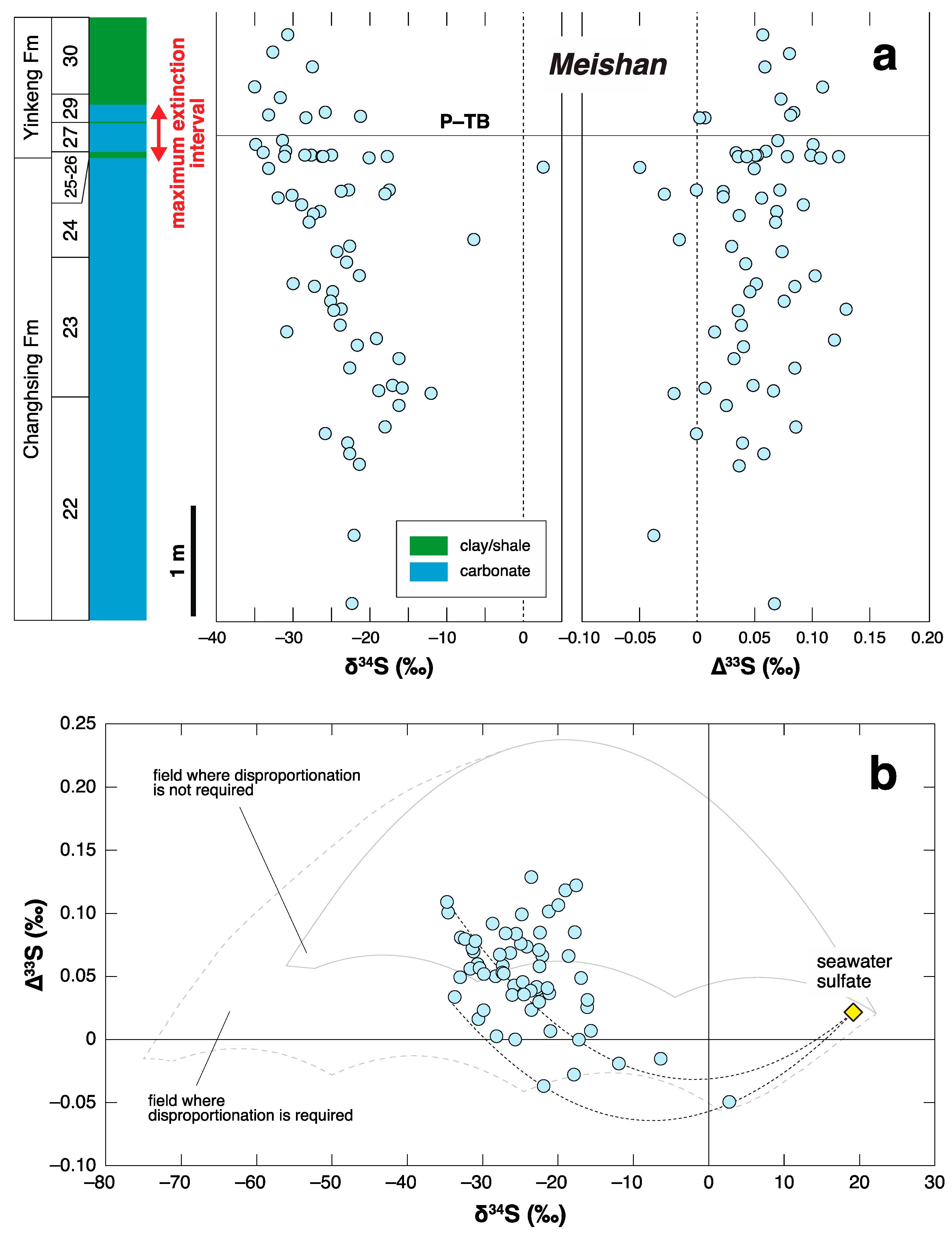
3.2. P-TB
3.3. S-SB
4. Negative ∆33S Signal as an Indicator of Shoaling?
5. Future Perspectives
5.1. Correlation between the Benthic Redox Conditions and ∆33S Records
5.2. SIMS Sulfur Isotope Record
5.3. Negative ∆33S Record during the Phanerozoic
Funding
Institutional Review Board Statement
Informed Consent Statement
Acknowledgments
Conflicts of Interest
References
- Alroy, J. The shifting balance of diversity among major marine animal groups. Science 2010, 329, 1191–1194. [Google Scholar] [CrossRef] [PubMed] [Green Version]
- Shen, S.Z.; Crowley, J.L.; Wang, Y.; Bowring, S.A.; Erwin, D.H.; Sadler, P.M.; Cao, C.Q.; Rothman, D.H.; Henderson, C.M.; Ramezani, J.; et al. Calibrating the End-Permian Mass Extinction. Science 2011, 334, 1367–1372. [Google Scholar] [CrossRef] [PubMed] [Green Version]
- Erwin, D.H. Extinction: How Life on Earth Nearly Ended 250 Million Years Ago, Updated ed.; Princeton Univ. Press: Princeton, NJ, USA, 2015; pp. 1–296. [Google Scholar]
- Yin, H.F.; Feng, Q.L.; Lai, X.L.; Baud, A.; Tong, J.N. The protracted Permo-Triassic crisis and multi-episode extinction around the Permian–Triassic boundary. Glob. Planet. Chang. 2007, 55, 1–20. [Google Scholar] [CrossRef]
- Isozaki, Y. Permo-Triassic boundary superanoxia and stratified superocean: Records from lost deep sea. Science 1997, 276, 235–238. [Google Scholar] [CrossRef] [PubMed]
- Isozaki, Y. Integrated ‘‘plume winter” scenario for the double-phased extinction during the Paleozoic–Mesozoic transition: The G-LB and P-TB events from a Panthalassan perspective. J. Asian Earth Sci. 2009, 36, 459–480. [Google Scholar] [CrossRef]
- Jin, Y.G.; Zhang, J.; Shang, Q.H. Two phases of the end-Permian mass extinction. In Pangea: Global Environments and Resources; Embry, A.F., Beauchamp, B., Glass, D.J., Eds.; Canadian Society of Petroleum Geologists: Calgary, AB, Canada, 1994; Volume 17, pp. 813–822. [Google Scholar]
- Stanley, S.M.; Yang, X. A double mass extinction at the end of the Paleozoic era. Science 1994, 266, 1340–1344. [Google Scholar] [CrossRef]
- Rampino, M.R.; Shen, S.Z. The end-Guadalupian (259.8 Ma) biodiversity crisis: The sixth major mass extinction? Hist. Biol. 2021, 33, 716–722. [Google Scholar] [CrossRef]
- Hallam, A. Why was there a delayed radiation after the end-Palaeozoic extinctions? Hist. Biol. 1991, 5, 257–262. [Google Scholar] [CrossRef]
- Galfetti, T.; Hochuli, P.A.; Brayard, A.; Bucher, H.; Weissert, H.; Vigran, J.O. Smithian-Spathian boundary event: Evidence for global climatic change in the wake of the end-Permian biotic crisis. Geology 2007, 35, 291–294. [Google Scholar] [CrossRef]
- Zhang, L.; Orchard, M.J.; Brayard, A.; Algeo, T.J.; Zhao, L.; Chen, Z.Q.; Lyu, Z. The Smithian/Spathian boundary (late Early Triassic): A review of ammonoid, conodont, and carbon-isotopic criteria. Earth-Sci. Rev. 2019, 195, 7–36. [Google Scholar] [CrossRef]
- Zhou, M.F.; Malpas, J.; Song, X.Y.; Robinson, P.T.; Sun, M.; Kennedy, A.K.; Lesher, C.M.; Keays, R.R. A temporal link between the Emeishan large igneous province (SW China) and the end-Guadalupian mass extinction. Earth Planet. Sci. Lett. 2002, 196, 113–122. [Google Scholar] [CrossRef]
- Wignall, P.B.; Sun, Y.D.; Bond, D.P.G.; Izon, G.; Newton, R.J.; Vedrine, S.; Widdowson, M.; Ali, J.R.; Lai, X.L.; Jiang, H.S.; et al. Volcanism, mass extinction, and carbon isotope fluctuations in the Middle Permian of China. Science 2009, 324, 1179–1182. [Google Scholar] [CrossRef]
- Isozaki, Y.; Kawahata, H.; Ota, A. A unique carbon isotope record across the Guadalupian–Lopingian (Middle–Upper Permian) boundary in mid-oceanic paleoatoll carbonates: The high-productivity “Kamura event” and its collapse in Panthalassa. Glob. Planet. Chang. 2007, 55, 21–38. [Google Scholar] [CrossRef]
- Saitoh, M.; Isozaki, Y.; Yao, J.X.; Ji, Z.S.; Ueno, Y.; Yoshida, N. The appearance of an oxygen-depleted condition on the Capitanian disphotic slope/basin in South China: Middle-upper Permian stratigraphy at Chaotian in northern Sichuan. Glob. Planet. Chang. 2013, 105, 180–192. [Google Scholar] [CrossRef]
- Saitoh, M.; Isozaki, Y.; Ueno, Y.; Yoshida, N.; Yao, J.X.; Ji, Z.S. Middle-Upper Permian carbon isotope stratigraphy at Chaotian, South China: Pre-extinction multiple upwelling of oxygen-depleted water onto continental shelf. J. Asian Earth Sci. 2013, 67–68, 51–62. [Google Scholar] [CrossRef]
- Yan, D.; Liqin, Z.; Zhen, Q. Carbon and sulfur isotopic fluctuations associated with the end-Guadalupian mass extinction in South China. Gondwana Res. 2013, 24, 1276–1282. [Google Scholar] [CrossRef]
- Becker, L.; Poreda, R.J.; Hunt, A.G.; Bunch, T.E.; Rampino, M. Impact event at the Permian–Triassic boundary: Evidence from extraterrestrial noble gases in fullerenes. Science 2001, 291, 1530–1533. [Google Scholar] [CrossRef] [Green Version]
- Renne, P.R.; Basu, A.R. Rapid eruption of the Siberian traps flood basalts at the Permian-Triassic boundary. Science 1991, 253, 176–179. [Google Scholar] [CrossRef] [PubMed] [Green Version]
- Reichow, M.K.; Pringle, M.S.; Al’Mukhamedov, A.I.; Allen, M.B.; Andreichev, V.L.; Buslov, M.M.; Davies, C.E.; Fedoseev, G.S.; Fitton, J.G.; Inger, S.; et al. The timing and extent of the eruption of the Siberian Traps large igneous province: Implications for the end-Permian environmental crisis. Earth Planet Sci. Lett. 2009, 277, 9–20. [Google Scholar] [CrossRef] [Green Version]
- Joachimski, M.M.; Lai, X.L.; Shen, S.Z.; Jiang, H.S.; Luo, G.M.; Chen, B.; Chen, J.; Sun, Y. Climate warming in the latest Permian and the Permian-Triassic mass extinction. Geology 2012, 40, 195–198. [Google Scholar] [CrossRef]
- Wignall, P.B.; Hallam, A. Anoxia as a cause of the Permian/Triassic mass extinction: Facies evidence from northern Italy and the western United States. Palaeogeogr. Palaeoclimatol. Palaeoecol. 1992, 93, 21–46. [Google Scholar] [CrossRef]
- Kump, L.R.; Pavlov, A.; Arthur, M.A. Massive release of hydrogen sulfide to the surface ocean and atmosphere during intervals of oceanic anoxia. Geology 2005, 33, 397–400. [Google Scholar] [CrossRef]
- Knoll, A.H.; Bambach, R.K.; Payne, J.L.; Pruss, S.; Fischer, W.W. Paleophysiology and end-Permian mass extinction. Earth Planet Sci. Lett. 2007, 256, 295–313. [Google Scholar] [CrossRef]
- Clarkson, M.O.; Kasemann, S.A.; Wood, R.A.; Lenton, T.M.; Daines, S.J.; Richoz, S.; Ohnemueller, F.; Meixner, A.; Poulton, S.W.; Tipper, E.T. Ocean acidification and the Permo-Triassic mass extinction. Science 2015, 348, 229–232. [Google Scholar] [CrossRef] [Green Version]
- Payne, J.L.; Kump, L.R. Evidence for recurrent Early Triassic massive volcanism from quantitative interpretation of carbon isotope fluctuations. Earth Planet. Sci. Lett. 2007, 256, 264–277. [Google Scholar] [CrossRef]
- Cui, Y.; Kump, L.R. Global warming and the end-Permian extinction event: Proxy and modeling perspectives. Earth-Sci. Rev. 2015, 149, 5–22. [Google Scholar] [CrossRef] [Green Version]
- Jurikova, H.; Gutjahr, M.; Wallmann, K.; Flögel, S.; Liebetrau, V.; Posenato, R.; Angiolini, L.; Garbelli, C.; Brand, U.; Wiedenbeck, M.; et al. Permian–Triassic mass extinction pulses driven by major marine carbon cycle perturbations. Nat. Geosci. 2020, 13, 745–750. [Google Scholar] [CrossRef]
- Wu, Y.Y.; Chu, D.L.; Tong, J.N.; Song, H.J.; Corso, J.D.; Wignall, P.B.; Song, H.Y.; Du, Y.; Cui, Y. Six-fold increase of atmospheric pCO2 during the Permian–Triassic mass extinction. Nat. Commun. 2021, 12, 2137. [Google Scholar] [CrossRef] [PubMed]
- Retallack, G.J.; Jahren, A.H. Methane release from igneous intrusion of coal during Late Permian extinction events. J. Geol. 2008, 116, 1–20. [Google Scholar] [CrossRef] [Green Version]
- Saitoh, M.; Isozaki, Y. Carbon isotope chemostratigraphy across the Permian-Triassic boundary at Chaotian, China: Implications for the global methane cycle in the aftermath of the extinction. Front. Earth Sci. 2021, 8, 596178. [Google Scholar] [CrossRef]
- Sun, Y.; Joachimski, M.M.; Wignall, P.B.; Yan, C.; Chen, Y.; Jiang, H.; Wang, L.; Lai, X.L. Lethally hot temperatures during the Early Triassic greenhouse. Science 2012, 338, 366–370. [Google Scholar] [CrossRef] [Green Version]
- Song, H.J.; Song, H.Y.; Tong, J.N.; Gordon, G.W.; Wignall, P.B.; Tian, L.; Zheng, W.; Algeo, T.J.; Liang, L.; Bai, R.Y.; et al. Conodont calcium isotopic evidence for multiple shelf acidification events during the Early Triassic. Chem. Geol. 2021, 562, 120038. [Google Scholar] [CrossRef]
- Grasby, S.E.; Beauchamp, B.; Embry, A.; Sanei, H. Recurrent Early Triassic ocean anoxia. Geology 2013, 41, 175–178. [Google Scholar] [CrossRef]
- Lau, K.V.; Maher, K.; Altiner, D.; Kelley, B.M.; Kump, L.R.; Lehrmann, D.J.; Silva-Tamayo, J.C.; Weaver, K.L.; Yu, M.; Payne, J.L. Marine anoxia and delayed Earth system recovery after the end-Permian extinction. Proc. Natl. Acad. Sci. USA 2016, 113, 2360–2365. [Google Scholar] [CrossRef] [PubMed] [Green Version]
- Zhang, F.F.; Romaniello, S.J.; Algeo, T.J.; Lau, K.V.; Clapham, M.E.; Richoz, S.; Herrmann, A.D.; Smith, H.; Horacek, M.; Anbar, A.D. Multiple episodes of extensive marine anoxia linked to global warming and continental weathering following the latest Permian mass extinction. Sci. Adv. 2018, 4, e1602921. [Google Scholar] [CrossRef] [Green Version]
- Brayard, A.; Bucher, H.; Escarguel, G.; Fluteau, F.; Bourquin, S.; Galfetti, T. The Early Triassic ammonoid recovery: Paleoclimatic significance of diversity gradients. Palaeogeogr. Palaeoclimatol. Palaeoecol. 2006, 239, 374–395. [Google Scholar] [CrossRef]
- Stanley, S.M. Evidence from ammonoids and conodonts for multiple Early Triassic mass extinctions. Proc. Natl. Acad. Sci. USA 2009, 106, 15264–15267. [Google Scholar] [CrossRef] [PubMed] [Green Version]
- Grasby, S.E.; Sanei, H.; Beauchamp, B.; Chen, Z.H. Mercury deposition through the Permo–Triassic Biotic Crisis. Chem. Geol. 2013, 351, 209–216. [Google Scholar] [CrossRef]
- Payne, J.L.; Lehrmann, D.J.; Wei, J.Y.; Orchard, M.J.; Schrag, D.P.; Knoll, A.H. Large perturbations of the carbon cycle during recovery from the end-Permian extinction. Science 2004, 305, 506–509. [Google Scholar] [CrossRef] [Green Version]
- Romano, C.; Goudemand, N.; Vennemann, T.W.; Ware, D.; Schneebeli-Hermann, E.; Hochuli, P.A.; Brühwiler, T.; Brinkmann, W.; Bucher, H. Climatic and biotic upheavals following the end-Permian mass extinction. Nat. Geosci. 2013, 6, 57–60. [Google Scholar] [CrossRef]
- Song, H.Y.; Du, Y.; Algeo, T.J.; Tong, J.N.; Owens, J.D.; Song, H.J.; Tian, L.; Qiu, H.; Zhu, Y.Y.; Lyons, T.W. Cooling-driven oceanic anoxia across the Smithian/Spathian boundary (mid-Early Triassic). Earth-Sci. Rev. 2019, 195, 133–146. [Google Scholar] [CrossRef]
- Payne, J.L.; Clapham, M.E. End-Permian mass extinction in the oceans: An ancient analog for the twenty-first century? Ann. Rev. Earth Planet. Sci. 2012, 40, 89–111. [Google Scholar] [CrossRef] [Green Version]
- Farquhar, J.; Wing, B.A. Multiple sulfur isotopes and the evolution of the atmosphere. Earth Planet. Sci. Lett. 2003, 213, 1–13. [Google Scholar] [CrossRef]
- Johnston, D.T. Multiple sulfur isotopes and the evolution of Earth’s surface sulfur cycle. Earth-Sci. Rev. 2011, 106, 161–183. [Google Scholar] [CrossRef]
- Ovtcharova, M.; Bucher, H.; Schaltegger, U.; Galfetti, T.; Brayard, A.; Guex, J. New Early to Middle Triassic U–Pb ages from South China: Calibration with ammonoid biochronozones and implications for the timing of the Triassic biotic recovery. Earth Planet. Sci. Lett. 2006, 243, 463–475. [Google Scholar] [CrossRef]
- Gradstein, F.M.; Ogg, J.G.; Schmitz, M.D.; Ogg, G.M. Geologic Time Scale 2020; Elsevier: Amsterdam, The Netherlands, 2020; pp. 1–1357. [Google Scholar]
- Muttoni, G.; Gaetani, M.; Kent, D.V.; Sciunnach, D.; Angiolini, L.; Berra, F.; Garzanti, E.; Mattei, M.; Zanchi, A. Opening of the Neo-Tethys Ocean and the Pangea B to Pangea A transformation during the Permian. GeoArabia 2009, 14, 17–48. [Google Scholar] [CrossRef] [Green Version]
- Ono, S.; Wing, B.; Johnston, D.; Farquhar, J.; Rumble, D. Mass-dependent fractionation of quadruple stable sulfur isotope system as a new tracer of sulfur biogeochemical cycles. Geochim. Cosmochim. Acta 2006, 70, 2238–2252. [Google Scholar] [CrossRef]
- Farquhar, J.; Bao, H.M.; Thiemens, M. Atmospheric influence of Earth’s earliest sulfur cycle. Science 2000, 289, 756–758. [Google Scholar] [CrossRef] [Green Version]
- Ono, S. Photochemistry of sulfur dioxide and the origin of mass-independent isotope fractionation in Earth’s atmosphere. Ann. Rev. Earth Planet. Sci. 2017, 45, 301–329. [Google Scholar] [CrossRef]
- Johnston, D.T.; Wing, B.A.; Farquhar, J.; Kaufman, A.J.; Strauss, H.; Lyons, T.W.; Kah, L.C.; Canfield, D.E. Active Microbial Sulfur Disproportionation in the Mesoproterozoic. Science 2005, 310, 1477–1479. [Google Scholar] [CrossRef] [PubMed] [Green Version]
- Sim, M.S.; Bosak, T.; Ono, S. Large sulfur isotope fractionation does not require disproportionation. Science 2011, 333, 74–77. [Google Scholar] [CrossRef]
- Shen, Y.; Farquhar, J.; Zhang, H.; Masterson, A.; Zhang, T.G.; Wing, B.A. Multiple S-isotopic evidence for episodic shoaling of anoxic water during Late Permian mass extinction. Nature Commun. 2011, 2, 210. [Google Scholar] [CrossRef] [PubMed]
- Yin, H.F.; Zhang, K.; Tong, J.N.; Yang, Z.Y.; Wu, S.B. The Global Stratotype Section and Point (GSSP) of the Permian-Triassic Boundary. Episodes 2001, 24, 102–114. [Google Scholar]
- Jin, Y.G.; Wang, Y.; Wang, W.; Shang, Q.H.; Cao, C.Q.; Erwin, D.H. Pattern of marine mass extinction near the Permian-Triassic boundary in South China. Science 2000, 289, 432–436. [Google Scholar] [CrossRef] [PubMed]
- Wignall, P.B.; Hallam, A. Griesbachian (Earliest Triassic) palaeoenvironmental changes in the Salt Range, Pakistan and southeast China and their bearing on the Permo-Triassic mass extinction. Palaeogeogr. Palaeoclimatol. Palaeoecol. 1993, 102, 215–237. [Google Scholar] [CrossRef]
- Yin, H.F.; Jiang, H.S.; Xia, W.C.; Feng, Q.L.; Zhang, N.; Shen, J. The end-Permian regression in South China and its implication on mass extinction. Earth-Sci. Rev. 2014, 137, 19–33. [Google Scholar] [CrossRef]
- Baud, A.; Magaritz, M.; Holser, W.T. Permian–Triassic of the Tethys: Carbon isotope studies. Geol. Rundsch. 1989, 78, 649–677. [Google Scholar] [CrossRef]
- Grice, K.; Cao, C.Q.; Love, G.D.; Böttcher, M.E.; Twitchett, R.J.; Grosjean, E.; Summons, R.E.; Turgeon, S.C.; Dunning, W.; Jin, Y.G. Photic zone euxinia during the Permian-Triassic superanoxic event. Science 2005, 307, 706–709. [Google Scholar] [CrossRef] [PubMed] [Green Version]
- Li, G.S.; Wang, Y.B.; Shi, G.R.; Liao, W.; Yu, L. Fluctuations of redox conditions across the Permian–Triassic boundary—New evidence from the GSSP section in Meishan of South China. Palaeogeogr. Palaeoclimatol. Palaeoecol. 2016, 448, 48–58. [Google Scholar] [CrossRef]
- Hinojosa, J.L.; Brown, S.T.; Chen, J.; DePaolo, D.J.; Paytan, A.; Shen, S.Z.; Payne, J.L. Evidence for end-Permian ocean acidification from calcium isotopes in biogenic apatite. Geology 2012, 40, 743–746. [Google Scholar] [CrossRef]
- Grasby, S.E.; Shen, W.J.; Yin, R.S.; Gleason, J.D.; Blum, J.D.; Lepak, R.F.; Hurley, J.P.; Beauchamp, B. Isotopic signatures of mercury contamination in latest Permian oceans. Geology 2017, 45, 55–58. [Google Scholar] [CrossRef]
- Song, H.J.; Wignall, P.B.; Tong, J.N.; Yin, H.F. Two pulses of extinction during the Permian–Triassic crisis. Nat. Geosci. 2013, 6, 52–56. [Google Scholar] [CrossRef]
- Yin, H.F.; Xie, S.C.; Luo, G.M.; Algeo, T.J.; Zhang, K. Two episodes of environmental change at the Permian–Triassic boundary of the GSSP section Meishan. Earth-Sci. Rev. 2012, 115, 163–172. [Google Scholar] [CrossRef]
- Zhang, G.J.; Zhang, X.L.; Hu, D.P.; Li, D.D.; Algeo, T.J.; Farquhar, J.; Henderson, C.M.; Qin, L.P.; Shen, M.; Shen, D.; et al. Redox chemistry changes in the Panthalassic Ocean linked to the end-Permian mass extinction and delayed Early Triassic biotic recovery. Proc. Natl. Acad. Sci. USA 2017, 114, 1806–1810. [Google Scholar] [CrossRef] [Green Version]
- Wu, N.P.; Farquhar, J.; Strauss, H.; Kim, S.T.; Canfield, D.E. Evaluating the S-isotope fractionation associated with Phanerozoic pyrite burial. Geochim. Cosmochim. Acta 2010, 74, 2053–2071. [Google Scholar] [CrossRef]
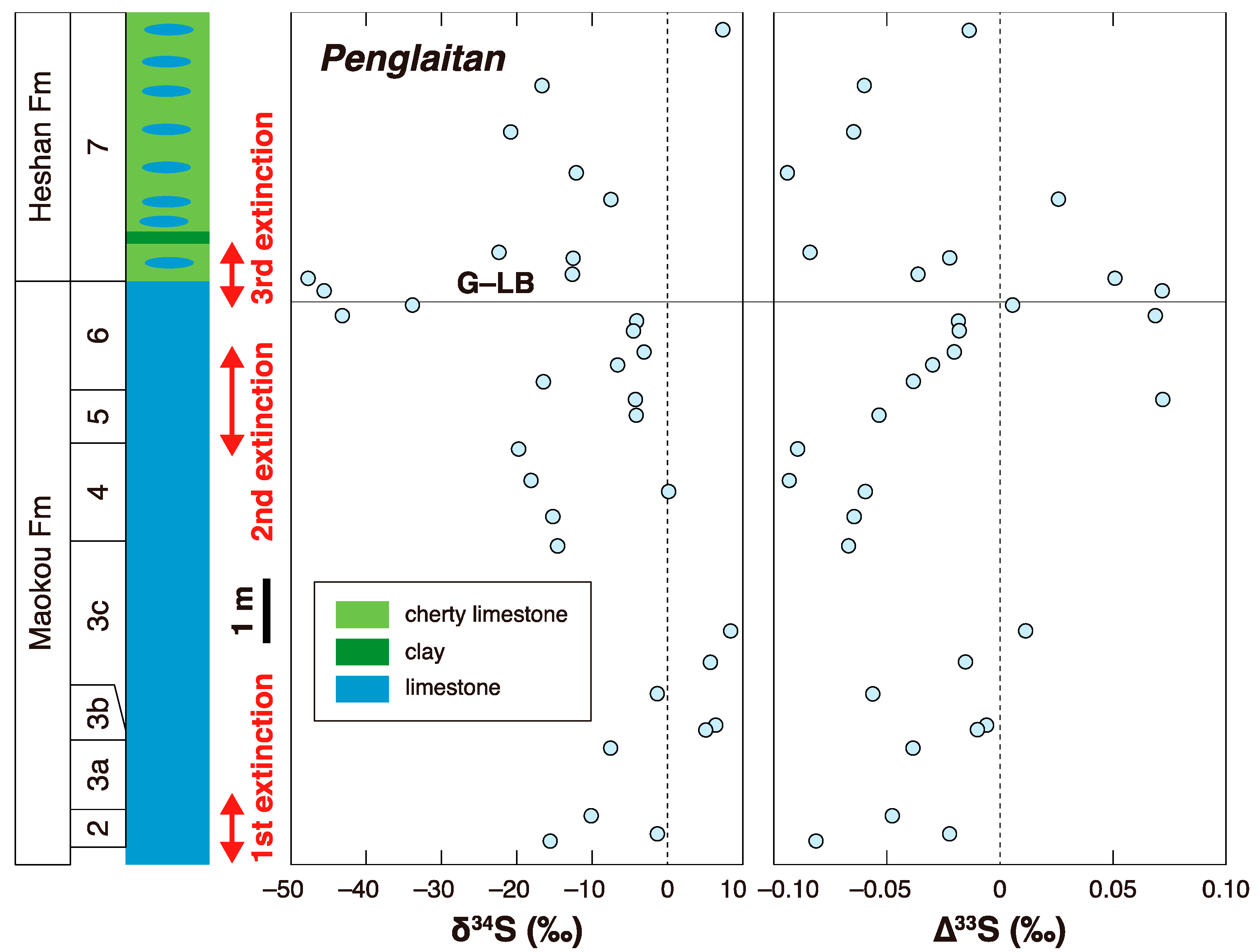
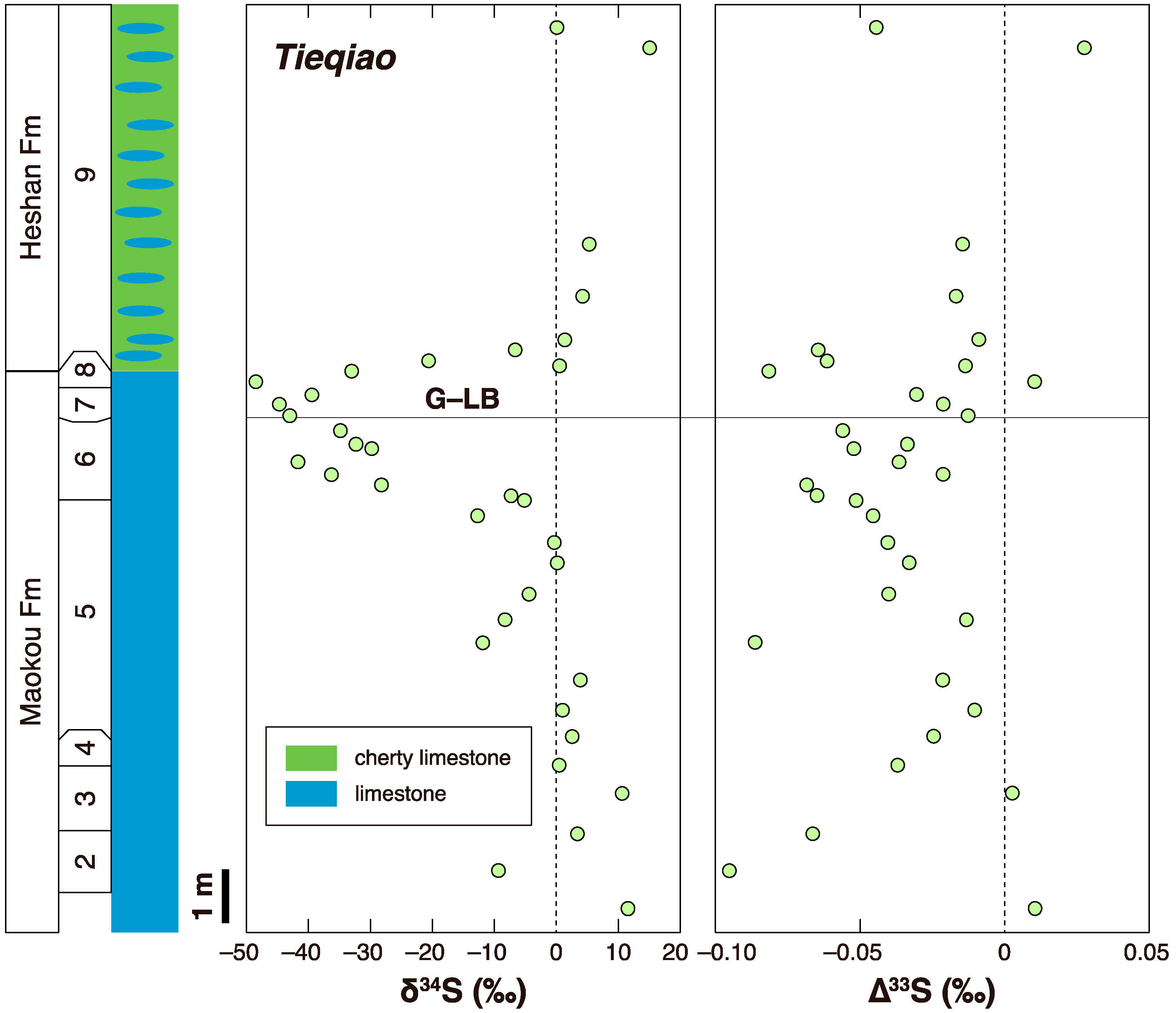
- Zhang, G.J.; Zhang, X.L.; Li, D.D.; Farquhar, J.; Shen, S.Z.; Chen, X.Y.; Shen, Y. Widespread shoaling of sulfidic waters linked to the end-Guadalupian (Permian) mass extinction. Geology 2015, 43, 1091–1094. [Google Scholar] [CrossRef]
- Jin, Y.G.; Mei, S.L.; Wang, W.; Wang, X.D.; Shen, S.Z.; Shang, Q.H.; Chen, Z.Q. On the Lopingian Series of the Permian system. In Permian Stratigraphy, Environments and Resources; Jin, Y.G., Wardlaw, B.R., Wang, Y., Eds.; China University of Science and Technology Press: Hefei, China, 1998; Volume 9, pp. 1–18. [Google Scholar]
- Jin, Y.G.; Shen, S.Z.; Henderson, C.M.; Wang, X.D.; Wang, W.; Wang, Y.; Cao, C.Q.; Shang, Q.H. The Global Stratotype Section and Point (GSSP) for the boundary between the Capitanian and Wuchiapingian Stage (Permian). Episodes 2006, 29, 253–262. [Google Scholar] [CrossRef] [Green Version]
- Shen, S.Z.; Wang, Y.; Henderson, C.M.; Cao, C.Q.; Wang, W. Biostratigraphy and lithofacies of the Permian System in the Laibin–Heshan area of Guangxi, South China. Palaeoworld 2007, 16, 120–139. [Google Scholar] [CrossRef]
- Qiu, Z.; Wang, Q.C.; Zou, C.N.; Yan, D.; Wei, H.Y. Transgressive–regressive sequences on the slope of an isolated carbonate platform (Middle–Late Permian, Laibin, South China). Facies 2014, 60, 327–345. [Google Scholar] [CrossRef]
- Wei, H.Y.; Wei, X.M.; Qiu, Z.; Song, H.Y.; Shi, G. Redox conditions across the G–L boundary in South China: Evidence from pyrite morphology and sulfur isotopic compositions. Chem. Geol. 2016, 440, 1–14. [Google Scholar] [CrossRef]
- Wignall, P.B.; Védrine, S.; Bond, D.P.G.; Wang, W.; Lai, X.L.; Ali, J.R.; Jiang, H.S. Facies analysis and sea-level change at the Guadalupian–Lopingian Global Stratotype (Laibin, South China), and its bearing on the end-Guadalupian mass extinction. J. Geol. Soc. 2009, 166, 655–666. [Google Scholar] [CrossRef]
- Ehiro, M.; Shen, S.Z. Permian ammonoid Kufengoceras from the uppermost Maokou Formation (earliest Wuchiapingian) at Penglaitan, Laibin Area, Guangxi Autonomous Region, South China. Paleontol. Res. 2008, 12, 255–259. [Google Scholar] [CrossRef]
- Ehiro, M.; Shen, S.Z. Ammonoid succession across the Wuchiapingian/Changhsingian boundary of the northern Penglaitan Section in the Laibin area, Guangxi, South China. Geol. J. 2010, 45, 162–169. [Google Scholar] [CrossRef]
- Kaiho, K.; Chen, Z.Q.; Ohashi, T.; Arinobu, T.; Sawada, K.; Cramer, B.S. A negative carbon isotope anomaly associated with the earliest Lopingian (Late Permian) mass extinction. Palaeogeogr. Palaeoclimatol. Palaeoecol. 2005, 223, 172–180. [Google Scholar] [CrossRef]
- Shen, S.Z.; Shi, G.R. Latest Guadalupian brachiopods from the Guadalupian/Lopingian boundary GSSP section at Penglaitan in Laibin, Guangxi, South China and implications for the timing of the pre-Lopingian crisis. Palaeoworld 2009, 18, 152–161. [Google Scholar] [CrossRef]
- Huang, Y.G.; Chen, Z.Q.; Wignall, P.B.; Grasby, S.E.; Zhao, L.S.; Wang, X.D.; Kaiho, K. Biotic responses to volatile volcanism and environmental stresses over the Guadalupian-Lopingian (Permian) transition. Geology 2019, 47, 175–178. [Google Scholar] [CrossRef]
- Yang, X.N.; Liu, J.R.; Shi, G.J. Extinction process and patterns of Middle Permian Fusulinaceans in southwest China. Lethaia 2004, 37, 139–147. [Google Scholar] [CrossRef]
- Clapham, M.E.; Shen, S.Z.; Bottjer, D.J. The double mass extinction revisited: Reassessing the severity, selectivity, and causes of the end-Guadalupian biotic crisis (Late Permian). Paleobiology 2009, 35, 32–50. [Google Scholar] [CrossRef]
- Groves, J.R.; Wang, Y. Timing and Size Selectivity of the Guadalupian (Middle Permian) Fusulinoidean Extinction. J. Paleontol. 2013, 87, 183–196. [Google Scholar] [CrossRef]
- Arefifard, S.; Payne, J.L. End-Guadalupian extinction of larger fusulinids in central Iran and implications for the global biotic crisis. Palaeogeogr. Palaeoclimatol. Palaeoecol. 2020, 550, 109743. [Google Scholar] [CrossRef]
- Bond, D.P.G.; Wignall, P.B.; Wang, W.; Izon, G.; Jiang, H.S.; Lai, X.L.; Sun, Y.D.; Newton, R.J.; Shao, L.Y.; Védrine, S.; et al. The mid-Capitanian (Middle Permian) mass extinction and carbon isotope record of South China. Palaeogeogr. Palaeoclimatol. Palaeoecol. 2010, 292, 282–294. [Google Scholar] [CrossRef]
- Bond, D.P.G.; Hilton, J.; Wignall, P.B.; Ali, J.R.; Stevens, L.G.; Sun, Y.D.; Lai, X.L. The Middle Permian (Capitanian) mass extinction on land and in the oceans. Earth-Sci. Rev. 2010, 102, 100–116. [Google Scholar] [CrossRef]
- Zhang, B.; Yao, S.; Wignall, P.B.; Hu, W.X.; Liu, B.; Ren, Y. New timing and geochemical constraints on the Capitanian (Middle Permian) extinction and environmental changes in deep-water settings: Evidence from the Lower Yangtze region of South China. J. Geol. Soc. 2019, 176, 588–608. [Google Scholar] [CrossRef]
- Sun, Y.D.; Liu, X.T.; Yan, J.X.; Li, B.; Chen, B.; Bond, D.P.G.; Joachimski, M.M.; Wignall, P.B.; Wang, X.; Lai, X.L. Permian (Artinskian to Wuchapingian) conodont biostratigraphy in the Tieqiao section, Laibin area, South China. Palaeogeogr. Palaeoclimatol. Palaeoecol. 2017, 465, 42–63. [Google Scholar] [CrossRef]
- Chen, Z.Q.; George, A.D.; Yang, W.R. Effects of Middle–Late Permian sea-level changes and mass extinction on the formation of the Tieqiao skeletal mound in the Laibin area, South China. Aus. J. Earth Sci. 2009, 56, 745–763. [Google Scholar] [CrossRef]
- Zhang, Z.; Wang, Y.; Zheng, Q.F. Middle Permian smaller foraminifers from the Maokou Formation at the Tieqiao section, Guangxi, South China. Palaeoworld 2015, 24, 263–276. [Google Scholar] [CrossRef]
- Wardlaw, B.R.; Nestell, M.K. Latest Middle Permian conodonts from the Apache Mountains, West Texas. Micropaleontology 2010, 56, 149–184. [Google Scholar] [CrossRef]
- Kennedy, W. Geology of Part of the Northwestern Apache Mountains, Southeast Culberson County, West Texas, U.S.A. Master’s Thesis, The Univiversity of Texas Arlington, Arlington, TX, USA, 2009. [Google Scholar]
- Haq, B.U.; Schutter, S.R. A chronology of Paleozoic sea-level changes. Science 2008, 322, 64–68. [Google Scholar] [CrossRef]
- Shen, S.Z.; Yuan, D.X.; Henderson, C.M.; Wu, Q.; Zhang, Y.C.; Zhang, H.; Mu, L.; Ramezani, J.; Wang, X.D.; Lambert, L.L.; et al. Progress, problems and prospects: An overview of the Guadalupian Series of South China and North America. Earth-Sci. Rev. 2020, 211, 103412. [Google Scholar] [CrossRef]
- Nestell, G.P.; Nestell, M.K. Late Capitanian (latest Guadalupian, Middle Permian) radiolarians from the Apache Mountains, West Texas. Micropaleontology 2010, 56, 7–68. [Google Scholar] [CrossRef]
- Lambert, L.L.; Wardlaw, B.R.; Nestell, M.K.; Nestell, G.P. Latest Guadalupian (Middle Permian) conodonts and foraminifers from West Texas. Micropaleontology 2002, 48, 343–364. [Google Scholar] [CrossRef] [Green Version]
- Henderson, C.M. Permian conodont biostratigraphy. In The Permian Timescale; Lucas, S.G., Shen, S.Z., Eds.; Geological Society: London, UK, 2018; Volume 450, pp. 119–142. [Google Scholar]
- Wu, Q.; Ramezani, J.; Zhang, H.; Yuan, D.X.; Erwin, D.H.; Henderson, C.M.; Lambert, L.L.; Zhang, Y.C.; Shen, S.Z. High-precision U-Pb zircon age constraints on the Guadalupian in West Texas, USA. Palaeogeogr. Palaeoclimatol. Palaeoecol. 2020, 548, 109668. [Google Scholar] [CrossRef]
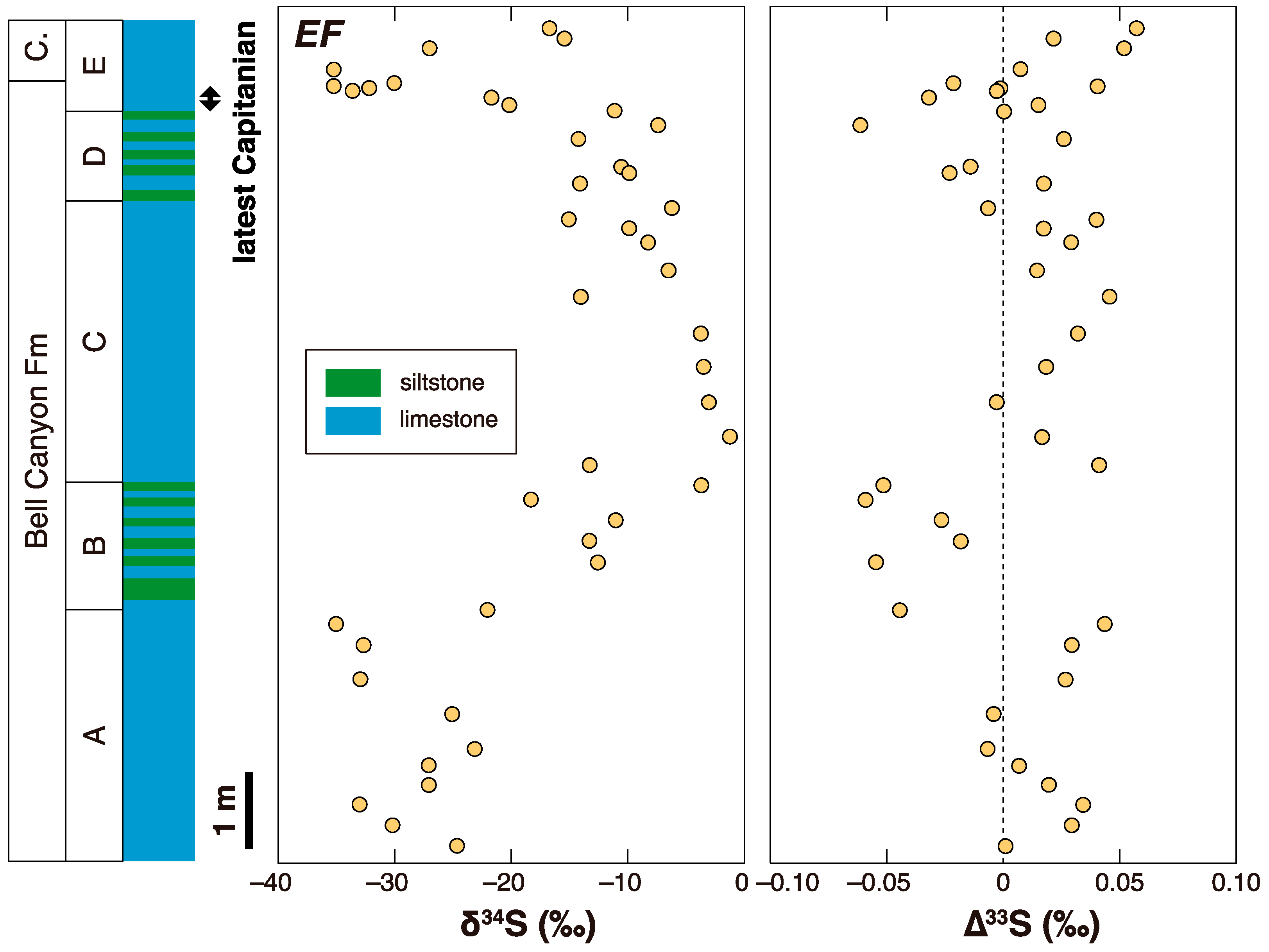
- Smith, B.P.; Larson, T.; Martindale, R.C.; Kerans, C. Impacts of basin restriction on geochemistry and extinction patterns: A case from the Guadalupian Delaware Basin, USA. Earth Planet. Sci. Lett. 2020, 530, 115876. [Google Scholar] [CrossRef]
- Saitoh, M.; Ueno, Y.; Matsu’ura, F.; Kawamura, T.; Isozaki, Y.; Yao, J.Y.; Ji, Z.S.; Yoshida, N. Multiple sulfur isotope records at the end-Guadalupian (Permian) at Chaotian, China: Implications for a role of bioturbation in the Phanerozoic sulfur cycle. J. Asian Earth Sci. 2017, 135, 70–79. [Google Scholar] [CrossRef]
- Saitoh, M.; Ueno, Y.; Isozaki, Y.; Nishizawa, M.; Shozugawa, K.; Kawamura, T.; Yao, J.X.; Ji, Z.S.; Takai, K.; Yoshida, N.; et al. Isotopic evidence for water-column denitrification and sulfate reduction at the end-Guadalupian (Middle Permian). Glob. Planet. Chang. 2014, 123, 110–120. [Google Scholar] [CrossRef]
- Isozaki, Y.; Yao, J.X.; Ji, Z.S.; Saitoh, M.; Kobayashi, N.; Sakai, H. Rapid sea-level change in the Late Guadalupian (Permian) on the Tethyan side of South China: Litho- and biostratigraphy of the Chaotian section in Sichuan. Proc. Jpn. Acad. Ser. B 2008, 84, 344–353. [Google Scholar] [CrossRef] [PubMed] [Green Version]
- Lai, X.L.; Wang, W.; Wignall, P.B.; Bond, D.P.G.; Jiang, H.S.; Ali, J.R.; John, E.H.; Sun, Y.D. Palaeoenvironmental change during the end-Guadalupian (Permian) mass extinction in Sichuan, China. Palaeogeogr. Palaeoclimatol. Palaeoecol. 2008, 269, 78–93. [Google Scholar] [CrossRef]
- Schoepfer, S.D.; Henderson, C.M.; Garrison, G.H.; Foriel, J.; Ward, P.D.; Selby, D.; Hower, J.C.; Algeo, T.J.; Shen, Y.N. Termination of a continent-margin upwelling system at the Permian–Triassic boundary (Opal Creek, Alberta, Canada). Glob. Planet. Chang. 2013, 105, 21–35. [Google Scholar] [CrossRef] [Green Version]
- Schoepfer, S.D.; Henderson, C.M.; Garrison, G.H.; Ward, P.D. Cessation of a productive coastal upwelling system in the Panthalassic Ocean at the Permian–Triassic boundary. Palaeogeogr. Palaeoclimatol. Palaeoecol. 2012, 313–314, 181–188. [Google Scholar] [CrossRef]
- Kenig, F.; Hudson, J.D.; Sinninghe Damste, J.S.; Popp, B.N. Intermittent euxinia: Reconciliation of a Jurassic black shale with its biofacies. Geology 2004, 32, 421–424. [Google Scholar] [CrossRef]
- Algeo, T.J.; Kuwahara, K.; Sano, H.; Bates, S.; Lyons, T.; Elswick, E.; Hinnov, L.; Ellwood, B.; Moser, J.; Maynard, J.B. Spatial variation in sediment fluxes, redox conditions, and productivity in the Permian–Triassic Panthalassic Ocean. Palaeogeogr. Palaeoclimatol. Palaeoecol. 2011, 308, 65–83. [Google Scholar] [CrossRef]
- Fujisaki, W.; Sawaki, Y.; Matsui, Y.; Yamamoto, S.; Isozaki, Y.; Maruyama, S. Redox condition and nitrogen cycle in the Permian deep mid-ocean: A possible contrast between Panthalassa and Tethys. Glob. Planet. Chang. 2019, 172, 179–199. [Google Scholar] [CrossRef]
- Kuwahara, K.; Nakae, S.; Yao, A. Late Permian “Toishi-type” siliceous mudstone in the Mino-Tamba Belt. J. Geol. Soc. Japan 1991, 97, 1005–1008, In Japanese with English abstract. [Google Scholar] [CrossRef] [Green Version]
- Kuwahara, K.; Yao, A. Late Permian radiolarian faunal change in bedded chert of the Mino Belt, Japan. New Osaka Micropaleontol. 2001, 12, 33–49, In Japanese with English abstract. [Google Scholar]
- Yao, J.X.; Yao, A.; Kuwahara, K. Upper Permian biostratigraphic correlation between conodont and radiolarian zones in the Tamba-Mino Terrane, Southwest Japan. J. Geosci. Osaka City Univ. 2001, 44, 97–119. [Google Scholar]
- Takahashi, S.; Yamakita, S.; Suzuki, N.; Kaiho, K.; Ehiro, M. High organic carbon content and a decrease in radiolarians at the end of the Permian in a newly discovered continuous pelagic section: A coincidence? Palaeogeogr. Palaeoclimatol. Palaeoecol. 2009, 271, 1–12. [Google Scholar] [CrossRef]
- Kaiho, K.; Oba, M.; Fukuda, Y.; Ito, K.; Ariyoshi, S.; Gorjan, P.; Riu, Y.; Takahashi, S.; Chen, Z.Q.; Tong, J.N.; et al. Changes in depth-transect redox conditions spanning the end-Permian mass extinction and their impact on the marine extinction: Evidence from biomarkers and sulfur isotopes. Glob. Planet. Chang. 2012, 94-95, 20–32. [Google Scholar] [CrossRef]
- Sugiyama, K. Lower and Middle Triassic radiolarians from Mt. Kinkazan, Gifu Prefecture, central Japan. Trans. Proc. Palaeontol. Soc. Jpn. 1992, 167, 1180–1223. [Google Scholar]
- Takemura, A.; Sakai, M.; Sakamoto, S.; Aono, R.; Takemura, S.; Yamakita, S. Earliest Triassic radiolarians from the ARH and ARF sections on Arrow Rocks, Waipapa Terrane, Northland, New Zealand. In The Oceanic Permian/Triassic Boundary Sequence at Arrow Rocks (Oruatemanu) Northland, New Zealand; Sporli, K.B., Takemura, A., Hori, R.S., Eds.; GNS Science Monography: Lower Hutt, New Zealand, 2007; Volume 24, pp. 97–107. [Google Scholar]
- Algeo, T.J.; Hinnov, L.; Moser, J.; Maynard, J.B.; Elswick, E.; Kuwahara, K.; Sano, H. Changes in productivity and redox conditions in the Panthalassic Ocean during the latest Permian. Geology 2010, 38, 187–190. [Google Scholar] [CrossRef]
- Yamakita, S.; Kadota, N.; Kato, T.; Tada, R.; Ogihara, S.; Tajika, E.; Hamada, Y. Confirmation of the Permian/Triassic boundary in deep-sea sedimentary rocks; earliest Triassic conodonts from black carbonaceous claystone of the Ubara section in the Tamba Belt, Southwest Japan. J. Geol. Soc. Jpn. 1999, 105, 895–898. [Google Scholar] [CrossRef] [Green Version]
- Isozaki, Y. Superanoxia Across the Permo-Triassic Boundary: Record in Accreted Deep-Sea Pelagic Chert in Japan. In Pangea: Global Environments and Resources; Embry, A.F., Beauchamp, B., Glass, D.J., Eds.; Canadian Society of Petroleum Geologists: Calgary, AB, Canada, 1994; Volume 17, pp. 805–812. [Google Scholar]
- Kakuwa, Y. Evaluation of palaeo-oxygenation of the ocean bottom across the Permian–Triassic boundary. Glob. Planet. Chang. 2008, 63, 40–56. [Google Scholar] [CrossRef]
- Takahashi, S.; Yamasaki, S.; Ogawa, Y.; Kimura, K.; Kaiho, K.; Yoshida, T.; Tsuchiya, N. Bioessential element-depleted ocean following the euxinic maximum of the end-Permian mass extinction. Earth Planet. Sci. Lett. 2014, 393, 94–104. [Google Scholar] [CrossRef]
- Grasby, S.E.; Bond, D.P.G.; Wignall, P.B.; Yin, R.; Strachan, L.J.; Takahashi, S. Transient Permian-Triassic euxinia in the southern Panthalassa deep ocean. Geology 2021, 49, 889–893. [Google Scholar] [CrossRef]
- Saitoh, M.; Ueno, Y.; Isozaki, Y.; Yoshida, N. Multiple sulfur isotope chemostratigraphy across the Permian–Triassic boundary at Chaotian, China: Implications for a shoaling model of toxic deep-waters. Isl. Arc 2021, 30, e12398. [Google Scholar] [CrossRef]
- Isozaki, Y.; Shimizu, N.; Yao, J.X.; Ji, Z.S.; Matsuda, T. End-Permian extinction and volcanism-induced environmental stress: The Permian–Triassic boundary interval of lower-slope facies at Chaotian, South China. Palaeogeogr. Palaeoclimatol. Palaeoecol. 2007, 252, 218–238. [Google Scholar] [CrossRef]
- Saitoh, M.; Ueno, Y.; Nishizawa, M.; Isozaki, Y.; Takai, K.; Yao, J.X.; Ji, Z.S. Nitrogen isotope chemostratigraphy across the Permian-Triassic boundary at Chaotian, Sichuan, south China. J. Asian Earth Sci. 2014, 93, 113–128. [Google Scholar] [CrossRef]
- Thomazo, C.; Brayard, A.; Elmeknassi, S.; Vennin, E.; Olivier, N.; Caravaca, G.; Escarguel, G.; Fara, E.; Bylund, K.G.; Jenks, J.F.; et al. Multiple sulfur isotope signals associated with the late Smithian event and the Smithian/Spathian boundary. Earth-Sci. Rev. 2019, 195, 96–113. [Google Scholar] [CrossRef]
- Vennin, E.; Olivier, N.; Brayard, A.; Bour, I.; Thomazo, C.; Escarguel, G.; Fara, E.; Bylund, K.G.; Jenks, J.F.; Stephen, D.A.; et al. Microbial deposits in the aftermath of the end-Permian mass extinction: A diverging case from the Mineral Mountains (Utah, USA). Sedimentology 2015, 62, 753–792. [Google Scholar] [CrossRef]
- Brayard, A.; Bylund, K.G.; Jenks, J.F.; Stephen, D.A.; Olivier, N.; Escarguel, G.; Fara, E.; Vennin, E. Smithian ammonoid faunas from Utah: Implications for Early Triassic biostratigraphy, correlation and basinal paleogeography. Swiss J. Palaeontol. 2013, 132, 141–219. [Google Scholar] [CrossRef]
- Thomazo, C.; Vennin, E.; Brayard, A.; Bour, I.; Mathieu, O.; Elmeknassi, S.; Olivier, N.; Escarguel, G.; Bylund, K.G.; Jenks, J.; et al. A diagenetic control on the Early Triassic Smithian-Spathian carbon isotopic excursions recorded in the marine settings of the Thaynes Group (Utah, USA). Geobiology 2016, 14, 220–236. [Google Scholar] [CrossRef]
- Clarkson, M.O.; Wood, R.A.; Poulton, S.W.; Richoz, S.; Newton, R.J.; Kasemann, S.A.; Bowyer, F.; Krystyn, L. Dynamic anoxic ferruginous conditions during the end-Permian mass extinction and recovery. Nature Commun. 2016, 7, 12236. [Google Scholar] [CrossRef]
- Whitehouse, M.J. Multiple sulfur isotope determination by SIMS: Evaluation of reference sulfides for ∆33S with observations and a case study on the determination of ∆36S. Geostand. Geoanal. Res. 2013, 37, 19–33. [Google Scholar] [CrossRef]
- Marin-Carbonne, J.; Rollion-Bard, C.; Bekker, A.; Rouxel, O.; Agangi, A.; Cavalazzi, B.; Wohlgemuth-Ueberwasser, C.C.; Hofmann, A.; McKeegan, K.D. Coupled Fe and S isotope variations in pyrite nodules from Archean shale. Earth Planet. Sci. Lett. 2014, 392, 67–79. [Google Scholar] [CrossRef] [Green Version]
- Ushikubo, T.; Williford, K.H.; Farquhar, J.; Johnston, D.T.; Van Kranendonk, M.J.; Valley, J.W. Development of in situ sulfur four-isotope analysis with multiple Faraday cup detectors by SIMS and application to pyrite grains in a Paleoproterozoic glaciogenic sandstone. Chem. Geol. 2014, 383, 86–99. [Google Scholar] [CrossRef]
- Harazim, D.; Virtasalo, J.J.; Denommee, K.C.; Thiemeyer, N.; Lahaye, Y.; Whitehouse, M.J. Exceptional sulfur and iron isotope enrichment in millimetre-sized, early Palaeozoic animal burrows. Sci. Rep. 2020, 10, 20270. [Google Scholar] [CrossRef]
- Wang, W.; Hu, Y.L.; Muscente, A.D.; Cui, H.; Guan, C.G.; Hao, J.L.; Zhou, C.M. Revisiting Ediacaran sulfur isotope chemostratigraphy with in situ nanoSIMS analysis of sedimentary pyrite. Geology 2021, 49, 611–616. [Google Scholar] [CrossRef]
- Nabhan, S.; Wiedenbeck, M.; Milke, R.; Heubeck, C. Biogenic overgrowth on detrital pyrite in ca. 3.2 Ga Archean paleosols. Geology 2016, 44, 763–766. [Google Scholar] [CrossRef]
- Li, D.D.; Zhang, X.L.; Hu, D.P.; Li, D.; Zhang, G.J.; Zhang, X.; Ling, H.F.; Xu, Y.; Shen, Y. Multiple S-isotopic constraints on paleo-redox and sulfate concentrations across the Ediacaran-Cambrian transition in South China. Precambrian Res. 2020, 349, 105500. [Google Scholar] [CrossRef]
- Chen, K.; Hu, D.P.; Zhang, X.L.; Zhu, H.; Sun, L.; Li, M.; Shen, Y. Minor Δ33S anomalies coincide with biotic turnover events during the Great Ordovician Biodiversification Event (GOBE) in South China. Glob. Planet. Chang. 2020, 184, 103069. [Google Scholar] [CrossRef]
- Luo, G.M.; Richoz, S.; van de Schootbrugge, B.; Algeo, T.J.; Xie, S.C.; Ono, S.; Summons, R.E. Multiple sulfur-isotopic evidence for a shallowly stratified ocean following the Triassic-Jurassic boundary mass extinction. Geochim. Cosmochim. Acta 2018, 231, 73–87. [Google Scholar] [CrossRef]
- Liu, J.; Antler, G.; Pellerin, A.; Izon, G.; Dohrmann, I.; Findlay, A.J.; Røy, H.; Ono, S.; Turchyn, A.V.; Kasten, S.; et al. Isotopically “heavy” pyrite in marine sediments due to high sedimentation rates and non-steady-state deposition. Geology 2021, 49, 816–821. [Google Scholar] [CrossRef]
- Pasquier, V.; Bryant, R.N.; Fike, D.A.; Halevy, I. Strong local, not global, controls on marine pyrite sulfur isotopes. Sci. Adv. 2021, 7, eabb7403. [Google Scholar] [CrossRef] [PubMed]


Publisher’s Note: MDPI stays neutral with regard to jurisdictional claims in published maps and institutional affiliations. |
© 2021 by the author. Licensee MDPI, Basel, Switzerland. This article is an open access article distributed under the terms and conditions of the Creative Commons Attribution (CC BY) license (https://creativecommons.org/licenses/by/4.0/).
Share and Cite
Saitoh, M. Multiple Sulfur Isotope Geochemistry during the Permian-Triassic Transition. Geosciences 2021, 11, 327. https://doi.org/10.3390/geosciences11080327
Saitoh M. Multiple Sulfur Isotope Geochemistry during the Permian-Triassic Transition. Geosciences. 2021; 11(8):327. https://doi.org/10.3390/geosciences11080327
Chicago/Turabian StyleSaitoh, Masafumi. 2021. "Multiple Sulfur Isotope Geochemistry during the Permian-Triassic Transition" Geosciences 11, no. 8: 327. https://doi.org/10.3390/geosciences11080327
APA StyleSaitoh, M. (2021). Multiple Sulfur Isotope Geochemistry during the Permian-Triassic Transition. Geosciences, 11(8), 327. https://doi.org/10.3390/geosciences11080327