Cloud Masks Derived from the Mars Daily Global Maps and an Application to the Tropical Cloud Belt on Mars

Abstract

An image processing technique is used to derive cloud masks from the color Mars Daily Global Maps (MDGMs) that are composed from the Mars Reconnaissance Orbiter (MRO) Mars Color Imager (MARCI) wide-angle image swaths. The blue channel of each MDGM is used to select cloud candidates and the blue-to-red ratio map is compared with a reference ratio map to filter out false positives. Quality control is performed manually. The derived cloud masks cover 1 Mars year from the summer of Mars year (MY) 28 to the summer of MY 29. The product has a 0.1° longitude by 0.1° latitude resolution and is available each day. This makes it possible to characterize the evolution of the tropical cloud belt from several new perspectives. The tropical cloud belt steadily builds up during northern spring and early summer, peaks near the early- to mid-summer transitional period, and rapidly declines afterward. From the perspective of cloud occurrence frequency and time mean, the cloud belt appears meandrous and zonally discontinuous, with minima in the Amazonis Planitia and Arabia Terra longitudinal sectors. A pronounced cloud branch diverges from the main cloud belt and extends from the Valles Marineris towards the Noachis and Hellas region. The cloud belt exhibits noticeable oscillatory behavior whereby cloud brightening alternates between the western and eastern hemispheres near the equator with a periodicity between 20 and 30 sols. The cloud belt oscillation occurred each Mars year around L_s = 140°, except for the Mars years when intense dust storms made disruptions. The phenomenon appears to be associated with an eastward propagating equatorial Kelvin wave with zonal wavenumber 1. This wave has a much longer wave period than the diurnal and semidiurnal Kelvin waves discussed in most of the previous studies and may be an important factor for the intra-seasonal variability of the tropical cloud belt. The convolution of clouds’ local time variation with MRO’s orbit shift pattern results in a seemingly highly regular 5-day traveling wave in Hovmöller diagrams of cloud masks.

1. Introduction

Although dust storm is probably the most famous meteorological phenomenon for the Martian atmosphere, clouds are also widespread and are highly important [1]. Clouds play a pivotal role in the Martian water cycle, interact with the Martian dust cycle through microphysical processes, and are very sensitive to atmospheric temperature and transport. In addition, clouds provide a strong feedback mechanism for atmospheric circulation through radiative forcing and can significantly influence the strength of the zonal mean circulation, thermal tides and various eddies, e.g., [2,3,4,5,6,7,8]. Understanding the distribution and effect of clouds is therefore essential and requires extensive datasets to reveal the pattern and variability on various spatial and temporal scales and to guide and constrain model simulations.

Martian clouds have been observed in the UV, visible, and infrared spectral range [9]. Spacecraft observations since the 1970s have led to a few datasets for cloud optical depths or their proxies, e.g., [10,11,12,13,14,15,16], greatly improving the knowledge of Martian cloud distribution. Among those, image observations contributed to the understanding of large-scale cloud features (tropical cloud belt and polar hoods), synoptic scale cloud systems (frontal clouds, annular clouds) and meso scale cloud structures (lee waves, cloud streets, cirrus, aster clouds over volcanoes, cloud trails), e.g., [17,18,19,20,21,22,23].

Cloud optical depths have been derived from the UV images taken by the Mars Color Imager (MARCI) instrument on board the Mars Reconnaissance Orbiter (MRO) spacecraft using a radiative transfer retrieval method [14], providing an extensive cloud dataset. MARCI visible images can also be used to retrieve optical depths, but it requires accurate knowledge of the surface bi-directional reflectance, aerosol optical properties and vertical distributions in radiative transfer modeling [24]. Such an extensive study is beyond the scope of this paper. Instead, this paper derives cloud masks from the higher order product of the MRO MARCI Mars Daily Global Maps (MDGMs) using an image processing method. Quantitative cloud optical depths are not provided, but cloud masks differentiate cloudy pixels from non-cloudy pixels on a regular high resolution 0.1° latitude × 0.1° longitude grid for each day. As MDGMs are not limited to viewing zenith angle < 70° as MARCI UV cloud retrievals are [14], the spatial coverage of the cloud mask presented here is better, especially in the low latitudes where the distance between adjacent MRO orbit tracks is the largest. A joint analysis of the optical depths and cloud masks can provide complementary information on Martian clouds. Although crude comparisons with optical depth datasets are made on several occasions, detailed analysis along this line awaits future work.

In this paper, one Mars year of cloud masks is derived from the MRO MARCI MDGMs and used to study the evolution and characteristics of the tropical cloud belt. Hubble Space Telescope images showed a zonal band of condensate clouds with UV and violet optical depth of 0.2–0.6 between 10° S and 30° N in the aphelion season of northern spring and summer [19,25]. This large scale feature was identified as the tropical cloud belt [25]. Viking observations demonstrated that Martian clouds are widespread and confirmed the planetary scale of the tropical cloud belt [10]. Mars Global Surveyor (MGS) observations systematically monitored Martian clouds and found that the tropical cloud belt attains its maximum extent near L_s = 100° and shows little interannual variability [11,20]. (L_s is solar longitude that measures Martian season, with 0° at northern spring equinox, 90° at northern summer solstice, and so on.) In addition to building upon cloud climatology, recent observations from MRO, Mars Odyssey, Mars Express and other spacecrafts further characterized the vertical distribution, relationship with dust activity, and pronounced diurnal cycle of Martian clouds [15,24,26,27,28]. This paper investigates the tropical cloud belt from both customary and new points of view, with a focus on several applications that benefit from the higher resolution and systematic coverage of the product as compared to other datasets.

2. Data

This study uses the Mars Daily Global Maps (MDGMs) composed from the wide-angle image swaths taken by the MARCI camera on board the MRO spacecraft. MRO is in a 2-hourly 0300–1500 LT sun synchronous orbit and has been mapping Mars since late 2006 [29]. On the dayside of each orbit, the 180° field-of-view push-frame MARCI camera takes two UV (short and long UV) and five visible (blue, green, orange, red, and NIR) global image swaths. The nominal resolution at nadir is about 1 km/pixel for visible and 8 km/pixel for UV, but degrades towards the limb [30,31]. MARCI images are organized by mission phases (named “P”, “B”, etc.) and subphases (named “P01”, “P02”, etc.) where each mission phase includes 22–23 subphases and each subphase contains a month of data (https://pds-imaging.jpl.nasa.gov/volumes/mro.html, accessed on 29 July 2021).

To facilitate the visualization of Martian clouds and dust storms, the MARCI images were processed into MDGMs on regular (0.1° × 0.1° or 0.05° × 0.05°) longitude × latitude grids (Figure 1). Each MDGM was composed from 13 consecutive global image swaths taken during approximately one Mars sol (about an Earth day, sol and day are used interchangeably in this paper). Overlap areas of the swaths were mapped using a weighted average where the pixels with better lighting conditions were assigned larger weight. Adjacent MDGMs overlapped by one swath. RGB color composites were made from the red (or orange when red is unavailable), green, and blue maps. The MDGMs have evolved from Version 1 [32] to Version 2. The latter can be accessed from the NASA PDS Annex (https://astrogeology.usgs.gov/search/map/Mars/MarsReconnaissanceOrbiter/MARCI/MARS-MRO-MARCI-Mars-Daily-Global-Maps, accessed on 29 July 2021) and the Harvard Dataverse (https://doi.org/10.7910/DVN/U3766S, accessed on 29 July 2021). The first year of the Version 2 color MDGMs (from MY 28 L_s = 132° to MY 29 L_s = 135°, i.e., from P01 to B01) are used in this study. The Mars year numbering follows the convention that L_s = 0° of Mars year 1 corresponds to 11 April 1955 [33].

The MDGM processing pipeline includes radiometric calibration, backplane calculation (for geolocation, illumination and viewing geometry), photometric correction (for large-scale and pixel-to-pixel brightness variation), black-and-white map generation (for each filter) and RGB color composite production. Version 2 MDGMs were used in dust storm studies before [34,35], but the differences between Version 1 to Version 2 MDGMs have not been described in detail. Thus, the changes are summarized below: (a) Radiometric calibration first applies the procedure described in the “marcical.txt” file that accompanies each MARCI data volume, then a normalization framelet is applied on each framelet of each image swath. The latter is to reduce any residual pixel-to-pixel brightness variation. To derive the normalization framelet for each filter, the average framelet of the subphase is calculated and each line of the average framelet is divided by its smoothed version. (b) Updated Navigation and Ancillary Information Facility (NAIF) SPICE kernels (https://naif.jpl.nasa.gov/naif/, accessed on 29 July 2021) are used to calculate the backplanes. Previously, to improve processing speed, backplane calculation was performed every eight pixels for visible images and interpolation was used to fill in the gap. After the migration of the processing pipeline to high performance cluster in 2020, backplane calculation is performed for each pixel, which results in more accurate mapping. This applies to the subphases after J09 and the reprocessed subphases specified on the MDGM Harvard Dataverse website. (c) Each mission subphase is processed with its own photometric parameter values. These values are derived using a non-linear least-squares fit of the subphase’s average radiometrically calibrated image to the equation in reference [32]. Although the fitted parameters are correlated and non-unique [36], the procedure greatly reduces the large-scale brightness variations associated with the illumination and observation geometries. (d) To further reduce geometry-related brightness variations, the average of the images after photometric function correction is derived and used to normalize each image.

If all MARCI swaths within a subphase have exactly the same viewing geometry, then the average radiometrically calibrated image can be used to normalize each image without a photometric function correction. However, MRO often performs maneuvers along different parts of different orbits, resulting in anomalous viewing geometries. As the associated brightness anomalies can be greatly alleviated by the photometric function, the two-step correction (i.e., photometric function followed by image normalization) generally performs better. However, image normalization has a drawback: if the normalization image contains brightness variations unrelated to the illumination and viewing geometries, such as surface albedo features, then all the images being normalized will be affected. In general, when several hundred image swaths within a mission subphase are averaged, the dark and bright surface albedos largely cancel out and the result is mostly due to photometric angles. However, the polar cap has exceptionally high albedo contrast with the surroundings, which leads to bright area at the top and/or bottom of the averaged image. Consequently, the corresponding area in the normalized image will appear much darker. To mitigate this problem, the polar cap affected area in the averaged image was often replaced with the values extrapolated from the lower latitudes. Different (linear, bilinear, quadratic) extrapolation methods were experimented on and applied to some of the subphases used in this study when those MDGMs were made. No particular method was found to consistently outperform others. To simplify, the current practice is to replace the relevant area with the smoothed version of a close-by image line that is empirically chosen for each subphase. With the exception of the reprocessed subphases (P02, P06, P07, P08, P09, P13), the MDGMs used in this study were not reprocessed using this method.

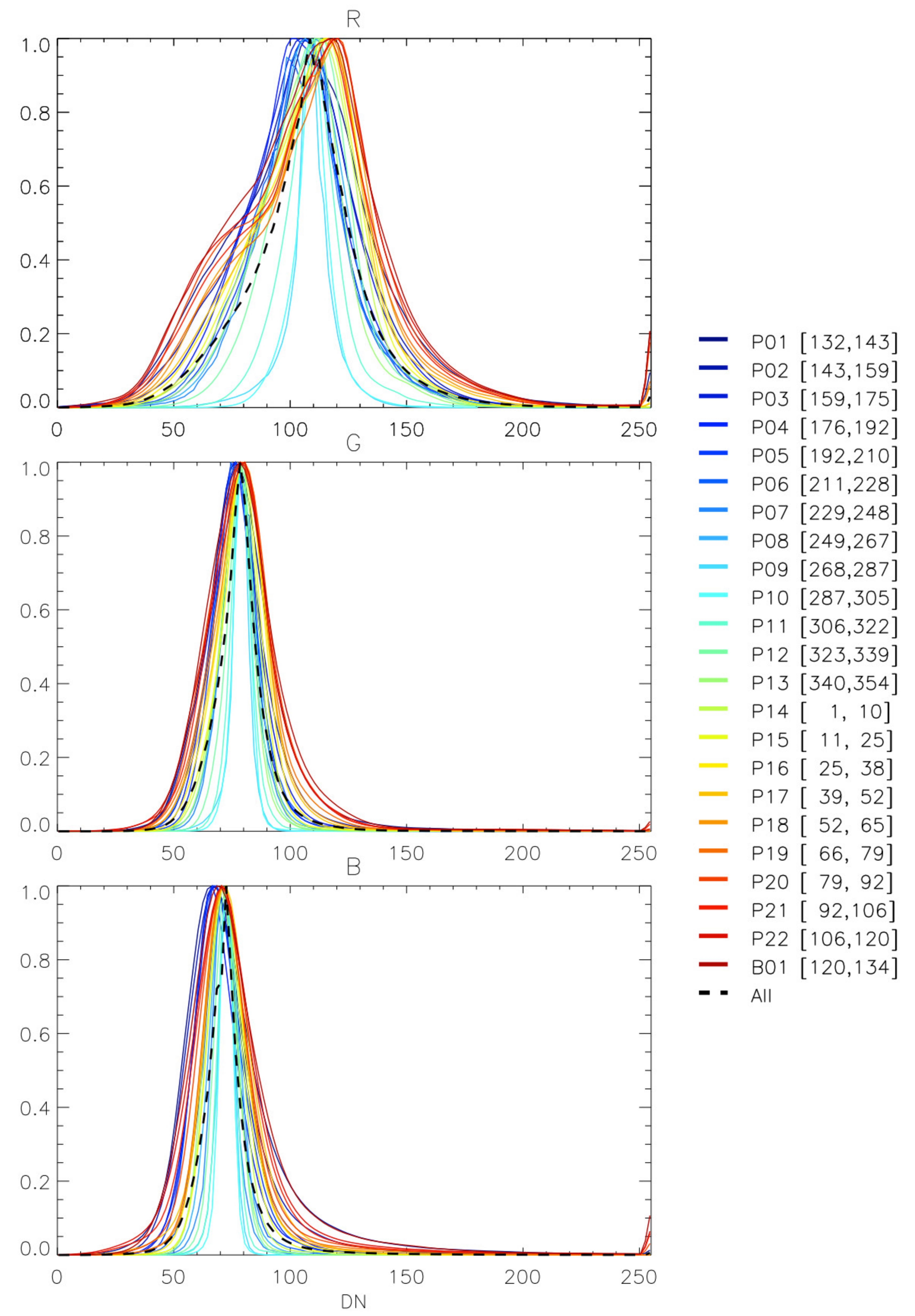
Despite the differences in photometric processing of different mission subphases, the RGB color composites have overall similar colors across the MRO mission. This is because a consistent color scheme is applied. For each channel, the median of each map is scaled to a fixed value and the resulting map is stretched so that a predefined range is linearly mapped to the Data Number (DN) range from 0 to 255. Figure 2 shows the resulting normalized DN distributions of the R, G and B channels for the area between 40° S and 40° N. For each channel, different subphases cluster around the overall distribution with only small shifts in the positions of the distribution modes. The G, B and most R curves have approximate Gaussian shape. Two-mode distribution is discernable in the R channel for the subphases in northern spring and summer (e.g., P18-B01), which reflects the higher surface albedo contrast in the longer wavelength for the less dusty period of the year. All three channels show the same tendency of narrower distributions for L_s = 249°–322° (P08–P11). This essentially reflects the reduced visible contrast due to the Mars year (MY) 28 global dust storm [32,35,37].

3. Method

This paper uses an image processing technique to distinguish clouds that are identifiable by eye in MDGMs. By definition, subvisible clouds are not included. The blue (B) and red (R) channels of the RGB color maps are used to derive daily cloud masks at the native standard MDGM resolution (0.1° × 0.1°). As will be explained in Section 3.1 and Section 3.2, the method follows three steps: (1) Select cloud candidates using the B channel; (2) filter out false positives by exploiting the B channel to R channel ratio; and (3) conduct quality control on the resulting cloud mask. The method is only semi-automatic as human decisions are involved at various stages to maintain the quality of computer-generated products. However, it is much more efficient than manually picking pixels of interest directly from each color MDGM. Before the details of the method are described in Section 3.1 and Section 3.2, the next few paragraphs define the cloud masks, justify the reasons for using the B and R channels, and provide some caveats.

In the cloud masks, non-cloudy pixels are set to zero, cloudy pixels are set to their adjusted DNs of the B channel MDGMs (Section 4.3), missing and excluded pixels are set to −999 to indicate invalid data.

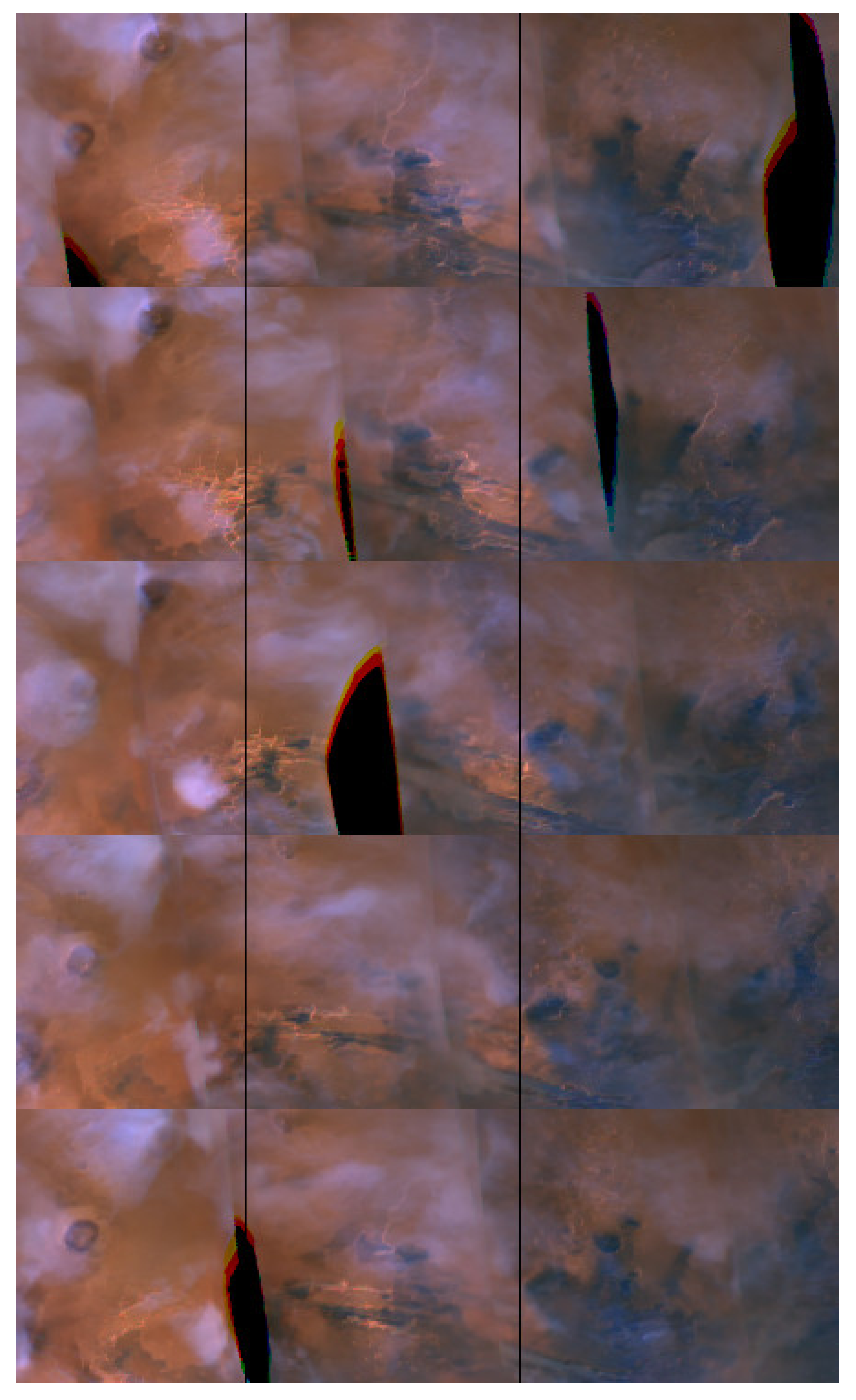
Among the R, G, and B channels of the color MDGMs, surface albedo features have the most contrast in the R channel and the least contrast in the B channel, clouds are the most apparent in the B channel and dust storms are the most apparent in the R channel (Figure 1). Thus, the B channel is most suitable for selecting candidate cloudy pixels. However, thick dust storms also appear quite bright in the B channel, though more so in the R channel (Figure 1 arrows). In other words, dust storms have smaller blue-to-red ratio than clouds, which is why clouds appear blueish and dust storms appear reddish in color MDGMs. The well-known color difference between Martian dust storms and condensate clouds was used to design the MARCI and other camera’s filters for the purpose of their distinction^{9, 31}. Interested readers can use the on-line interface of the Planetary Spectrum Generator (PSG) [38] (psg.gsfc.nasa.gov, accessed on 29 July 2021) to verify the effect of dust and clouds on the spectrum. In this paper, the ratios of the B to R channels are exploited to filter out the pixels affected by thick dust storms or surface features.

Although clouds may coexist with dust storms within a single pixel, the situation is not differentiable using MDGMs alone. Thus, the identified clouds should be considered as those that are not affected by apparent dust storms. As both surface ice deposits and atmospheric condensate clouds are bright in MDGMs, they cannot be differentiated based on pixel brightness alone. Although surface ice deposits can be filtered out based on their geographical locations and seasonal variations, further work is required to precisely determine where those pixels are in each MDGM. For simplicity, the pixels affected by polar caps are empirically excluded for each subphase in this study. For Hellas basin, it is sometimes possible to deduce that clouds exist above the seasonal ice deposit based on the morphology of the clouds in the vicinity of the region. Those pixels are preserved in the cloud mask. However, the corresponding DN values are contaminated by the high surface ice albedo, thus, they should not be used to compare with the cloud brightness in other areas.

3.1. Cloud Candidate Selection

To avoid subsequent complication in cloud detection, each color MDGM from P01 to B01 is visually inspected and the areas with apparent image processing defects are manually cropped out (e.g., Figure 1). After this preparation step, subsequent steps were performed one mission subphase at a time. This is one of the ways of handling possible complications associated with the image processing differences in MDGM construction (Section 2).

The cloud detection algorithm exploits the high brightness contrast between clouds and non-ice surface in blue images. Specifically, potential cloudy pixels in each MDGM are selected based on their DN deviations from a reference blue base map. The pixels with large positive deviations are deemed potentially cloudy and are assigned their original B channel DNs at this step (but will be adjusted in the final product—see Section 4.3), the pixels with negative or small positive deviations are deemed non-cloudy and are masked out with zero, the missing and excluded pixels are marked with −999. The workflow and details are described below.

(A) For each mission subphase, a blue base map composed of Data Numbers (DNs) without cloud influence is derived using the following procedure. (1) All the B channel maps within the subphase are stacked into a 3D array. At each horizontal pixel position, the smallest two DNs in the third dimension are discarded and the next smallest DN is chosen. The procedure is designed to minimize the influence of both clouds and potential low DN outliers in MDGMs. The resulting map is called “map0”. (2) Visual inspection is conducted on map0. If it is determined that some pixels are influenced by clouds, then those pixels are replaced with the non-cloudy DNs scaled from other subphases so that the mean DN in the neighborhood matches. The pixels to be replaced are chosen to be those above an empirical DN threshold through trials. A larger threshold leads to less pixels chosen, and vice versa. As an intermediate aid, map0 only needs to be reasonable and does not need to be accurate. It is intended to be used in combination with the detection criterion in step (B) to discriminate between large and small DN deviations. As the final cloud mask is required to pass a quality control step that manually corrects errors, a better combination of map0 and detection criterion will reduce the amount of manual work later on, therefore, it is desirable. When necessary, map0 is manually adjusted further in certain regions so that it works better with the selection criterion in (B). (3) The latitudes affected by polar caps are subjectively determined and excluded from map0. The result is the blue base map.

(B) The deviations of each B channel MDGM and the blue base map are calculated. A threshold for the deviations (called a “deviation threshold”) is chosen empirically for each subphase. This is carried out by iteratively examining the selected cloud candidates and adjusting the map0 versus deviation threshold pair. The pair is tuned until the visually obvious clouds in the batch of MDGMs are satisfactorily included and the inter-subphase consistency is maintained. The final choices for the deviation thresholds vary between 32 and 38 among the subphases and are specific to each subphase’s base map and MDGMs. The map0 and deviation threshold pair used in this paper is only one of the possible combinations that can serve the purpose of selecting cloud candidates.

3.2. False Positive Filtering and Quality Control

Thick dust storms may be mistaken for clouds in blue MDGMs (Figure 1) and need to be filtered out. In contrast to the B channel, the R channel shows large variations in surface albedo. Consequently, the B to R ratios vary strongly with geographical locations and are roughly anti-correlated with the albedos of the R channel. This makes it unsuitable to use a single B to R ratio threshold across the planet for filtering. Thus, a ratio’s ratio method is used instead. Specifically, the B to R ratio map for each day is divided by a reference B to R ratio map and the resulting map is evaluated against a specified ratio’s ratio threshold. As dust tends to make the B to R ratio smaller, the pixels with the ratio’s ratios below the threshold are probably affected by dust and are discarded. In theory, the ratio’s ratio threshold is 1.0; in practice, the ratio’s ratio threshold is set to 1.05. This is to account for the errors in image processing during the production of MDGMs and the errors associated with the construction of the reference B to R ratio map, as well as to avoid over-filtering cloudy pixels.

The reference B to R ratio map mentioned above is derived using the following procedure for each subphase. First, the median blue and the median red map for the subphase are derived, where each pixel in the median map adopts the median DN of all the days at that position. The ratio map of the median blue to the median red map is calculated. Clouds are searched in the median blue map using the procedure described in Section 3.1, and if found, the corresponding pixels in the ratio map are set to a missing value. The resulting ratio map is called “br2map0”. Next, the MDGM grid cells are classified into surface albedo bins with a bin size of 0.01 using a red Mars surface albedo map [39]. It is assumed that pixels with similar red surface albedos have similar B to R ratios, as the albedo is more uniform at shorter wavelengths. The median B to R ratio for each red surface albedo bin is calculated using the non-missing values in b2rmap0. Finally, each pixel of the reference B to R ratio map is assigned the value calculated for the corresponding red surface albedo bin.

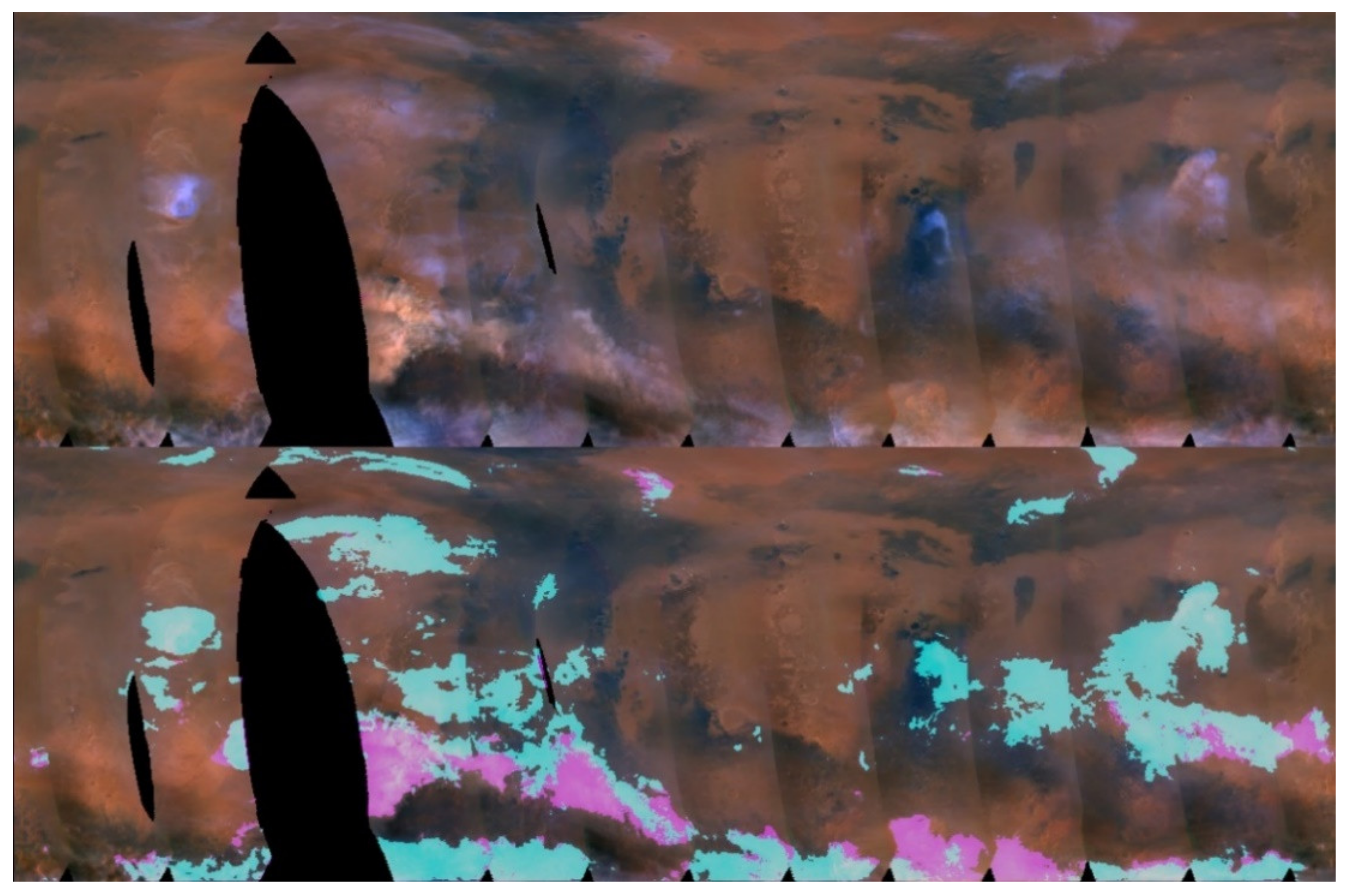
As an example, the bottom panel of Figure 3 shows the clouds identified before quality control for MY 28 L_s = 147°. The cloud candidates derived from the B channel (Section 3.1) are highlighted in two colors where the detected cloudy pixels (teal, to be retained) are separated from the others (pink, to be excluded) that are identified using the B to R ratio’s ratio method (Section 3.2). The technique generally works well for identifying obvious clouds and for filtering out false positives associated with surface albedo features or thick dust storms.

Quality control is conducted as the final step, where each cloud mask is visually inspected. Any residual false positives are deleted, and rare cases of false negatives are added manually. The quality control was conducted on a laptop computer with a screen size of 1536 × 864 pixels. Each cloud mask along with its corresponding MDGM (3600 × 1801 pixels) were downsized to fit on the screen for simultaneous visual inspection. Thus, not all errors can be eliminated due to this limitation, especially for those that are randomly scattered; in addition, human errors may exist but are difficult to quantify. Thus, extra care is needed for studies of local phenomena. In this paper, we use the cloud masks for large-scale studies where the fine details of the cloud masks are not essential for the conclusions. The overall DN histograms of the final cloudy and non-cloudy pixels classified in this paper can be found in Figure S1.

4. Results

The cloud masks are used to investigate the large-scale evolution and characteristics of the tropical cloud belt for 1 Mars year from MY 28 L_s = 132° to MY 29 L_s = 135° (from P01 to B01). The following applications take advantage of the cloud masks’ high spatial and temporal resolution as compared to other datasets.

4.1. Cloud Fraction Evolution

Figure 4 shows the daily cloud fraction between 35° S and 35° N as a function of L_s. Data from MY 28 L_s > 132° (to the right of the dashed line) and MY 29 L_s < 135° (to the left) are combined to show the annual evolution. The fraction is calculated as the ratio between the total area of cloudy pixels and the total area of non-missing pixels within the latitudinal band for each day. The MDGMs with >25% missing data are ignored. Data from different subphases (indicated by different colors) show generally good temporal continuity.

Figure 4 shows that clouds steadily build up coverage toward the peak (B01/P01) and rapidly decline afterwards. In MY 29, the cloud fraction gradually increases from ~0.01 at L_s = 20° to ~0.17 during L_s = 120°–130°. The timing of the peak is near the early-to-mid northern summer transition, in agreement with the MARCI UV result [14] which also shows that the peak of the tropical cloud belt is skewed later than that for the TES IR result [11].

In MY 28, the rapid cloud belt dissipation exhibits notable oscillatory behavior. The cloud fraction sharply drops from ~0.22 to ~0.15 within a week of L_s = 132°. It shows an apparent secondary peak of ~0.21 near L_s = 144° (Section 4.4) and quickly collapses to <0.1 by L_s = 149°. Active dust storms occurred in the southern mid-latitudes during L_s = 137°–160°. In particular, several intense dust storm episodes are observed extending from the south seasonal cap edge northward into the tropical cloud belt in the Argyre-Solis-Valles Marineris (ASV), Hellas-Tyrrhena, and Cimmeria-Sirenum regions [34]. These dust storms may have contributed to the disintegration of the cloud belt. The cloud fraction remains <0.01 during L_s = 220°–360° in MY 28 (Figure 4). Clouds are not observed during the time period affected by the MY 28 global dust storm (L_s = 265°–320°)—even the clouds over Arsia Mons have disappeared, while they usually persist throughout the year in other Mars years [21].

4.2. Cloud Frequency Evolution

Figure 5 shows the evolution of the tropical cloud belt in terms of the cloud occurrence frequency for each mission subphase (corresponding to a month). For each pixel, the cloud occurrence frequency is calculated by dividing the number of days clouds are present by the number of days data are available. The latitudes affected by polar caps in each subphase are excluded (Section 3). As found by numerous previous studies, e.g., [10,11,14,15,27], clouds in the low latitudes are widespread in the aphelion season and are almost absent in the perihelion season. The decay in late northern summer, development in northern spring and peak in early-mid northern summer are clearly seen. In addition to the major volcanoes (Olympus, Alba, Ascraeus, Pavonis, Arsia, and Elysium Mons), other hot spots of frequent cloud cover include Valles Marineris, Syrtis Major and Hellas Planitia. These are most obvious during L_s = 39°–159° (P17–B01 and P02). For Hellas, strictly speaking, MDGMs suggest the existence of clouds near the edge of the basin based on cloud morphology, the existence of clouds within Hellas cannot be determined in the absence of other information.

Figure 5 examines the cloud belt from the perspective of how often clouds occur at each location within a month. In this representation, the cloud belt appears zonally noncontiguous, with less frequent or absent clouds in the Arabia Terra and Amazonis Planitia longitudinal sectors. The cloud belt is most obvious in B01 (L_s = 121°–135°) when hot spots are connected by areas with less frequent clouds in other longitudes. However, the occurrence of clouds within the belt appears meandrous, with large variations in the centroid latitudes. The widest latitudinal extent occurs near Valles Marineris and the thinnest near Amazonis Planitia. Thus, description of the tropical cloud belt needs to consider its zonal variation.

In the southern hemisphere, there is a notable cloud branch diverting from the main cloud belt. The cloud branch extends from the Valles Marineris towards the Noachis/Hellas region in an approximate northwest–southeast direction during L_s = 93°–143° (P21–B01 and P01, Figure 5). The feature was previously noted in MGS MDGMs [20]. A hint can be glimpsed from the MGS TES and MRO MARCI UV results, though the spatial and temporal binning of those datasets likely smeared most of it out [14]. Another cloud branch from Tyrrhena Terra toward Hesperia Planum (to the northeast of Hellas) is suggested in P22, B01 and P01, though it is less obvious because of the shorter length.

In the northern hemisphere, clouds are sometimes observed to the north and northeast of Tharsis in northern mid-summer (B01 and P01, Figure 5). These are annular clouds recurring each year near the edge of the north polar cap [22]. Clouds are also observed to the northeast of Arabia Terra in this season. These are often irregular and occasionally arc shaped. These mid-summer clouds are not part of the polar hood which begins to form after L_s ~160° [20]. The polar hoods cannot be systematically studied here because of the exclusion of the high latitudes, though the edges of the polar hoods can be seen in some subphases, including the zonal wavenumber 2 pattern [8] of the north polar hood in P06, P07 and P11.

4.3. Brightness Evolution

As determined by the nature of the MDGMs, quantitative cloud optical depths are not provided in this study. Nonetheless, the Data Numbers (DNs) of the cloud masks can qualitatively differentiate how reflective the clouds are, and thus can serve as a proxy for cloud optical thickness under the assumption that brighter clouds tend to be thicker (Figure S2). To account for the small differences in the DN distributions among different subphases (Figure 2 bottom panel, color lines), the original blue DNs of each subphase are shifted so that the mode of the distribution aligns with that of the overall distribution (Figure 2 bottom panel, black dashed line). If there are values above 255 as a result of the shift, those values are set to 255. The adjusted DNs are assigned to the cloudy pixels in the final cloud masks and are used in the brightness-related analyses in this paper.

The left column of Figure 6 shows the mean cloud masks for the subphases with widespread clouds. The value at each pixel is the average of non-negative cloud mask values with respect to the number of days MDGMs that are available within the subphase. Thus, non-cloudy pixels (with zero values) reduce the mean and the result mimics a simple mean cloud brightness within a month of time. An exception is Hellas in winter, when surface ice cannot be separated from clouds based on visible images alone, as a result, those DNs are not representative of clouds. The major volcanoes show the brightest clouds, followed by the general Valles Marineris and Syrtis Major regions. These areas also tend to have the most frequent cloud cover (Figure 5) and the thickest cloud optical depths [11,14].

However, the low latitude clouds in the mean cloud masks appear to be less spatially extensive than those in the MARCI UV optical depths [14]. For example, the mean cloud masks indicate a break in Amazonis (near 170° W) even when the cloud belt is the most extensive (Figure 6 B01 L_s = 121°–135°); in comparison, the MARCI UV optical depths for L_s = 90°–120° show a zonally contiguous tropical cloud belt, though those for L_s = 120°–150° suggest a break there [14]. This probably reflects that the UV filter is more sensitive to clouds than the blue filter, thus, the UV observations can detect thinner clouds which are not obvious in the color MDGMs. Furthermore, the MARCI UV results were averaged over MY 28–34 within each 30° L_s bin [14], while the cloud mask here is for MY 28–29 only; thus, there may also be differences due to interannual variability. The MGS TES optical depths [11] also show a contiguous tropical cloud belt for the relevant L_s periods, though the TES observations are for different local time (1400 LT) and Mars years (MY 24–26), and there is appreciable variability even within one hour of local time [14] (Section 4.5).

The right column of Figure 6 shows the mean cloud DN, i.e., the average DNs of the cloudy pixels with respect to the number of cloudy days within the subphase. As non-cloudy pixels do not contribute here, the values are larger than those in the left column. In most cases, hot spots match in both columns, e.g., the volcanoes, Valles Marineris, and Syrtis Major. However, there are some differences, as the right column depicts the mean brightness of clouds when they occur. For example, the mean cloud DNs to the northeast of Tharsis and to the northeast of Arabia during L_s = 121°–143° (B01, P01) can be almost as bright as those over the volcanoes in the right column, but the corresponding mean cloud masks in the left column are much muted because the clouds occur less frequently and move from day to day during the time period. In P21 (L_s = 93°–106°), Syrtis Major is a local hot spot in the mean cloud mask on the left, but not so much in the mean cloud DN on the right, which suggests frequent occurrence of relatively thin clouds. In the subsequent time period P22 (L_s = 106°–120°), Syrtis Major is a hot spot in both the mean cloud DN (right) and the mean cloud mask (left), indicating a thickening of clouds in the area. This tendency can also be seen in Figure S4, which will be discussed further in the next section.

4.4. Zonal Oscillation of Tropical Clouds

For most of the existing cloud datasets, spatial and temporal binning on a coarse grid is needed to describe the general cloud distribution. As a result, important details at finer scales can be missed. The cloud masks derived from the MDGMs have 0.1° × 0.1° spatial resolution and daily coverage, providing an opportunity to systematically examine cloud distribution on these scales. Figure 7 shows the time evolution of the equatorial clouds (within 20° S–20° N in 5° latitudinal intervals) during L_s = 132°–159° of MY 28 (P01 and P02) using Hovmöller diagrams which depicts the longitude versus time variation. The top panel shows the DNs of the clouds in the cloud masks as a function of longitude and time; the bottom panel shows the deviations of the DNs from the time mean at each longitude.

Apparent brightening is seen in the 60° E–180° E sector during L_s ≈ 139°–147° (Figure 7). The brightening starts from Syrtis Major and extends eastward with time. It corresponds to the second peak in the cloud fraction curve during the decay of the tropical cloud belt in Figure 4. During this time period, clouds in the opposite hemisphere are suppressed. Before and after this time period, clouds are present in the Tharsis and Valles Marineris longitudinal sector (130° W–0°), but clouds are poorly developed or absent in the 60° E–180° E sector. The oscillation of clouds between the two longitudinal sectors suggests an eastward propagating wave with a wave period of about 20–30 sols, though the lack of clouds in the 0°–60° E and 180° W–130° W sectors makes disruptions.

Cloud formation depends on atmospheric temperature, water vapor abundance, and condensation nuclei. As the decline of the tropical cloud belt is known to be sensitive to atmospheric temperature [40], it is useful to examine atmospheric waves in model simulated temperatures in the tropics. Figure 8 shows the eddies in the temperature field at 2.5° S and the p = 130 Pa pressure level (z = 15 km pseudo height calculated as $z=10·ln\left(610/p\right)$ where pressure p is in Pa) derived from the OpenMARS data assimilation product (5° longitude × 5° latitude) [41] for MY 28 L_s = 131°–160°. Wavelet analysis [42] is performed to decompose the transient eddies into components with wave periods P < 2 sol, P = 2–9 sol and P > 9 sol. Fourier analysis is then performed on the P > 9 sol eddies to extract eastward and westward propagating waves with various zonal wave numbers and wave periods.

Figure 8a shows that temperature is increasing during L_s = 131°–160° which is consistent with the overall decline of the tropical cloud belt. After the removal of the trend for each longitude and along with it, the stationary wave component, Figure 8b shows that the temperatures are lower during L_s ≈ 139°–148° which corresponds to the time period for cloud brightening in and east of Syrtis Major. Additionally, various propagating waves are superimposed on the eddy temperature field (Figure 8b). As shown in Figure 8c, large-scale waves with zonal wavenumbers k = 0–3 and wave periods P > 9 sol are important components of the eddies. They appear to be dominated by zonally symmetric variation and eastward propagating waves, with a hint of westward propagating waves.

The eastward propagating k = 1 waves (Figure 8d) are dominated by a P = 20–30 sol wave during L_s ≈ 140°–152°. The wave is latitudinally symmetric about the equator within 10°–15° N/S (Figure 8e). There is minimal vertical phase tilt below z ≈ 20–25 km (Figure 8f). The meridional wind component (v’) of the wave vanishes at the equator (not shown). The latitudinal width of the wave is about 2–3 equatorial radius of deformation ($a_e=\sqrt{c/\left(2\beta \right)}$, where c is the phase speed of the wave, β = 2Ω/R at the equator, Ω is the planet rotation rate and R is the planet radius). The wave structure seems to conform to that of an equatorial Kelvin wave [43]. Significant wave amplitudes also exist at higher latitudes (Figure 8e), but those waves have different structures and can exist even when the equatorial wave is absent. Wave analysis for an independent data analysis product EMARS [44] also shows a prominent eastward propagating P = 20–30 sol wave with zonal wavenumber k = 1 along the equator during this time period, despite the differences in the details of other wave components (Figure S3).

The brightening of clouds in the Syrtis/Elysium sector and the darkening of the clouds in the Valles Marineris sector coincide with the cold and warm phases of the wave’s temperature field below z ~20 km altitude. Thus, the equatorial Kelvin wave may help explain the zonal oscillation of the tropical cloud belt if the observed clouds are mainly below z ~20 km. The daytime low latitude MRO Mars Climate Sounder (MCS) limb profiles of cloud optical depth seldomly reach below 20 km altitude in northern spring and summer due to opaque clouds along the line-of-sight within the lowest couple of scale heights [13,27], though this evidence is indirect. The phase reversal of the Kelvin wave near z ~20–25 km (Figure 8f) could be related to the radiative effect of clouds, as strong nighttime radiative cooling at the cloud level can induce substantial adiabatic heating from above, which tends to shift wave phases [45].

Cloud brightening in and east of Syrtis Major during the disintegration of the tropical cloud belt was noted in MGS MDGMs for MY 24 [20]. Although cloud mask is only derived for one Mars year in this paper, an inspection of the MGS and MRO MDGMs for MY 24–32 shows that the phenomenon occurred almost every year near L_s = 140° and lasted for about 4°–9° of L_s each time (

Table 1. L_s period for cloud brightening in and east of Syrtis Major after L_s = 135° for each Mars year between MY 24 and 32. The - sign denotes none observed.

MY	24	25	26	27	28	29	30	31	32
Ls range	142°–146°	137°–146°	142°–147°	-	139°–147°	-	141°–147°	145°–149°	145°–150°

). The only exceptions are MY 27 and MY 29 when no brightening in the eastern hemisphere was observed after L_s ~140°. In MY 29, an intense dust storm episode occurred in the ASV and surrounding regions during L_s = 137°–148°, which significantly changed atmospheric thermal structure and waves [34,45] In MY 27, a significant dust storm episode occurred in the area between Valles Marineris and Hellas during L_s = 133°–137° which appeared to result in an early termination of the tropical cloud belt that year [24,34]. As suggested in Figure S4, there appears to be simultaneous cloud brightening in the eastern hemisphere and cloud suppression in the western hemisphere during L_s = 110°–120° in MY 29. Thus, there could be other episodes of large-scale long-period tropical cloud oscillations before L_s ~140°, though the data available for MY 28 only covered one.

4.5. Local Time Variation

Strong diurnal variations of Martian clouds have been demonstrated in the literature, e.g., [15,26,46]. Although MRO is in a 0300–1500 LT sun-synchronous orbit, the wide-angle MARCI image swath covers about an hour off-nadir in each direction toward the limb [14,30]. Significant local time variation in MARCI UV cloud optical depths has been shown [14], despite the limited local time coverage. In MDGMs composed from the MARCI visible images, the signal is hidden behind an artificial “wave” that stems from the convolution of the diurnal cycle of the clouds and the periodicity of the MRO orbit. The argument was used before to explain the periodicity in the cloud areas observed in the MGS MOC wide-angle images [21].

In addition to the low frequency cloud oscillation discussed in Section 4.4, Figure 7 shows extremely regular higher frequency variations in the form of an eastward propagating wave with a wave period of approximately 5 days. Another example of the suspiciously regular wave can be seen in Figure S4. This periodicity corresponds to MRO’s ground track shift pattern [29]. Specifically, the MRO orbits have a ~5-day repeat cycle (embedded within a ~17-day repeat cycle) such that a 5-day sweep divides the interval between adjacent orbit tracks into roughly equal segments. As the local time increases from the left limb to the right limb in a MARCI swath, if appreciable local time variation exists for an observable, it will aggregate over time into an artificial ”traveling wave” that is tied to the spacecraft’s orbit.

To illustrate the effect, Figure 9 shows the area within 15° S–15° N and 120° W–0° for 5 consecutive days from the top to the bottom. The 5-day MRO orbit pattern is indicated by the shift of the MARCI swath edges from the left to the right between the vertical lines. Along each vertical line, clouds are generally more extensive in the top panel where they are located closer to the right limb of the corresponding image swath (later in local time); clouds appear progressively less extensive in subsequent days when they approach the left limb (earlier in local time). This implies generally more clouds for 1500–1600 LT than for 1400–1500 LT which is consistent with other studies’ findings of increasing clouds during the afternoon hours [14,15,26].

5. Summary and Discussion

Cloud masks have been derived from the Version 2 MRO MARCI Mars Daily Global Maps (MDGMs) for 1 Mars year (from MY 28 L_s = 132° to MY 29 L_s = 135°) using a semi-automatic image processing technique. Changes between the Version 1 and Version 2 MDGMs are descried. The blue channel map of each color MDGM is used to select cloud candidates, and the blue-to-red ratio’s ratio is used to filter out false positives. Manual quality control is conducted through visual inspection. The cloud masks are on MDGM’s native 0.1° longitude × 0.1° latitude grid and are available each day. In the cloud masks, non-cloudy pixels are set to zero, cloudy pixels are set to their adjusted Data Numbers of the blue channel maps (Section 4.3), missing and excluded pixels are set to a special number (−999).

In this paper, the derived cloud masks are used to investigate the large-scale evolution and characteristics of the tropical cloud belt on Mars, with a focus on a few aspects that benefit from the high spatial and temporal resolutions. The main results are summarized below.

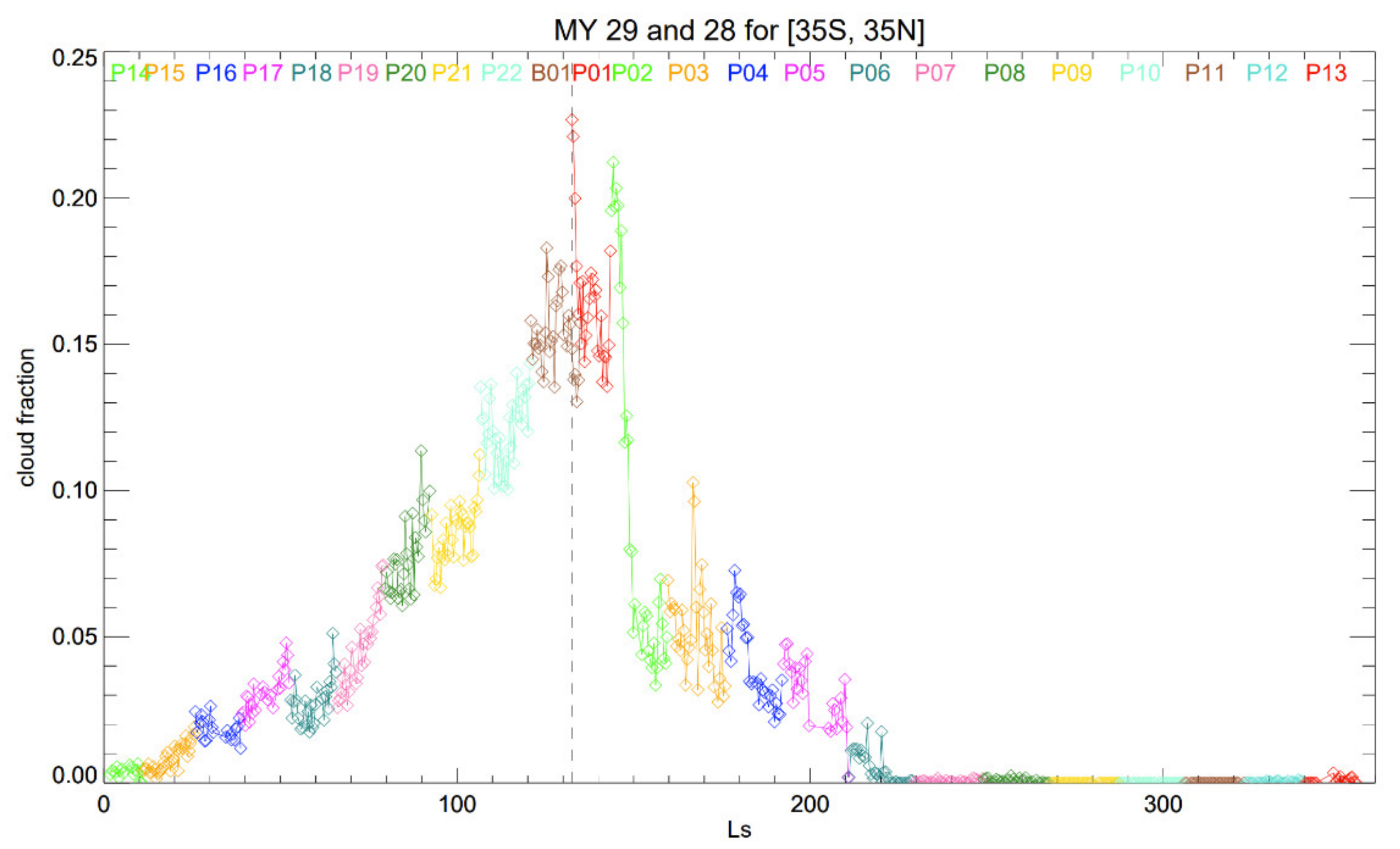
The fraction of cloudy area between 35° S and 35° N gradually increased from ~1% at L_s = 20° to ~17% near L_s = 125° in MY 29. The timing of the peak was near the early-to-mid northern summer transition, which agrees with the MARCI UV result [14] but not with the TES IR results [11]. In MY 28, the cloud fraction sharply dropped from ~22% to ~15% within a week of L_s = 132°, a secondary peak of 21% occurred near L_s = 144° and was associated with a large-scale zonal cloud oscillation, the cloud belt quickly collapsed afterwards, to which several dust storms may have contributed. Clouds were not identified in MDGMs during the time period affected by the MY 28 global dust storm.

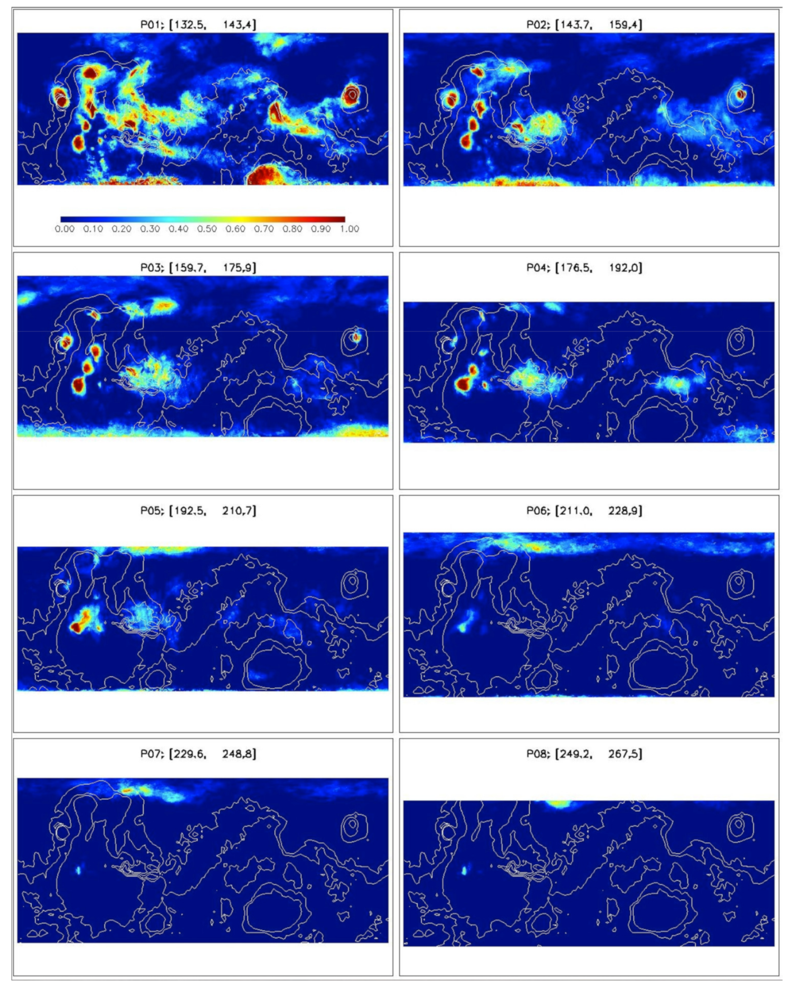
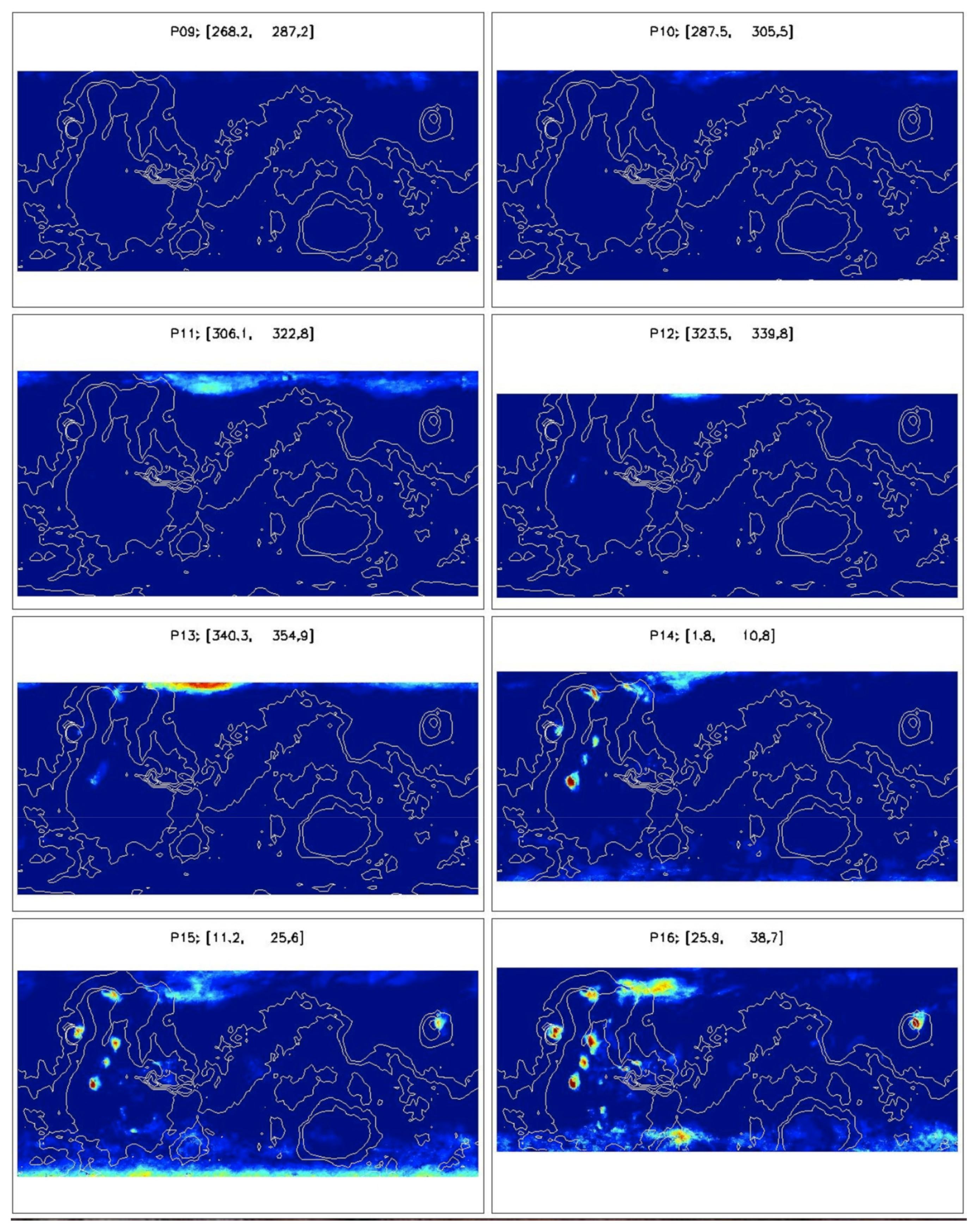
Monthly cloud occurrence frequency represents how often clouds occur at each location. It demonstrates the cloud belt’s development in northern spring, peak in early/mid northern summer, and decay in late northern summer. From this perspective, the cloud belt appears zonally noncontiguous and meandrous. A notable cloud branch diverts from the main cloud belt and extends from Valles Marineris toward Noachis during L_s = 93°–143°. These observations highlight the need to better characterize the zonal variability of the tropical cloud belt.

It should be noted that the MARCI images used in the MDGMs are taken from the 0300–1500 LT sun-synchronous MRO orbit. The Martian atmosphere has a rich mix of vigorous thermal tides which will be aliased into observations made at nearly fixed local time [47,48]. As clouds and thermal tides are intricately linked with each other [4,45], it is inevitable that the effects of thermal tides are embedded within MDGMs’ cloud observations. 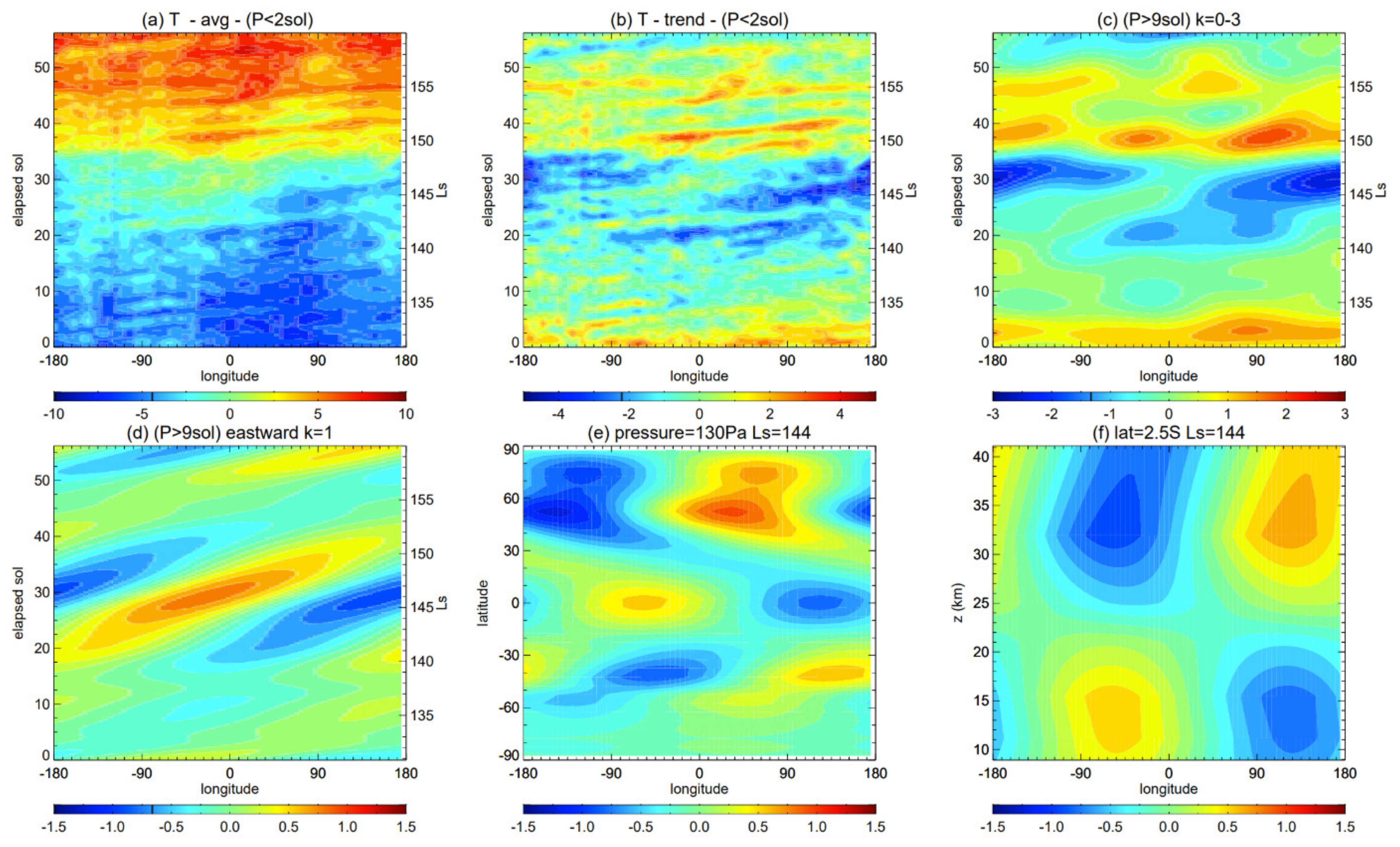Apparent zonal variations are observed in temperatures sampled at fixed local time [47,48,49]. Warmer temperatures would favor gaps or underdeveloped sectors in the tropical cloud belt if the clouds are sensitive enough to the perturbations. However, the pattern of the eddy temperatures changes significantly with altitude due to tidal modes of different wavelengths and phases (Figure S5), thus, the relationship between clouds and thermal tides can be quite complicated, and requires further study.

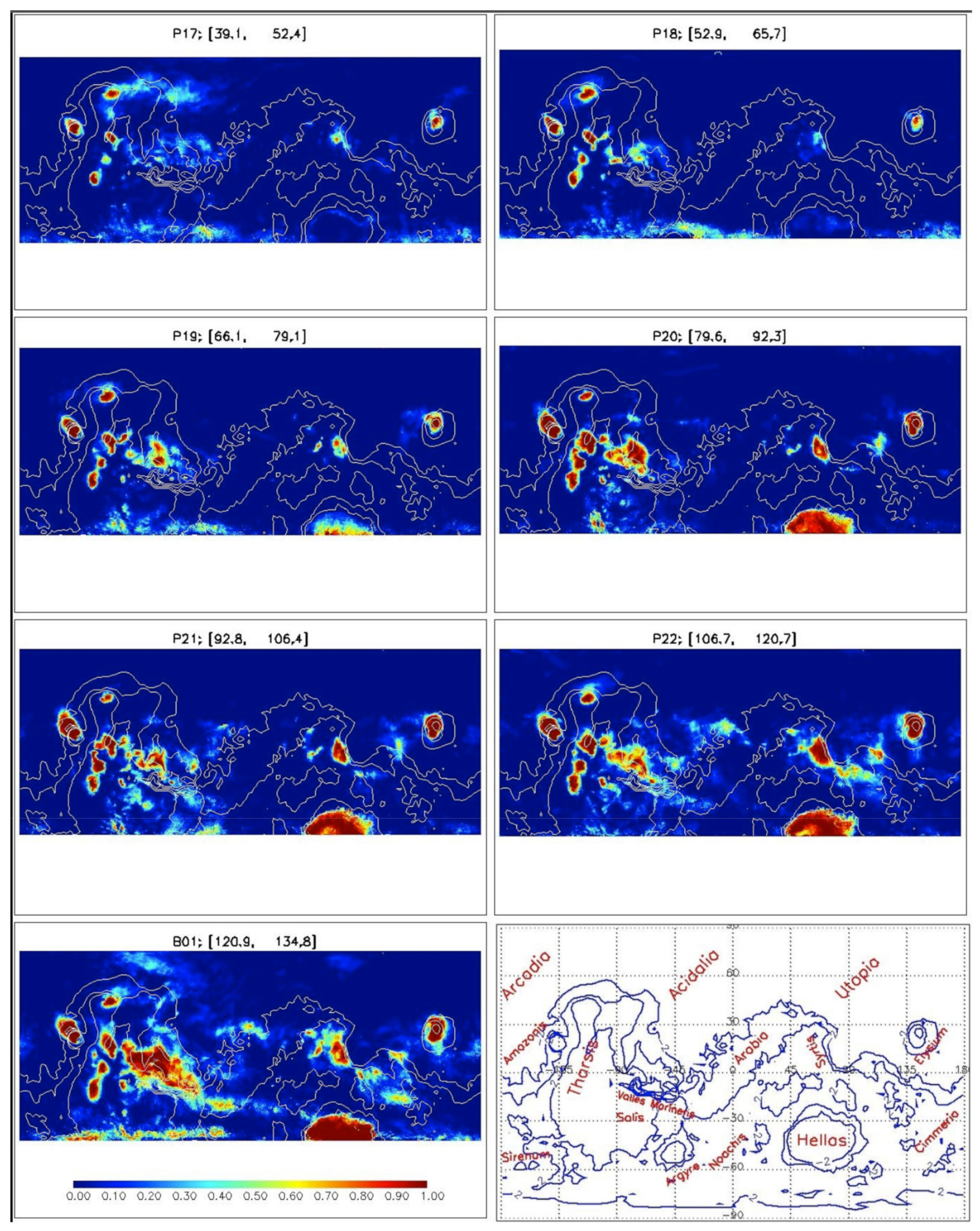
The cloud masks can qualitatively differentiate how reflective clouds are, and thus serve as a proxy for cloud optical thickness. The major volcanoes show the brightest clouds, followed by the general Valles Marineris and Syrtis Major regions. These regions also tend to have the most frequent cloud cover. However, there are also regions where thick clouds occur infrequently or thin clouds occur frequently. The information may become lost in a simple time mean. The low latitude clouds in the mean cloud masks appear to be less spatially extensive than those in the MARCI UV optical depths [14]. Among other possibilities, this probably reflects the higher sensitivity of the UV images than the blue images to clouds.

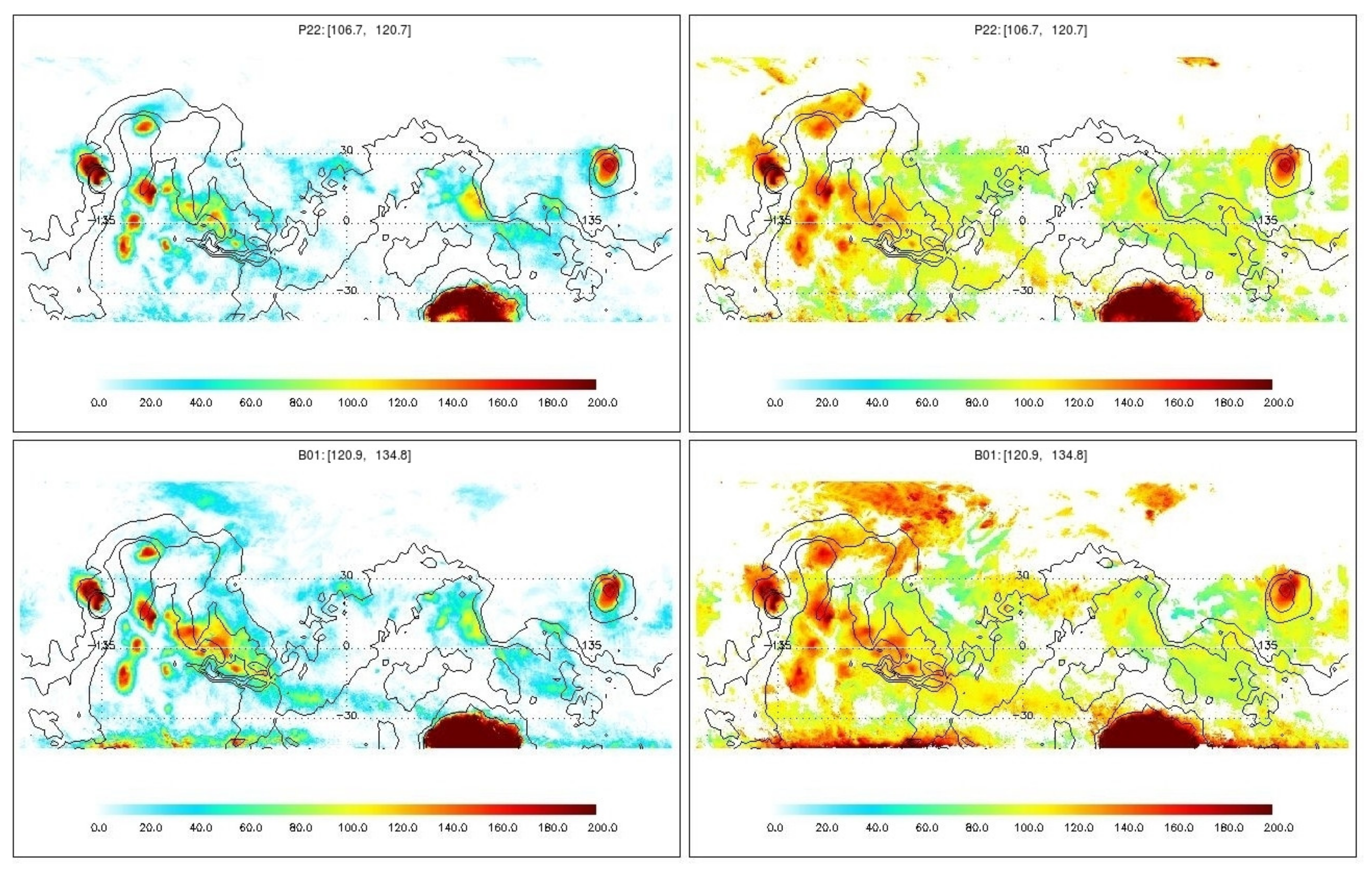
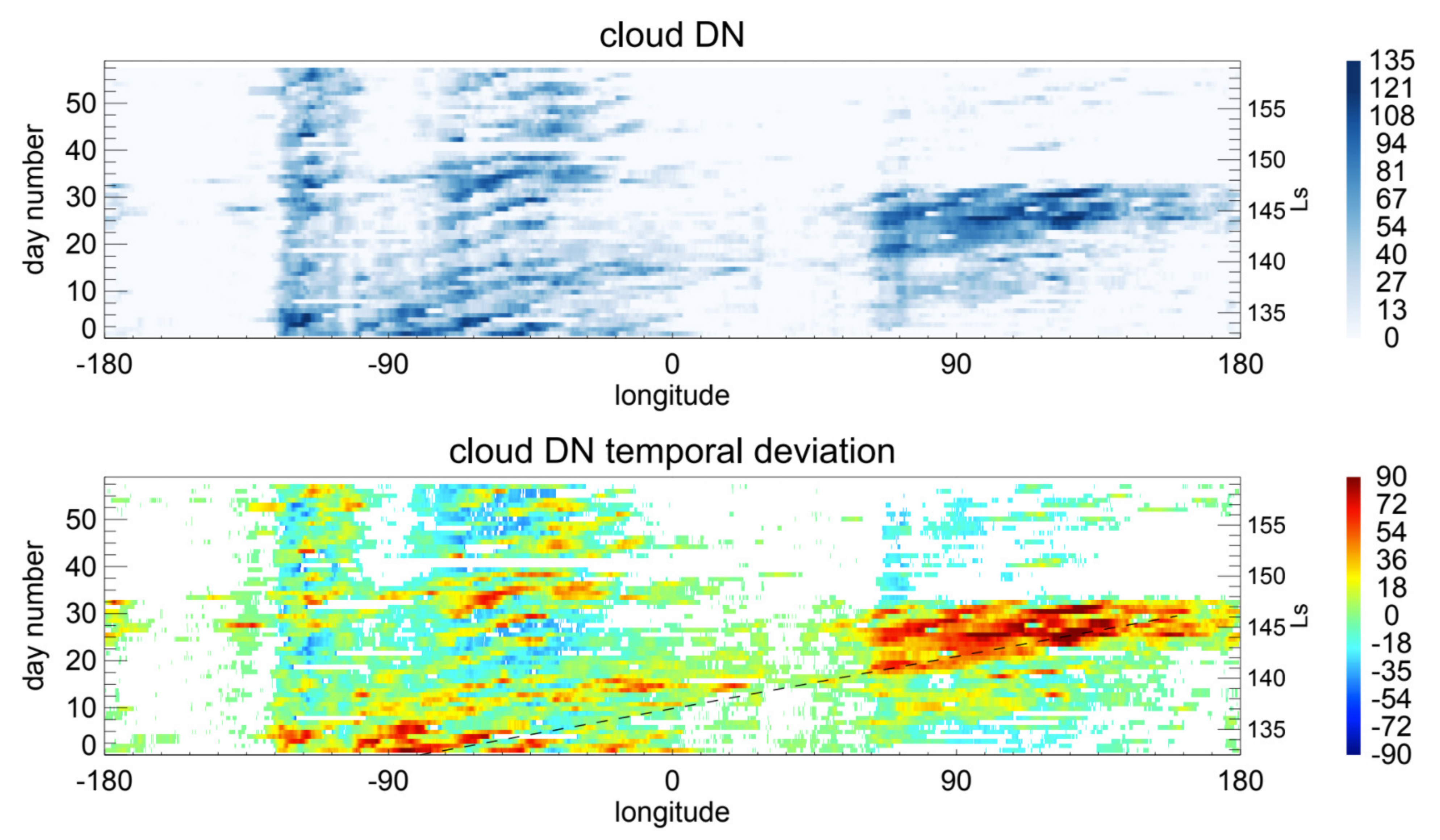
An interesting finding is the zonal oscillation of the clouds within the tropical cloud belt. During the decay of the tropical cloud belt in MY 28, apparent cloud brightening is observed in the eastern hemisphere (in and east of Syrtis Major) while clouds in the western hemisphere (around Valles Marineris) are suppressed. Cloud brightening in Syrtis Major was mentioned before for the MGS era [20], and several papers reported a related phenomenon called “blue clearing” where the disappearance of clouds in Syrtis Major reveals the surface albedo feature in telescopic images [50,51]. However, cloud brightening and blue clearing were not previously recognized as part of an oscillation within the tropical cloud belt. In this paper, the tropical cloud oscillation is found to occur each Mars year around L_s ~140° and last for a few degrees of L_s between MY 24 and MY 32, except for MY 27 and 29 when intense dust storms disrupted the pattern. The oscillation may be easier to spot in images during the disintegration of the tropical cloud belt because the distribution of clouds during this time period is quite sensitive to the temperature perturbations associated with eddies [52]. However, additional large-scale long-period tropical cloud oscillations may exist before L_s ~140° each year (Figure S4).

The oscillation of the tropical cloud belt appears to be associated with an eastward propagating zonal wavenumber k = 1 with a wave period P between 20 and 30 sols. The wave is symmetric about the equator and is confined within 10°–15° N/S. The wave structure conforms to that of an equatorial Kelvin wave. Previous studies of Kelvin waves in the Martian atmosphere are mostly about the diurnal or semidiurnal non-migrating thermal tides, e.g., [49,53,54,55,56]. A P = 2.5 sol Kelvin wave was also identified in the middle and upper atmosphere [57]. The Kelvin wave discussed here has a much narrower latitudinal width and a much longer wave period. It coexists with other circulation components to affect atmospheric conditions and can be an important factor for the intra-seasonal variability of the Martian tropical cloud belt.

The wide-angle MARCI images provide only limited local time coverage; however, change in clouds with local time is still observable. The signal is hidden in the cloud mask as a highly regular 5-day traveling wave that stems from the convolution of the diurnal cycle of Martian clouds and the orbital cycle of the MRO spacecraft. The argument was previously used to explain an artificial signal in the clouds observed in MGS MOC wide angle images [21]. It should be noted that eddies with periodicity around 5 sols are present in the data assimilation products (Figure 8 and Figure S3), thus, physical presence of the wave cannot be ruled out. However, it is not clear if or by how much the assimilations are affected by the forcing periodicity of the input MRO data. Additional data from different satellite orbits may help clarify.

Cloud masks do not contain quantitative optical depths due to the nature of MDGMs. Nevertheless, cloud masks derived here can be useful for a number of applications, such as analyzing cloud distributions, comparing with simulation results and other observations, filtering in or filter out clouds for various applications, Supplementing Information from other datasets, training and testing machine learning algorithms, etc. It is hoped that the product can be helpful for the community to better understand the Martian atmosphere. The cloud masks can be found on Harvard Dataverse at https://doi.org/10.7910/DVN/WU6VZ8 (accessed on 29 July 2021).

References

1. Clancy, R.T.; Montmessin, F.; Benson, J.; Daerden, F.; Colaprete, A.; Wolff, M.J.; Haberle, R.M.; Forget, F.; Smith, M.D.; Zurek, R.W. Mars Clouds. In Atmospere and Climate of Mars; Haberle, R.M., Clancy, C.T., Forget, F., Smith, M.D., Zurek, R.W., Eds.; Cambridge University Press: Cambridge, UK, 2017. [Google Scholar]
2. Hinson, D.P.; Wilson, R.J. Temperature inversions, thermal tides, and water ice clouds in the Martian tropics. J. Geophys. Res. Planets 2004, 109, E01002. [Google Scholar] [CrossRef]
3. Kleinböehl, A.; Wilson, R.J.; Kass, D.; Schofield, J.T.; McCleese, D.J. The semidiurnal tide in the middle atmosphere of Mars. Geophys. Res. Lett. 2013, 40, 1952–1959. [Google Scholar] [CrossRef]
4. Wilson, R.J.; Guzewich, S.D. Influence of water ice clouds on nighttime tropical temperature structure as seen by the Mars Climate Sounder. Geophys. Res. Lett. 2014, 41, 3375–3381. [Google Scholar] [CrossRef]
5. Navarro, T.; Madeleine, J.B.; Forget, F.; Spiga, A.; Millour, E.; Montmessin, F.; Maattanen, A. Global climate modeling of the Martian water cycle with improved microphysics and radiatively active water ice clouds. J. Geophys. Res. Planets 2014, 119, 1479–1495. [Google Scholar] [CrossRef] [Green Version]
6. Kahre, M.A.; Hollingsworth, J.L.; Haberle, R.M.; Wilson, R.J. Coupling the Mars dust and water cycles: The importance of radiative-dynamic feedbacks during northern hemisphere summer. Icarus 2015, 260, 477–480. [Google Scholar] [CrossRef]
7. Lee, C.; Richardson, M.I.; Newman, C.E.; Mischna, M.A. The sensitivity of solsticial pauses to atmospheric ice and dust in the MarsWRF General Circulation Model. Icarus 2018, 311, 23–34. [Google Scholar] [CrossRef]
8. Haberle, R.M.; Kahre, M.A.; Barnes, J.R.; Hollingsworth, J.L.; Wolff, M.J. MARCI observations of a wavenumber-2 large-scale feature in the north polar hood of Mars: Interpretation with the NASA/Ames Legacy Global Climate Model. Icarus 2020, 335, 113367. [Google Scholar] [CrossRef]
9. James, P.B.; Christensen, P.R.; Clancy, R.T.; Lemmon, M.T.; Withers, P.; Haberle, R.M.; Forget, F.; Smith, M.D.; Zurek, R.W. History of Mars Atmosphere Observations. In Atmospere and Climate of Mars; Haberle, R.M., Clancy, C.T., Forget, F., Smith, M.D., Zurek, R.W., Eds.; Cambridge University Press: Cambridge, UK, 2017. [Google Scholar]
10. Tamppari, L.K.; Zurek, R.W.; Paige, D.A. Viking era water-ice clouds. J. Geophys. Res. Planets 2000, 105, 4087–4107. [Google Scholar] [CrossRef] [Green Version]
11. Smith, M.D. Interannual variability in TES atmospheric observations of Mars during 1999–2003. Icarus 2004, 167, 148–165. [Google Scholar] [CrossRef]
12. Smith, M.D. THEMIS observations of Mars aerosol optical depth from 2002–2008. Icarus 2009, 202, 444–452. [Google Scholar] [CrossRef] [Green Version]
13. Kleinböehl, A.; Schofield, J.T.; Kass, D.M.; Abdou, W.A.; Backus, C.R.; Sen, B.; Shirley, J.H.; Lawson, W.G.; Richardson, M.I.; Taylor, F.W.; et al. Mars Climate Sounder limb profile retrieval of atmospheric temperature, pressure, and dust and water ice opacity. J. Geophys. Res. Planets 2009, 114, E10006. [Google Scholar] [CrossRef]
14. Wolff, M.J.; Clancy, R.T.; Kahre, M.A.; Haberle, R.M.; Forget, F.; Cantor, B.A.; Malin, M.C. Mapping water ice clouds on Mars with MRO/MARCI. Icarus 2019, 332, 24–49. [Google Scholar] [CrossRef]
15. Giuranna, M.; Wolkenberg, P.; Grassi, D.; Aronica, A.; Aoki, S.; Scaccabarozzi, D.; Saggin, B.; Formisano, V. The current weather and climate of Mars: 12 years of atmospheric monitoring by the Planetary Fourier Spectrometer on Mars Express. Icarus 2021, 353. [Google Scholar] [CrossRef]
16. Olsen, K.S.; Forget, F.; Madeleine, J.B.; Szantai, A.; Audouard, J.; Geminale, A.; Altieri, F.; Bellucci, G.; Oliva, F.; Montabone, L.; et al. Retrieval of the water ice column and physical properties of water-ice clouds in the martian atmosphere using the OMEGA imaging spectrometer. Icarus 2021, 353, 113229. [Google Scholar] [CrossRef]
17. Gierasch, P.; Thomas, P.; French, R.; Veverka, J. Spiral clouds on Mars: A new atmospheric phenomenon. Geophys. Res. Lett. 1979, 6, 405–408. [Google Scholar] [CrossRef]
18. Kahn, R. The Spatial and Seasonal Distribution of Martian Clouds and some Meteorological Implications. J. Geophys. Res. Space Phys. 1984, 89, 6671–6688. [Google Scholar] [CrossRef]
19. James, P.B.; Bell, J.F.; Clancy, R.T.; Lee, S.W.; Martin, L.J.; Wolff, M.J. Global imaging of Mars by Hubble space telescope during the 1995 opposition. J. Geophys. Res. Planets 1996, 101, 18883–18890. [Google Scholar] [CrossRef]
20. Wang, H.Q.; Ingersoll, A.P. Martian clouds observed by Mars Global Surveyor Mars Orbiter Camera. J. Geophys. Res. Planets 2002, 107, 5078. [Google Scholar] [CrossRef]
21. Benson, J.L.; Bonev, B.P.; James, P.B.; Shan, K.J.; Cantor, B.A.; Caplinger, M.A. The seasonal behavior of water ice clouds in the Tharsis and Valles Marineris regions of Mars: Mars Orbiter Camera observations. Icarus 2003, 165, 34–52. [Google Scholar] [CrossRef]
22. Cantor, B.; Malin, M.; Edgett, K.S. Multiyear Mars Orbiter Camera (MOC) observations of repeated Martian weather phenomena during the northern summer season. J. Geophys. Res. Planets 2002, 107. [Google Scholar] [CrossRef] [Green Version]
23. Clancy, R.T.; Wolff, M.J.; Heavens, N.G.; James, P.B.; Lee, S.W.; Sandor, B.J.; Cantor, B.A.; Malin, M.C.; Tyler, D.; Spiga, A. Mars perihelion cloud trails as revealed by MARCI: Mesoscale topographically focused updrafts and gravity wave forcing of high altitude clouds. Icarus 2021, 362, 114411. [Google Scholar] [CrossRef]
24. Willame, Y.; Vandaele, A.C.; Depiesse, C.; Lefevre, F.; Letocart, V.; Gillotay, D.; Montmessin, F. Retrieving cloud, dust and ozone abundances in the Martian atmosphere using SPICAM/UV nadir spectra. Planet. Space Sci. 2017, 142, 9–25. [Google Scholar] [CrossRef]
25. Clancy, R.T.; Grossman, A.W.; Wolff, M.J.; James, P.B.; Rudy, D.J.; Billawala, Y.N.; Sandor, B.J.; Lee, S.W.; Muhleman, D.O. Water vapor saturation at low altitudes around Mars aphelion: A key to Mars climate? Icarus 1996, 122, 36–62. [Google Scholar] [CrossRef]
26. Smith, M.D. Local time variation of water ice clouds on Mars as observed by THEMIS. Icarus 2019, 333, 273–282. [Google Scholar] [CrossRef]
27. Guha, B.K.; Panda, J.; Wu, Z. Observation of aphelion cloud belt over Martian tropics, its evolution, and associated dust distribution from MCS data. Adv. Space Res. 2021, 67, 1392–1411. [Google Scholar] [CrossRef]
28. Szantai, A.; Audouard, J.; Forget, F.; Olsen, K.S.; Gondet, B.; Millour, E.; Madeleine, J.B.; Pottier, A.; Langevin, Y.; Bibring, J.P. Martian cloud climatology and life cycle extracted from Mars Express OMEGA spectral images. Icarus 2021, 353, 114101. [Google Scholar] [CrossRef]
29. Zurek, R.W.; Smrekar, S.E. An overview of the Mars Reconnaissance Orbiter (MRO) science mission. J. Geophys. Res. Planets 2007, 112, E05S01. [Google Scholar] [CrossRef] [Green Version]
30. Bell, J.F.; Wolff, M.J.; Malin, M.C.; Calvin, W.M.; Cantor, B.A.; Caplinger, M.A.; Clancy, R.T.; Edgett, K.S.; Edwards, L.J.; Fahle, J.; et al. Mars Reconnaissance Orbiter Mars Color Imager (MARCI): Instrument description, calibration, and performance. J. Geophys. Res. Planets 2009, 114, E08S92. [Google Scholar] [CrossRef] [Green Version]
31. Malin, M.C.; Bell, J.F.; Calvin, W.; Clancy, R.T.; Haberle, R.M.; James, P.B.; Lee, S.W.; Thomas, P.C.; Caplinger, M.A. Mars Color Imager (MARCI) on the Mars Climate Orbiter. J. Geophys. Res. Planets 2001, 106, 17651–17672. [Google Scholar] [CrossRef]
32. Wang, H.; Richardson, M.I. The origin, evolution, and trajectory of large dust storms on Mars during Mars years 24–30 (1999–2011). Icarus 2015, 251, 112–127. [Google Scholar] [CrossRef]
33. Clancy, R.T.; Sandor, B.J.; Wolff, M.J.; Christensen, P.R.; Smith, M.D.; Pearl, J.C.; Conrath, B.J.; Wilson, R.J. An intercomparison of ground-based millimeter, MGS TES, and Viking atmospheric temperature measurements: Seasonal and interannual variability of temperatures and dust loading in the global Mars atmosphere. J. Geophys. Res. Planets 2000, 105, 9553–9571. [Google Scholar] [CrossRef]
34. Battalio, M.; Wang, H. The Aonia-Solis-Valles dust storm track in the southern hemisphere of Mars. Icarus 2019, 321, 367–378. [Google Scholar] [CrossRef] [PubMed]
35. Battalio, M.; Wang, H. The Mars Dust Activity Database (MDAD): A comprehensive statistical study of dust storm sequences. Icarus 2021, 354, 114059. [Google Scholar] [CrossRef]
36. Frederic, S.; Jennifer, F. Realistic uncertainties on Hapke model parameters from photometric measurement. Icarus 2015, 260, 73–93. [Google Scholar] [CrossRef] [Green Version]
37. Montabone, L.; Forget, F.; Millour, E.; Wilson, R.J.; Lewis, S.R.; Cantor, B.; Kass, D.; Klemboehl, A.; Lemmon, M.T.; Smith, M.D.; et al. Eight-year climatology of dust optical depth on Mars. Icarus 2015, 251, 65–95. [Google Scholar] [CrossRef] [Green Version]
38. Villanueva, G.L.; Smith, M.D.; Protopapa, S.; Faggi, S.; Mandell, A.M. Planetary Spectrum Generator: An accurate online radiative transfer suite for atmospheres, comets, small bodies and exoplanets. J. Quant. Spectrosc. Radiat. Transf. 2018, 217, 86–104. [Google Scholar] [CrossRef] [Green Version]
39. Robbins, S.J. Mars’s Red (575–625 nm) Seasonal Approximate Reflectivity Averaged Over Mars Years 24-28 From Mars Orbiter Camera. J. Geophys. Res. Planets 2020, 125, 7. [Google Scholar] [CrossRef]
40. Richardson, M.I.; Wilson, R.J.; Rodin, A.V. Water ice clouds in the Martian atmosphere: General circulation model experiments with a simple cloud scheme. J. Geophys. Res. Planets 2002, 107, 5064. [Google Scholar] [CrossRef] [Green Version]
41. Holmes, J.A.; Lewis, S.R.; Patel, M.R. OpenMARS: A global record of martian weather from 1999 to 2015. Planet. Space Sci. 2020, 188, 104962. [Google Scholar] [CrossRef]
42. Torrence, C.; Compo, G.P. A practical guide to wavelet analysis. Bull. Am. Meteorol. Soc. 1998, 79, 61–78. [Google Scholar] [CrossRef] [Green Version]
43. Gill, A.E. Atmosphere-Ocean Dynamics; Academic Press of Elsevier: Amsterdam, The Netherlands, 1982; Volume 30, ISBN 0-12-283520-4. [Google Scholar]
44. Greybush, S.J.; Kalnay, E.; Wilson, R.J.; Hoffman, R.N.; Nehrkorn, T.; Leidner, M.; Eluszkiewicz, J.; Gillespie, H.E.; Wespetal, M.; Zhao, Y.; et al. The Ensemble Mars Atmosphere Reanalysis System (EMARS) Version 1.0. Geosci. Data J. 2019, 6, 137–150. [Google Scholar] [CrossRef]
45. Steele, L.J.; Kleinbohl, A.; Kass, D.M.; Zurek, R.W. Aerosols and Tides in the Martian Tropics During Southern Hemisphere Spring Equinox from Mars Climate Sounder Data. J. Geophys. Res. Planets 2021, 126, e2020JE006776. [Google Scholar] [CrossRef]
46. Pankine, A.A.; Tamppari, L.K.; Bandfield, J.L.; McConnochie, T.H.; Smith, M.D. Retrievals of martian atmospheric opacities from MGS TES nighttime data. Icarus 2013, 226, 708–722. [Google Scholar] [CrossRef]
47. Banfield, D.; Conrath, B.J.; Smith, M.D.; Christensen, P.R.; Wilson, R.J. Forced waves in the martian atmosphere from MGS TES nadir data. Icarus 2003, 161, 319–345. [Google Scholar] [CrossRef]
48. Guzewich, S.D.; Talaat, E.R.; Waugh, D.W. Observations of planetary waves and nonmigrating tides by the Mars Climate Sounder. J. Geophys. Res. Planets 2012, 117, E03010. [Google Scholar] [CrossRef] [Green Version]
49. Withers, P.; Pratt, R.; Bertaux, J.L.; Montmessin, F. Observations of thermal tides in the middle atmosphere of Mars by the SPICAM instrument. J. Geophys. Res. Planets 2011, 116, E11005. [Google Scholar] [CrossRef] [Green Version]
50. Nakakushi, T.; Akabane, T.; Iwasaki, K.; Larson, S.M. Mars: The cloud effect on the blue clearing in the Syrtis Major region. J. Geophys. Res. Planets 2001, 106, 5043–5056. [Google Scholar] [CrossRef]
51. Smith, B.A. Blue clearing during the 1960-61 mars apparition. Publ. Astron. Soc. Pac. 1961, 73, 456–459. [Google Scholar] [CrossRef]
52. Richardson, M.I.; Wilson, R.J. Investigation of the nature and stability of the Martian seasonal water cycle with a general circulation model. J. Geophys. Res. Planets 2002, 107, 5031. [Google Scholar] [CrossRef] [Green Version]
53. Zurek, R.W. Diurnal tide in martian atmosphere. J. Atmos. Sci. 1976, 33, 321–337. [Google Scholar] [CrossRef]
54. Wilson, R.J.; Hamilton, K. Comprehensive model simulation of thermal tides in the Martian atmosphere. J. Atmos. Sci. 1996, 53, 1290–1326. [Google Scholar] [CrossRef]
55. Hinson, D.P.; Patzold, M.; Wilson, R.J.; Hausler, B.; Tellmann, S.; Tyler, G.L. Radio occultation measurements and MGCM simulations of Kelvin waves on Mars. Icarus 2008, 193, 125–138. [Google Scholar] [CrossRef]
56. Lewis, S.R.; Barker, P.R. Atmospheric tides in a Mars general circulation model with data assimilation. Adv. Space Res. 2005, 36, 2162–2168. [Google Scholar] [CrossRef] [Green Version]
57. Gasperini, F.; Hagan, M.E.; Forbes, J.M. Seminal evidence of a 2.5-sol ultra-fast Kelvin wave in Mars’ middle and upper atmosphere. Geophys. Res. Lett. 2018, 45, 6324–6333. [Google Scholar] [CrossRef] [Green Version]
Figure 1. MRO MARCI Mars Daily Global Map (MDGM, 0.1° longitude × 0.1° latitude, 180° W–180° E, 90° S–90° N) P02day06 (MY 28, Ls = 146°) (top left) RGB color, (top right) red channel, (bottom left) green channel, (bottom right) blue channel. Clouds are bright in blue channel and appear whiteish/blueish in color MDGM; dust storms (indicated by arrows) are bright in red channel and appear orangish/reddish in color MDGM. Black areas are due to missing/bad data in MARCI swaths or are cropped out due to anomalies in MDGM.
Geosciences 11 00324 g001
Figure 2. Normalized histograms of Data Numbers (DN) between 40° S and 40° N for the (top) R, (middle) G, and (bottom) B channels of color MDGMs. Solid color lines are for different MARCI subphases. Dashed black line is derived from all subphases. The subphase names and the corresponding Ls ranges (in square brackets) are indicated in the legend.
Geosciences 11 00324 g002
Figure 3. (Top) MDGM P02day08 (MY 28, Ls = 147°) and (bottom) the corresponding cloud detection result before quality control. Highlighted pixels are cloud candidates which include detected clouds (teal) and false positives (pink).
Geosciences 11 00324 g003
Figure 4. Daily fraction of the area between 35° S and 35° N that is covered by clouds as a function of Ls. Data for MY 28 are to the right of the dashed line, and data for MY 29 are to the left. Different subphases (P01–B01) are plotted in different colors. Days with >25% of missing data within the area of interest are ignored.
Geosciences 11 00324 g004
Figure 5. Cloud occurrence frequency derived from the MRO MARCI cloud masks. Each panel except for the last one is for one mission subphase covering about 30 days. The name and Ls range (in square bracket) of the subphase is indicated at the top. Blank areas at high latitudes are cut off. White contours indicate topography. Color bar for occurrence frequency (where 1.0 indicate always cloudy) is indicated in the P01 and B01 panels. The same color bar applies to all subphases. The last panel shows topography contours in blue with the names of some geographic features in red. Dotted lines indicate latitudes and longitudes. Detailed topography map with annotated names can be found in the topographic map of Mars (M 25M RKN) published by USGS.
Geosciences 11 00324 g005aGeosciences 11 00324 g005bGeosciences 11 00324 g005c
Figure 6. Brightness results derived from the MRO MARCI cloud masks for the subphases with significant cloud cover. (Left) The average of cloud mask DNs over all days MDGMs are available within the subphase, and (right) the average of cloud mask DNs over the cloudy days within the subphase. Each panel is for one mission subphase covering about 30 days. The name and Ls range (in square bracket) of the subphase is indicated at the top. Blank areas at high latitudes are cut off. Black contours indicate topography. Dotted lines indicate latitudes and longitudes.
Geosciences 11 00324 g006aGeosciences 11 00324 g006b
Figure 7. Hovmöller diagrams showing the evolution of the tropical cloud belt during Ls = 132°–159° of MY 28. (Top panel) cloud mask DN as a function of longitude and time. Day number since the beginning of the time period is labeled on the left axis and the corresponding Ls is labeled on the right axis. For each day, the cloud masks between 20° S and 20° N are binned in 5° latitudinal interval along each longitude, resulting in a 3600 × 8 pixels image strip. The strips are combined in time order from the bottom to the top. (Bottom panel) The deviations of the DNs from the time mean of each longitude. The black dashed line in the bottom panel indicates an eastward propagating wave with zonal wavenumber k = 1.
Geosciences 11 00324 g007
Figure 8. Eddy temperatures derived from the OpenMARS data assimilation product (5° longitude × 5° latitude). Panels (ad) are longitude versus time plots for 2.5° S and the p = 130 Pa pressure level, with the right axis denoting Ls and the left axis denoting the sol number since the beginning of the time period. (a) Result after removing the domain average and wave period P < 2 sol eddies; (b) result after removing the time trend of each longitude and the P < 2 sol eddies; (c) result for zonal wavenumber k = 0–3 and P > 9 sol eddies; (d) result for eastward propagating P > 9 sol k = 1 waves; (e) longitude versus latitude plot of the eddy temperature at the p = 130 Pa pressure level and Ls = 144° for eastward propagating P = 20 –30 sol k = 1 wave; (f) longitude versus pseudo height (z in km) of the eddy temperature at 2.5° S and Ls = 144° for eastward propagating P = 20–30 sol k = 1 wave.
Geosciences 11 00324 g008
Figure 9. Clouds in the area within 15° S–15° N and 120° W–0° observed in five consecutive MDGMs from the top to the bottom (P22day20–P22day24, Ls = 114.8°–116.6° of MY 29).
Geosciences 11 00324 g009