1. Introduction
This paper is a personal account of the origin and development of the calcite strain gauge calculation technique along with a discussion of subsequent experimental studies that tested and added to the concept. Key aspects of the original work will be evaluated and the method, compared to contemporaneous stress analysis techniques.
I developed the twinned-calcite strain gauge calculation technique while studying for my PhD with Bill Chapple at Brown University. Bill was one of the few academic structural geologists then applying mechanics to interpret structures and his classes introduced us to stress and strain models and rock mechanics, as well as to finite-amplitude buckle folding theory. I decided to measure strain in natural buckle folds to see how it fit with the mathematical models. This was to be conducted using a measurement technique probably known nowhere else, the method of Conel [
1]. James Conel completed his PhD at Cal Tech under the supervision of Barkley Kamb, and Bill Chapple was also a Kamb student. Conel developed a form of a calcite twin strain gauge in his dissertation but never published it. Fortunately, Bill had a copy of the dissertation because there was almost no other way that I or anyone else was likely to have learned about it. A bit of serendipity is that John Spang was already at Brown studying for his PhD with Chapple. John had used a U-stage in his master’s research; thus, he knew how to operate the instrument, and he taught me how to do it. Together, we learned how to measure calcite twins (later the two of us were occasionally known as the calcite twins). Another bit of serendipity was that John Imbrie was in the department teaching a class on advanced statistical methods.
This paper approximately follows the chronology of the development of the technique. It begins with the conceptual background that gave rise to the strain gauge technique, then its development and the results of the initial testing using synthetic and field data. This is followed by the results of the first test of the method using experimentally deformed limestone. Then, the issues of recognizing multiple deformations and the minimum number of measurements for a reliable result are considered. The paper concludes with discussions of stress analysis based on new compilations of the original experimental data, strain partitioning in a natural fold, and some suggestions for future research.
2. Discovery and First Results 1968–1972
In the late 1960s, Turner’s 1953 dynamic analysis [
2] of calcite based on e-twins was well known. Turner’s dynamic analysis uses the crystallographic orientation of calcite twins to find the compression (C) and tension (T) axes of stress most favorably oriented to cause the twinning (
Figure 1). Handin and Griggs [
3] had previously shown that the amount of shear strain in a completely twinned grain could be computed from the crystallography. Conel [
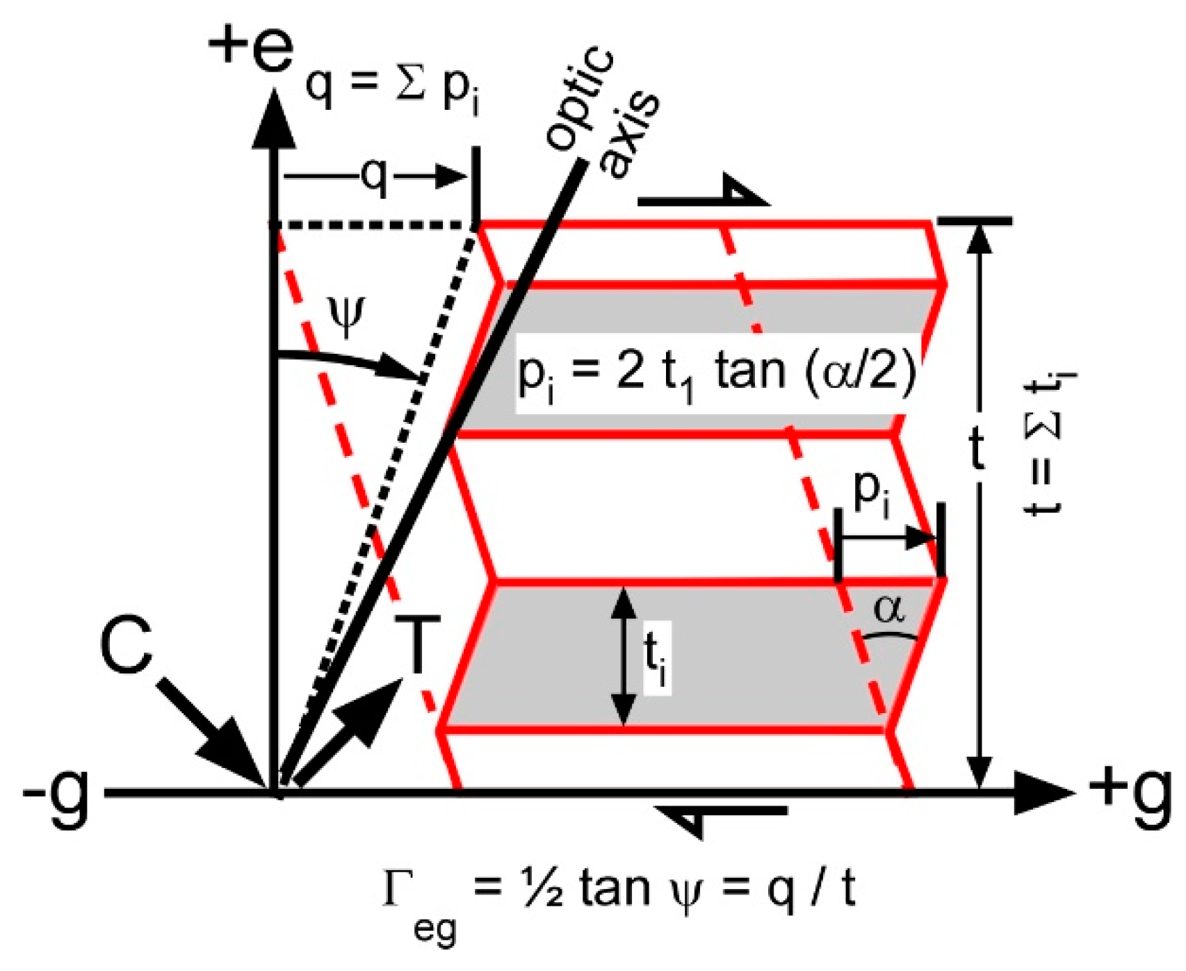
1] was the first to recognize that calcite twins in a partially twinned grain represent a measurable simple shear strain (
Figure 1). The amount of strain recorded by a twin set is a function of the number of twins, their widths, and the width of the grain in the direction normal to the twin plane. Each twin set is interpreted to represent an independent strain gauge embedded in the deforming rock. The engineering shear strain magnitude, the measure most commonly used by geologists, for a single twin set is tan ψ (
Figure 1), and the tensor shear strain is ½ the engineering shear strain [
4].
Once the strain is measured in a number of grains, the next question is how to combine this information to find the bulk strain tensor. Conel did a 3D tensor transformation on the strain in each twinned grain to bring the strain magnitudes all into the same (thin section) coordinate system. Then, he averaged each of the six tensor components, weighting the strain from each grain by the area of the grain. This produced strain tensors with magnitudes and directions that looked reasonable in the fold he studied.
Conel did the tensor transformation and averaging calculations by hand. When I began to use his strain technique it was then possible to use a computer. Researchers at Brown all had ready access to the university mainframe computer. To do a calculation, I wrote a program in FORTRAN, punched it into cards, submitted the cards, and then a day or so later the results, and the cards came back. Debugging the program was a very slow process. To validate the program, I decided to generate a synthetic data set. I produced a set of random twin orientations and, from an initial strain tensor, calculated the strain for each twin set in the deformed state. This was an error-free data set for which a correct calculation program would return the original strain magnitudes and directions. However, Conel’s calculation technique did not give the starting strain magnitudes or the orientations of the principal axes. Was this a programming error or something different?
The equation for the strain in a grain of a given orientation, Γ
eg, in the 3D tensor transformation equation has six components [
4]. After a week or two of perplexity, I realized that this represented one equation in six unknowns, which could be solved with measurements from multiple grains. As twinning alone does not cause or measure volume change, one unknown is eliminated by assuming constant volume. Thus, the equation could be solved uniquely with five equations from five differently oriented twin sets. With more twin sets, a best-fit solution can be found by multiple linear regression (least squares, for short), along with a statistical measure of the goodness of fit. The least-squares method finds the best-fitting strain ellipsoid for the twin-set strains in their measured U-stage orientations. The eigenvalues and eigenvectors of the result are the principal strain directions and magnitudes. The original strain tensor was obtained from the synthetic data by this calculation, proving that the least-squares approach worked and validating the computer program. This is the origin of the calcite strain gauge, the need to debug a complex computer program. (In 1994, Mark Evans brought the program into the desktop computer era and added the ability to plot the directional information on stereonets [
6]; see Tielke et al. in this issue for a new Excel version).
Forward modeling of randomly oriented potential twin sets produced grains with negative shear strain. This is exactly opposite to the shear direction shown in
Figure 1 and is impossible. By definition, the strain in a twin set can only be positive. In the initial modeling, grains with negative twin strains were simply discarded, but negative twin strains turned up later in the field data and would need to be explained.
Having error-free synthetic twinned grains made it possible to compare the different methods for interpreting the data. Comparisons were made to Turner’s dynamic analysis [
2], the Conel technique [
1], and a modified version of the Conel technique that Spang and Chapple developed [
7]. The overall result was that all three methods produce shortening and extension axes with roughly the same orientation, and the strain is substantially underestimated where magnitudes were available from Conel and modified Conel techniques.
Application of the strain gauge technique to field data produced new questions: First, how wide is a twin set? Under the microscope, thick twins have a measurable thickness of twinned material. Thin twins (formerly known as untwinned lamellae or microtwins), on the other hand, resemble dark lines crossing the grain. The field samples I was working with had many thin twins and a few thick twins. Conel [
1] had conducted a thorough analysis of the optics and concluded that the visible line was the result of an extremely thin twin. Therefore, the line represents a twin that is presumably equal to or thinner than the width of the line. Thick twins are bounded by lines of finite width, creating the question of whether the line width should be included as part of the twin thickness. The other question is whether or not the twin sets actually record the correct amount of strain. If twin sets are passive markers, each one should have exactly the correct strain for its orientation. However, at grain boundaries, where a twin set hits the adjacent grain, it might be prevented from deforming enough, causing the twin to underestimate the bulk strain. There might be other reasons that the twins under-record the strain. Neither the width nor accuracy questions can be definitively resolved using field data, but it was necessary to try.
In my field data, the ratio of thin twin-line thickness to actual twin thickness was the best fit by a ratio R = 0.5. A ratio of 0.75 made many thin twins thicker than thick twins, and a ratio of 0.25 generated too many very small-strain twin sets when compared to the simulated data. The inner thickness of the thick twins was used based on the premise that the black border was entirely an optical effect due to the abrupt change of crystal orientation. The accuracy of the principal strain magnitudes was guesstimated by comparing the strain calculated from twinning in a very gently folded bed close to an unfolded bed containing deformed brachiopods. The twin strain in the fold was taken as the average of the inner arc and outer arc values in order to average out the bending strain. The boundary-value strain for the fold is then the curved-bed shortening plus the internal strain. This latter concept was tested on a finite element fold model from Dieterich [
8] and matched to within 17%. The final strain for the outcrop fold was −3.6%, the brachiopod strain was −7.6%, and the shortening directions were 30° from one another. I concluded that the magnitude accuracy of the strain gauge should be no worse than a factor of 2. It is obvious that a large number of assumptions have been required to arrive at this point, leaving the accuracy of the strain gauge open to question. Consequently, I held off publishing my field results until 1975 [
9], after the experimental confirmation of the accuracy of the technique, discussed next.
3. Experimental Confirmation
I finished my dissertation in 1971 and published the strain gauge technique in 1972, but being unsure about the accuracy of the method when applied to real data, I held off publishing my results for the natural folds I had studied. After hearing a presentation of my results at a meeting, Mel Friedman and John Logan of the Texas A&M University Center for Tectonophysics group offered to let me try the method on thin sections from a series of experiments that John had run. In the experiments, cylindrical samples of limestone were shortened to axial strains of 0 to −8.4% (shortening negative). Then teaching at Syracuse University, I wrote and received a National Science Foundation grant to measure the samples and compare the strain gauge results to the experimental values. Later, after I became acquainted with John Logan personally, he told me that he and Mel had reviewed my grant proposal for the NSF and did not think the method would work but believed that I should be allowed to try it. This is an admirable mindset for grant reviewers, for which I thank them. The grant also helped to support an undergraduate research project by Larry Teufel at Syracuse in which he measured twin strain in a naturally deformed rock. Larry later studied at Texas A&M, where he ran additional experiments to further develop the strain gauge technique, as will be described later.
3.1. Methods
The experimentally deformed rock was the fossiliferous and spar-cemented Indiana limestone [
10]. Cylindrical samples were deformed at 100 MPa confining pressure, room temperature, and at a constant strain rate of 10
−4 per second. The actual porosity of the individual samples before deformation is unknown. On average, the undeformed limestone had a porosity of about 13%, which was reduced by the deformation to between 5.1% and 0.4%, depending on the sample. The load history began with the application of confining pressure, followed by axial shortening. Two samples were subjected only to confining pressure, which was applied to the side of the jacketed cylinder while zero displacement was maintained by the axial piston. This induced porosity loss, which caused twins to form. These samples provide insight into the effect of two-dimensional compaction. Six additional samples were first loaded laterally as described and then shortened using the axial piston.
As a side note, while preparing the current paper, I realized that the captions on
Figure 1 and
Figure 2 in my 1974 paper [
10] are reversed. That is confusing, even for me. As another side note, in my original papers, I spelled gauge as gage because that how is my first text on solid mechanics spelled it [
11] but changed to gauge when I saw that other geologists and rock mechanics generally spelled it that way.
The methods tested using the experimental data are the Groshong [
5] strain gauge technique, the original Conel [
1] technique, the Spang and Chapple [
7] modified Conel technique, and the then-new Spang [
12] numerical dynamic analysis method. All except the last method depend on the thickness of the twins. The Spang [
12] numerical dynamic analysis (NDA) method assigns a shear magnitude of 1 to every C and T axis, uses the tensor transformation law to transform all the data into thin-section coordinates, as did Conel [
1], and then averages the components. The eigenvalues and eigenvectors of this average tensor give the C (NDA
1) and T (NDA
3) axes plus the intermediate axis (NDA
2). One advantage of this method over contouring is that it forces the C and T axes to be orthogonal, which contouring of the axes on a stereonet does not necessarily accomplish.
3.2. Results
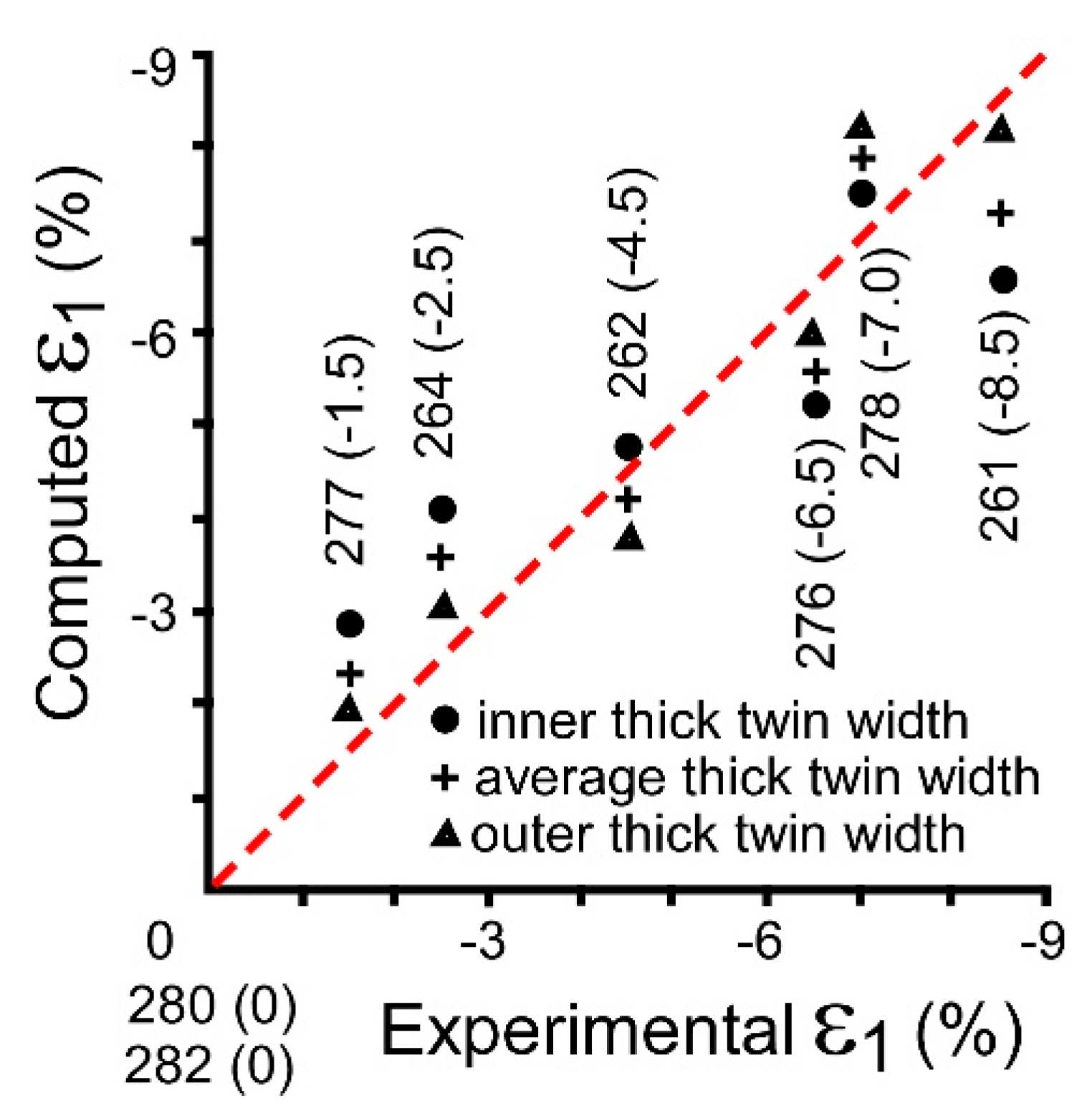
Due to the finite width of the twin boundary lines, alternative measures of twin width were again tested to find the values that best fit the experimental strain magnitudes (
Figure 2). The values that were selected, based primarily on the calculated statistical error, were the ratio R between measured and actual thin twin width of 0.5 and the inner width of the thick twins. In hindsight, today I might choose the outer thick twin width because it provides a better fit to the experimental strain magnitudes (
Figure 2). Note that the maximum strain magnitude difference is about 2. It seems unlikely, even today, that the difference between, for instance, 6.5% and 8.5% shortening would significantly impact any interpretive hypothesis. In a later series of experiments Teufel [
13] found that the strain gauge calculation consistently slightly underestimated the experimental strain magnitude, another reason to slightly increase the thicknesses assigned to thick twins and perhaps even to the thin twins.
Two representative samples will be discussed in detail; sample 282, which underwent only lateral compaction, and sample 278, which underwent a large axial shortening in addition to lateral compaction. Sample 282 gives the clearest picture of the effect of two-dimensional compaction because its porosity was reduced to almost zero (0.8%) by the initial loading. Even though the axial displacement is zero, this form of loading produces a deviatoric extension in the axial direction because of the lateral shortening due to porosity loss. The strain gauge technique indicates a deviatoric extension with an axis about 10° from the cylinder axis (
Figure 3a), a fairly accurate estimation of the direction. The deviatoric extension magnitude is +1.3%. This is comparable to the experimental value, which could be as much as +4.3% depending on the exact initial porosity, which is unknown. The Turner [
2] dynamic analysis extension axis distribution (
Figure 3a) appears to be random, and the compression axes are equally random [
10]. Even though grains are clearly deformed by twinning, there is no obvious directional information given by the Turner technique. The numerical dynamic analysis (NDA) locates a deviatoric extension axis (NDA
3) within about 20° of the cylinder axis, a reasonable approximation, given that the T axes appear to be random.
Sample 278 is one of the most deformed, having an axial shortening of −7.5%. The computed strain gauge maximum shortening direction is within about 2° of the experimental direction, and the computed strain magnitude is just 0.5% larger than the experimental value, a very good match. For this sample, Turner compression axes show a clear clustering around the cylinder axis (
Figure 3b) and the extension axes form a girdle perpendicular to the cylinder axis (see [
10]). NDA
1 (average C axis) is also almost exactly parallel to the cylinder axis. The NDA
1 magnitudes are 0.5% or less (Figure 4a) and do not correlate with either the stress or strain magnitudes.
The twinning strain gauge does not measure volume change, therefore the calculated strains represent the deviatoric component of the total. For deviatoric strain, two principal strain magnitudes must have one sign and the third will have the opposite sign because the sum of the three must be zero. The odd-signed axis is always the best located in the experiments because of the cylindrical symmetry of the strain; it is in the direction of the cylinder axis. In the experiments, the same-signed axes should be identical in magnitude, and therefore their directions are not well constrained.
3.3. Noise Reduction
Noise is defined as (1) the size of the statistical standard error [
5], (2) a negative expected value for the strain of a twin set as calculated from the best-fit result [
10], and (3) the size of the difference between the expected value for each twin set and the twin strain, as calculated from the best-fit result [
10]. Potential sources of noise can include measurement error, inhomogeneous strain, or a complex strain history. My 1974 experimental results were considerably “noisier” than the results from my field data, a fact that needed an explanation.
Can the sources of the noise be identified and then reduced using methods that will also work with field data? In 1974 [
10], I inferred that much of the experimental noise probably resulted from inhomogeneous strain due to porosity collapse. This was later confirmed experimentally by Teufel [
13] who, using the same material (Indiana limestone), obtained much less noisy results by not including twin sets associated with porosity collapse. These grains were identified as ones where the twins start at grain boundaries but do not continue across the whole grain. This criterion had been put forward by Friedman [
14] and was applied by Teufel [
13]. Grains similar to this were included in the data sets in my 1974 paper, none of which was recorded, making later removal impossible.
Removing the largest deviations with respect to the expected values worked well with my 1974 experimental data. This cleaning technique should remove significant measurement errors and reduce the effect of an inhomogeneous strain. Removing the 10% largest deviations seemed to provide a reasonable balance between removing inconsistent measurements but without eliminating too much of the hard-won data [
10]. This strategy also worked well for experiments by Teufel [
13] and Friedman et al. [
15].
Negative expected values pose a different kind of problem. Negative expected values indicate the wrong sense of shear for the orientation, indicating a grain that should not be twinned given the calculated strain tensor. Results in my 1974 paper [
10] show that some negative expected values can arise from inhomogeneous strain. It seems unlikely that the strain would be perfectly homogeneous throughout every grain in every direction. Each grain has only three directions in which it can deform by twinning, and adjacent grains must provide some resistance to the formation of twin sets that try to deform a boundary that is not suitably oriented to twin. Thus, some twin sets with small negative expected values are no surprise, even in rocks with no initial porosity. However, large numbers of negative expected values would seem to imply a different process.
6. Stress or Strain?
There has long been a tendency to refer to dynamic analysis [
2] and related techniques as stress analysis, whereas methods using measured twin widths are referred to as strain analysis. I suggest that, if you can visually detect it, it is strain. For natural deformation, stress must be calculated from the strain, and that requires knowing the appropriate flow law and its physical constants. As shown previously, almost any reasonable calculation or contouring technique will provide a good estimate of the odd-signed strain axis direction, equivalent to the corresponding stress axis if the strain is irrotational. Two different approaches for obtaining stress magnitude from twinned calcite are discussed next.
The standard approach to finding the stress magnitude from strain is via the appropriate flow law. The stress–strain relationship for the experimentally deformed samples from 1974 is given in
Figure 4a. The relationship is probably nonlinear, but a straight-line best fit is shown. The NDA
1 values are not correlated to the strains but are most likely related to the strength of the C and T axis concentrations. The twin strain calculated by the strain gauge technique is well correlated to the stress except for the largest strain value. Here, the twin data have had the 10 largest deviating twin sets removed from the calculation. This improves the agreement between the experimental and calculated values by a small amount except for the maximum strain magnitude, which remains underestimated. This is another reason why it probably would have been better to use the outer thick twin width in the calculation (
Figure 1). The stress–strain relationship in
Figure 4a is not predictive for field use unless the flow law is identical to that in the experiments.
After finishing my 1974 paper, I passed the thin sections along to Jamie Jamison and John Spang at the University of Calgary. As part of his MSc thesis, Jamison developed a very different approach to estimating stress magnitude. The basic concept is that, because there is a critical resolved shear stress required to initiate twinning, in a randomly oriented crystal aggregate the greater the differential stress applied to the aggregate, the greater the number of twin orientations that will be activated. Jamison and Spang [
17] derived a relationship between the expected percentage of twinned grains and what they termed the resolved shear stress coefficient, S
1, which is a function of the angles between the pole to the twin plane, the glide direction, and the principal stress directions.
Figure 4b is a plot of the percentage of grains having one, two, and three twin sets. These percentages are measured on a thin section and plotted, giving the value of S
1 for that sample. S
1 is converted to stress with the equation Δσ = t
c/S
1, where t
c is the critical resolved shear stress for twinning. They used a value for t
c of 10 MPa based on the research by Turner, Griggs, and Heard [
18], and Friedman [
19].
I have plotted the Jamison and Spang measurements [
17] for their samples in
Figure 4b. For an internally consistent result, the cumulative percent of one, two, and three twin sets for a thin section should fall on a vertical line. The relationship between Δσ and S
1 is strongly nonlinear, with Δσ going to infinity as S
1 goes to zero. Thus, the resolution of Δσ using the graph as presented is not very good for S
1 < 0.1, equivalent to Δσ > 100 MPa. For the two least deformed samples (264, 262), the lines are close to vertical and the predicted stresses are very close to the experimental values. The other samples provide stress estimates that are too high. The worst fit is the most deformed sample (261) for which the line between two and three twin sets is the farthest from vertical and the stress estimate is significantly greater than the experimental value (the strain gauge result for this sample (
Figure 4a) is the biggest underestimate of the strain magnitude). The curve for three twin sets (
Figure 4b) yields the most accurate result, as noted by [
17]. Using the three twin-set values, the predicted maximum compressive stress in every sample agrees with the experimental value to within 30 MPa.
The stress–strain relationships in
Figure 4a,b may be misleading as estimates of the stresses in naturally deformed rocks because the results depend on the load history. The experiment was conducted at a constant strain rate, which causes the stress to increase with time under the given conditions of temperature and pressure. As noted by [
17], Friedman and Heard [
20] found that the number of twins and the number of twinned grains increases with time at constant differential stress in a creep (constant stress) test. The effect of the loading rate on the stress and twin strain, along with the temperature and pressure effects, should be investigated carefully before any attempt is made to infer stress magnitudes from twin strain.
7. Discussion
It is now possible to discuss the interpretation of a representative fold from the group of natural folds that I originally studied [
9]. The example in
Figure 5 is selected because it is the best geometric match to the finite-element fold model of Dieterich [
8]. The values of shortening at corresponding locations in the natural and model folds differ by an order of magnitude or more. My initial conundrum was whether or not the calculated strain could be incorrect by such a large amount. The experimental results show that the strain gauge calculation is accurate to 20 or 30% of the magnitude value; thus, the order-of-magnitude discrepancy is real. This is also consistent with the fabric of the limestone itself because the fossils are not obviously deformed, indicating that the maximum shortening at the grain scale is almost certainly no more than 10%.
Two additional deformation mechanisms are obvious in the fold (
Figure 5): tension fractures, now filled with secondary calcite, and wavy stylolites containing insoluble residue of quartz, dolomite and, in some, presumed organic material. Stylolites are abundant throughout most of the layer but cannot be positively identified near the top because there the layer consists of fine-grained dolomite without fossils. The number of stylolites shown is the minimum because zones of insoluble residue that do not clearly truncate a fossil are not included. The stylolites are roughly normal to the measured shortening directions and to the predicted shortening directions in the model. Some stylolites curve toward bedding in the outer arc in both the anticline and in the right-hand syncline, as predicted by the model. The filled tension fractures at the top and base of the layer represent outer-arc extension. The large fracture on the right limb of the anticline initiated at its lower, most nearly horizontal boundary and opened obliquely with a left-lateral sense of shear, as indicated by the fabric of the calcite filling [
9]. The fracture orientations are parallel to the predicted maximum compressive stress directions in the buckle fold model [
22]. All three deformation mechanisms are contemporaneous. The strain is partitioned among them according to their individual flow laws and each has a different effect on the final geometry. Presumably, only a small fraction of the total strain is partitioned into calcite twinning with most of the strain being by pressure solution. Duplicating the results in
Figure 5 is a worthy challenge for anyone conducting mechanical modeling.
New rock deformation tests could answer many questions. Each new experiment will provide the opportunity to use every calculation technique now available to observe how they compare. A high priority should be to find out whether constant-stress (creep) experiments produce the same twin strains as constant strain rate experiments. The results should show whether or not stress magnitudes can be predicted from the twin strain. It would also be of interest to see if the final fabrics differ between creep and constant strain rate experiments at the same total strain. All experiments should be run in both wet and dry conditions to investigate whether water affects the strain partitioning.
Natural and human-made compaction is a significant issue in reservoir development for areas ranging from hydrocarbon production to waste disposal, to potable water production. Calcite twin strains might provide new insights into the process. Experiments should begin with uniaxial compaction tests, representing compaction due to the weight of the overburden. Is it possible to distinguish between natural compaction and human-made compaction? Twins that do not cross an entire grain are thought to indicate the collapse of adjacent pores. What would happen if the strain for only such grains is calculated?
There are a variety of other interesting questions that could be addressed experimentally. For example, how critical is the magnitude of the difference between the principal strain magnitudes? This could be examined with true triaxial experiments in which the three principal strains can be controlled independently. It would also be interesting to see the results of the deformation of samples with a strong initial crystal-orientation fabric. Can the imposed strain be accurately measured or does the rock fabric prevent it? I hope someone finds one or more of these suggestions of interest and takes action.

