Article

The Hydrothermal Vent Field at the Eastern Edge of the Hellenic Volcanic Arc: The Avyssos Caldera (Nisyros)

by
Ana Dura
1,*,
Theo J. Mertzimekis
2,
Paraskevi Nomikou
1,
Andreas Gondikas
1,
Martín Manuel Gómez Míguez
2,3,
Evangelos Bakalis
4 and
Francesco Zerbetto
4
1
Department of Geology and Geoenvironment, National and Kapodistrian University of Athens, Zografou Campus, GR-15784 Athens, Greece
2
Department of Physics, National and Kapodistrian University of Athens, Zografou Campus, GR-15784 Athens, Greece
3
Departamento de Astrofísica, Universidad de La Laguna, E-38200 La Laguna, Tenerife, Spain
4
Dipartimento di Chimica “G. Ciamician”, Università di Bologna, 40126 Bologna, Italy
*
Author to whom correspondence should be addressed.
Geosciences 2021, 11(7), 290; https://doi.org/10.3390/geosciences11070290
Submission received: 22 April 2021 / Revised: 2 July 2021 / Accepted: 8 July 2021 / Published: 13 July 2021
(This article belongs to the Special Issue Present and Past Submarine Volcanic Activity)

Abstract

:
Almost three-quarters of known volcanic activity on Earth occurs in underwater locations. The presence of active hydrothermal vent fields in such environments is a potential natural hazard for the environment, society, and economy. Despite its importance for risk assessment and risk mitigation, the monitoring of volcanic activity is impeded by the remoteness and the extreme conditions of many underwater volcanoes. The morphology and the activity of the submarine caldera, Avyssos, at the northern part of Nisyros volcano in the South Aegean Sea (Greece), were studied using a remotely operated underwater vehicle. The recorded time series of temperature and conductivity over the submarine volcano have been analyzed in terms of the Generalized Moments Method. This type of analysis can be used as an indicator for the state of activity of a submarine volcano. Here, we expand the work conducted for the first time in 2018. We present the findings of the geological exploration and the mathematical analysis, obtained from the data collected in October 2010. The temperature and conductivity time series show minor fluctuations in a rather stable environment. Based on these results, the impact of developing appropriate mechanisms and policies to avoid the associated natural hazard is expected to be important.

1. Introduction

The Hellenic Volcanic Arc (HVA) resulted from the northward subduction of the African plate underneath the active margin of the European plate [1,2,3,4]. The HVA extends from volcanic centers of the Saronic Gulf in the west (W) to the Kos–Nisyros Complex in the east (E) [5,6].
The HVA volcanoes have been especially active in the Late Pleistocene–Holocene and occur onshore [7,8,9] the peninsula of Methana and the islands of Poros, Milos, Santorini, Kos, and Nisyros [10], as well as offshore [6], with several submarine volcanoes detected in the Epidauros Basin in the W Saronikos Gulf [11,12,13] NE of Santorini, the submerged Kolumbo Volcano [14,15,16,17], and in the submarine area around Nisyros [18,19,20,21,22,23,24,25,26,27] (Figure 1).
Volcanism related to the modern South (S) Aegean volcanic arc in the Kos-Nisyros area began in Pliocene times [10,28]. Moreover, in Plio–Pleistocene times, lavas were emplaced on the centers of Pachia and Perigusa (a few km W of Nisyros) and in the lower succession of Nisyros [29,30,31]. In Quaternary times, major magmatic activity in the area led to the eruption of the Kos Plateau Tuff, which covers an area of more than 3000 km 2 . The Plateau is thought to have been produced about 160 ka from a volcanic source located between Kos and Nisyros, with its center close to the young volcanic island of Yali [30,31,32,33,34,35,36,37]. According to Pe-Piper et al. [38], the Kos Plateau Tuff was erupted from an original andesite stratocone, the remnants of which are present beneath Yali, Nisyros, and Pachia. The center of this eruption is not known with accuracy, but it is probably located in the submarine area, north of the Yali islet, a few kilometers NW of Nisyros [21,25].
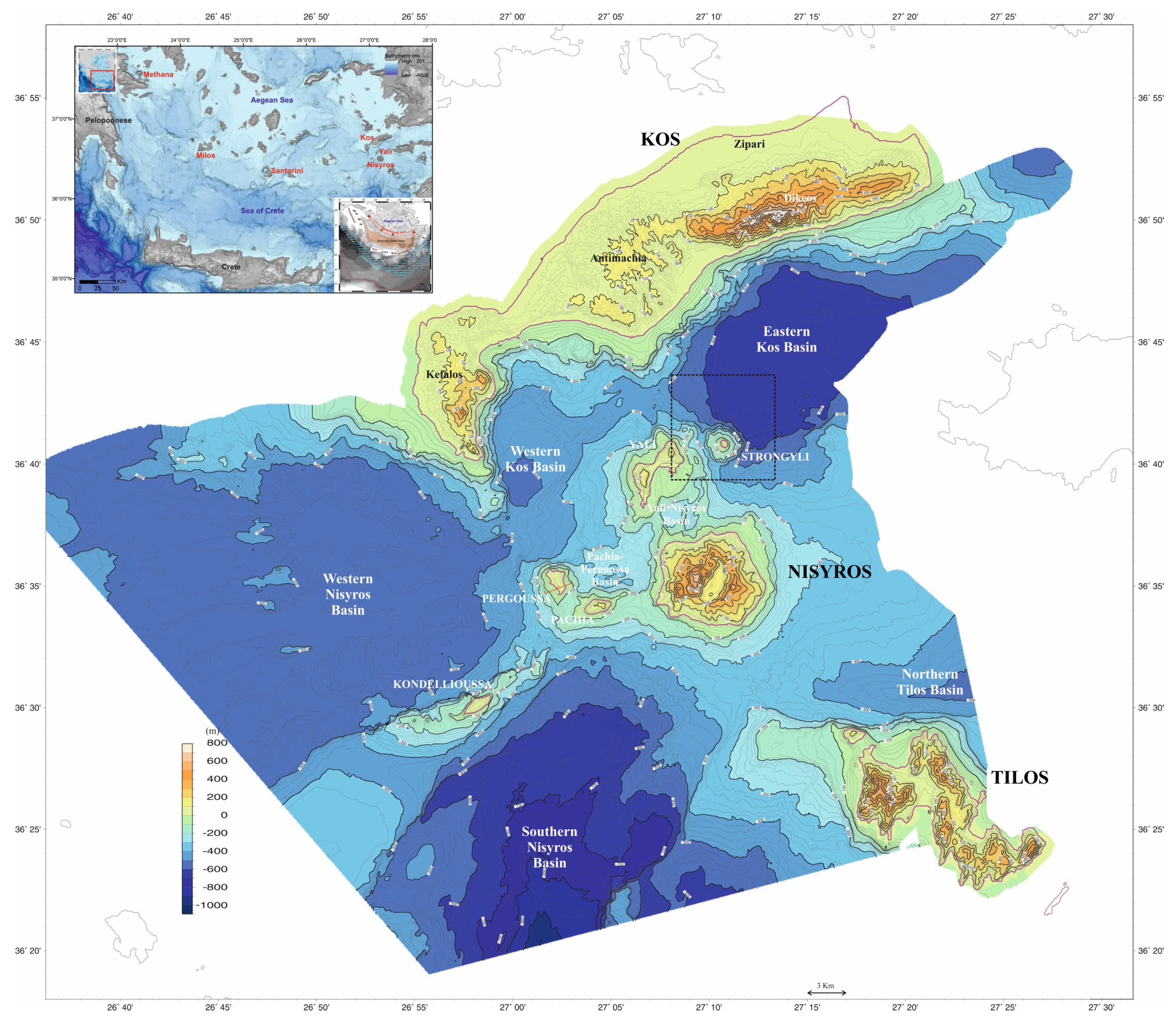
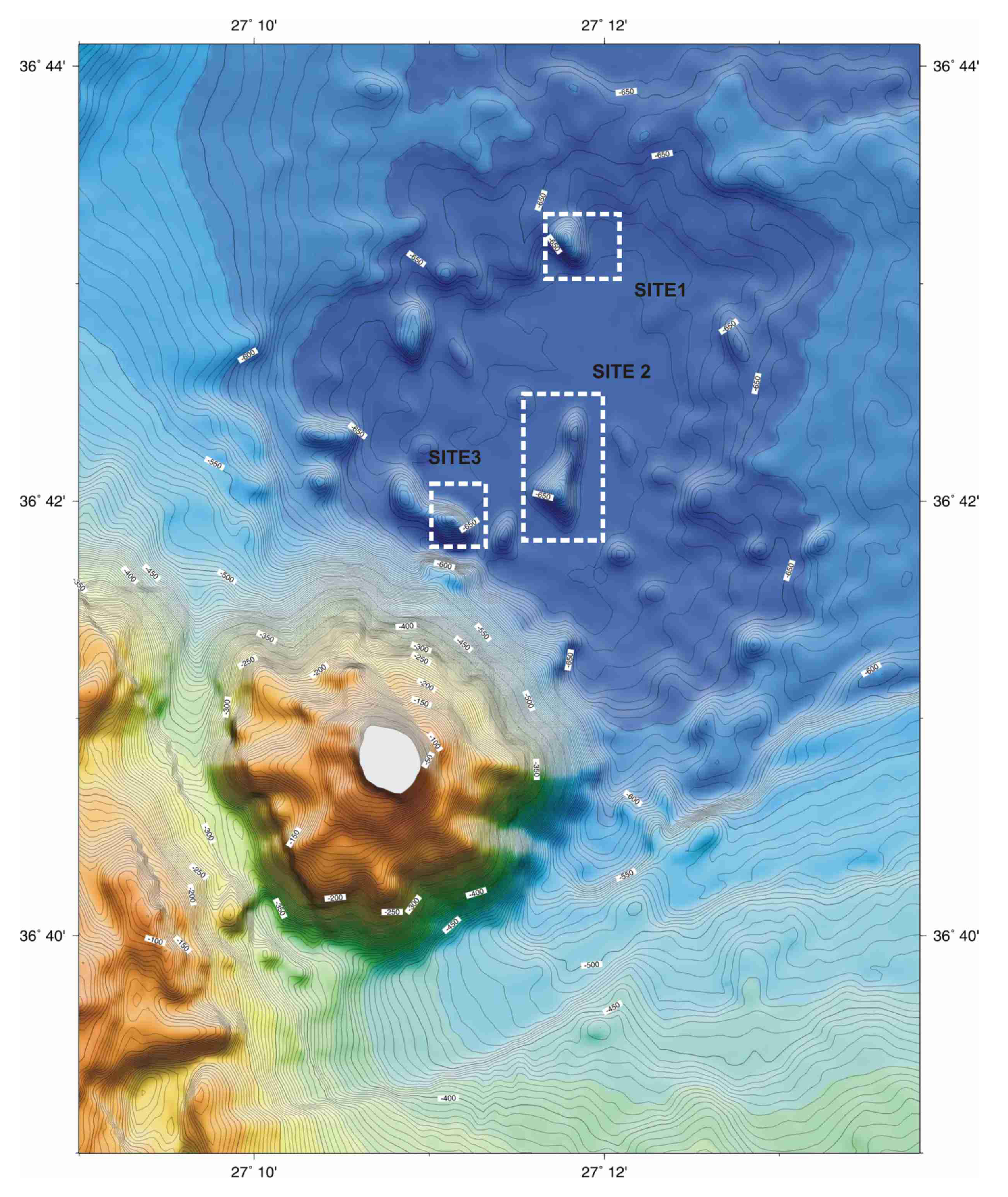
The main onshore morphological features of the Kos-Nisyros-Tilos volcanic field are three zones of positive relief comprising Kos in the NW (843 m elevation in Mt. Dikeos), Nisyros (698 m in Mt. Prophitis Ilias) and surrounding islets in the middle, and Tilos (654 m, Prophitis Ilias) in the SE [23,24]. These zones divide the submarine area between Kos and Tilos into two basins with an average sea bottom depth of 600 m. Consequently, the topographic differences between the mountain ranges and the submarine basins are of the order of 1–1.5 km. This results in very steep slopes and a narrow zone of shallow depths (0–300 m) in the S coast of Kos Island. By contrast, the area of the islets around Nisyros is characterized by extended shallow water depths [21,26,39] (Figure 1).
Volcanism developed in the marine area around Nisyros with the formation of individual volcanic centers, each of them exhibiting a special geometry and evolutionary stage [19,21,23,24,26]:
(i)
The Nisyros Volcano, which is exclusively made of Quaternary volcanic rocks and has been characterized by a stratovolcanic cone, whose eruption created the Nisyros caldera. The largest present-day phreatic crater of Stephanos occurs within the Nisyros caldera along with other phreatic craters (such as Alexandros, Polyvotis, Phlegethon, and Achelous) that are still emitting fumaroles.
(ii)
The Yali volcano, which exhibits a partly submerged caldera. The two parts of Yali are dislocated by a postcaldera N–S fault. Western Yali is made of two successive pumice formations, whereas Eastern Yali is made of obsidian glass covered by a pumice formation (equivalent to the upper pumice of the Western Yali).
(iii)
The Strongyli volcanic cone, which starts at a −600 m depth (sea-bottom) and reaches +120 m at the top of the present day Strongyli Islet, where a 300 m-diameter volcanic crater is observed (pre-caldera stage).
(iv)
The Pergousa volcanic cone, which is made of stratovolcano type formations, with alternating lava flows and pumice layers (pre-caldera stage).
(v)
The volcanic domes of Pachia Islet and the submarine volcanic domes to the E of Kondeliousa Islet.
No volcanic activity is documented on the island for at least 25 ka after the formation of the volcanic domes of Prophitis Ilias; the only reported historical explosions are related to the formation of several phreatic craters inside the caldera. Violent earthquakes, gas detonations, steam blasts, and mudflows accompanied the most recent hydrothermal eruptions in 1871–1873 and 1887 AD (see the work in [10] and references therein). During this activity some people were injured and minor damages were caused to the infrastructures.
The crustal seismicity of Nisyros exhibits the basic properties of active volcanic regions in quiescent periods [40]. Nisyros’ seismicity has shown episodic unrest with local swarm-like earthquake sequences separated by months and years of quiescence. This is a characteristic which makes Nisyros comparable to other large calderas, such as Campi Flegrei (Naples, Italy), Rabaul (Papua, New Guinea), Yellowstone (WY, USA), and Long Valley (CA, USA) [41]. At the end of 1995, the Nisyros volcanic region entered an episodic unrest period with long-lasting, highly clustered earthquake activity, which seems to be a characteristic of the region rather than a precursor of a volcanic eruption [40].
From 1996 to 1998, the island experienced an episode of unrest that included a series of shallow earthquakes up to a M = 5.5 magnitude [40], a considerable temperature increase in the hydrothermal system [42], and ground deformation [43]. Seismic activity related to the Mandraki fault caused significant damage on the island along the W edge of the town of Mandraki (located in NW Nisyros) [26]. The fault extends N under the sea.
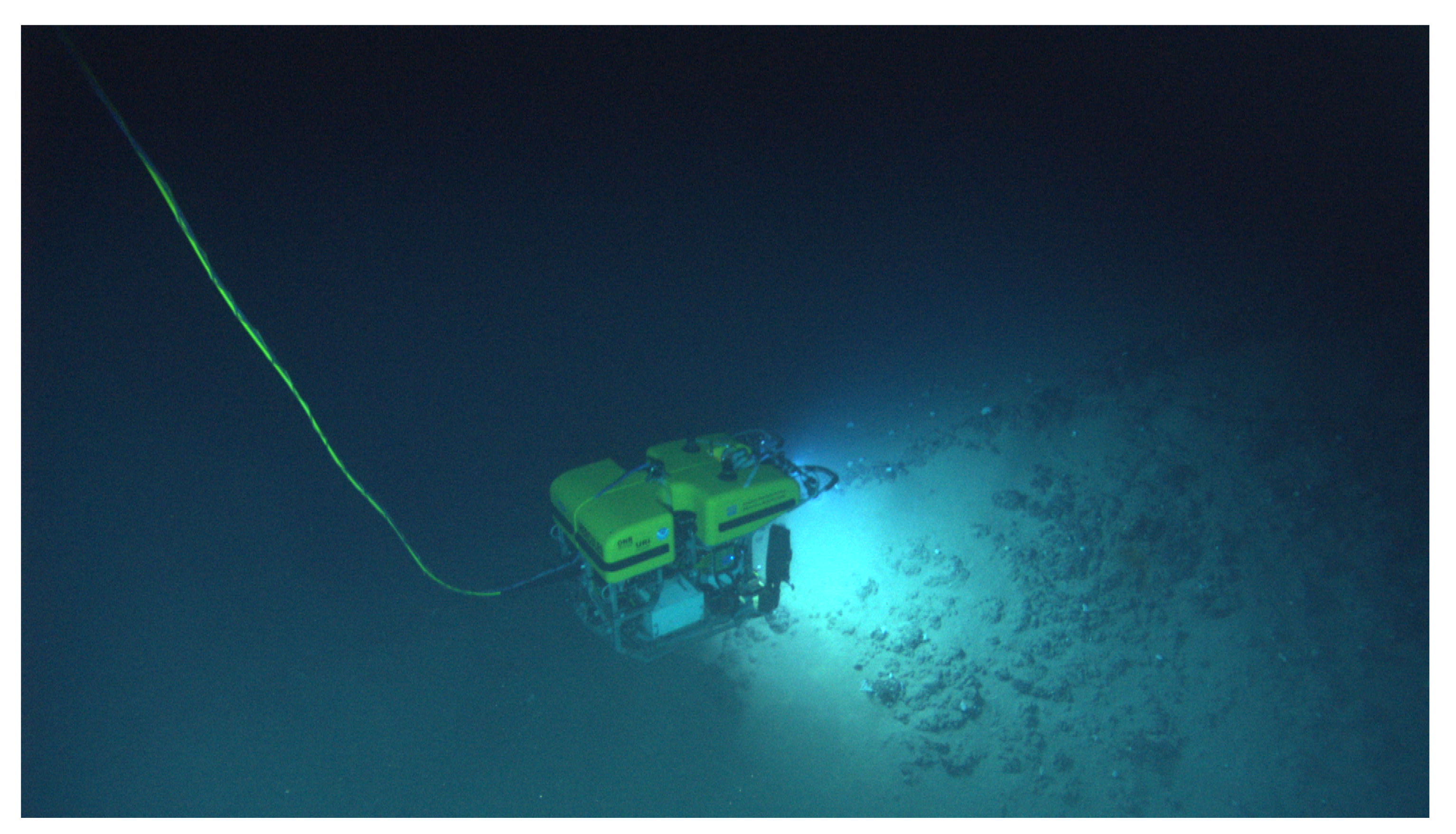
Despite its importance for risk assessment and mitigation, monitoring of the activity of submarine volcanoes is impeded by the remoteness and the extreme conditions of underwater volcanoes [44,45]. An efficient method to study those characteristics is to employ sensors aboard Remotely Operated underwater Vehicles (ROV), able to record CTD data (Conductivity, Temperature, Depth) in the water column (see, e.g., in [46]). Previous studies of the underwater features around Nisyros have focused on the geomorphology, using ROV to collect data, and have explored the volcanic field offshore, mainly in the Nisyros-Yali-Strongyli area [26].
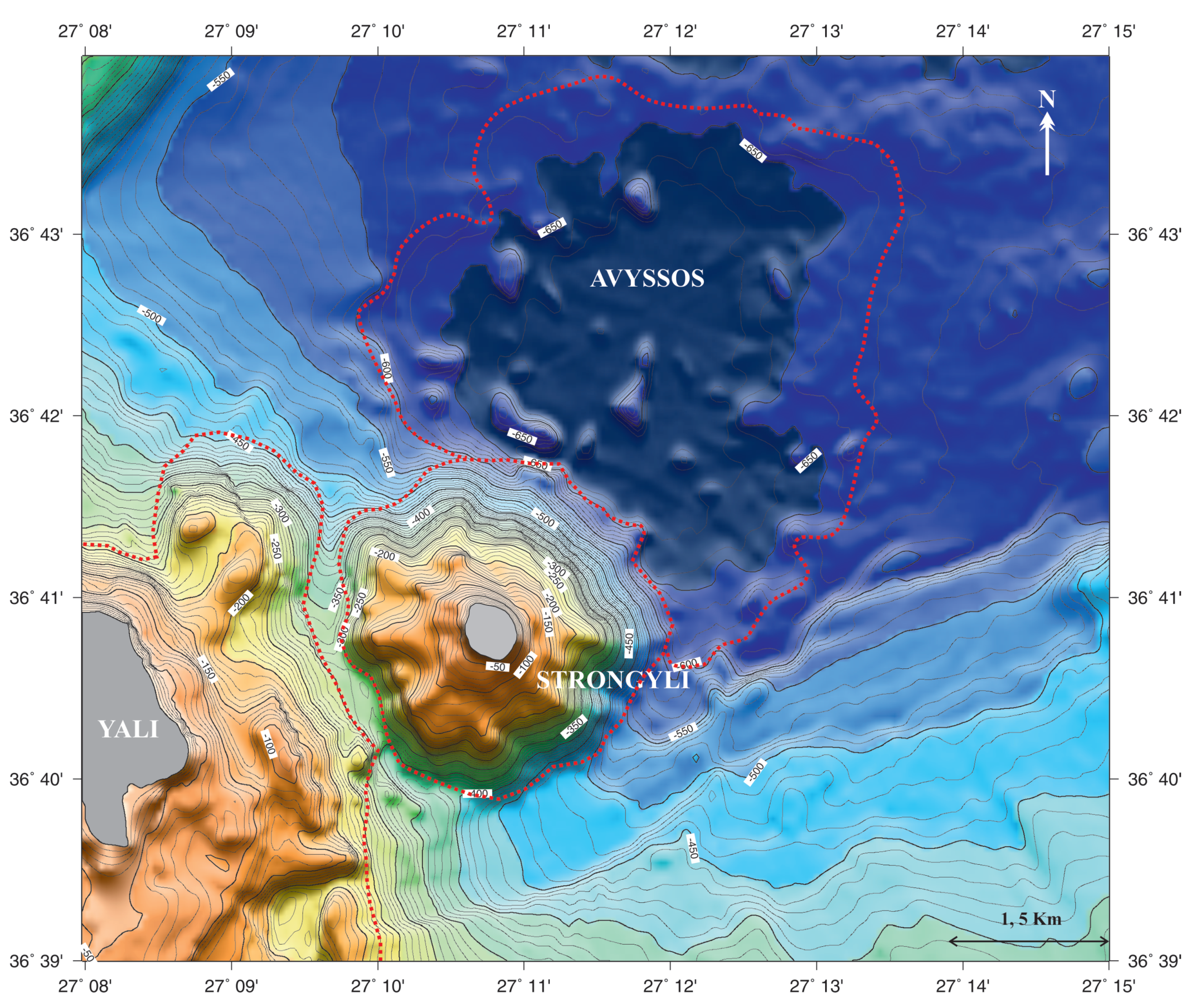
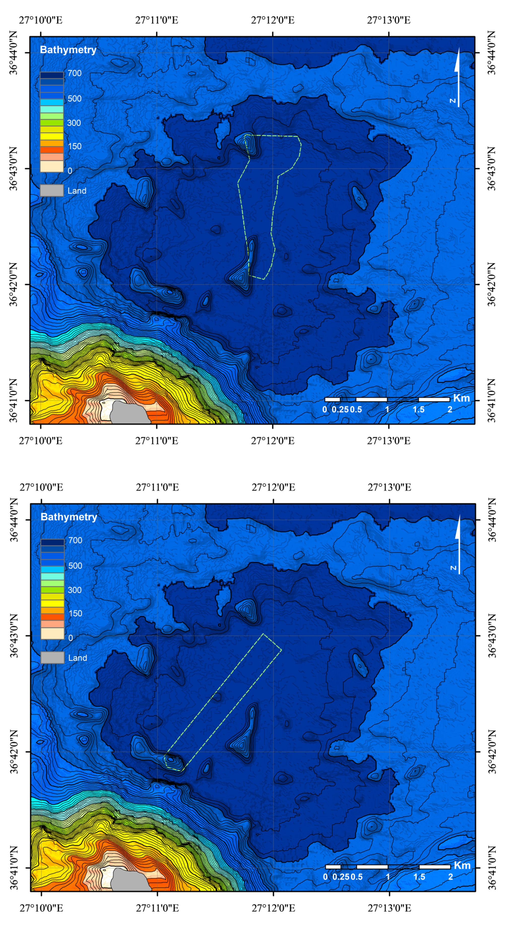
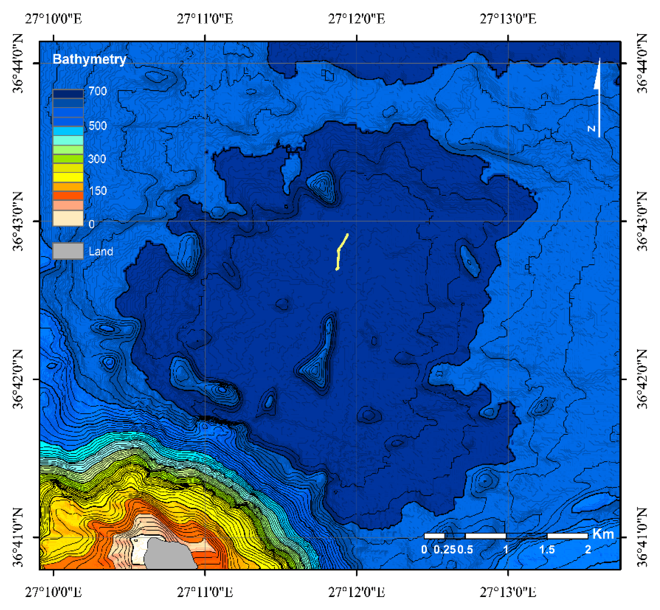
Such data were collected for the first time in the underwater caldera Avyssos at the NE part of the volcanic islet of Strongyli, N of Nisyros volcano (Figure 2). The size of Avyssos caldera stretches for 3 km and 4 km along NW-SE and NE-SW directions, respectively, with a maximum depth of 680 m [23,24]. In addition, there is an underwater hill, about 1 km long at the center of Avyssos with a positive relief of about 60–70 m above a flat sea bottom. A dedicated mission conducted in 2010 focused on exploring the unknown volcano-tectonic characteristics of the Nisyros-Yali-Kos region and the associated volcanic field around Nisyros [26]. The main focuses of that mission included the observation of the previously unexplored hydrothermal field of Avyssos. In the present work, results from the full investigation are reported for the first time in terms of high-frequency CTD measurements using sensors mounted on a ROV (Figure 3).
A small portion of the full data set has been reported and analyzed by our group in [47] using a novel mathematical method, based on the Generalized Moments Method (GMM) [48]. The same modeling method had been successfully applied to identify the underlying stochastic processes driving the activity of the Kolumbo volcano in the Aegean sea [49]. This study yielded interesting aspects of the underlying dynamics of Kolumbo’s hydrothermal vent field during rest and unrest periods.
Due to the non-zero probability of eruption, and thus of its potentially devastating effects on the environment, society, and economy, the dynamic state of Avyssos is studied utilizing the data collected in October 2010, significantly extending our initial work in 2018, as reported in [47], to the full hydrothermal vent field in Avyssos.

2. Materials and Methods

2.1. Data

Recent multibeam mapping and seismic profiling have revealed several previously undetermined features near Nisyros and Yali, including a number of submarine volcanoes located NE of the Strongyli islet. The ROVs Argus and Hercules were deployed from E/V Nautilus in October 2010 to explore the slopes of the crater and the volcanic domes identified on the bathymetric map acquired from the multibeam data (Figure 2).
The CTD sensor was a calibrated SeaBird FastCAT 49Plus CTD probe mounted on ROV Hercules (Figure 3), which was tethered to ROV Argus receiving power from the ship and transferring data via a fiber-optic cable. During dives, the CTD sensor continuously acquired data at a rate of 16 Hz [50]. All data used in the mathematical analysis described in Section 2.2 were recorded at the deepest possible locations inside the Avyssos caldera. These CTD data sets from Nisyros/Avyssos are presented for the first time in literature.
The precise position of the vehicle was measured by highly calibrated pressure sensors on the vehicle. Argus is the tow sled that hung directly beneath the operating vessel and helped reducing ship motion effects from the hovering of Hercules over the seafloor. This vessel additionally provides working lights and “birds-eye” views for Hercules, which was used to gather the images from the seafloor during the mission (Figure 4, Figure 5 and Figure 6).
The main data collected were conductivity, temperature, and depth, as well as salinity and sound velocity. Vertical (depth) profiles and times series have been reconstructed from the raw data. In the following paragraphs, the focus of analysis is on temperature and conductivity, which are directly measured by the mounted sensors, as in the case of earlier applications [46,47,49].

2.2. The Generalized Moments Method

In recent works, a novel mathematical approach based on the GMM has been applied to study the underlying mechanism driving the CTD times series in two cases: the first recorded over a very active submarine hydrothermal vent field (Kolumbo, Santorini) [49], and the other recorded over a less active area (Nisyros caldera) [47]. Details of the method are presented in those references, where the reported results have also established the validity of the novel approach. In the next few paragraphs, a brief overview of the method is given.
Hydrothermal vent activity may be detected by measurements of the physical and chemical properties of the fluid, obtained from CTD depth profiles and time series. Such a sequence of events (measured property versus time) can be (generally, but not necessarily) assumed as a manifestation of a stochastic process. A first estimate of the behavior of a stochastic process, x ( t ) , can be made in terms of its variance. For discrete data time series, by taking the time average, the variance reads
W ( T , Δ ) = 1 M i = 1 M 1 T Δ n = 1 T Δ ( x i ( n + Δ ) x i ( n ) ) 2 1 M i = 1 M 1 T Δ n = 1 T Δ ( x i ( n + Δ ) x i ( n ) ) 2 K γ Δ γ
where M is the number of experiments repeated under the same conditions, to express the ensemble averaged over all records, whereas for M = 1 , the first summation is omitted. T is the length of the recorded trajectory, and Δ is the lag time, which is the elapsed time between any two measurements and plays the role of time for discrete data sets. K γ is a generalized coefficient expressed in proper units. It can serve as a tool for a first classification of the stochastic process based on the value of the exponent γ . A stochastic process is classified as sub–normal or antipersistent for 0 < γ < 1 , Brownian or normal under certain conditions for γ = 1 , super-normal or persistent for 1 < γ < 2 , ballistic for γ = 2 , and stationary for γ = 0 . Furthermore, n = 1 , 2 , , T Δ and Δ = τ , 2 τ , , τ m a x τ [51].
More insights on the mechanisms governing a stochastic process can be extracted by using sophisticated methods appropriate for time series analysis [48,52]. Among them, the GMM, which has been successfully applied in numerous fields, is robust and works well even for short time series [53,54].
Considering a discrete time series in the form x ( n ) with n = 1 , 2 , , N , where N is the total number of steps (measurements), and if the minimum lag time defined as the reciprocal of the sampling rate, f, or in other words the time elapsed between two consecutive measurements, is τ , then the total length of the trajectory is T = N × τ . In brief, the “recipe” works as follows:
(1)
Construct time series with different lag times.
(2)
Estimate the statistical moments (Equation (2)).
(3)
Show that moments scale according to Equation (3).
In more detail, we create new time series, y n ( Δ ) = ( x ( n + Δ ) 2 x ( n ) 2 ) 1 / 2 , then we estimate the moments of the time series according to
ρ ( q , Δ ) = 1 T Δ n = 1 T Δ ( y n ( Δ ) ) q
where even fractional values of the moment, q, are taken into account. Note that we use only positive values of the moments. The values of the moments in the range 0 < q 2 are responsible for the core of the probability density function (pdf), whereas higher moments, q > 2 , contribute to the tails of the pdf.
In general, the moments scale according to Equation (3), in which z ( q ) is the structure function whose shape gives information on the stochastic mechanism(s) governing the motion.
ρ ( q , Δ ) Δ z ( q )
When the structure function takes the simple form z ( q ) = H q , there is a direct relation between γ and the co-factor of the structure function, namely, γ = 2 H , where H is the Hurst exponent [53]. If z ( q ) is a linear function of q or is linear in different portions (bilinearity), then the mechanisms that likely govern the stochastic sequence are additively decomposable. The linear dependency of z ( q ) on q describes monofractal processes. Instead, if z ( q ) has a convex shape as a function of the order of the moment q, then multiplicative processes drive the stochastic sequence. This also implies that H is a function of q. For some values of q, the exponents H ( q ) = z ( q ) / q are associated with special features. For q = 1 , the value of H ( 1 ) describes the scaling behavior of the absolute value of the increments and is identified with the Hurst exponent if the process is monofractal. For q = 2 , the value of H ( 2 ) is associated with the scaling exponent of the autocorrelation function and is related to the power spectrum [55]. Of all types of multifractals, universal multifractals are likely to be ubiquitous [56,57], and the structure function reads [54]
z ( q ) = H q C a 1 ( q a q )
For a = 1 , Equation (4) takes the form z ( q ) = H q C q l o g ( q ) , and the distribution diverges from a Cauchy–Lorentz distribution. For a = 2 , Equation (4) reads z ( q ) = H q C ( q 2 q ) , and the distribution diverges from a lognormal distribution.
In the present study, the GMM is performed on the temperature and conductivity time series recorded over the hydrothermal vent field of Avyssos. As the ROV hovers over the extended hydrothermal vent field along various tracks, the time series present a variability in locations on the horizontal plane. All measurements considered in the analysis presented below have been carried out near the seabed, directly above the vent sources, which despite being weak, are ostensibly active, and present anomalies in the CTD depth profiles (temperature and conductivity). The ROV hovering motion (<1 m/s) perturbs the exact nature of the mathematical formalism, but it has been considered a safe approximation due to the widespread, overall homogeneous, vent activity along the studied tracks and the very slow horizontal translation. The results from the application of the method are reported in the next section.

3. Results

3.1. Mapping

CTD data were collected in Avyssos between October 10 and 12 2010 at a 16 Hz sampling rate. Raw data integrity was ensured first. Data sets representing measurements on deepest locations were selected, close to the seabed, where hydrothermal vent activity is possibly expected. The mission adapted to the geomorphology of the seafloor, a variance of 2–5 m, as per avoiding collision of the ROV with the submarine rocks and abnormal relief. In all cases, the ROV was kept at an almost fixed distance from the seafloor. Figure 7 marks the approximate area where the ROV collected those data sets, which were further grouped in tracks with the same maximum depth reached by the ROV within particular time slots and locations over the seabed (see Table 1 for the details of all tracks). The areas where the ROV passed over an underwater relief were excluded from the analysis.
The ROV Hercules explored the northern part of the caldera rim in the volcanic hill (SITE 1) from the south, and then moved to the other two volcanic hills (SITE 2, SITE 3), as shown in Figure 4, Figure 5 and Figure 6. High-resolution images from the seafloor display sediments and rocks without signs of apparent activity. Visual survey during the ROV movement in Avyssos (Figure 8) revealed a lack of significant fluid outflow from seabed edifices, bubble formation, black smoke, etc., whereas in the case of other active hydrothermal vent fields investigated by the same mission, such as the Kolumbo submarine volcano, intense CTD anomalies were found [46]. Nevertheless, despite being hardly detectable in direct optical observations, weak anomalies are evident in the CTD data, confirming an advantage of sensor-based measurements over “traditional” surveying methods.
Mathematical modeling was applied for data recorded in separate locations, within the time span of about an hour or less. At a first glance, anomalies were detected at a depth of 677–679 m (1–3 m above the seafloor) in almost all vertical profiles (depth profiles) for both conductivity (Figure 9) and temperature (Figure 10).
On 11 October 2010 between 1:00 a.m. and 2:00 a.m. (Track 7), the ROV crossed a short distance in the N part of the caldera, as shown in Figure 11. The conductivity and temperature vertical profiles obtained from these data show activity at approximately 679 m water depth, which is likely the deepest ever recorded activity in Avyssos to the best of our knowledge.

3.2. Time Series

CTD time series were reconstructed from the raw data for each track shown in Table 1. A special focus was given on the temperature and conductivity time series used to apply the GMM, as they are physical properties directly measured by the sensors and can provide useful information on the thermodynamic state of the system. In the case of Track 7, which is used here as a typical example of the analysis, both conductivity and temperature variances follow the same pattern in relation to the lag time ( Δ ) in the time series, as shown in Figure 12. Both variances exhibit two discrete regimes characterized by different slopes, with a turning point at Δ 1 s. This value for the turning point is practically the same of the one reported in our earlier work where a single time series in a different location inside Avyssos was monitored [47]. However, it differs from the corresponding value found in the case of Kolumbo [49] ( Δ = 5.1 s), where intense vent activity was observed.
Those distinct regimes in the plot are treated separately by fitting the variances of conductivity and temperature with a function of the form W ( Δ ) = b Δ γ . In the first regime for conductivity, for Δ < 1 s, a value of γ = 0.954 ± 0.003 is found, while in the second regime, γ = 0.211 ± 0.001 . For temperature, for Δ < 1 s, we obtain a value of γ = 1.172 ± 0.055 in the first regime, whereas in the second γ = 0.171 ± 0.001 .
Similarly to Track 7, all other tracks appear to have two distinct regimes for temperature and conductivity with a clear turning point at Δ 1 s. The values of the exponents of Δ for each regime in the case of conductivity appear in Table 2, and in the case of temperature in Table 3. In both cases, a variety in values of obtained exponents implies that the vent field fluid infuses and mixes with the surrounding water in different ways at different places. Despite the fact that the data cannot support it, the particular geomorphology of Avyssos (wide caldera), which allows water mobility in and out of the caldera, may be a major factor for the present observations. This is further supported by the CTD data from Kolumbo, which are affected by its unique morphology as discussed in [46].

Construct Time Series with Different Lag Times

Times series were constructed for both conductivity and temperature as shown in Figure 13. The similarity in behavior across these parameters is evident with spikes appearing at the exact same points in time. Moments for temperature and conductivity were found by using Equation (2). The results are illustrated in Figure 14. The values of q used for the estimation of the moments are 0.25, 0.5, 0.75, 1.0, 1.5, 2.0, 2.5, 3.0, 3.5, and 4.0. Only positive values of the moments were considered [58]. For both conductivity and temperature, all the moments showed the existence of two distinct regimes with a turning point at Δ = 1 s. For lag times greater than Δ = 1 s, all moments are almost parallel to the time axis in all tracks. This indicates that the parameters of the hydrothermal fluid equilibrate with the parameters of the surrounding water.
The moments of conductivity and temperature were fitted using Equation (3) for Δ > 1 s. The obtained exponents were used to find the form of the structure function, z ( q ) . The structure function poses a convex shape as a function of the order of q (see a typical example in Figure 15), which reveals that multiplicative processes driving the stochastic sequence. z ( q ) was best fitted by Equation (4) for a = 2 , lognormal distribution. In Table 4 we present the values of the parameters H and C obtained per track from Equation (4) for conductivity and temperature.
The GMM was also applied on a longer time series for a total of three hours during Tracks 7, 8, and 9, thus from 1:00 a.m. to 4:00 a.m. of 11 October 2010 (Figure 16). These three hours were chosen over the rest of the data sets because the ROV remained uninterrupted at the deepest location possible during this time interval. The activity demonstrated in the depth profiles in both conductivity and temperature for these total of three hours appears at about 678.5–679.5 m deep. The variance also displays two regimes, with a turning point at Δ = 1 s for conductivity (Figure 17) and temperature (Figure 18). Respectively, the exponents of Δ for conductivity are γ = 1.010 ± 0.001 for the first regime, and γ = 0.213 ± 0.001 for the second regime (Table 5). Meanwhile, for temperature, the first regime offers an exponent γ = 1.202 ± 0.071 and the second γ = 0.171 ± 0.001 (Table 5). As per the moments, they appear to have two regimes as well, with turning points at Δ = 1 s for conductivity (Figure 19) and temperature (Figure 20). The structure function for the total of three hours appears to have a similar behavior with Track 7 in both conductivity and temperature, as seen from the parameters H and C in Table 6 for conductivity and temperature. These parameters were obtained from Equation (4).

4. Discussion

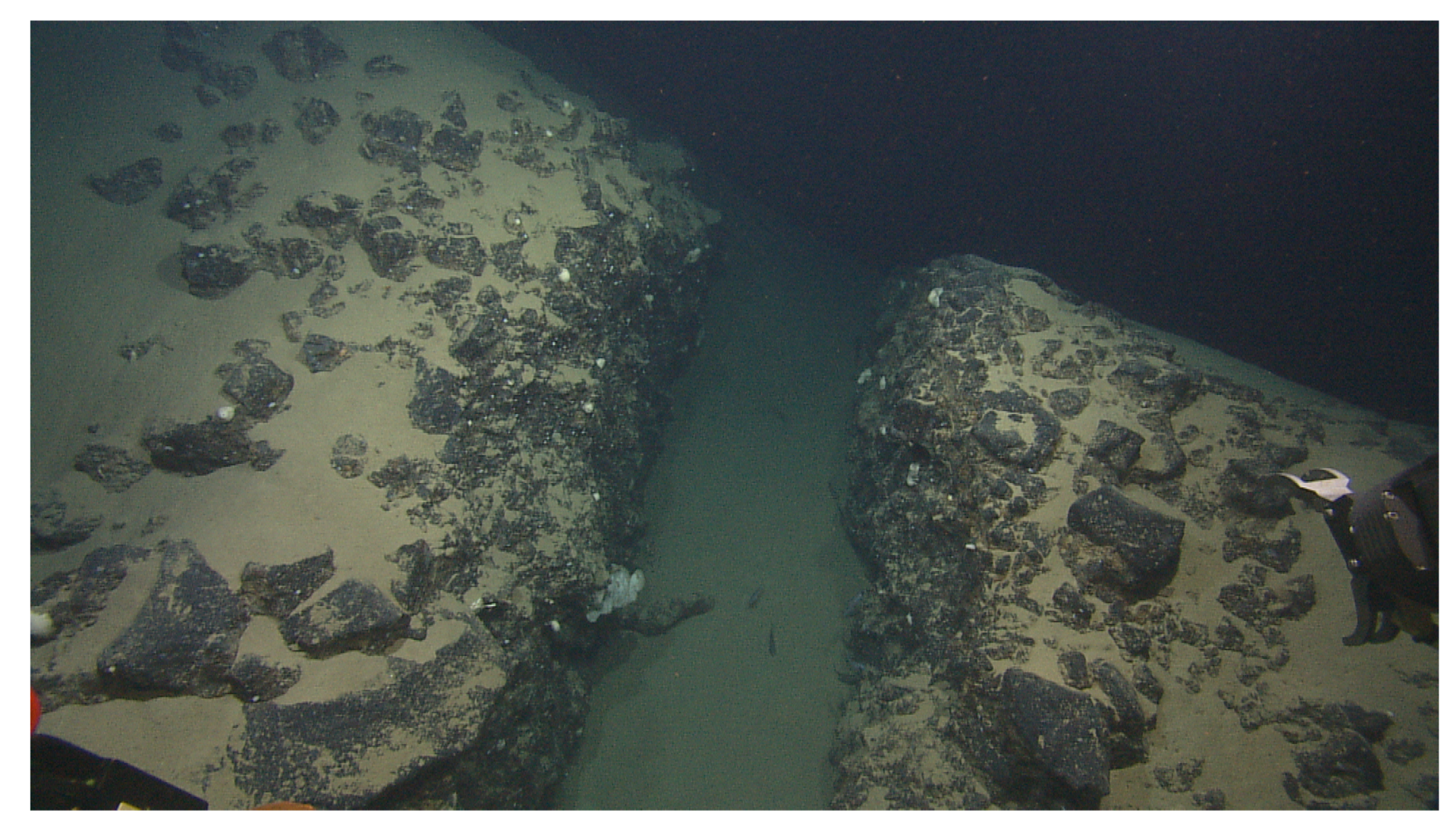
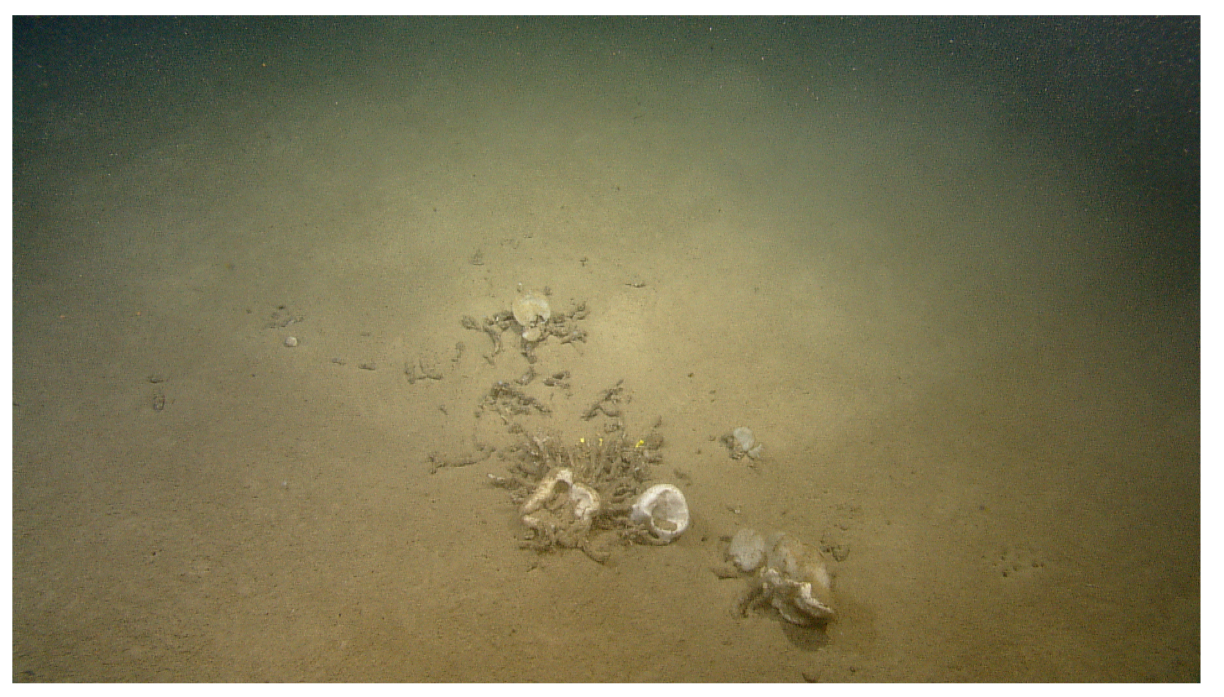
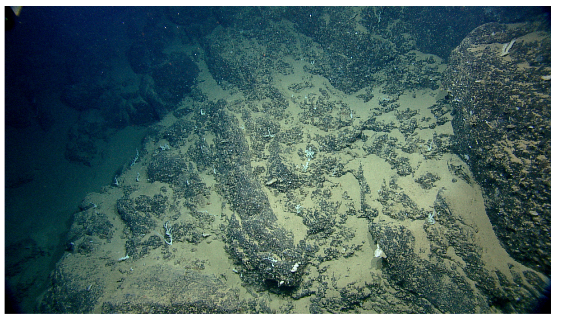
In the present work, vertical CTD profiles are presented for the first time with a full range of temperature and conductivity time series from the submarine caldera of Nisyros. The hydrothermal vent activity is relatively low and cannot be seen in the visual images captured by the cameras on board the ROV, as opposed to analogous findings from the Kolumbo submarine volcano that same year, where the activity was evident and the cameras captured ongoing plumes [15,17]. In 2010, Kolumbo underwent a period of unrest (Kolumbo2010), while in 2011, it was at rest (Kolumbo2011) [49]. These findings make it clear that hydrothermal venting occurs in different ways across periods of different activity. Understanding the data patterns as well as the underlying mechanisms stresses the importance of monitoring submarine volcanoes.
Comparing the data between the periods of rest and unrest within Kolumbo with our findings in Track 7 (Avyssos2010), we see that our results differ from both cases in Kolumbo. In Table 7, we compare the values of H and C from Avyssos2010 to the data published in Bakalis et al., 2017 (Kolumbo2010, Kolumbo2011). Note that all tracks presented in the table had a time-span of an hour and the missions in Kolumbo and Nisyros shared the exact same equipment and survey methodology; as such, they can be confidently used to distinguish different states of unrest in their hydrothermal vent fields. Kolumbo is considered to be one of the most dangerous submarine volcanoes in the Mediterranean [59]. Our results in Avyssos2010 differ from the results in Kolumbo in a way that makes it of lesser risk than Kolumbo2010, but also more prominently active than Kolumbo2011. During the resting period of Kolumbo, the values of temperature parameters are null, which is not the case in Avyssos.
On the other hand, the variance vs. lag time graph appears to have three regimes for conductivity in the data from both Kolumbo2010 and Kolumbo2011, while in Avyssos2010, we only have two regimes. Temperature in Kolumbo2010 has three regimes as well, while in Kolumbo2011, temperature variance is parallel to the time axis, which results in a γ exponent equivalent to zero. In Avyssos2010, no parameters are null. The morphological structure of the two volcanoes are different, which might result in the difference in behavior after a time period, thus creating three regimes for Kolumbo and two regimes for Avyssos. The two submarine volcanoes differ in shape and size as Kolumbo has a circular cone with abrupt steep slopes, while Avyssos is a 3 km wide volcano [6].These geomorphological characteristics make Kolumbo a closed thermodynamic system, and Nisyros an open one. However, the thermodynamic state cannot account for the null values of temperature parameters during the resting period of Kolumbo, considering the homogeneity of hydrothermal fluid outflow.
The statistical moments in Kolumbo2010 appear to have two distinct regimes in the moments vs. lag time graph, with a turning point at Δ = 5 s. In Kolumbo2011 however, the turning point is at Δ = 1 s, the same as in Avyssos2010. This can be interpreted as an indicator for similar dynamics to Kolumbo2011 despite some structural differences in the variance function.
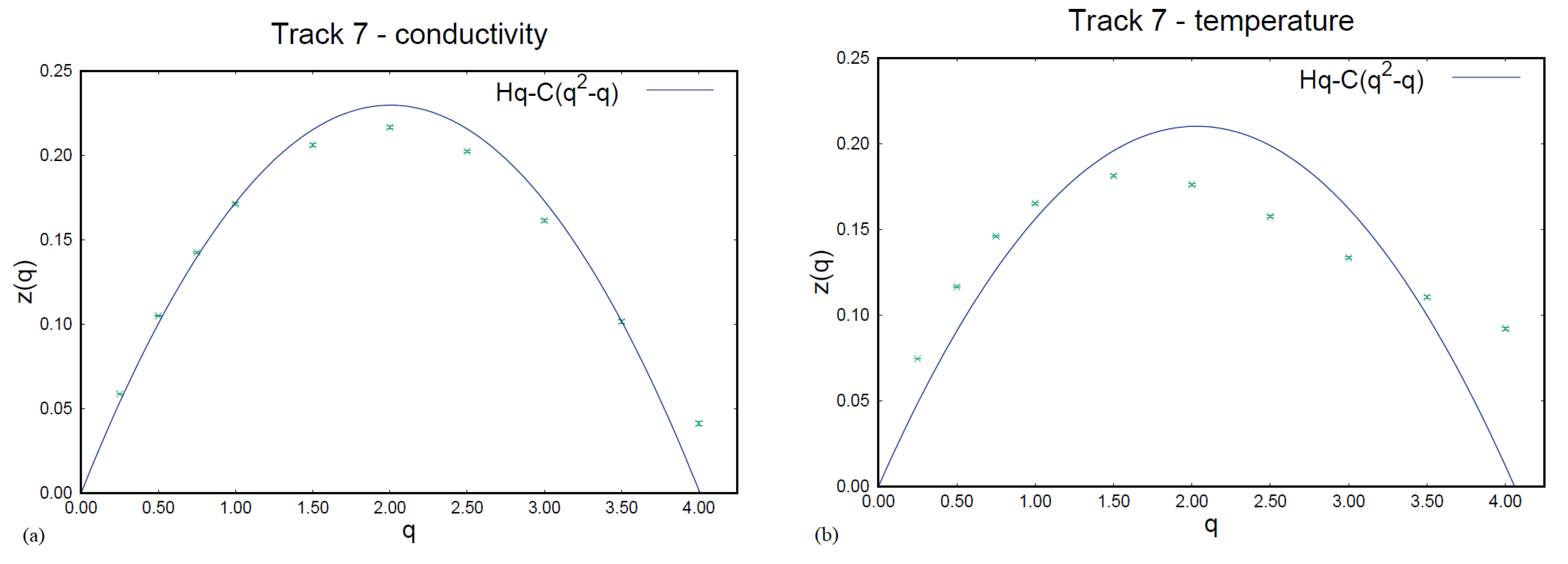
Last, the structure function has a convex shape in Kolumbo2010 and in Avyssos2010. As for Kolumbo 2011, the structure function of conductivity appears to have a similar behavior, whereas for temperature, z ( q ) is 0 for all values of q.
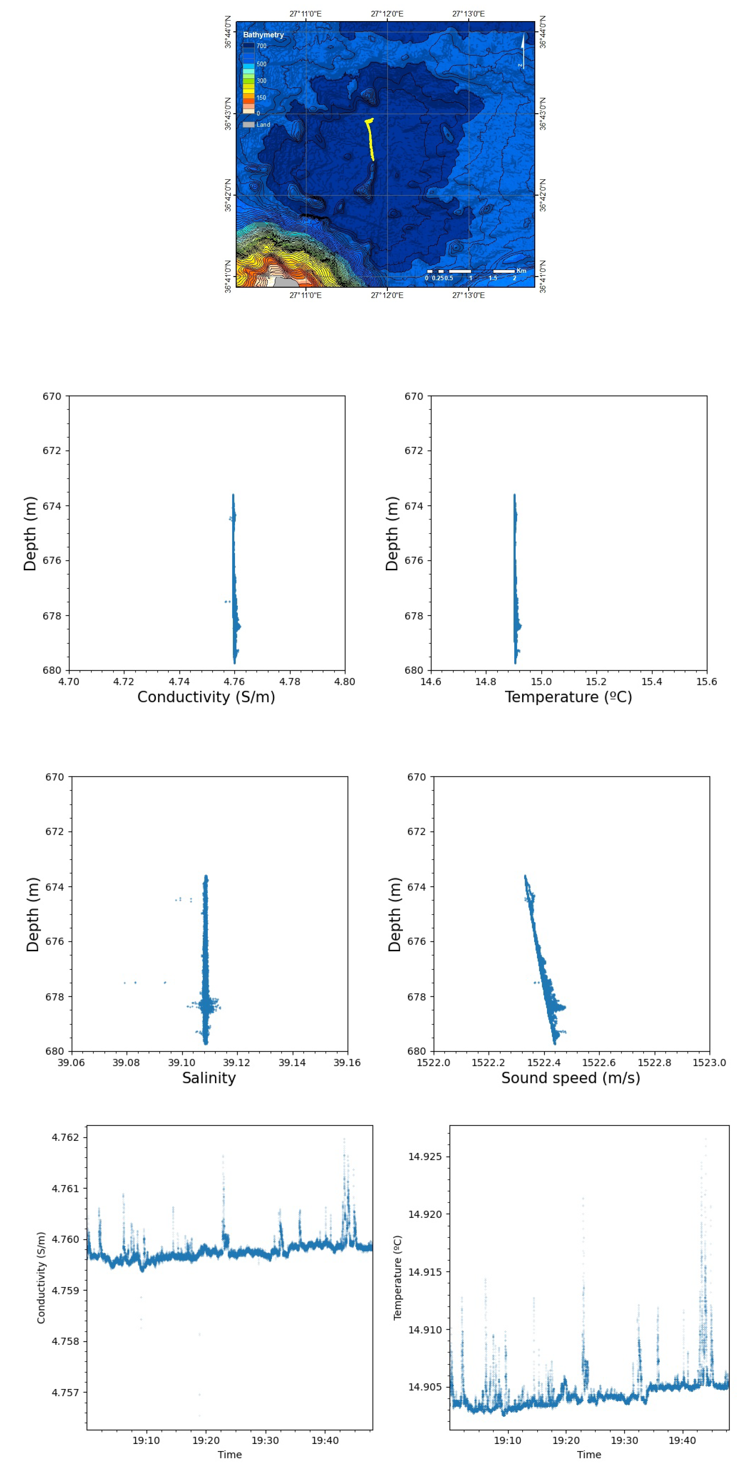
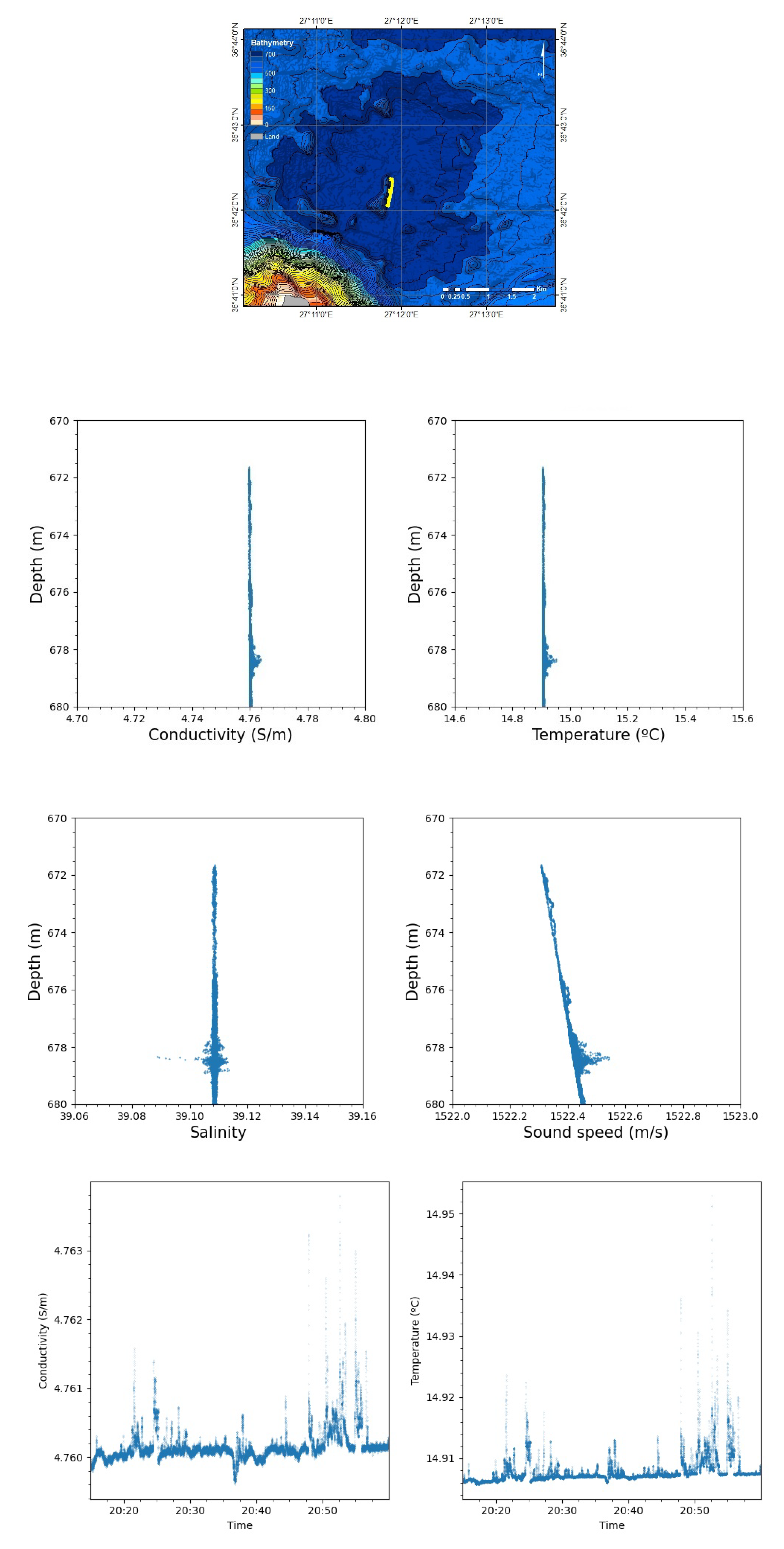
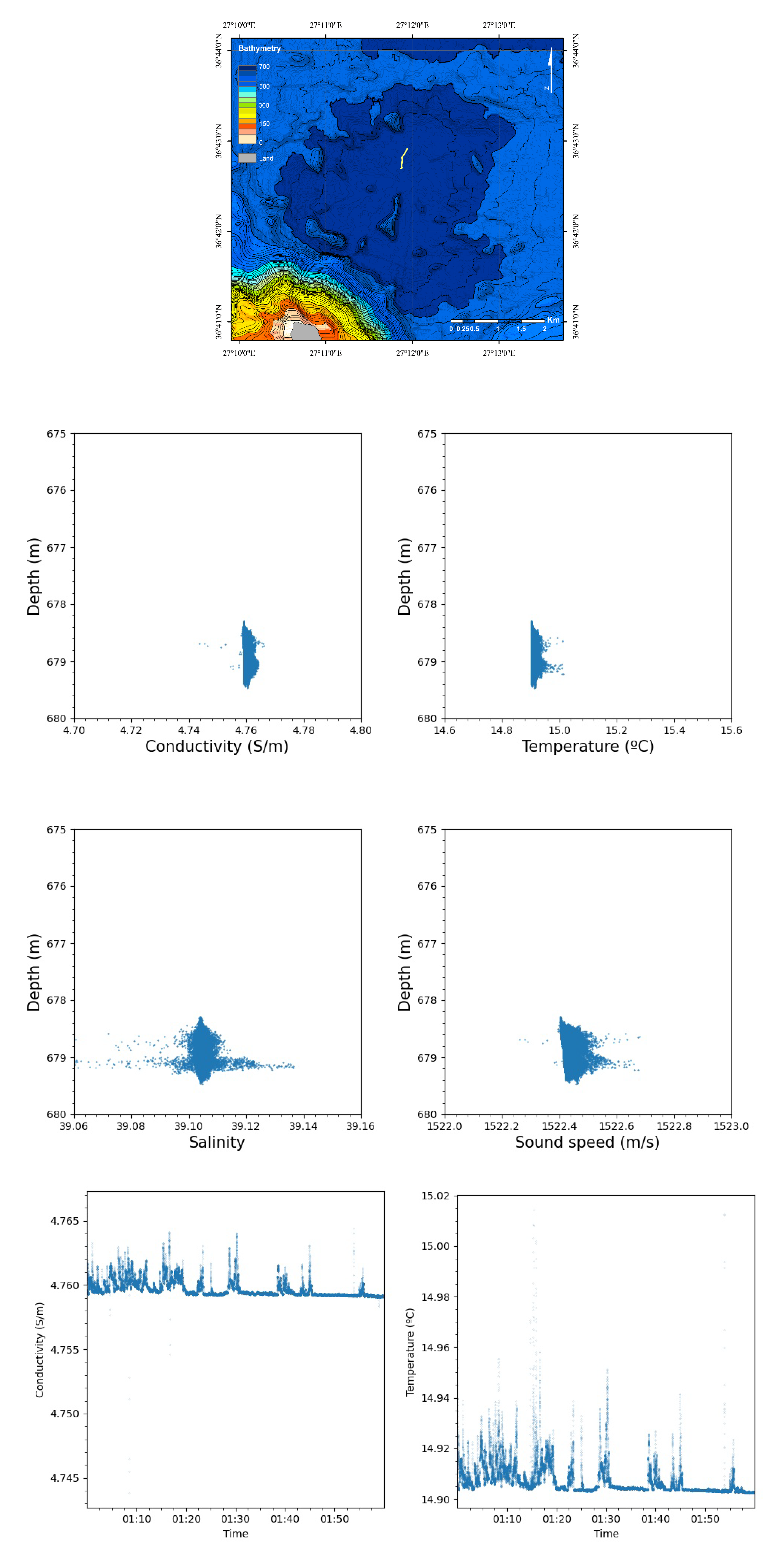
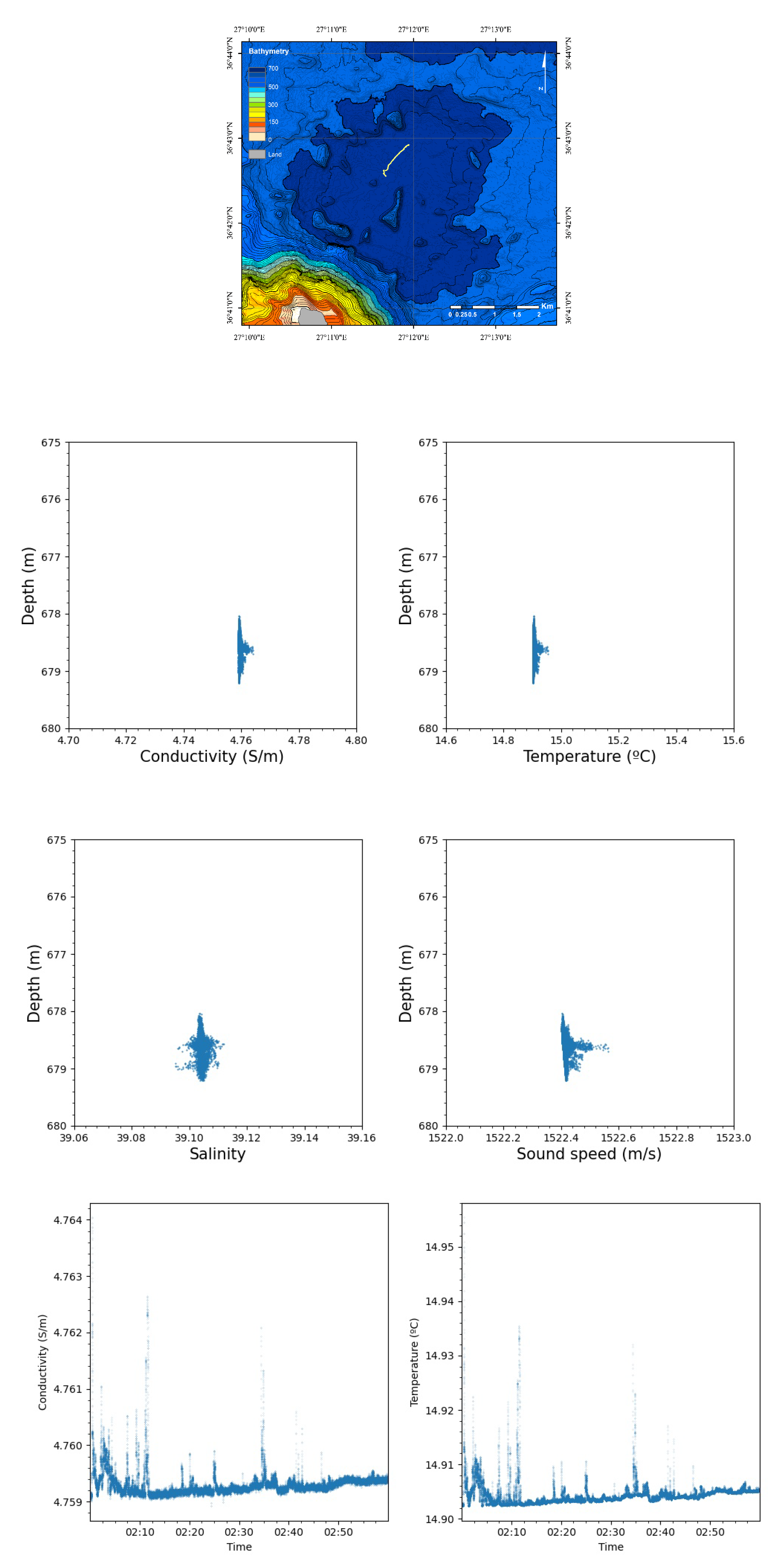
Regarding the time series in Avyssos, the first results from the survey [47] originate from a simple data set gathered in 10 October 2010, during a total recording time interval of 1 h and 30 min. That time series preceded the data in the present work and were recorded over a specific location while the ROV was slowly hovering. According to those results, when the volcano is at rest, conductivity seems to obey a stationary process, and the crater of the volcano is in direct contact with the overlying water environment, thus defining an open system. In this research, the same methodology was used to extend the analysis of the entire data set gathered from the deepest parts of the caldera (10 and 11 October), covering approximately the full area under investigation.
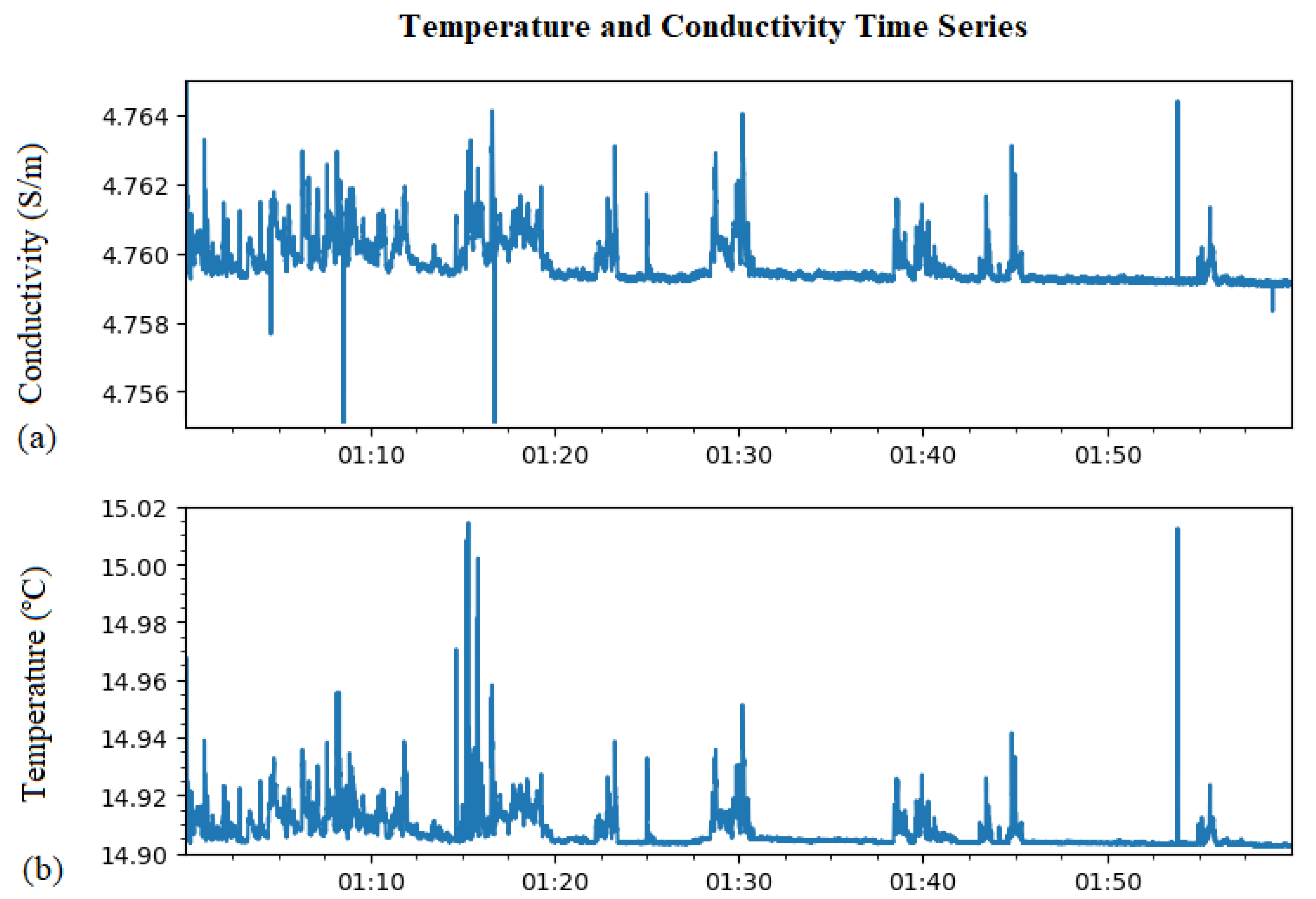
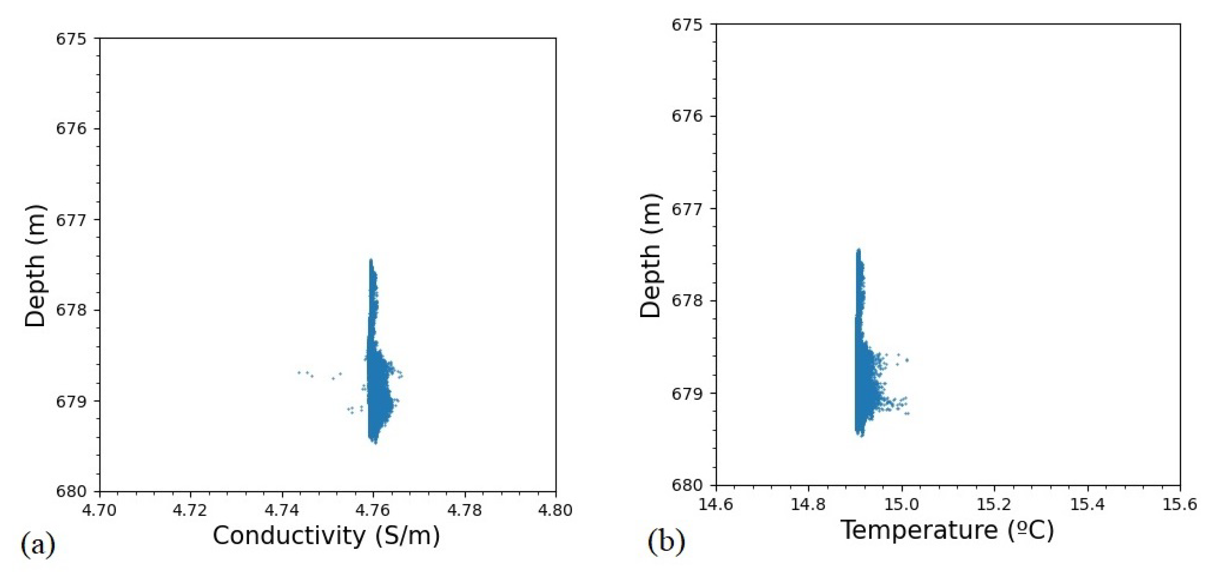
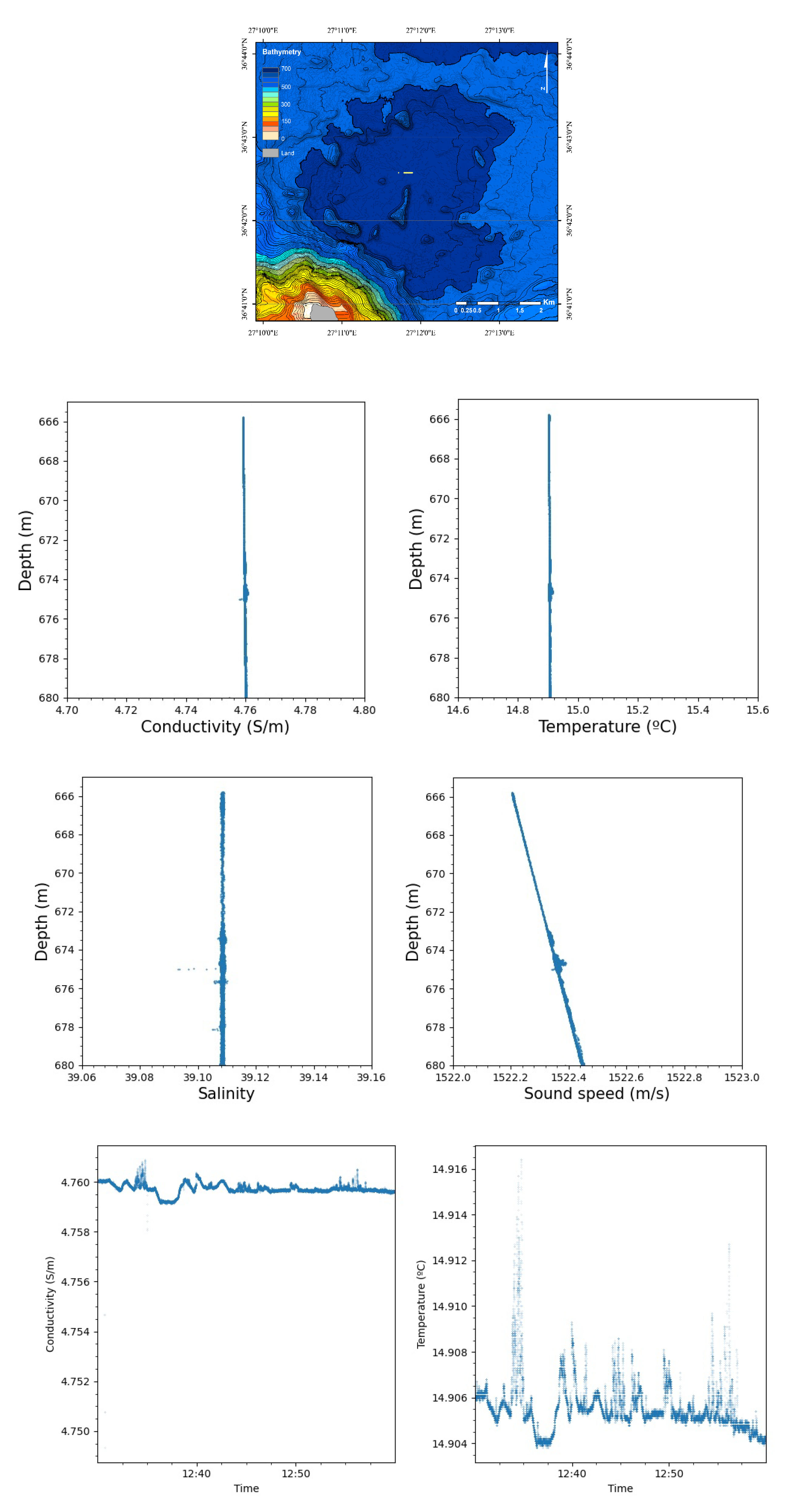
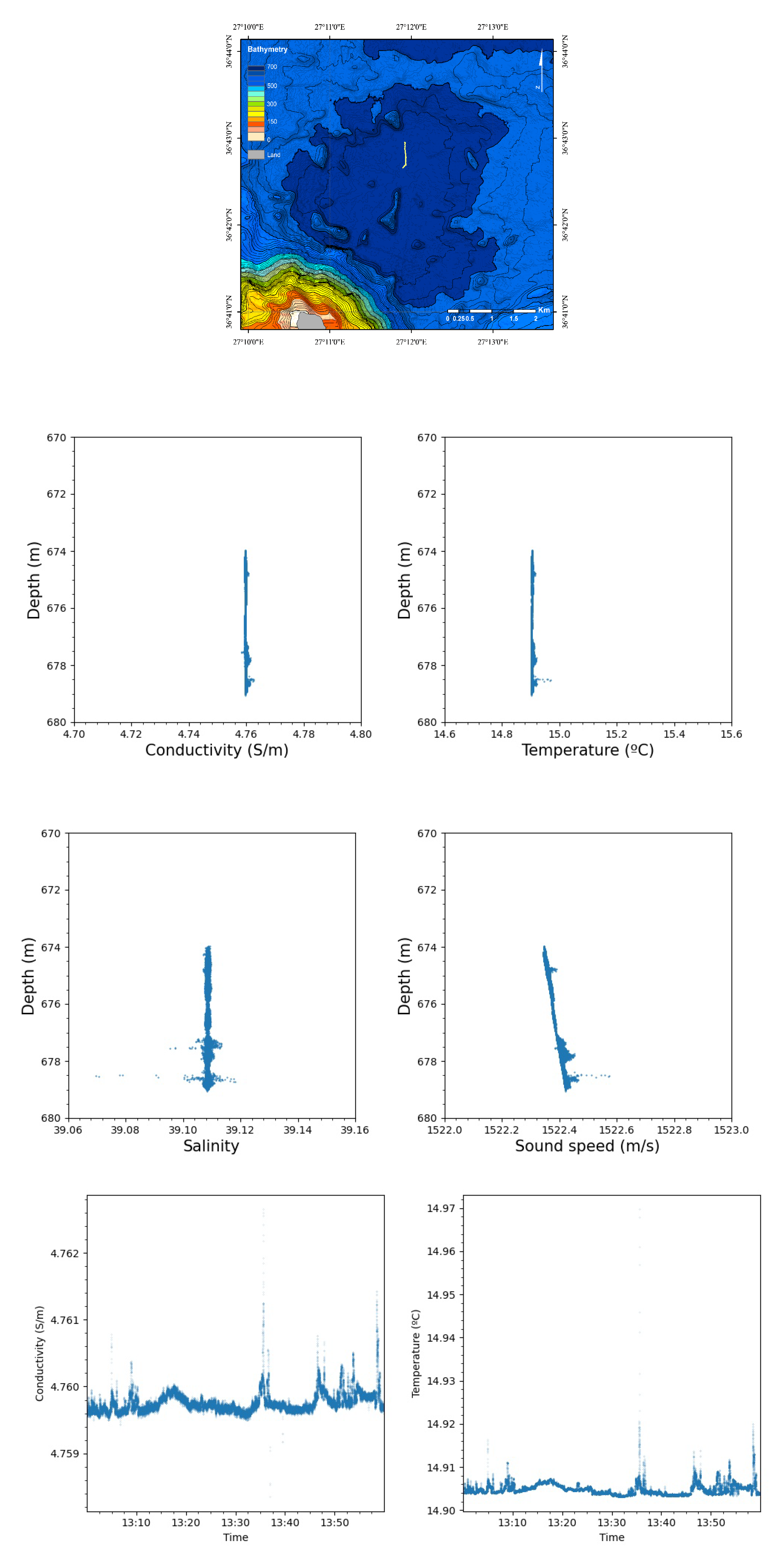
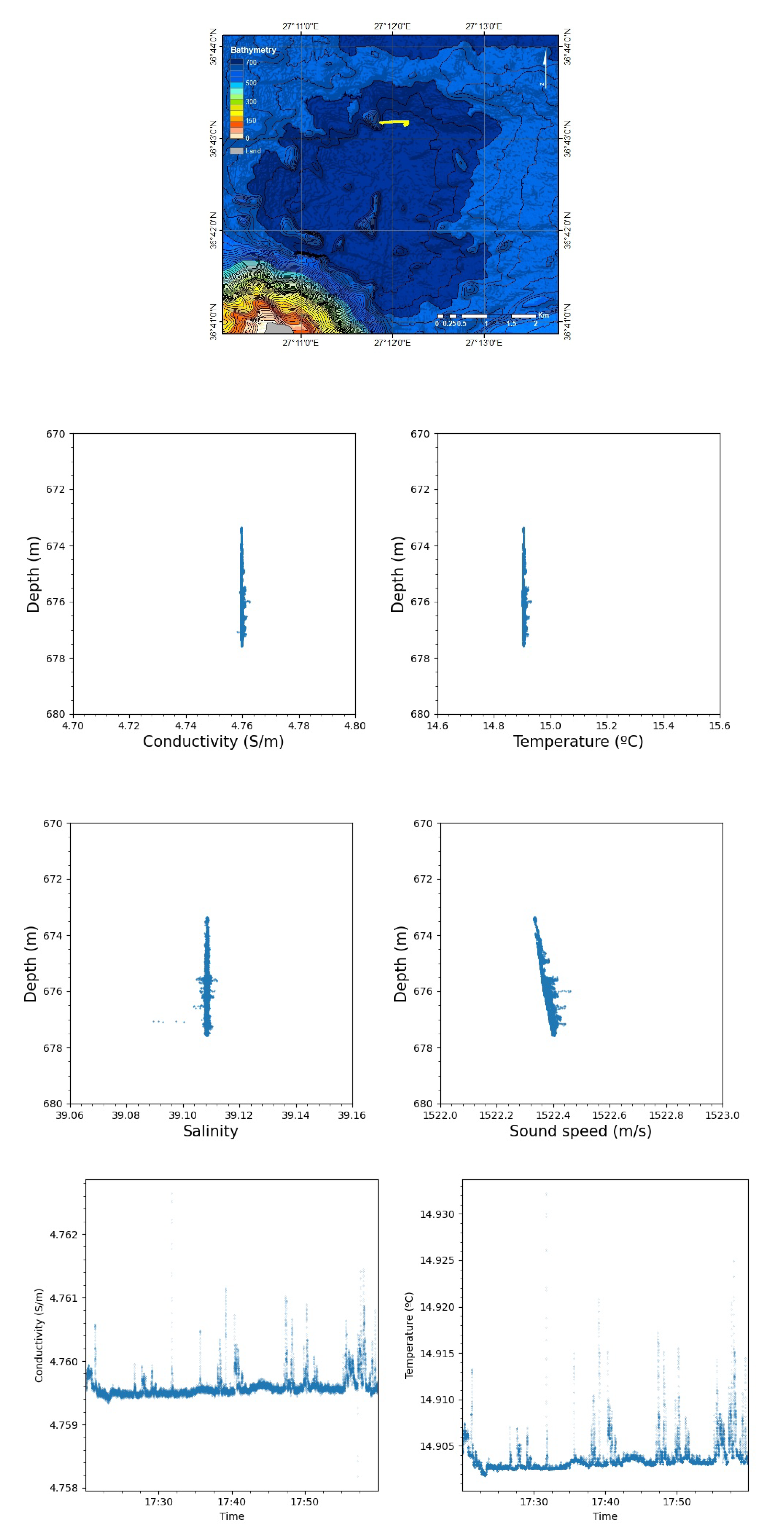
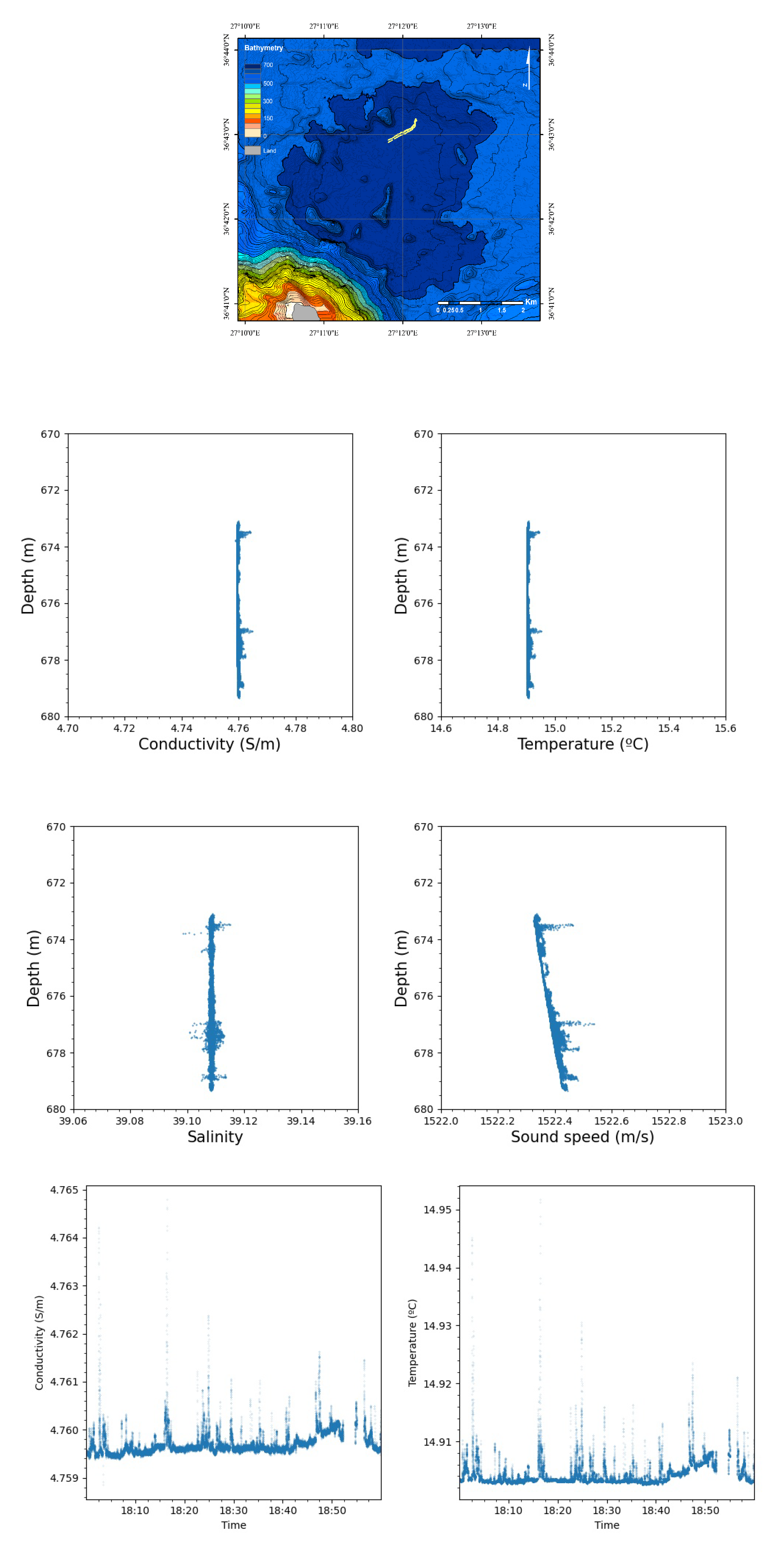
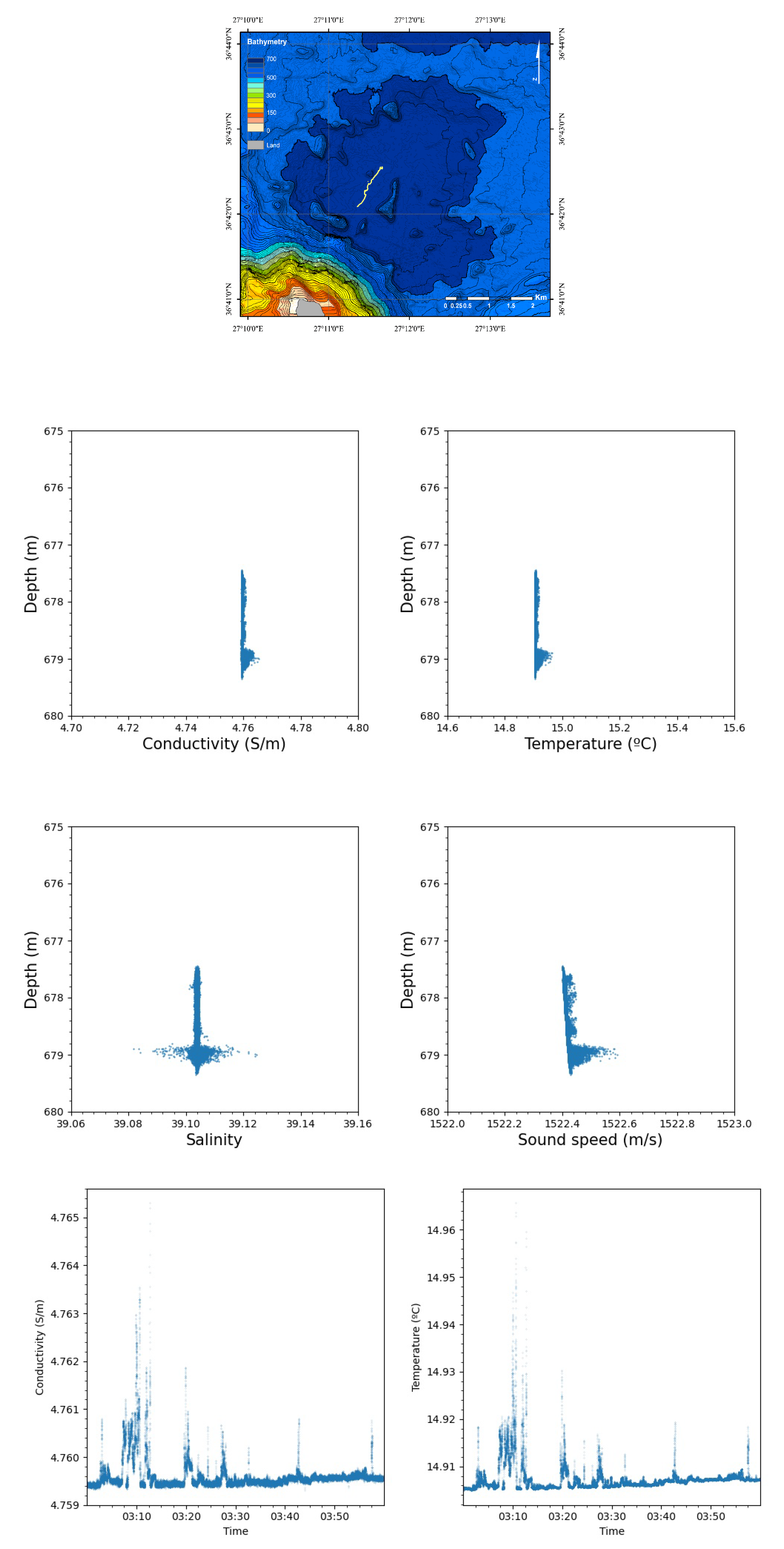
We consider anomalies in the time series to be spikes that deviate from the baseline. The baseline in the case of Track 7 (Figure 13) would be a line almost parallel to the time axis at about 4.756 S/m for conductivity and at approximately 14.91 C for temperature. Both parameters would be otherwise stationary and would evolve in time in a manner that would prove irrelevant to a baseline, where there no activity (as is the case for Kolumbo2011). We use these values as a reference to evaluate the anomalies. For conductivity, the most prominent spike diverges at 0.9 % from the reference baseline, while for temperature, the respective percentage is 10.5 % . The above observations are similar for all tracks presented in here (such as Track No 4, etc.). In Kolumbo2010, conductivity spikes scale at a maximum of 130 % (spike = 5.5 mS/m, baseline = 4.2 mS/m), while temperature anomalies spike at 480 % (spike = 21 C, baseline = 16.2 C), which shows the near-explosive state of the volcano. The case of Avyssos2010 clearly differs to the case of Kolumbo2010. Conductivity and temperature parameters in Avyssos2010 spike at a much smaller scale in terms of absolute values, as well as percentage, compared to Kolumbo2010. In Kolumbo2011, spikes appear to be random and constant with no particular baseline to reference any anomalies (see Figure 1c,d in [49]).
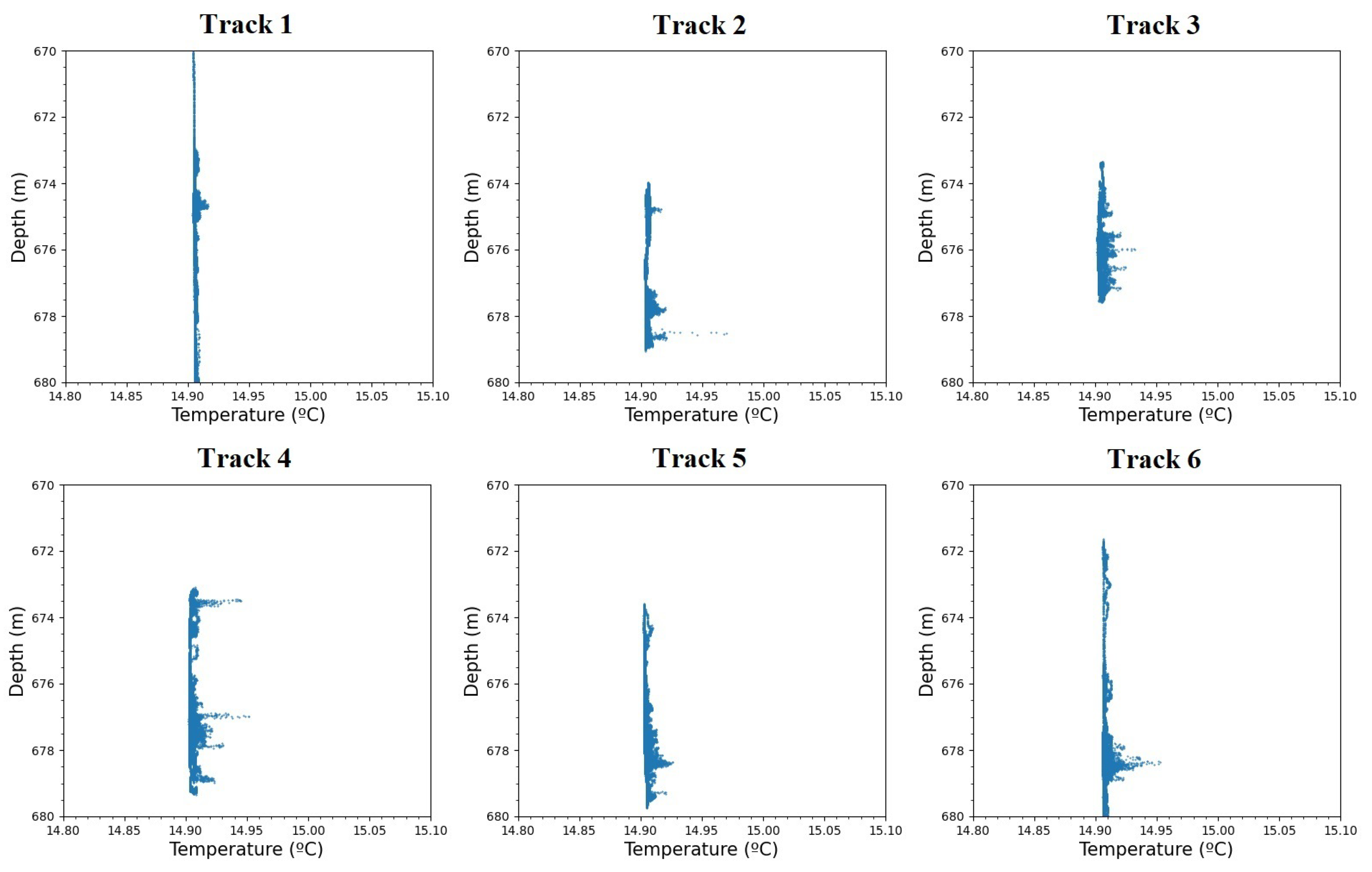
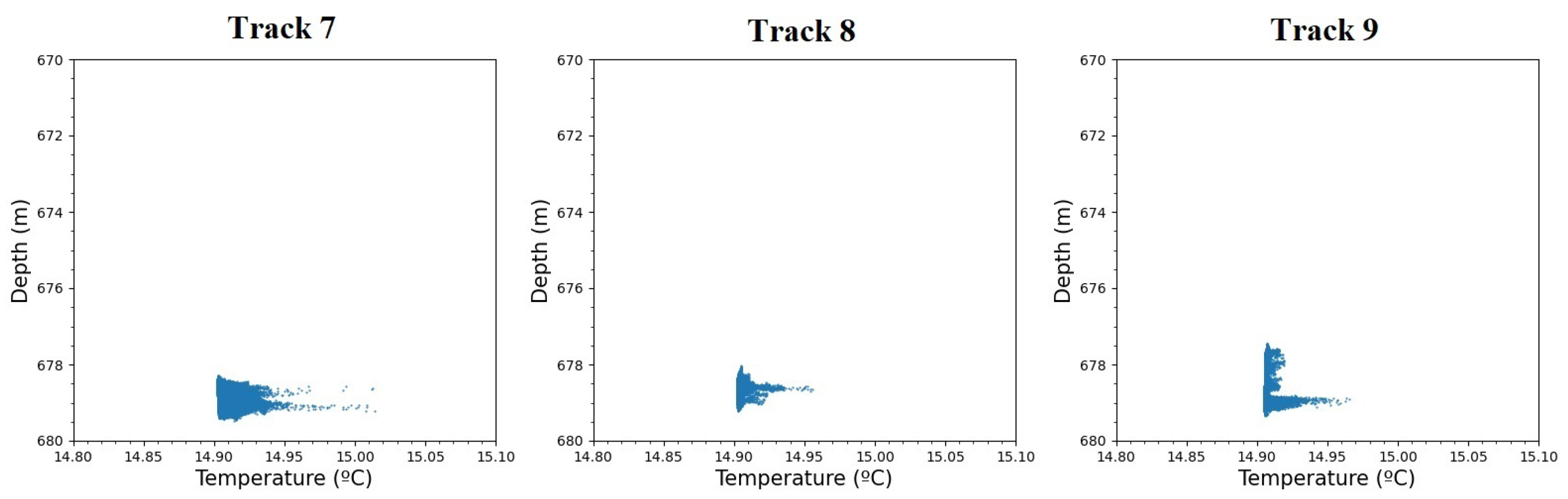
Activity is evident in both time series and vertical profiles, and seems to be consistent among conductivity and temperature, which are the main points of focus. The time scale peaks appear at the exact same point in time (
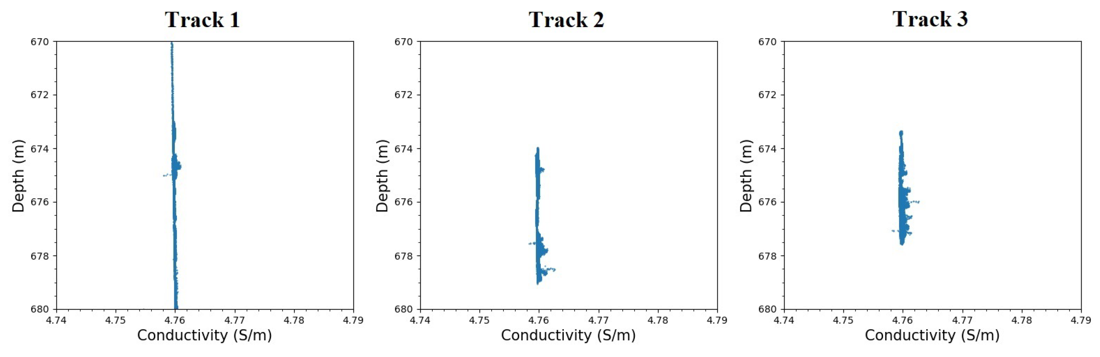
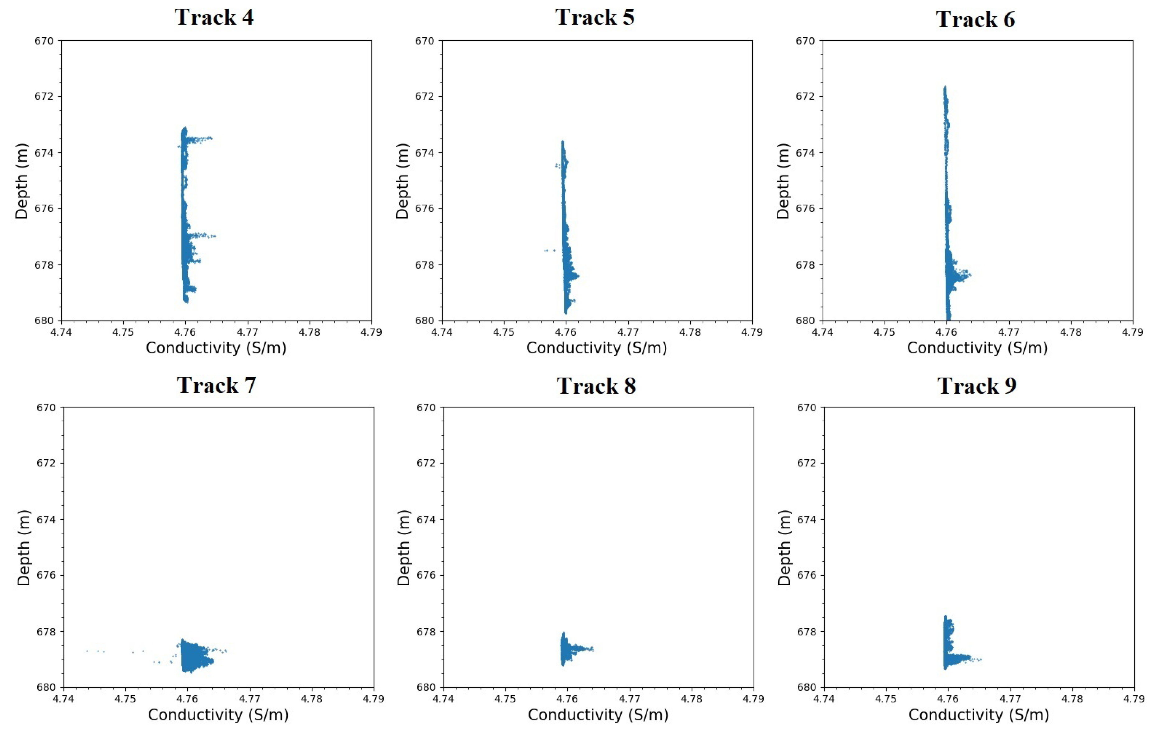
Figure 13), whereas the vertical profiles appear at a similar depth for both the parameters (Figure 9 and Figure 10). In the case of the vertical profiles in Track 7, we notice spikes that skew at 1.6 % for conductivity and 11.7 % for temperature, respectively.
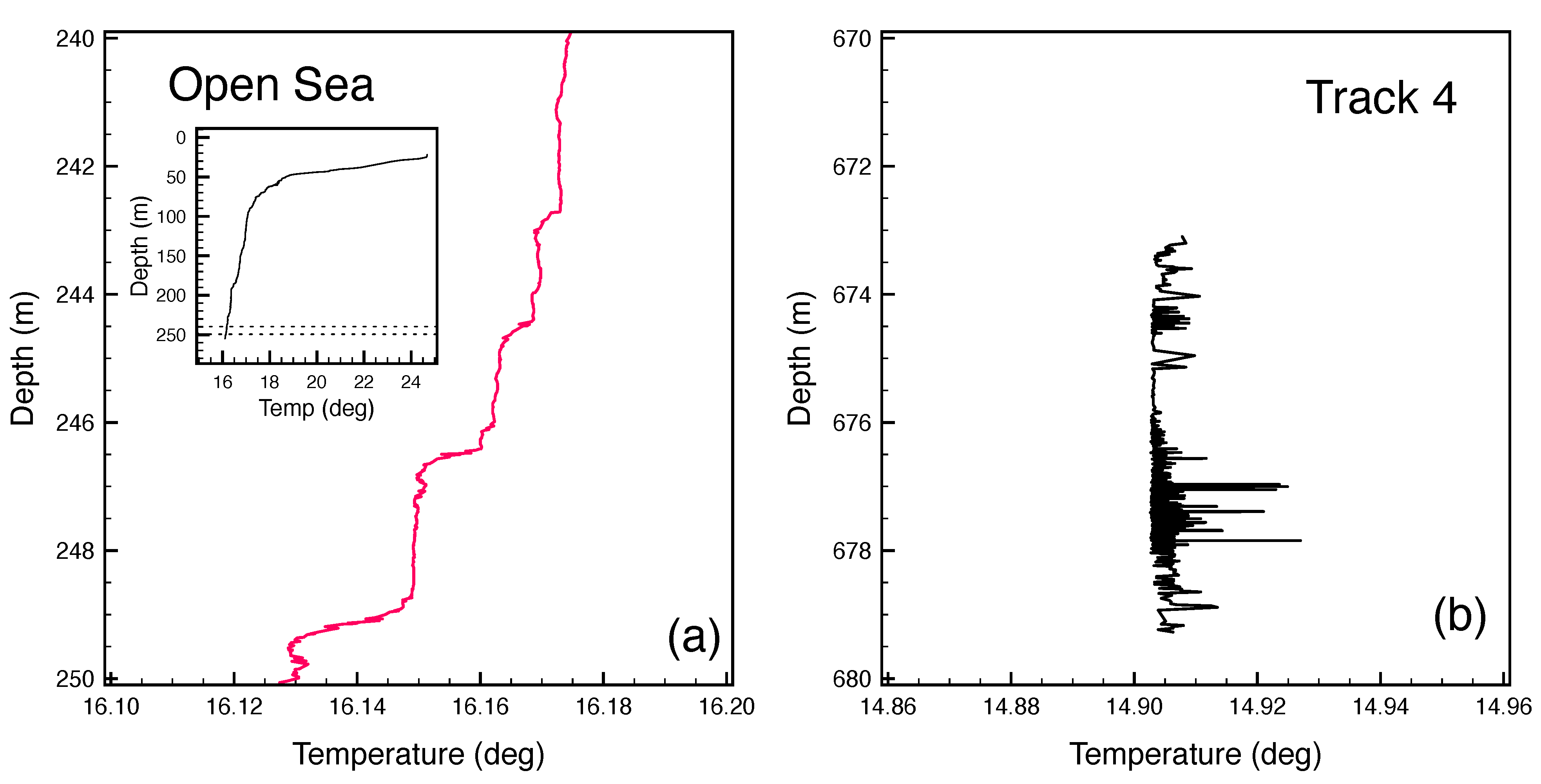
An additional piece of evidence is the comparison of the present vertical CTD profiles with reference CTD data. As such, a vertical profile between 20 and 250 m recorded with the exact same methodology and instruments during the same mission (but earlier time) in an open sea location, where no hydrothermal activity exists, has been considered and is shown in Figure 21a. The inset shows the full CTD profile, while the main panel shows a magnified region with the same x- and y-axis ranges as with Figure 21b which shows Track No 4 for comparison (see also the caption of the figure for further comments). From this comparison, it becomes evident that the vertical CTD profiles in Avyssos differ completely from respective (“reference”) CTD profiles in open sea, where effects such as mixing, thermal layers, turbulence, etc. can affect their shape. In this case, no abrupt changes are observed, rather step-like changes occur at certain depths. The situation can be easily generalized by comparing the open-sea vertical profile with any one shown in Figure 10.
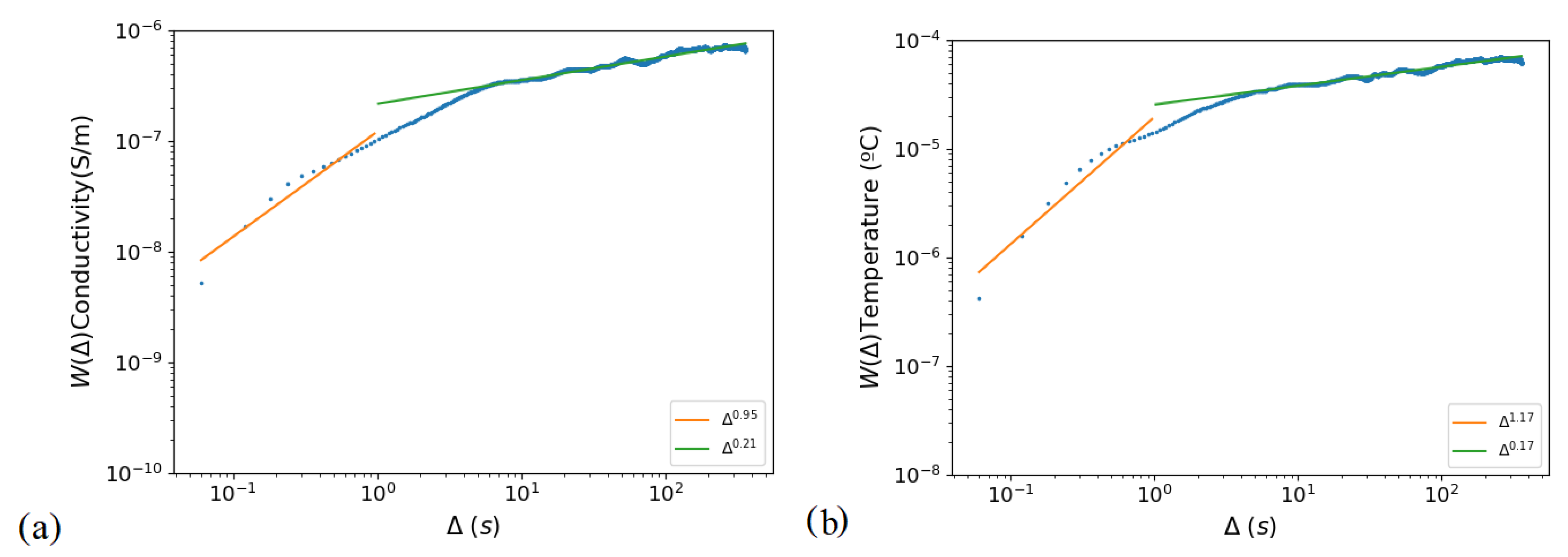
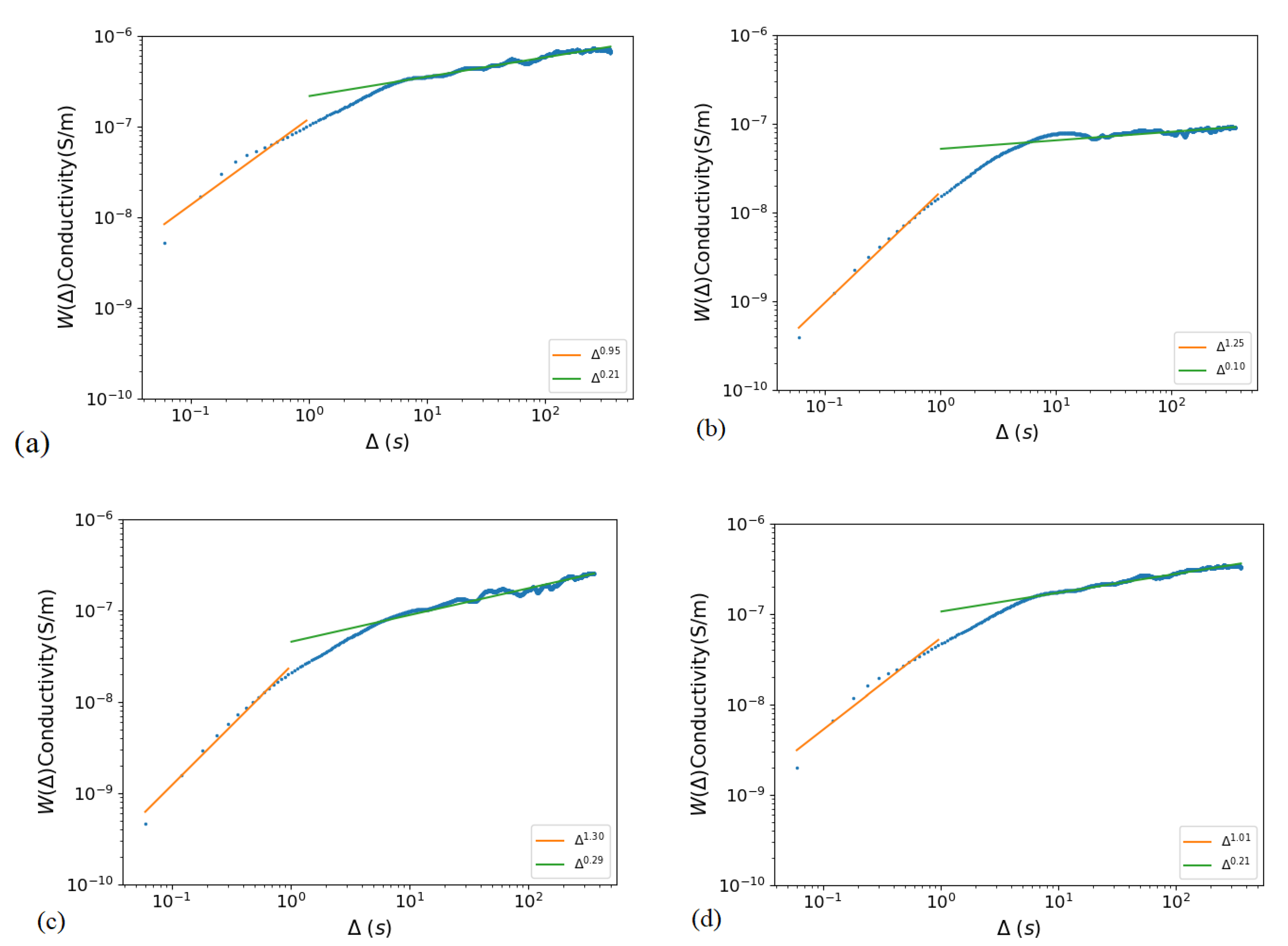
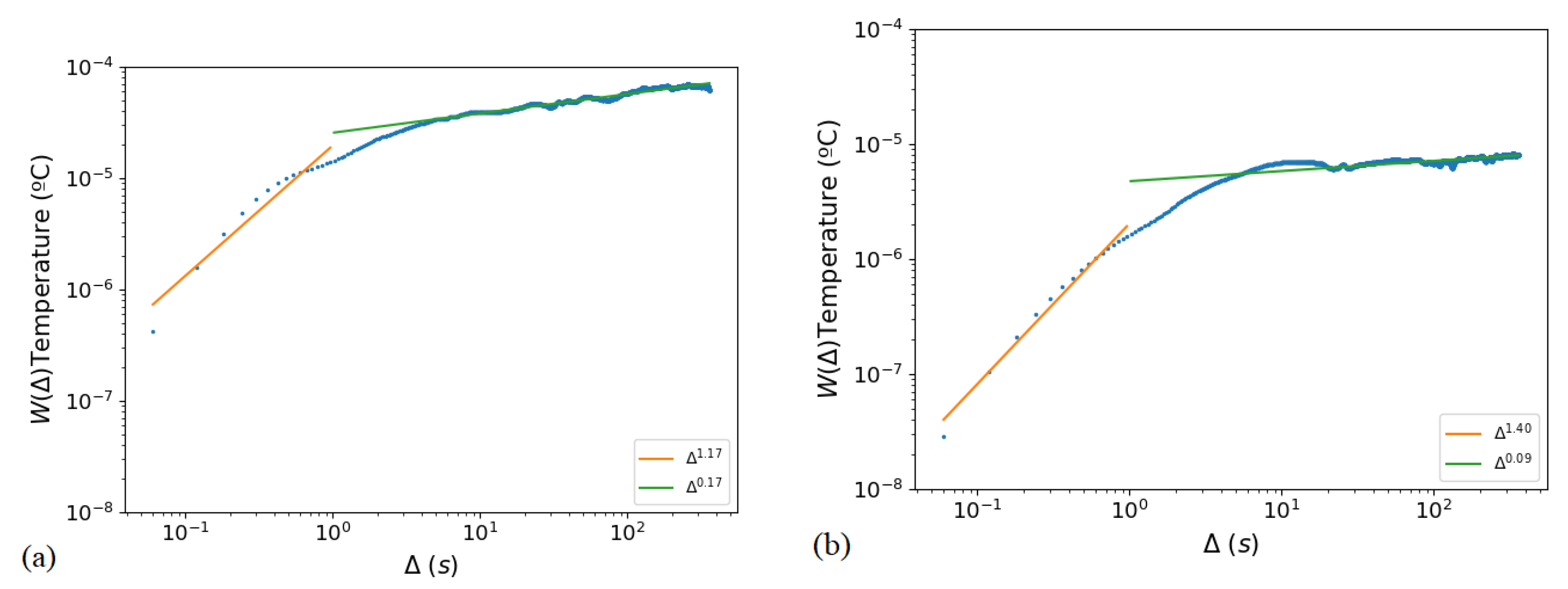
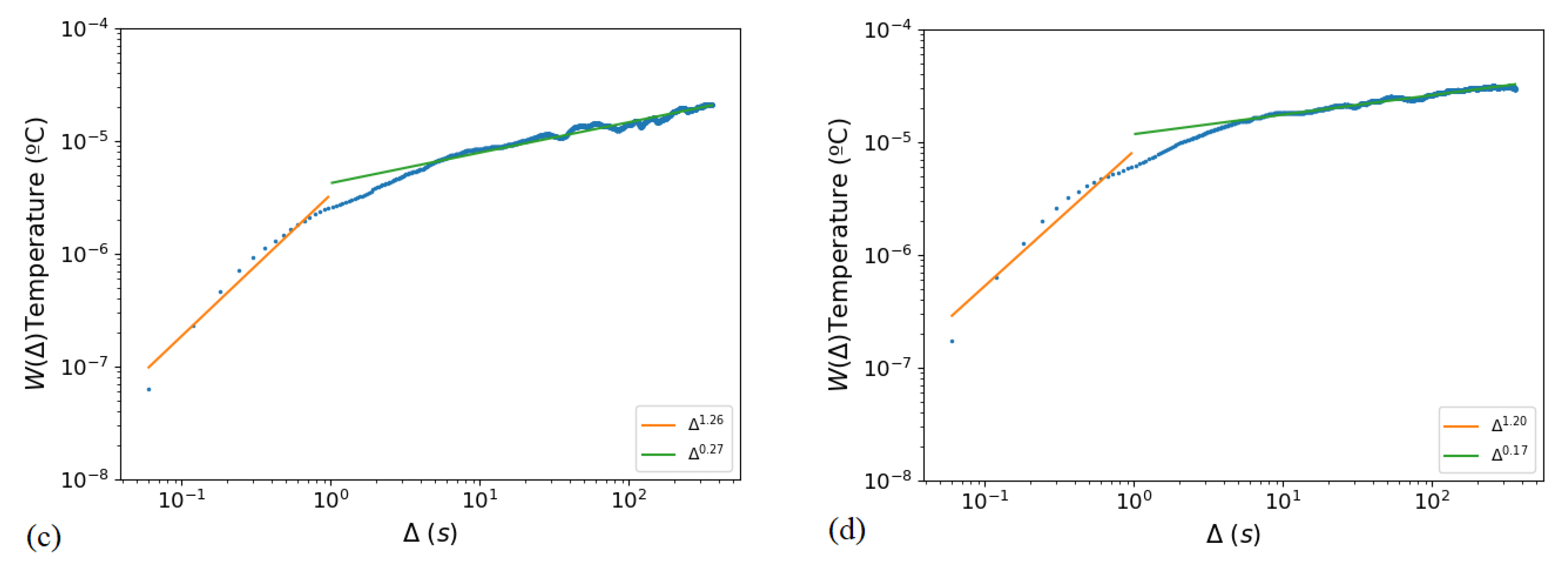
Despite the activity of the volcanic field in Avyssos being weak and almost homogeneous in its entirety, as shown in the overall ROV surveys, the values of the exponents γ are scattered for both conductivity and temperature in the first regime (Table 2 and Table 3). On the one hand, conductivity shows a normal to a slightly super-normal behavior, with the only exception in Track 1, where points are either uncorrelated or display persistent trends during reduced time intervals. On the other hand, the scaling of all tracks for the temperature indicates persistence. In the second regime, both fields present a strong anti-persistent motion, which mirrors on their slow changes.
These values reflect the existence of an active vent field, the behavior of which is not persistent. In addition, the value of the Hurst exponent indicates some delay between two similar value pairs in a time series. This situation reveals the existence of weak, homogeneous sources of hydrothermal fluid outflows, which are found throughout the entire examined area.
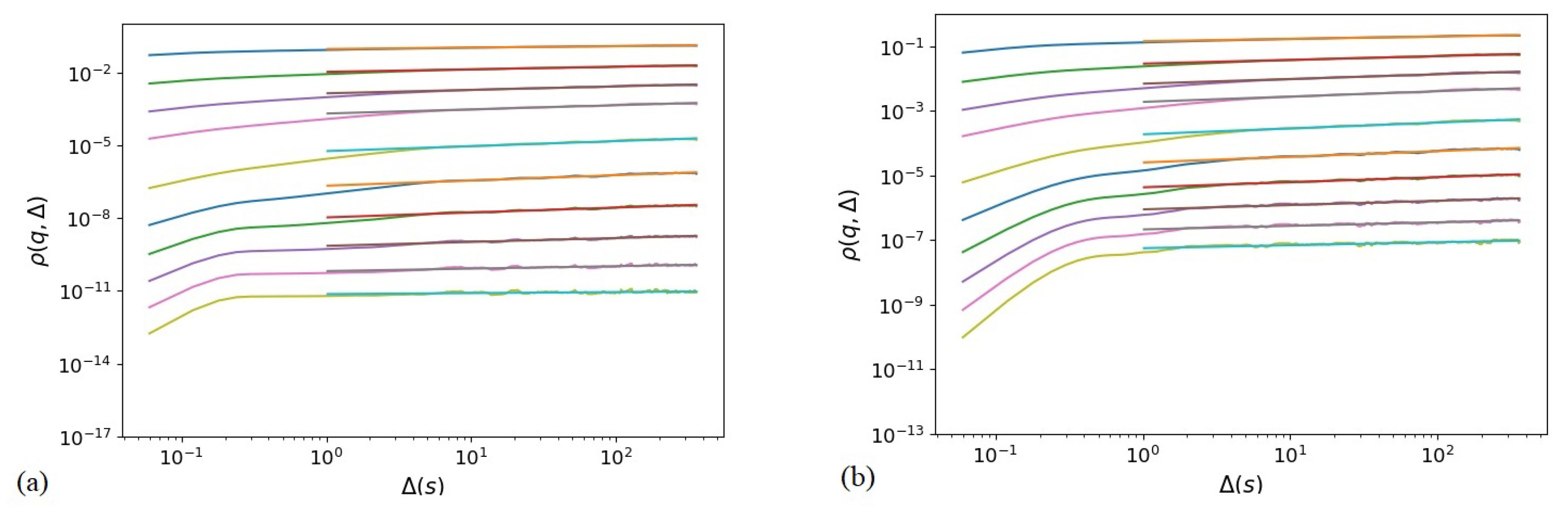
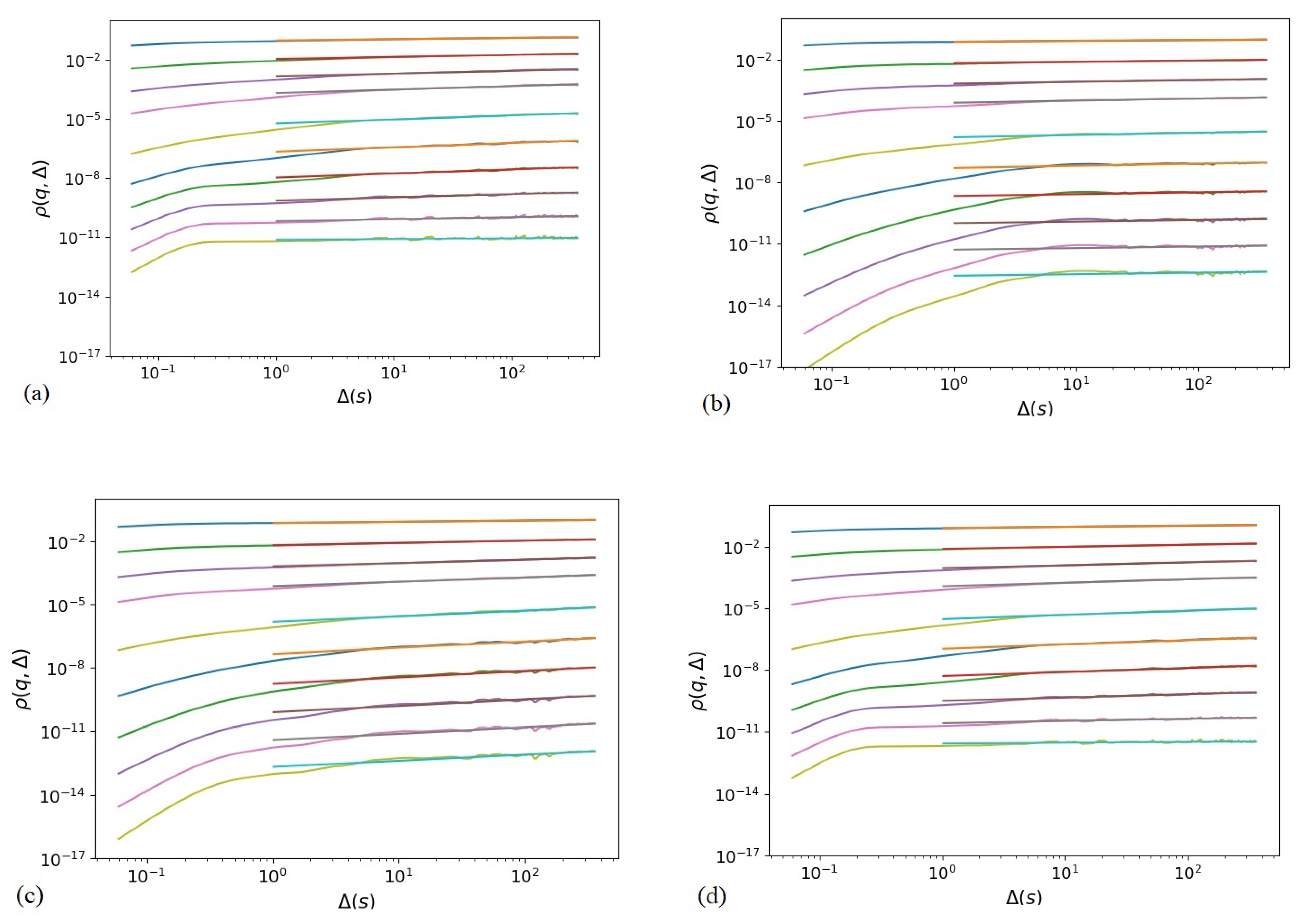
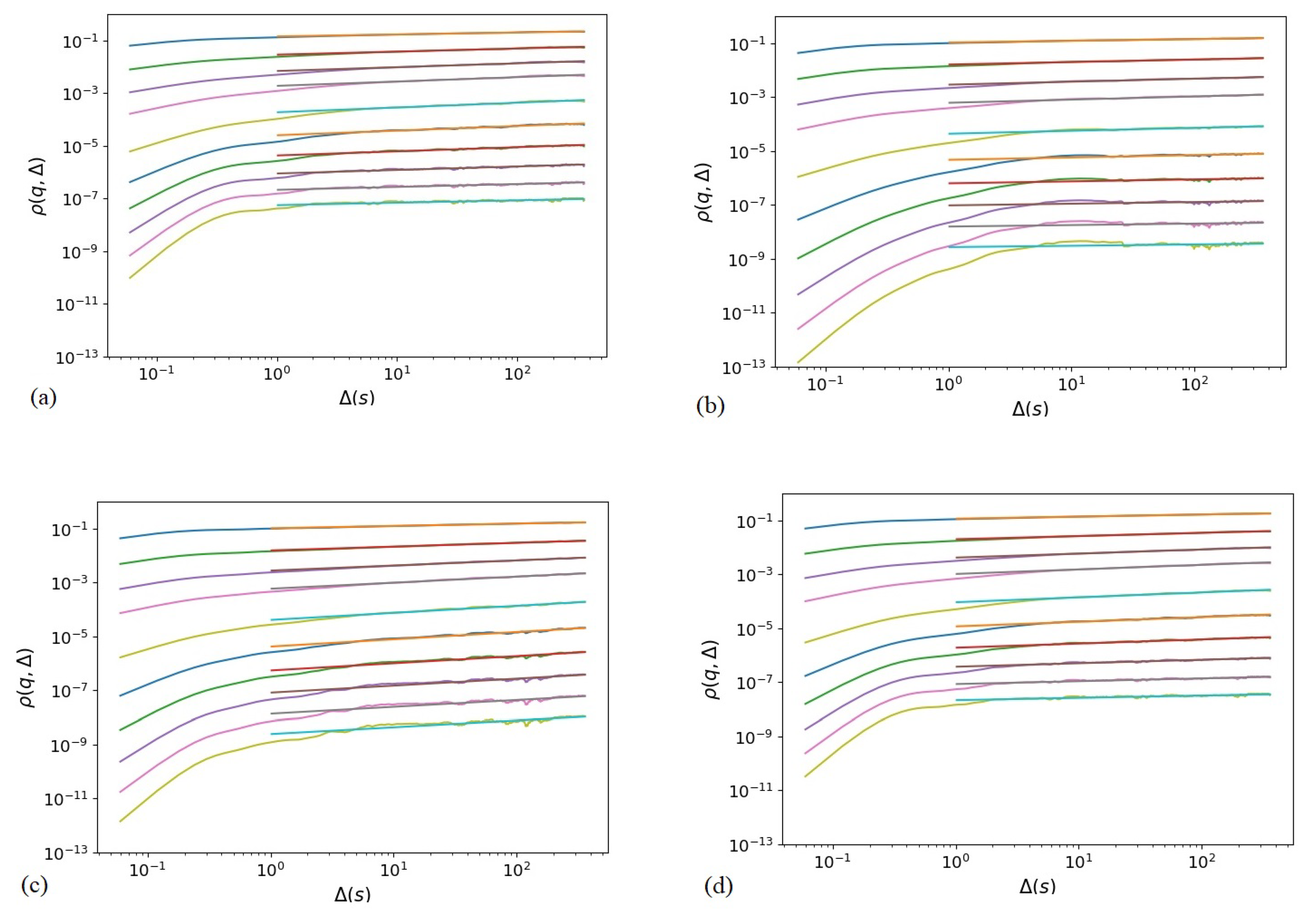
The exponents of Δ appear to have similar behaviors across various locations inside the caldera, as well as among conductivity and temperature. The similarity in behavior across parameters is also verified in their time series and their profiles. In Appendix A, the full list of maps, CTD profiles, and CTD time series for all Tracks mentioned in Table 1 are presented for Avyssos.
The analysis of the recorded time series of temperature and conductivity just above the Avyssos submarine volcano shows that both parameters seem to present an initial multiplicative behavior reflecting the mixing of at least two different random processes, which then turn to be quasi-stationary.
In the case of non-persistent hydrothermal activity, we expect to find dissimilar results when analyzing data from a longer period of time while the ROV remained at the deepest locations possible. As the analysis was performed while the ROV was hovering and slowly moving over a wider area at the same time, a direct comparison with the previous work in Nisyros [47] cannot be made. This seems to be distinctly reflected on the behavior of the conductivity time series, which have been found to be completely different from the single time series reported in [47]. The conductivity time series reported here present similarities with the temperature time series, which is not the case in the earlier work reporting results over a specific location in the vent field.
Comparing the results of the hourly intervals to the total of three hours (Tracks 7, 8, and 9), we find differences in the behavior of the moments ρ ( q , Δ ) . These differences are possibly attributed to a number of factors. One factor may be the particular geomorphological features of the caldera along these tracks, as the caldera bottom is not smooth. In addition to that, the ROV hovered over the seafloor in a slow motion, instead of being absolutely still. Finally, the weak variations in the underlying hydrothermal activity across the caldera can also potentially lead to these differences.
Although generally considered inactive, the island of Nisyros exhibits the basic properties of active volcanic regions in quiescent periods [40]. From time to time, a period that may range from months to years [40], Nisyros enters a period of unrest which leads to seismic activity, significant temperature increase in the hydrothermal system, gas detonations, steam blasts, mudflows and ground deformation [42,43,60,61,62,63,64,65]. The possibility of Nisyros entering the next periodic unrest in a few years cannot be fully excluded as suggested by the existence of weak hydrothermal sources found within the caldera.
Moreover, the present work confirms that the application of the GMM in geosciences seems to find a clear-cut way, at least in terms of analyzing CTD time series, to investigate the underlying mechanisms governing the activity of hydrothermal vent fields in submarine volcanic areas. As the GMM has been used in econometrics, commercial packages offering GMM analysis tools in geosciences are still not widely available, to the best of our knowledge. Based on our experience working with GMM to analyze CTD time series, we argue that such computer codes could significantly reduce the time needed to reach conclusions, something particularly useful for cases where the risk of natural hazards should be assessed and mitigated promptly. It is clear that monitoring natural hazards associated to submarine hydrothermal vent fields with state-of-the-art instrumentation is the spear to mitigate those risks. However, the continuous increase of computing power facilitates the introduction of advanced tools, such as Artificial Intelligence and Machine Learning, and can offer the chance to statistical methods, such as the GMM, to play an enhanced role as a complementary approach. An additional advantage seen in the present research is that the combination of a mathematical model (GMM) with fast, state-of-the-art sensors (ROV-based CTD) that collect data can provide a framework for understanding dynamic processes in the marine environment that could completely remain unknown by using traditional techniques of exploration (such as visual inspection or use of samplers).

Author Contributions

conceptualization, A.D., T.J.M., P.N., and A.G.; methodology: E.B. and F.Z.; software: A.D. and M.M.G.M.; geological data and mapping: A.D., P.N., and A.G.; data analysis: A.D., M.M.G.M., and T.J.M.; resources: P.N. and A.G.; manuscript authoring: all authors. All authors have read and agreed to the published version of the manuscript

Funding

This project has received funding from the Hellenic Foundation for Research and Innovation (HFRI) and the General Secretariat for Research and Technology (GSRT), under grant agreement No 1317. Swath mapping was a part of the GEOWARN project (Contract no: IST-1999-12310). TJM and PN acknowledge partial support by RAMONES, funded by the European Union’s Horizon 2020 research and innovation programme, under grant agreement No 101017808.

Acknowledgments

We thank Ioannis Madesis for useful discussions. MMGM acknowledges partial financial support by the ERASMUS+ mobility program. ROV surveys were supported by the Institute for Exploration (IFE-USA) and the collaborative project “New Frontiers in the Ocean Exploration”. The officers and the crew of the E/V Nautilus are gratefully acknowledged for their important and effective contribution to the field work and sampling.

Conflicts of Interest

The authors declare no conflict of interest. The funders had no role in the design of the study; in the collection, analyses, or interpretation of data; in the writing of the manuscript; or in the decision to publish the results.

Abbreviations

The following abbreviations are used in this manuscript:
CTDConductivity Temperature Depth
ROVRemotely Operated Vehicle
E/VExploration Vessel

Appendix A. ROV Tracks, Depth Profiles, and CTD Time Series

Figure A1. Track 1 (top row), Vertical Profiles (middle rows) and time series (bottom row).
Geosciences 11 00290 g0a1
Figure A2. Track 2 (top row), Vertical Profiles (middle rows) and time series (bottom row).
Geosciences 11 00290 g0a2
Figure A3. Track 3 (top row), Vertical Profiles (middle rows) and time series (bottom row).
Geosciences 11 00290 g0a3
Figure A4. Track 4 (top row), Vertical Profiles (middle rows) and time series (bottom row).
Geosciences 11 00290 g0a4
Figure A5. Track 5 (top row), Vertical Profiles (middle rows), and time series (bottom row).
Geosciences 11 00290 g0a5
Figure A6. Track 6 (top row), Vertical Profiles (middle rows) and time series (bottom row).
Geosciences 11 00290 g0a6
Figure A7. Track 7 (top row), Vertical Profiles (middle rows) and time series (bottom row).
Geosciences 11 00290 g0a7
Figure A8. Track 8 (top row), Vertical Profiles (middle rows) and time series (bottom row).
Geosciences 11 00290 g0a8
Figure A9. Track 9 (top row), Vertical Profiles (middle rows) and time series (bottom row).
Geosciences 11 00290 g0a9

References

  1. McKenzie, D. Active tectonics of the Mediterranean Region. Geophys. J. R. Astron. Soc. 1972, 30, 109–185. [Google Scholar] [CrossRef] [Green Version]
  2. Le Pichon, X.; Angelier, J. The Hellenic arc and trench system: A key to the evolution of the Eastern Mediterranean. Tectonophysics 1979, 60, 1–42. [Google Scholar] [CrossRef]
  3. Papanikolaou, D. Geotectonic evolution of the Aegean. Bull. Geol. Soc. Greece 1993, 27, 33–48. [Google Scholar]
  4. Reilinger, R.; McClusky, S.; Paradissis, D.; Ergintav, S.; Vernant, P. Geodetic constraints on the tectonic evolution of the Aegean region and strain accumulation along the Hellenic subduction zone. Tectonophysics 2010, 488, 22–30. [Google Scholar] [CrossRef]
  5. Pe-Piper, G.; Piper, D.J.W. The igneous rocks of Greece. The anatomy of an orogen. Gebrueder. Borntreager. 2002, 140, 357. [Google Scholar]
  6. Nomikou, P.; Papanikolaou, D.; Alexandri, M.; Sakellariou, D.; Rousakis, G. Submarine volcanoes along the Aegean volcanic arc. Tectonophysics 2013, 597–598, 123. [Google Scholar] [CrossRef]
  7. Fytikas, M.; Guliani, O.; Innocenti, F.; Marinelli, G.; Mazzuoli, R. Geochronological data on recent magmatism of the Aegean sea. Tectonophysics 1976, 31, 29–34. [Google Scholar] [CrossRef]
  8. Fytikas, M.; Innocenti, F.; Manetti, P.; Mazuoli, R.; Peccerilo, A.; Villari, L. Tertiary to quaternary evolution of the volcanism in the Aegean region. In The Geological Evolution of the Eastern Mediterranean; Dixon, J.E., Robertson, A.H.F., Eds.; Geological Society; Special Publications: London, UK, 1984; Volume 17, pp. 687–699. [Google Scholar]
  9. Fytikas, M.; Vougioukalakis, G.E. The South Aegean Active Volcanic Arc. Present Knowledge and Future Perspectives; Developments of Volcanology 7; Elsevier: Amsterdam, The Netherlands, 2005; p. 381. [Google Scholar]
  10. Dietrich, V.; Lagios, E. Nisyros Volcano: The Kos–Yali–Nisyros Volcanic Field; Springer: Berlin/Heidelberg, Germany, 2018; p. 339. [Google Scholar]
  11. Pavlakis, P.; Lykoussis, V.; Papanikolaou, D.; Chronis, G. Discovery of a new submarine volcano in the western Saronic Gulf: The Paphsanias Volcano. Bull. Geol. Soc. Greece 1990, 24, 59–70. [Google Scholar]
  12. Foutrakis, P.; Anastasakis, G. The active submarine NW termination of the South Aegean Active Volcanic Arc: The submarine Pausanias Volcanic Field. J. Volcanol. Geotherm. Res. 2018, 357, 399–417. [Google Scholar] [CrossRef]
  13. Lampridou, D.; Haase, K.; Nomikou, P.; Beier, C.; Wölki, D.; Storch, B. Preliminary results of seafloor exploration in the Western Saronic Gulf. In Proceedings of the 9th International INQUA Workshop on Paleoseismology, Active Tectonics and Archeoseismology, Possidi, Greece, 25–27 June 2018; pp. 134–137. [Google Scholar]
  14. Sigurdsson, H.; Carey, S.; Alexandri, M.; Vougioukalakis, G.; Croff, K.; Roman, C.; Sakellariou, D.; Anagnostou, C.; Rousakis, G.; Ioakim, C.; et al. Marine investigations of Greece’s Santorini Volcanic Field. EOS 2006, 87, 337–339. [Google Scholar] [CrossRef] [Green Version]
  15. Nomikou, P.; Carey, S.; Papanikolaou, D.; Croff Bell, K.; Sakellariou, D.; Alexandri, M.; Bejelou, K. Submarine volcanoes of the Kolumbo volcanic zone NE of Santorini Caldera, Greece. Glob. Planet. Chang. 2012, 90–91, 135. [Google Scholar] [CrossRef]
  16. Nomikou, P.; Hübscher, C.; Carey, S. The Christiana–Santorini–Kolumbo Volcanic Field. Elements 2019, 15, 171–176. [Google Scholar] [CrossRef]
  17. Kilias, S.; Nomikou, P.; Papanikolaou, D.; Polymenakou, P.; Godelitsas, A.; Argyraki, A.; Carey, S.; Gamaletsos, P.; Mertzimekis, T.; Stathopoulou, E.; et al. New insights into hydrothermal vent processes in the unique shallow-submarine arc-volcano, Kolumbo (Santorini), Greece. Sci. Rep. 2013, 3, 2421. [Google Scholar] [CrossRef] [PubMed]
  18. Papanikolaou, D.; Nomikou, P. Tectonic structure and volcanic centres at the eastern edge of the Aegean volcanic arc around Nisyros Island. Bull. Geol. Soc. 2001, 34, 289–296. [Google Scholar]
  19. Nomikou, P.; Papanikolaou, D. Active Geodynamics at Nisyros, the eastern edge of the Aegean Volcanic Arc: Emphasis on submarine surveys. In Proceedings of the 3rd International Conference on the Geology of the Eastern Mediterranean, Nicosia, Cyprus, 23–26 September 1998; pp. 97–103. [Google Scholar]
  20. Nomikou, P. Santorini and Nisyros: Similarities and differences between the two calderas of the modern Aegean Volcanic Arc. In Proceedings of the CIESM Workshop on Human Records of Recent Geological Evolution in the Mediterranean Basin—Historical and Archaeological Evidence, Santorini, Greece, 22–25 October 2003. [Google Scholar]
  21. Nomikou, P. Geodynamic of Dodecanise Islands: Kos and Nisyros Volcanic Field. Ph.D. Thesis, Department of Geology, National and Kapodistrian University of Athens, Athens, Greece, 2004. [Google Scholar]
  22. Tibaldi, A.; Pasquarè, F.; Papanikolaou, D.; Nomikou, P. Tectonics of Nisyros Island, Greece, by field and offshore data, and analogue modeling. J. Struct. Geol. 2008, 30, 1489. [Google Scholar] [CrossRef]
  23. Nomikou, P.; Papanikolaou, D. A comparative morphological study of the Kos-Nisyros-Tilos volcanosedimentary basins. Bull. Geol. Soc. Greece 2010, 43, 464–474. [Google Scholar] [CrossRef] [Green Version]
  24. Nomikou, P.; Papanikolaou, D. The morphotectonic structure of Kos-Nisyros-Tilos volcanic area basd on onshore and offshore data. In Proceedings of the XIX Congress of the Carpathian-Balkan Geological Association, Thessaloniki, Greece, 23–26 September 2010; Volume 99, pp. 557–564. [Google Scholar]
  25. Nomikou, P.; Papanikolaou, D. Extension of active fault zones on Nisyros volcano across the Yali-Nisyros Channel based on onshore and offshore data. Mar. Geophys. Res. 2011, 32, 181–192. [Google Scholar] [CrossRef]
  26. Nomikou, P.; Bell, K.; Vougioukalakis, G.; Livanos, I.; Martin Fero, J. New Frontiers in Ocean Exploration: The E/V Nautilus 2010 Field Season; Oceanography, The Official Magazine of the Magazine of the Oceanography Society: Rockville, MD, USA, 2011; Volume 24, p. 1. [Google Scholar]
  27. Nomikou, P.; Bell, K.; Papanikolaou, D.; Livanos, I.; Martin, J. Exploring the Avyssos-Yali-Strogyli submarine volcanic complex at the eastern edge of the Aegean Volcanic Arc. Z. Geomorphol. 2013, 57, 125. [Google Scholar] [CrossRef]
  28. Dalabakis, P.; Vougioukalakis, G. The Kefalos Tuff Ring (W. Kos): Depositional mechanisms, vent position, and model of the evolution of the eruptive activity. Bull. Geol. Soc. Greece 1993, 28, 259–273. [Google Scholar]
  29. Di Paola, G. Volcanology and petrology of Nisyros island (Dodecanese, Greece). Bull. Volcanol. 1974, 38, 944–987. [Google Scholar] [CrossRef]
  30. Keller, J. Mediterranean island arcs. In Andesites-Orogenic Andesites and Related Rocks; Thorpe, R.S., Ed.; Wiley: New York, NY, USA, 1982; pp. 307–326. [Google Scholar]
  31. Keller, J.; Rehnen, T.; Stadlbauer, E. Explosive volcanism in the Hellenic arc. A summary and review. Thera Aegean World III 1990, 2, 13–26. [Google Scholar]
  32. Smith, P.; York, D.; Chen, Y.; Evensen, N. Single crystal 40 Ar–39 Ar dating of a Late Quaternary paroxysm on Kos, Greece: Concordance of terrestrial and marine ages. Geophys. Res. Lett. 1996, 23, 3047–3050. [Google Scholar] [CrossRef]
  33. Allen, S.; Stadlbauer, E.; Keller, J. Stratigraphy of the Kos Plateau Tuff: Product of a major Quaternary rhyolitic eruption in the eastern Aegean, Greece. Int. J. Earth Sci 1999, 88, 132–156. [Google Scholar] [CrossRef]
  34. Allen, S.; Cas, R. Transport of pyroclastic flows across the sea during the explosive, rhyolitic eruption of the Kos Plateau Tuff, Greece. Bull. Volcanol. 2001, 62, 441–456. [Google Scholar] [CrossRef]
  35. GEOWARN. Final Report of EU Geowarn Project-IST 1999–12310: Geo-Spatial Warning System, Nisyros Volcano (Greece): An Emergency Case Study. 2003. Available online: www.geowarn.org (accessed on 11 November 2020).
  36. Volentik, C.; Vanderkluysen, L.; Principe, C. Stratigraphy of the caldera walls of Nisyros volcano, Greece. In The Geology Geochemistry and Evolution of Nisyros Volcano (Greece) Implications for the Volcanic Hazards; Hunziker, J.C., Marini, L., Eds.; Swiss Journal of Geosciences: Lausanne, Switzerland, 2002; Volume 44, pp. 223–236. [Google Scholar]
  37. Vanderkluysen, L.; Volentik, A.; Principe, C.; Hunziker, J.; Hernandez, J. Nisyros’ volcanic evolution: The growth of a strato-volcano. In The Geology Geochemistry and Evolution of Nisyros Volcano (Greece) Implications for the Volcanic Hazards; Hunziker, J.C., Marini, L., Eds.; Section Des Sciences de la Terre; Université de Lausanne: Lausanne, Switzerland, 2005; Volume 44, pp. 100–106. [Google Scholar]
  38. Pe-Piper, G.; Piper, D.; Perissoratis, C. Neotectonics of the Kos Plateau Tuff eruption of 161 ka, South Aegean Sea. J. Volcanol. Geotherm. Res. 2005, 139, 315–338. [Google Scholar] [CrossRef]
  39. Tibaldi, A.; Pasquarè, F.; Papanikolaou, D.; Nomikou, P. Discovery of a huge sector collapse at the Nisyros volcano, Greece, by on-land and offshore geological-structural data. J. Volcanol. Geotherm. Res. 2008, 177, 485. [Google Scholar] [CrossRef]
  40. Papadopoulos, G.; Sachpazi, M.; Panopoulou, G.; Stavrakakis, G. The volcanoseismic crisis of 1996–1997 in Nisyros, SE Aegean Sea, Greece. Terra Nova 1998, 10, 151–154. [Google Scholar] [CrossRef]
  41. Hill, D. Development of alert criteria for future volcanic unrest in Long Valley Caldera, California. In Proceedings of the 7th Joint Meeting US-Japan Panel on Earthquake Prediction Technology, Tsukuba, Japan, 14–16 November 1990; pp. 1–17. [Google Scholar]
  42. Chiodini, W.; Brombach, T.; Caliro, S.; Cardellini, C.; Marini, L.; Dietrich, V. Geochemical indicators of possible ongoing volcanic unrest at Nisyros Island (Greece). Geophys. Res. Lett. 2002, 29, 1759. [Google Scholar] [CrossRef] [Green Version]
  43. Lagios, E.; Sakkas, V.; Parcharidis, I.; Dietrich, V. Ground deformation of Nisyros Volcano (Greece) for the period 1995– 2002: Results from DInSAR and DGPS observations. Bull. Volcanol. 2005, 68, 201–214. [Google Scholar] [CrossRef]
  44. Dawes, G.; Lagios, E. A Magnetotelluric Survey of the Nisyros Geothermal Field (Greece). Geothermics 1991, 20, 225–235. [Google Scholar] [CrossRef]
  45. Fuller, S.; Carey, S.; Nomikou, P. Distribution of fine-grained tephra from the 1650 CE submarine eruption of Kolumbo volcano, Greece. J. Volcanol. Geotherm. Res. 2018, 352, 10. [Google Scholar] [CrossRef]
  46. Christopoulou, M.; Mertzimekis, T.; Nomikou, P.; Papanikolaou, D.; Carey, S.; Mandalakis, M. Influence of hydrothermal venting on water column properties in the crater of the Kolumbo submarine volcano, Santorini volcanic field (Greece). Geo-Mar. Lett. 2016, 36, 15–24. [Google Scholar] [CrossRef]
  47. Bakalis, E.; Mertzimekis, T.; Nomikou, P.; Zerbetto, F. Temperature and Conductivity as Indicators of the Morphology and Activity of a Submarine Volcano: Avyssos (Nisyros) in the South Aegean Sea, Greece. Geosciences 2018, 8, 193. [Google Scholar] [CrossRef] [Green Version]
  48. Hansen, L. Large Sample Properties of Generalized Method of Moments Estimators. Econometrica 1982, 50, 1029–1054. [Google Scholar] [CrossRef]
  49. Bakalis, E.; Mertzimekis, T.; Nomikou, P.; Zerbetto, F. Breathing modes of Kolumbo submarine volcano (Santorini, Greece). Sci. Rep. 2017, 7, 46515. [Google Scholar] [CrossRef] [Green Version]
  50. E/V “Nautilus” Cruise Logs NA007 and NA011. 2010; Unpublished.
  51. Venkatarama, K. Stochastic Processes-Classification. In Invited Chapter Published in the Inthernational Encyclopedia of Statistical Science; Springer: Berlin/Heidelberg, Germany, 2010; pp. 1541–1547. [Google Scholar]
  52. Kantelhardt, J.; Zschiegner, S.; Koscielny-Bunde, E.; Havlin, S.; Bunde, A.; Stanley, H. Multifractal detrended fluctuation analysis of nonstationary time series. Physica A 2002, 316, 87–114. [Google Scholar] [CrossRef] [Green Version]
  53. Barunik, J.; Kristoufek, L. On Hurst exponent estimation under heavy-tailed distributions. Physica A 2010, 389, 3844–3855. [Google Scholar] [CrossRef] [Green Version]
  54. Lovejoy, S.; Schertzer, D. Multifractals and rain. In New Uncertainty Concepts in Hydrology and Water Resources; Cambridge University Press: Cambridge, UK, 1995; pp. 61–103. [Google Scholar]
  55. Flandrin, P. On the Spectrum of Fractional Brownian Motions. IEEE Trans. Inf. Theory 1989, 35, 197–199. [Google Scholar] [CrossRef]
  56. Schertzer, D.; Lovejoy, S. Physical modeling and analysis of rain and clouds by anisotropic scaling multiplicative processes. J. Geophys. Res. 1987, 92, 9693–9714. [Google Scholar] [CrossRef]
  57. Schertzer, D.; Lovejoy, S. Universal Multifractals Do Exist! Comments on “A Statistical Analysis of Mesoscale Rainfall as a Random Cascade”. J. Appl. Meteorol. 1997, 36, 1296–1303. [Google Scholar] [CrossRef]
  58. Barabasi, A.; Vicsek, T. Multifractality of self-affine fractals. Phys. Rev. A 1991, 44, 2730–2733. [Google Scholar] [CrossRef]
  59. Ulvrova, M.; Nomikou, P.; Kelfoun, K.; Leibrandt, S.; Tappind, D.; McCoye, F. Source of the tsunami generated by the 1650 AD eruption of Kolumbo submarine volcano (Aegean Sea, Greece). J. Volcanol. Geoth. Res. 2016, 321, 125–139. [Google Scholar] [CrossRef] [Green Version]
  60. Gorceix, M. Sur d’ état du volcan de Nisyros au mois de mars 1873. Cent. Rech. Acad. Paris 1873, 77, 597–601. [Google Scholar]
  61. Gorceix, M. Sur la récente éruption de Nisyros. Cent. Rech. Acad. Paris 1873, 77, 1039. [Google Scholar]
  62. Gorceix, M. Sur l’ éruption boueuse de Nisyros. Cent. Rech. Acad. Paris 1873, 77, 1474–1477. [Google Scholar]
  63. Gorceix, M. Phénomènes volcaniques de Nisyros. Cent. Rech. Acad. Paris 1874, 78, 444–446. [Google Scholar]
  64. Gorceix, M. Sur l’étude des fumerolles de Nisyros et de quelques-uns des produits de l’éruption de 1873. Cent. Rech. Acad. Paris 1874, 78, 1309–1311. [Google Scholar]
  65. Marini, L.; Principe, C.; Chiodini, G.; Cioni, R.; Fytikas, M.; Marinelli, G. Hydrothermal eruptions of Nisyros (Dodecanese, Greece). Past events and present hazard. J. Volcanol. Geotherm. Res. 1993, 56, 71–95. [Google Scholar] [CrossRef]
Figure 1. Synthetic Topographic Map of the Kos-Nisyros volcanic field [21,23,24]. The square frame indicates the approximate location in focus, which is shown with greater detail in Figure 2. Inset Map: Location of Nisyros in relation to the Hellenic Volcanic Arc (modified by [6]).
Geosciences 11 00290 g001
Figure 2. A bathymetric map of the volcanic area NE of Nisyros island. The area of study, Avyssos caldera, is marked NE of Strongyli [23,24,26].
Geosciences 11 00290 g002
Figure 3. ROV Hercules carrying out CTD measurements in Avyssos caldera, tethered to (not shown) ROV Argus (photo credit E/V Nautilus).
Geosciences 11 00290 g003
Figure 4. Image retrieved from SITE 1. A perpendicular large fracture, approximately 15 m long; the outcrops appear to be composed of lava blocks and fragments cemented together by consolidated sediment [27].
Geosciences 11 00290 g004
Figure 5. Image retrieved from SITE 2. The seafloor is covered by soft sediment yielding evidence of bioturbation (photo credit to the crew of the E/V Nautilus).
Geosciences 11 00290 g005
Figure 6. Image retrieved from SITE 3. Thick bio-encrustations occur on the lava wall at 605 m depth (photo credit to the crew of the E/V Nautilus).
Geosciences 11 00290 g006
Figure 7. The deepest recorded data gathered are shown within the margins on 10 October (top) and on 11 October (bottom).
Geosciences 11 00290 g007
Figure 8. Submarine volcanic hills in the area of the Avyssos caldera. The ROV has collected images from SITE 1, SITE 2, and SITE 3, areas marked on the map.
Geosciences 11 00290 g008
Figure 9. Conductivity profiles with pronounced anomalies at selected depths.
Geosciences 11 00290 g009aGeosciences 11 00290 g009b
Figure 10. Temperature profiles with pronounced anomalies at selected depths.
Geosciences 11 00290 g010aGeosciences 11 00290 g010b
Figure 11. Path of Track 7 of the ROV, during a one-hour survey in the morning of 10 October 2010.
Geosciences 11 00290 g011
Figure 12. Variance for (a) conductivity and (b) temperature for the data recorded on Track 7. The results were fitted to find the exponents γ .
Geosciences 11 00290 g012
Figure 13. Time series for (a) conductivity and (b) temperature recorded on Track 7.
Geosciences 11 00290 g013
Figure 14. Moments for (a) conductivity and (b) temperature for the data recorded on Track 7. Values up to the 4 order of q were used for the estimation of the moments.
Geosciences 11 00290 g014
Figure 15. The calculated structure function, z ( q ) , for (a) conductivity and (b) temperature for the data recorded on Track 7. The lines are fits to the data. The convex shape of z ( q ) in both cases is evidence for a multiplicative process driving the stochastic sequence.
Geosciences 11 00290 g015
Figure 16. Vertical profiles of (a) conductivity and (b) temperature for the total three hours of survey obtained during the realization of tracks 7, 8, and 9.
Geosciences 11 00290 g016
Figure 17. Conductivity variance for Tracks (a) 7, (b) 8, (c) 9, and (d) total. Values of the exponents Δ were found from the fits (straight lines).
Geosciences 11 00290 g017
Figure 18. Temperature variance for Tracks (a) 7, (b) 8, (c) 9, and (d) total. Values of the exponents Δ were found from the fits (straight lines).
Geosciences 11 00290 g018aGeosciences 11 00290 g018b
Figure 19. Conductivity moments for Tracks (a) 7, (b) 8, (c) 9, and (d) total. Values of the exponents of Δ were found from the fits (straight lines).
Geosciences 11 00290 g019
Figure 20. Temperature moments for Tracks (a) 7, (b) 8, (c) 9, and (d) total. Values of the exponents of Δ were found from the fits (straight lines).
Geosciences 11 00290 g020
Figure 21. An example comparison of a vertical temperature profile recorded in an open-sea location with a respective one from the present work; Track 4 is shown in (b), however, any of the CTD profiles shown in Figure 10 can replace it for the comparison. Both data sets have been collected during the same mission, with the exact same instruments and methodology. Despite the different ranges, the x- and y-axes scales have been set the same to offer direct comparison of the respective profiles. The inset in (a) depicts the full temperature profile from which a blown-out y-axis region marked approximately by the dotted lines is shown in the large panel with the red curve. The remarkably different structures of the profiles in (a,b) provide firm evidence for the weak CTD anomalies existing in Avyssos with the distinct spikes in (b), whereas effects of mixing, turbulence or sea currents affect the step-like shape of the profile in (a).
Geosciences 11 00290 g021
Table 1. List of the ROV tracks and their correspondence to data sampling time intervals.
Track NameSurveys on 10 October 2010Track NameSurveys on 11 October 2010
Track 112:30–13:00Track 701:00–02:00
Track 213:00–14:00Track 802:00–03:00
Track 317:20–18:00Track 903:00–04:00
Track 418:00–19:00
Track 519:00–19:48
Track 620:15–21:00
Table 2. Values of the exponent γ for conductivity.
Track NoRegime 1Regime 2
Track 1 0.624 ± 0.005 0.290 ± 0.001
Track 2 1.028 ± 0.001 0.236 ± 0.001
Track 3 1.212 ± 0.001 0.069 ± 0.001
Track 4 1.364 ± 0.001 0.123 ± 0.001
Track 5 0.991 ± 0.001 0.100 ± 0.002
Track 6 1.363 ± 0.001 0.171 ± 0.001
Track 7 0.954 ± 0.003 0.211 ± 0.001
Track 8 1.250 ± 0.015 0.101 ± 0.001
Track 9 1.301 ± 0.001 0.292 ± 0.001
Table 3. Values of the exponent γ for temperature.
Track NoRegime 1Regime 2
Track 1 1.349 ± 0.013 0.124 ± 0.001
Track 2 1.149 ± 0.069 0.190 ± 0.001
Track 3 1.471 ± 0.031 0.080 ± 0.001
Track 4 1.462 ± 0.039 0.110 ± 0.001
Track 5 1.321 ± 0.032 0.082 ± 0.002
Track 6 1.431 ± 0.041 0.154 ± 0.002
Track 7 1.172 ± 0.055 0.171 ± 0.001
Track 8 1.401 ± 0.082 0.092 ± 0.001
Track 9 1.264 ± 0.071 0.274 ± 0.001
Table 4. Parameters H and C values obtained from Equation (4) for conductivity and temperature.
ConductivityTemperature
Track NoHCHC
Track 1 0.225 ± 0.023 0.098 ± 0.012 0.119 ± 0.014 0.042 ± 0.006
Track 2 0.169 ± 0.013 0.044 ± 0.006 0.165 ± 0.026 0.054 ± 0.011
Track 3 0.056 ± 0.005 0.016 ± 0.002 0.073 ± 0.009 0.022 ± 0.004
Track 4 0.105 ± 0.014 0.036 ± 0.006 0.099 ± 0.016 0.033 ± 0.007
Track 5 0.086 ± 0.009 0.023 ± 0.004 0.078 ± 0.012 0.019 ± 0.005
Track 6 0.118 ± 0.009 0.029 ± 0.004 0.115 ± 0.014 0.030 ± 0.006
Track 7 0.162 ± 0.004 0.052 ± 0.002 0.137 ± 0.012 0.041 ± 0.005
Track 8 0.077 ± 0.008 0.022 ± 0.004 0.084 ± 0.014 0.027 ± 0.006
Track 9 0.189 ± 0.007 0.041 ± 0.003 0.189 ± 0.013 0.046 ± 0.006
Table 5. Table of the γ exponents for (a) conductivity and (b) temperature variance of Track 7, 8, 9, and the total of those.
(a) Conductivity
Track 7Track 8Track 9Total (7,8,9)
Regime 1 0.954 ± 0.003 1.250 ± 0.015 1.301 ± 0.001 1.010 ± 0.001
Regime 2 0.211 ± 0.001 0.101 ± 0.001 0.292 ± 0.001 0.213 ± 0.001
(b) Temperature
Track 7Track 8Track 9Total (7, 8, 9)
Regime 1 1.172 ± 0.055 1.401 ± 0.082 1.264 ± 0.071 1.202 ± 0.071
Regime 2 0.171 ± 0.001 0.092 ± 0.001 0.274 ± 0.001 0.171 ± 0.001
Table 6. Values of parameters H and C obtained from Equation (4) for conductivity and temperature.
 ConductivityTemperature
  H C H C
Track 7 0.162 ± 0.004 0.052 ± 0.002 0.137 ± 0.012 0.041 ± 0.005
Track 8 0.077 ± 0.008 0.022 ± 0.004 0.084 ± 0.014 0.027 ± 0.006
Track 9 0.189 ± 0.007 0.041 ± 0.003 0.189 ± 0.013 0.046 ± 0.006
Tracks 7, 8, 9 0.156 ± 0.004 0.049 ± 0.002 0.138 ± 0.013 0.042 ± 0.006
Table 7. A comparison of the values of parameters H and C (Equation (4)) for data gathered during the 2010 unrest of Kolumbo, the 2011 rest period of Kolumbo and the 2010 Nisyros data.
 ConductivityTemperature
 Kolumbo 2010Kolumbo2011Avyssos2010Kolumbo2010Kolumbo2011Avyssos2010
H 0.185 ± 0.002 0.371 ± 0.002 0.162 ± 0.004 0.051 ± 0.001 0 0.137 ± 0.012
C 0.030 ± 0.004 0.134 ± 0.00 0.052 ± 0.002 0.189 ± 0.007 0 0.041 ± 0.005
Publisher’s Note: MDPI stays neutral with regard to jurisdictional claims in published maps and institutional affiliations.

