
Impulsive Signals Produced by Earthquakes in Italy and Their Potential Relation with Site Effects and Structural Damage


Abstract
1. Introduction
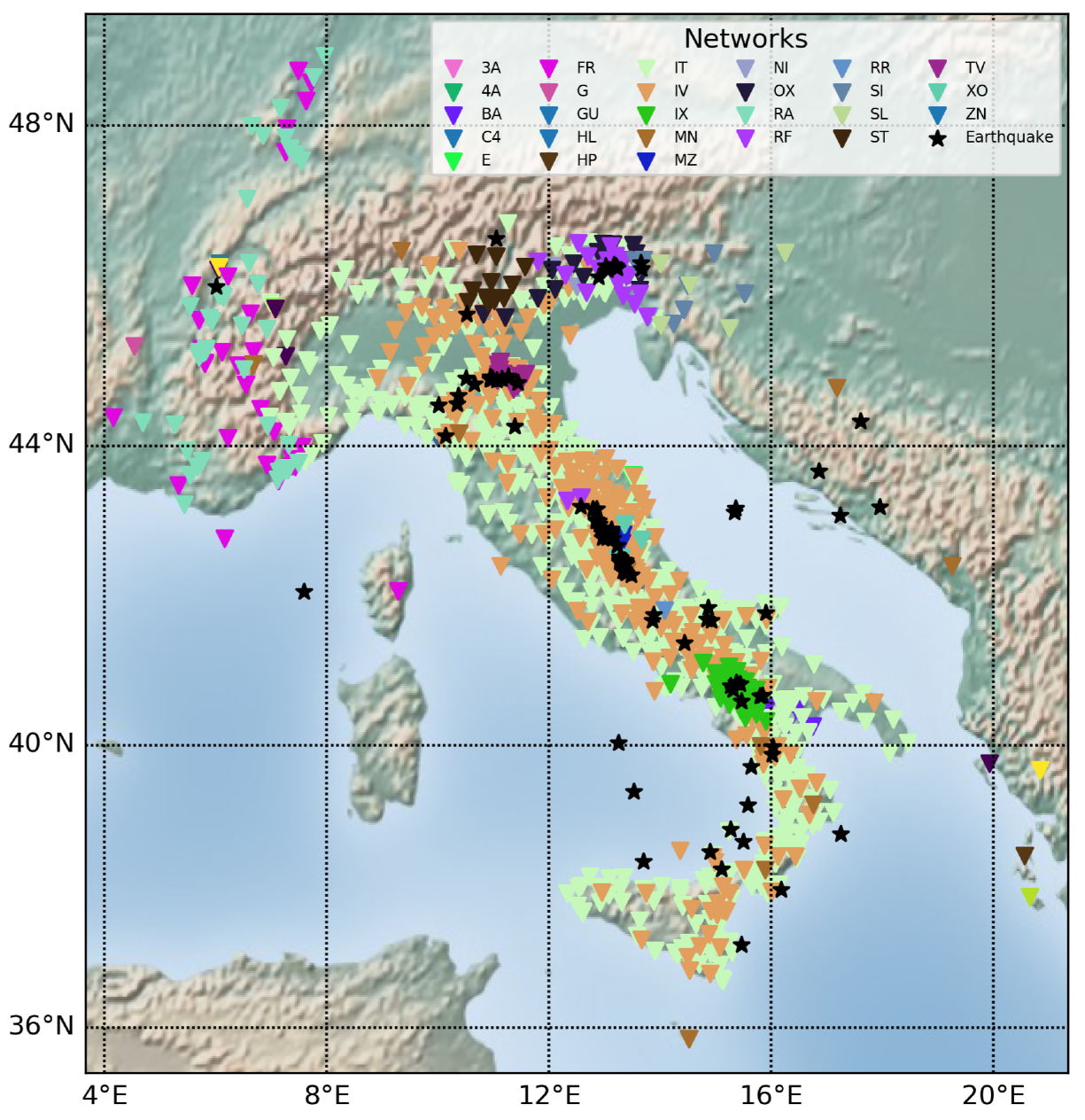
2. Data
3. Method
Determination of Impulsive Signals
4. Results
4.1. Friuli Earthquakes (IT-1976-0025, IT-1976-0027, IT-1976-0030) and Aftershocks
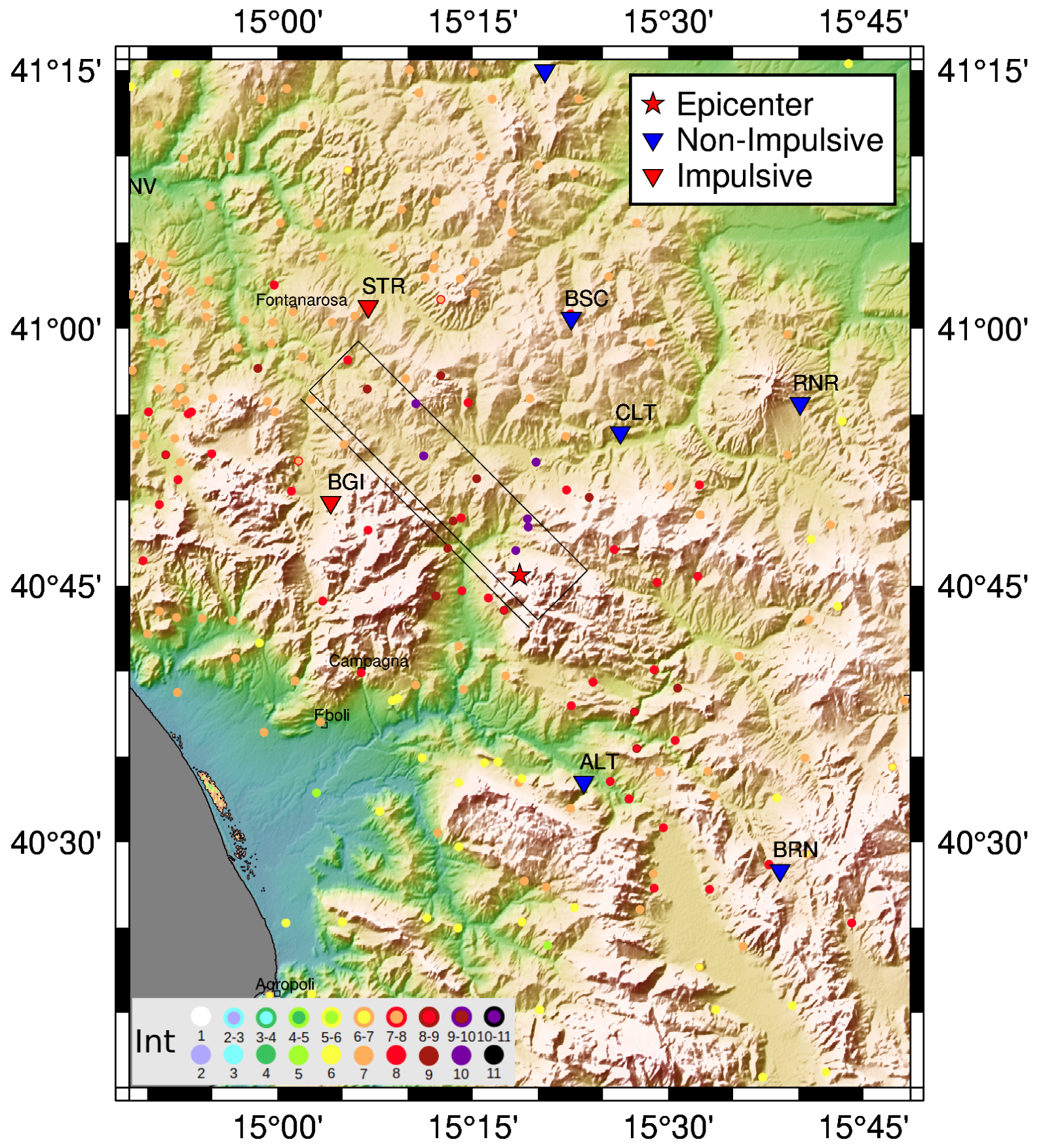
4.2. Irpinia Earthquake (IT-1980-0012) and Aftershocks
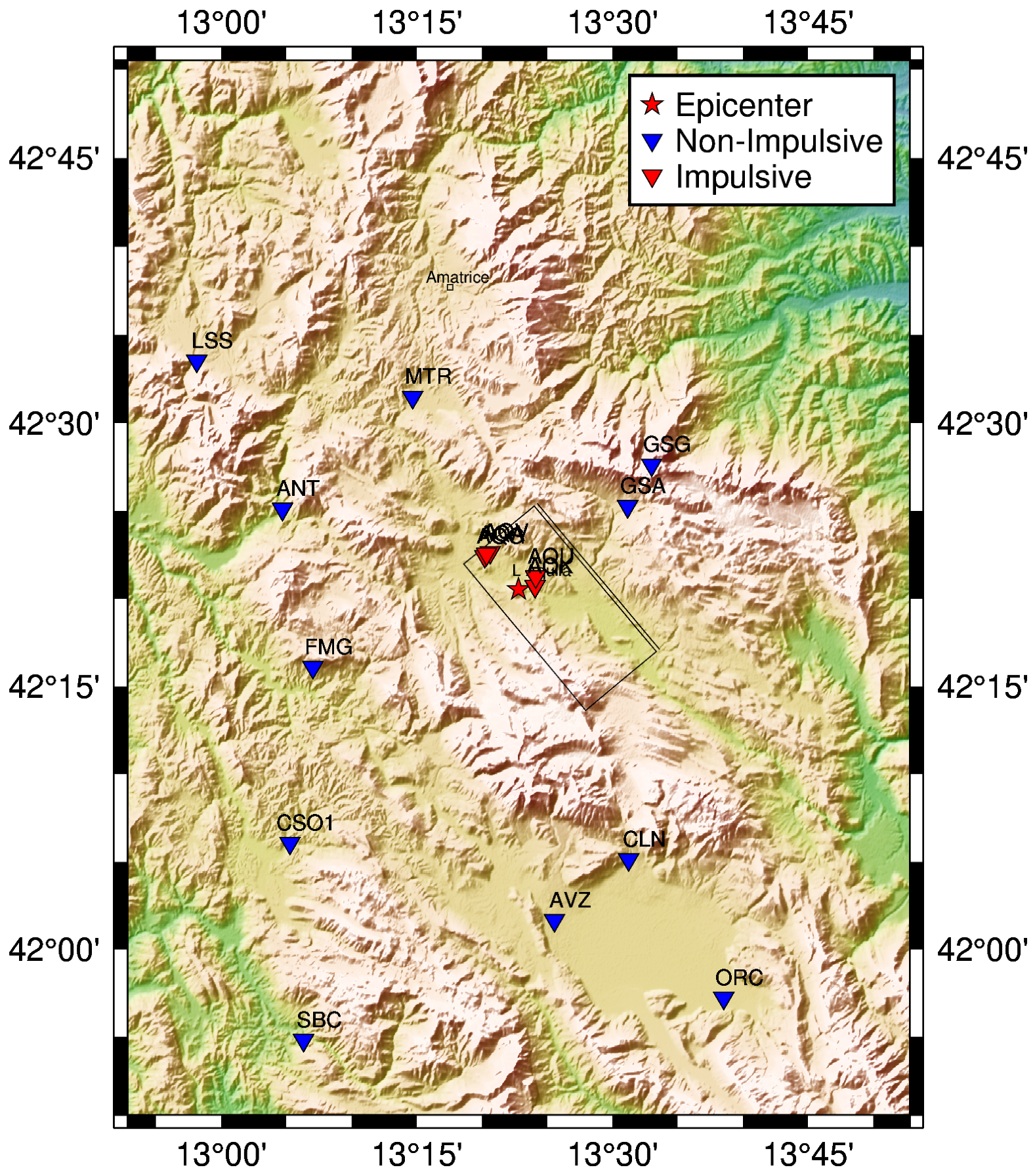
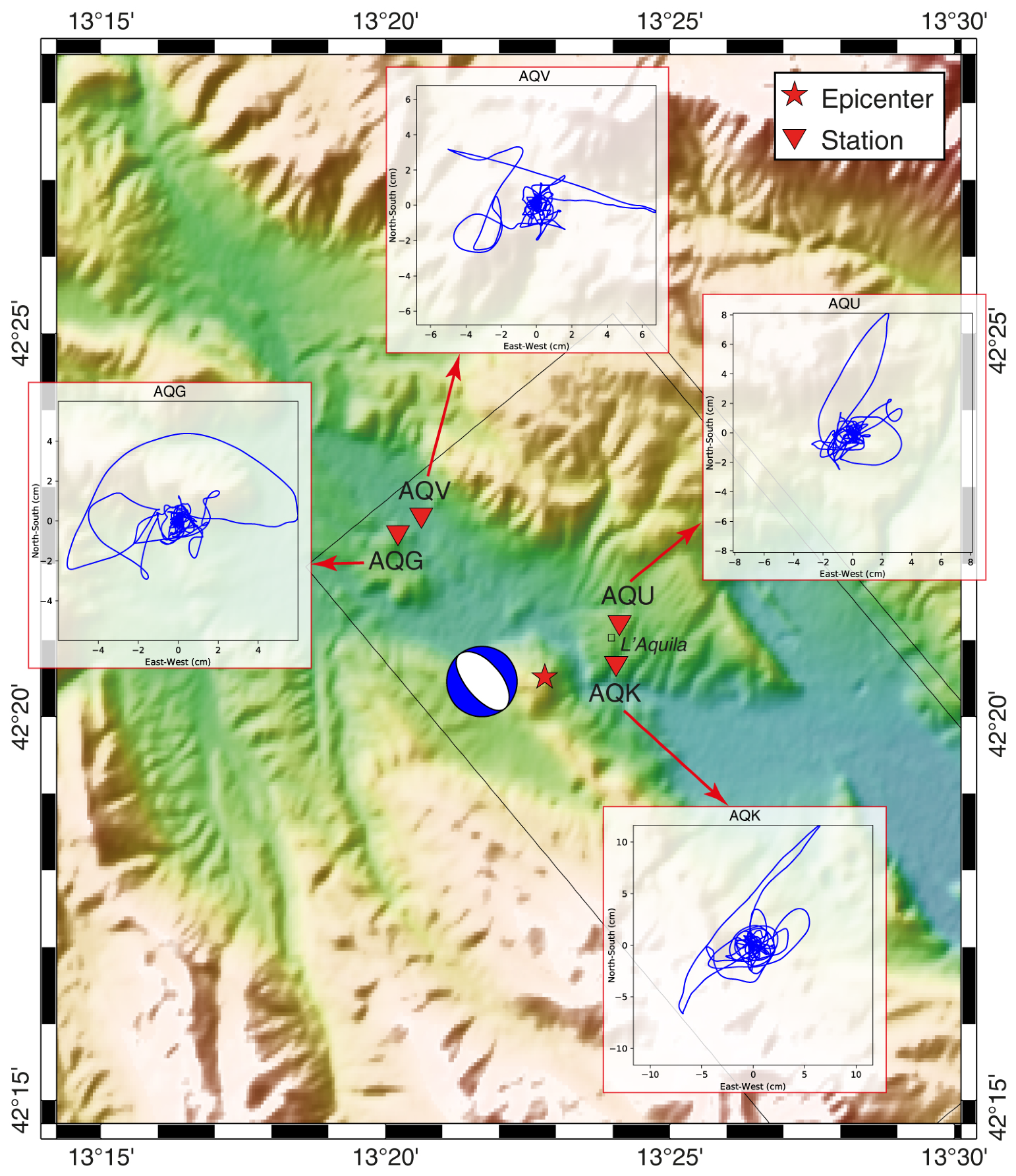
4.3. L’Aquila Earthquake (IT-2009-0009) and Aftershocks
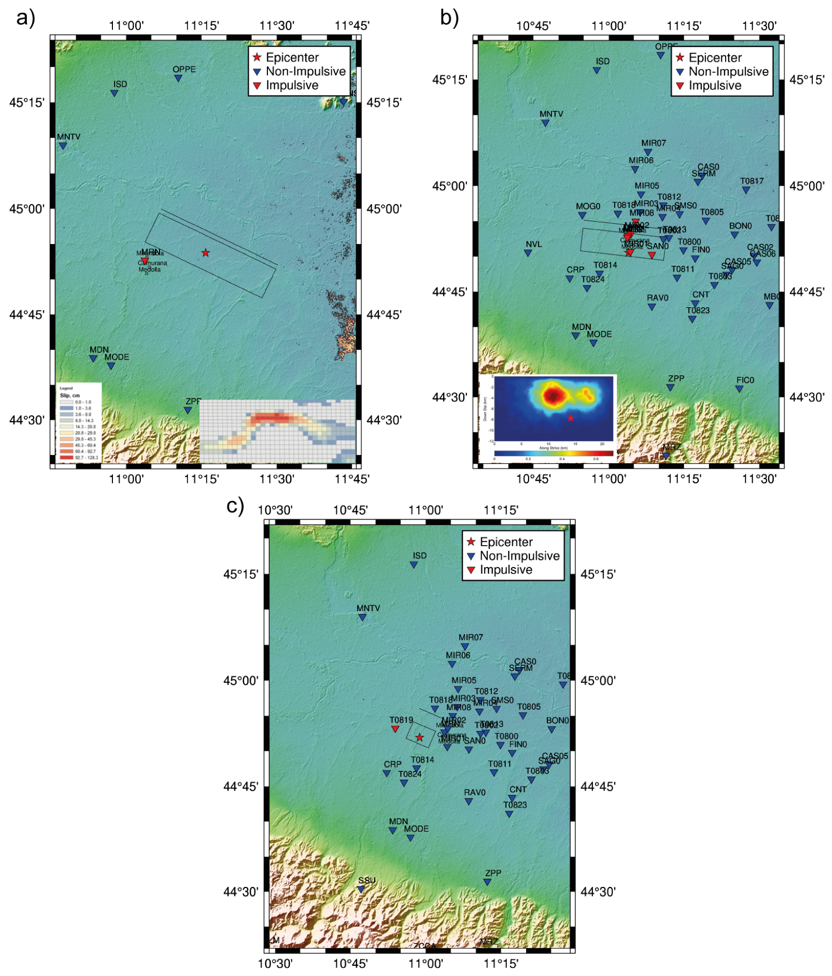
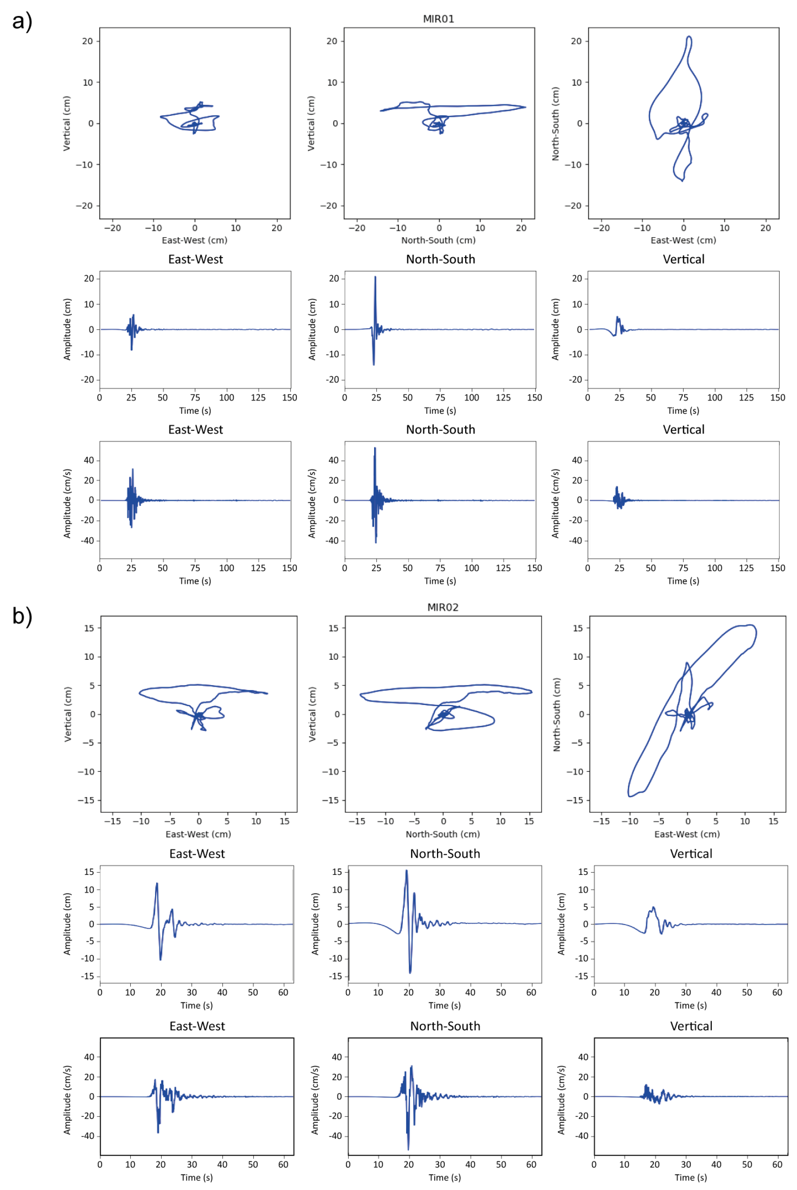
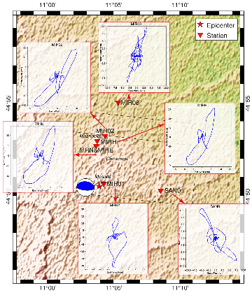
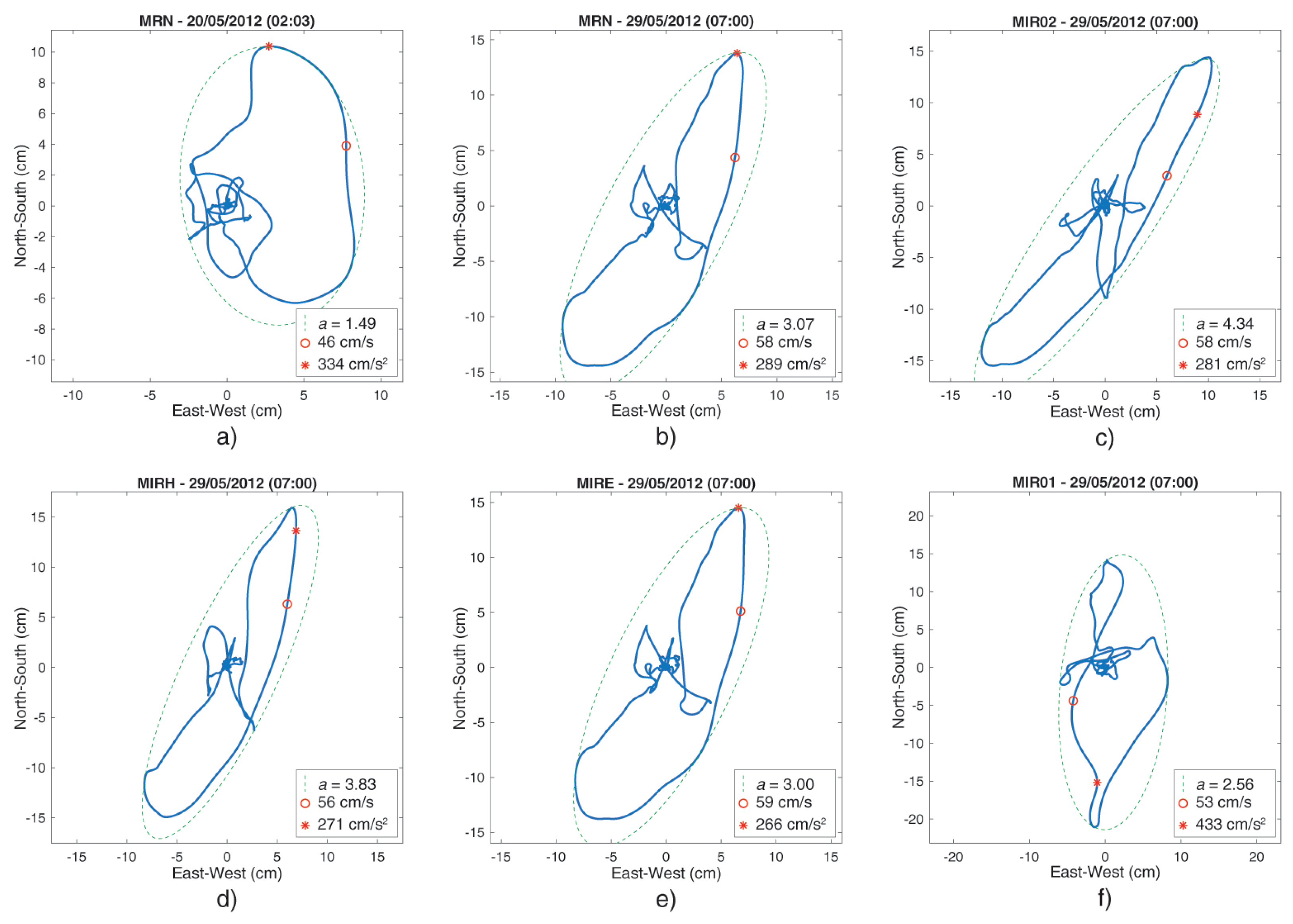
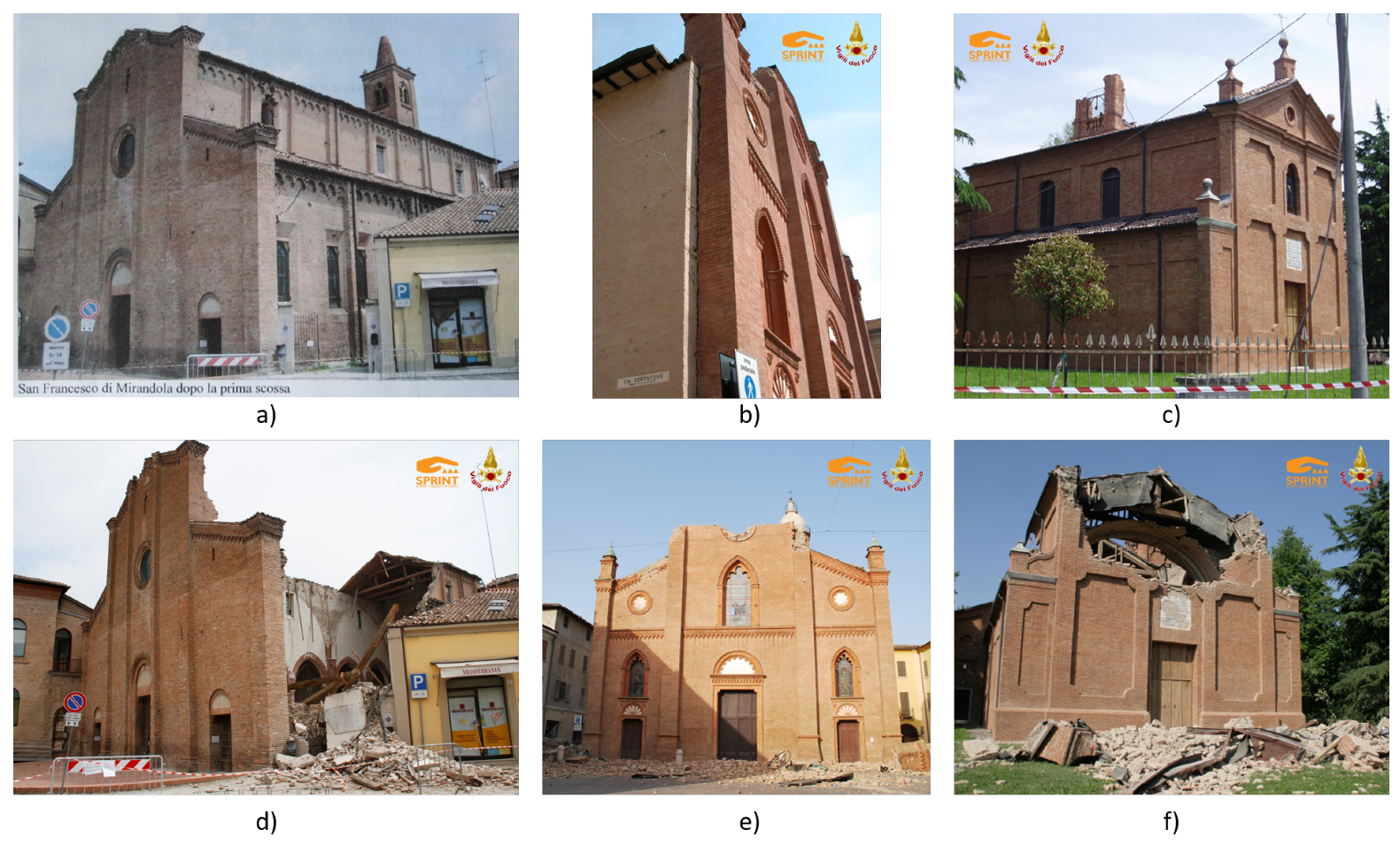
4.4. Emilia-Romagna Earthquakes (IT-2012-0008, IT-2012-0010, IT-2012-0011) and Aftershocks
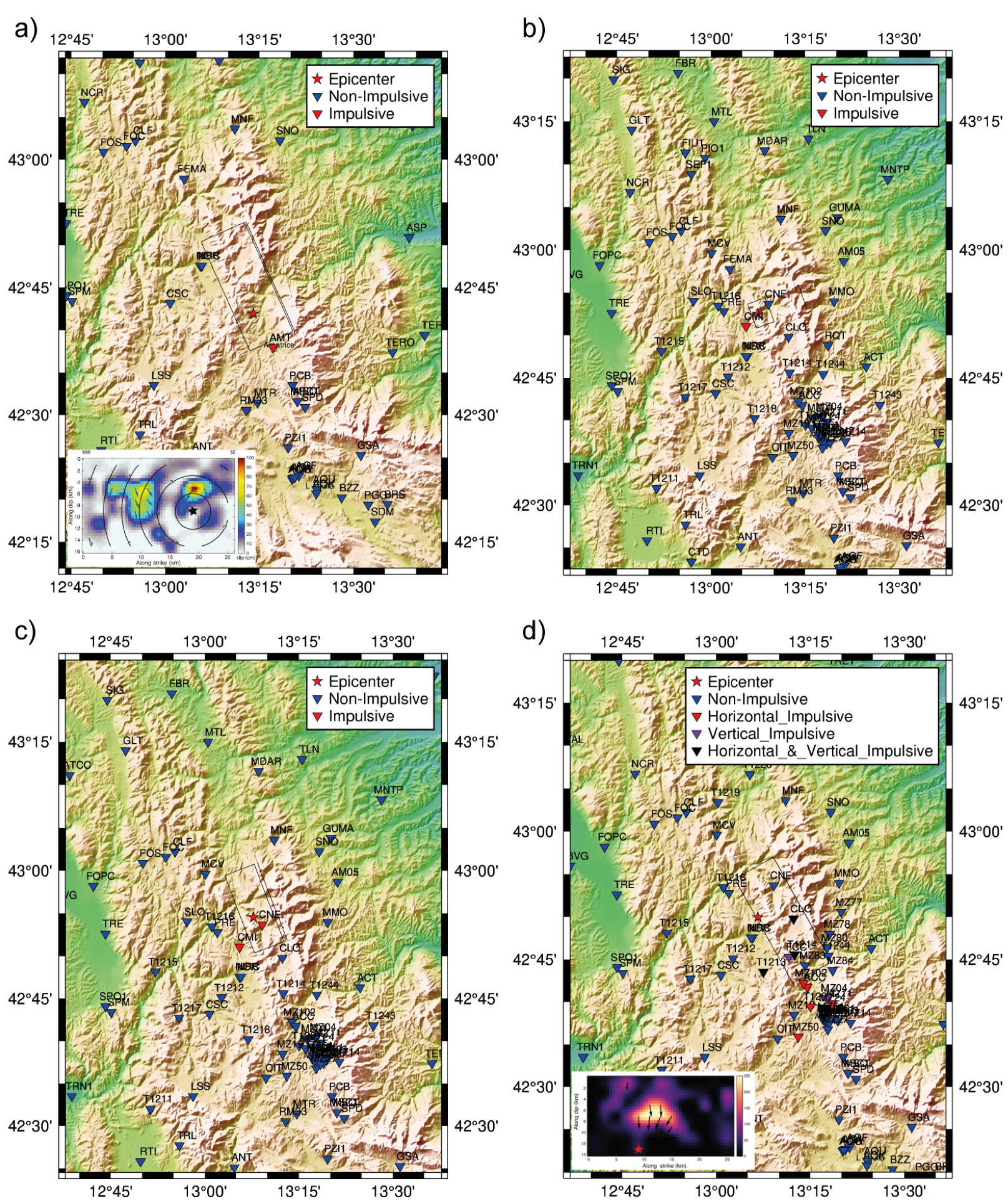
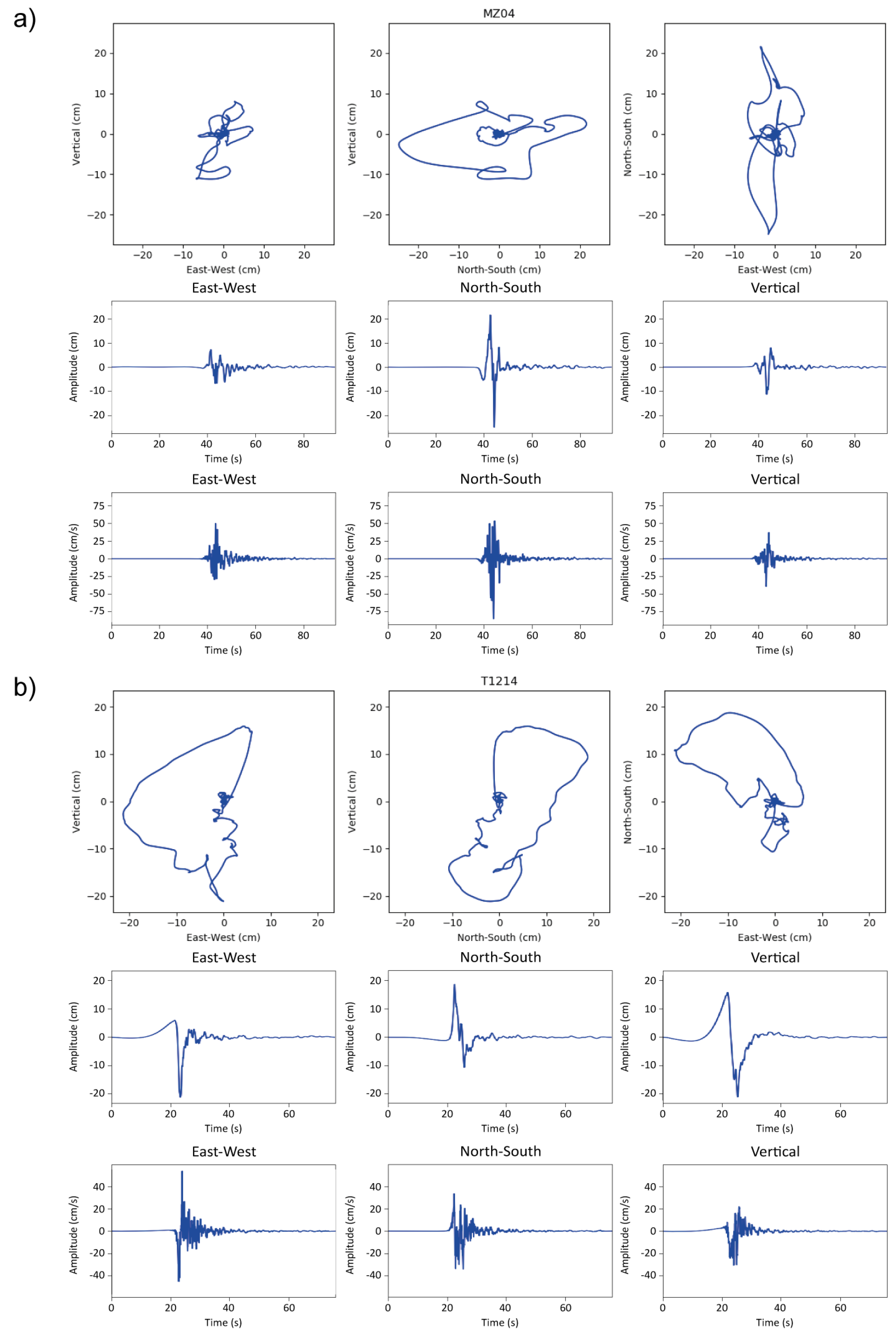
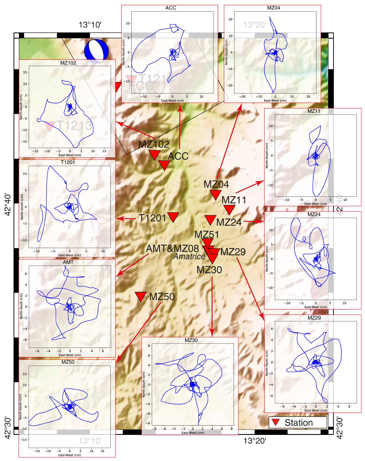
4.5. Amatrice Earthquakes (EMSC-20160824_0000006, EMSC-20161026_0000077, EMSC-20161026_0000095, EMSC-20161030_0000029) and Aftershocks
5. Discussion
- indicates that the signal can be described as SPD;
- can refer both to SPD and FBD;
- indicates that the signal can be described as FBD.
6. Conclusions
Supplementary Materials
Author Contributions
Funding
Data Availability Statement
Acknowledgments
Conflicts of Interest
Abbreviations
| CNVVF | Corpo Nazionale dei Vigili del Fuoco (The Italian National Fire Service) |
| FBD | Forward-Back-like Displacement |
| ITACA | ITalian ACcelerometric Archive |
| NCP | Nucleo Coordinamento opere Provvisionali (Coordination Unit for Shoring) |
| PC | Principal Component |
| PI | Pulse Indicator |
| PGV | Peak Ground Velocity |
| SPD | Spinning-like Displacement |
References
- Somerville, P.G.; Smith, N.F.; Graves, R.W.; Abrahamson, N.A. Accounting for near-fault rupture directivity effects in the development of design ground motions. ASME-PUBLICATIONS-PVP 1995, 319, 67–82. [Google Scholar]
- Bolt, B.A.; Abrahamson, N.A. 59 Estimation of strong seismic ground motions. Int. Geophys. 2003, 81, 983–1001. [Google Scholar] [CrossRef]
- Mavroeidis, G.P.; Papageorgiou, A.S. A mathematical representation of near-fault ground motions. Bull. Seismol. Soc. Am. 2003, 93, 1099–1131. [Google Scholar] [CrossRef]
- Somerville, P.G.; Smith, N.F.; Graves, R.W.; Abrahamson, N.A. Modification of Empirical Strong Ground Motion Attenuation Relations to Include the Amplitude and Duration Effects of Rupture Directivity. Seismol. Res. Lett. 1997, 68, 199–222. [Google Scholar] [CrossRef]
- Alavi, B.; Krawinkler, H. Behavior of moment-resisting frame structures subjected to near-fault ground motions. Earthq. Eng. Struct. Dyn. 2004, 33, 687–706. [Google Scholar] [CrossRef]
- Mavroeidis, G.; Dong, G.; Papageorgiou, A. Near-fault ground motions, and the response of elastic and inelastic single-degree-of-freedom (SDOF) systems. Earthq. Eng. Struct. Dyn. 2004, 33, 1023–1049. [Google Scholar] [CrossRef]
- Gillie, J.; Rodriguez-Marek, A.; McDaniel, C. Strength reduction factors for near-fault forward-directivity ground motions. Eng. Struct. 2010, 32, 273–285. [Google Scholar] [CrossRef]
- Hubbard, D.; Mavroeidis, G. Damping coefficients for near-fault ground motion response spectra. Soil Dyn. Earthq. Eng. 2011, 31, 401–417. [Google Scholar] [CrossRef]
- Champion, C.; Liel, A. The effect of near-fault directivity on building seismic collapse risk. Earthq. Eng. Struct. Dyn. 2012, 41, 1391–1409. [Google Scholar] [CrossRef]
- Kalkan, E.; Kunnath, S.K. Effects of fling step and forward directivity on seismic response of buildings. Earthq. Spectra 2006, 22, 367–390. [Google Scholar] [CrossRef]
- Grimaz, S.; Malisan, P. Near field domain effects and their consideration in the international and Italian seismic codes. Boll. Geofis. Teor. Appl. 2014, 55, 717–738. [Google Scholar] [CrossRef]
- Alonso-Rodríguez, A.; Miranda, E. Assessment of building behavior under near-fault pulse-like ground motions through simplified models. Soil Dyn. Earthq. Eng. 2015, 79, 47–58. [Google Scholar] [CrossRef]
- Cao, Y.; Meza-Fajardo, K.; Mavroeidis, G.; Papageorgiou, A. Effects of wave passage on torsional response of symmetric buildings subjected to near-fault pulse-like ground motions. Soil Dyn. Earthq. Eng. 2016, 88, 109–123. [Google Scholar] [CrossRef]
- Cao, Y.; Mavroeidis, G.; Meza-Fajardo, K.; Papageorgiou, A. Accidental eccentricity in symmetric buildings due to wave passage effects arising from near-fault pulse-like ground motions. Earthq. Eng. Struct. Dyn. 2017, 46, 2185–2207. [Google Scholar] [CrossRef]
- Iervolino, I.; Baltzopoulos, G.; Chioccarelli, E.; Suzuki, A. Seismic actions on structures in the near-source region of the 2016 central Italy sequence. Bull. Earthq. Eng. 2019, 17, 5429–5447. [Google Scholar] [CrossRef]
- Hall, J.F.; Heaton, T.H.; Halling, M.W.; Wald, D.J. Near-Source Ground Motion and its Effects on Flexible Buildings. Earthq. Spectra 1995, 11, 569–605. [Google Scholar] [CrossRef]
- Makris, N. Rigidity-plasticity-viscosity: Can electrorheological dampers protect base-isolated structures from near-source ground motions? Earthq. Eng. Struct. Dyn. 1997, 26, 571–591. [Google Scholar] [CrossRef]
- Mazza, F. Seismic demand of base-isolated irregular structures subjected to pulse-type earthquakes. Soil Dyn. Earthq. Eng. 2018, 108, 111–129. [Google Scholar] [CrossRef]
- Habib, A.; Houri, A.A.; Yildirim, U. Comparative study of base-isolated irregular RC structures subjected to pulse-like ground motions with low and high PGA/PGV ratios. Structures 2021, 31, 1053–1071. [Google Scholar] [CrossRef]
- Bhagat, S.; Wijeyewickrema, A.; Subedi, N. Influence of Near-Fault Ground Motions with Fling-Step and Forward-Directivity Characteristics on Seismic Response of Base-Isolated Buildings. J. Earthq. Eng. 2021, 25, 455–474. [Google Scholar] [CrossRef]
- Ucak, A.; Mavroeidis, G.; Tsopelas, P. Behavior of a seismically isolated bridge crossing a fault rupture zone. Soil Dyn. Earthq. Eng. 2014, 57, 164–178. [Google Scholar] [CrossRef]
- Yang, S.; Mavroeidis, G.; Ucak, A.; Tsopelas, P. Effect of ground motion filtering on the dynamic response of a seismically isolated bridge with and without fault crossing considerations. Soil Dyn. Earthq. Eng. 2017, 92, 183–191. [Google Scholar] [CrossRef]
- Falsone, G.; Recupero, A.; Spinella, N. Effects of near-fault earthquakes on existing bridge performances. J. Civ. Struct. Health Monit. 2020, 10, 165–176. [Google Scholar] [CrossRef]
- Yang, S.; Mavroeidis, G.; Ucak, A. Analysis of bridge structures crossing strike-slip fault rupture zones: A simple method for generating across-fault seismic ground motions. Earthq. Eng. Struct. Dyn. 2020, 49, 1281–1307. [Google Scholar] [CrossRef]
- Zhong, J.; Jiang, L.; Pang, Y.; Yuan, W. Near-fault seismic risk assessment of simply supported bridges. Earthq. Spectra 2020, 36, 1645–1669. [Google Scholar] [CrossRef]
- Madan, A.; Hashmi, A. Analytical prediction of the seismic performance of masonry infilled reinforced concrete frames subjected to near-field earthquakes. J. Struct. Eng. 2008, 134, 1569–1581. [Google Scholar] [CrossRef]
- Liossatou, E.; Fardis, M. Near-fault effects on residual displacements of RC structures. Earthq. Eng. Struct. Dyn. 2016, 45, 1391–1409. [Google Scholar] [CrossRef]
- Hamidi, H.; Karbassi, A.; Lestuzzi, P. Seismic response of RC buildings subjected to fling-step in the near-fault region. Struct. Concr. 2020, 21, 1919–1937. [Google Scholar] [CrossRef]
- Shahaki Kenari, M.; Celikag, M. Correlation of Ground Motion Intensity Measures and Seismic Damage Indices of Masonry-Infilled Steel Frames. Arab. J. Sci. Eng. 2019, 44, 5131–5150. [Google Scholar] [CrossRef]
- Bilgin, H.; Hysenlliu, M. Comparison of near and far-fault ground motion effects on low and mid-rise masonry buildings. J. Build. Eng. 2020, 30. [Google Scholar] [CrossRef]
- Augenti, N.; Parisi, F. Learning from Construction Failures due to the 2009 L’Aquila, Italy, Earthquake. J. Perform. Constr. Facil. 2010, 24, 536–555. [Google Scholar] [CrossRef]
- Kaplan, H.; Bilgin, H.; Yilmaz, S.; Binici, H.; Öztas, A. Structural damages of L’Aquila (Italy) earthquake. Nat. Hazards Earth Syst. Sci. 2010, 10, 499–507. [Google Scholar] [CrossRef]
- Carocci, C.F. Small centres damaged by 2009 L’Aquila earthquake: On site analyses of historical masonry aggregates. Bull. Earthq. Eng. 2012, 10, 45–71. [Google Scholar] [CrossRef]
- Ricci, P.; De Luca, F.; Verderame, G.M. 6th April 2009 L’Aquila earthquake, Italy: Reinforced concrete building performance. Bull. Earthq. Eng. 2011, 9, 285–305. [Google Scholar] [CrossRef]
- Brandonisio, G.; Lucibello, G.; Mele, E.; Luca, A.D. Damage and performance evaluation of masonry churches in the 2009 L’Aquila earthquake. Eng. Fail. Anal. 2013, 34, 693–714. [Google Scholar] [CrossRef]
- Grimaz, S.; Maiolo, A. The impact of the 6 April 2009 l’Aquila earthquake (Italy) on the industrial facilities and life lines. Considerations in terms of NaTech risk. Chem. Eng. Trans. 2010, 19, 279–284. [Google Scholar] [CrossRef]
- Cattari, S.; Degli Abbati, S.; Ferretti, D.; Lagomarsino, S.; Ottonelli, D.; Tralli, A. Damage assessment of fortresses after the 2012 Emilia earthquake (Italy). Bull. Earthq. Eng. 2014, 12, 2333–2365. [Google Scholar] [CrossRef]
- Lagomarsino, S. Damage assessment of churches after L’Aquila earthquake (2009). Bull. Earthq. Eng. 2012, 10, 73–92. [Google Scholar] [CrossRef]
- Parisi, F.; De Luca, F.; Petruzzelli, F.; De Risi, R.; Chioccarelli, E.; Iervolino, I. Field Inspection after the May 20th and 29th 2012 Emilia-Romagna Earthquakes; Italian Network of Earthquake Engineering University Laboratories: Naples, Italy, 2012. [Google Scholar]
- Sorrentino, L.; Liberatore, L.; Decanini, L.D.; Liberatore, D. The performance of churches in the 2012 Emilia earthquakes. Bull. Earthq. Eng. 2014, 12, 2299–2331. [Google Scholar] [CrossRef]
- Milani, G.; Valente, M. Failure analysis of seven masonry churches severely damaged during the 2012 Emilia-Romagna (Italy) earthquake: Non-linear dynamic analyses vs conventional static approaches. Eng. Fail. Anal. 2015, 54, 13–56. [Google Scholar] [CrossRef]
- Valente, M.; Barbieri, G.; Biolzi, L. Damage assessment of three medieval churches after the 2012 Emilia earthquake. Bull. Earthq. Eng. 2017, 15, 2939–2980. [Google Scholar] [CrossRef]
- Bournas, D.A.; Negro, P.; Taucer, F.F. Performance of industrial buildings during the Emilia earthquakes in Northern Italy and recommendations for their strengthening. Bull. Earthq. Eng. 2014, 12, 2383–2404. [Google Scholar] [CrossRef]
- Ercolino, M.; Magliulo, G.; Manfredi, G. Failure of a precast RC building due to Emilia-Romagna earthquakes. Eng. Struct. 2016, 118, 262–273. [Google Scholar] [CrossRef]
- Savoia, M.; Buratti, N.; Vincenzi, L. Damage and collapses in industrial precast buildings after the 2012 Emilia earthquake. Eng. Struct. 2017, 137, 162–180. [Google Scholar] [CrossRef]
- Grimaz, S.; Malisan, P. How could cumulative damage affect the macroseismic assessment? Bull. Earthq. Eng. 2016, 15, 1–17. [Google Scholar] [CrossRef]
- Sorrentino, L.; Cattari, S.; da Porto, F.; Magenes, G.; Penna, A. Seismic behaviour of ordinary masonry buildings during the 2016 central Italy earthquakes. Bull. Earthq. Eng. 2019, 17, 5583–5607. [Google Scholar] [CrossRef]
- Jain, A.; Acito, M.; Chesi, C. Seismic sequence of 2016–17: Linear and non-linear interpretation models for evolution of damage in San Francesco church, Amatrice. Eng. Struct. 2020, 211, 110418. [Google Scholar] [CrossRef]
- Masi, A.; Chiauzzi, L.; Santarsiero, G.; Manfredi, V.; Biondi, S.; Spacone, E.; Del Gaudio, C.; Ricci, P.; Manfredi, G.; Verderame, G.M. Seismic response of RC buildings during the Mw 6.0 August 24, 2016 Central Italy earthquake: The Amatrice case study. Bull. Earthq. Eng. 2019, 17, 5631–5654. [Google Scholar] [CrossRef]
- Baker, J.W. Quantitative Classification of Near-Fault Ground Motions Using Wavelet Analysis. Bull. Seismol. Soc. Am. 2007, 97, 1486–1501. [Google Scholar] [CrossRef]
- Shahi, S.K.; Baker, J.W. An Efficient Algorithm to Identify Strong-Velocity Pulses in Multicomponent Ground Motions. Bull. Seismol. Soc. Am. 2014, 104, 2456–2466. [Google Scholar] [CrossRef]
- Chang, Z.; Sun, X.; Zhai, C.; Zhao, J.X.; Xie, L. An improved energy-based approach for selecting pulse-like ground motions. Earthq. Eng. Struct. Dyn. 2016, 45, 2405–2411. [Google Scholar] [CrossRef]
- Ertuncay, D.; Costa, G. An alternative pulse classification algorithm based on multiple wavelet analysis. J. Seismol. 2019, 23, 929–942. [Google Scholar] [CrossRef]
- Somerville, P.G. Magnitude scaling of the near fault rupture directivity pulse. Phys. Earth Planet. Inter. 2003, 137, 201–212. [Google Scholar] [CrossRef]
- Bray, J.D.; Rodriguez-Marek, A. Characterization of forward-directivity ground motions in the near-fault region. Soil Dyn. Earthq. Eng. 2004, 24, 815–828. [Google Scholar] [CrossRef]
- Halldórsson, B.; Mavroeidis, G.P.; Papageorgiou, A.S. Near-fault and far-field strong ground-motion simulation for earthquake engineering applications using the specific barrier model. J. Struct. Eng. 2011, 137, 433–444. [Google Scholar] [CrossRef]
- Tang, Y.; Zhang, J. Response spectrum-oriented pulse identification and magnitude scaling of forward directivity pulses in near-fault ground motions. Soil Dyn. Earthq. Eng. 2011, 31, 59–76. [Google Scholar] [CrossRef]
- Cork, T.G.; Kim, J.H.; Mavroeidis, G.P.; Kim, J.K.; Halldorsson, B.; Papageorgiou, A.S. Effects of tectonic regime and soil conditions on the pulse period of near-fault ground motions. Soil Dyn. Earthq. Eng. 2016, 80, 102–118. [Google Scholar] [CrossRef]
- Sgobba, S.; Lanzano, G.; Pacor, F.; Felicetta, C. An Empirical Model to Account for Spectral Amplification of Pulse-Like Ground Motion Records. Geosciences 2021, 11, 15. [Google Scholar] [CrossRef]
- Fayjaloun, R.; Causse, M.; Voisin, C.; Cornou, C.; Cotton, F. Spatial Variability of the Directivity Pulse Periods Observed during an Earthquake. Bull. Seismol. Soc. Am. 2017, 107, 308–318. [Google Scholar] [CrossRef][Green Version]
- Iervolino, I.; Cornell, C.A. Probability of Occurrence of Velocity Pulses in Near-Source Ground Motions. Bull. Seismol. Soc. Am. 2008, 98, 2262–2277. [Google Scholar] [CrossRef]
- Ertuncay, D.; Costa, G. Determination of near-fault impulsive signals with multivariate naïve Bayes method. Nat. Hazards 2021, 1–18. [Google Scholar] [CrossRef]
- Luzi, L.; Puglia, R.; Russo, E.; D’Amico, M.; Felicetta, C.; Pacor, F.; Lanzano, G.; Çeken, U.; Clinton, J.; Costa, G.; et al. The engineering strong-motion database: A platform to access pan-European accelerometric data. Seismol. Res. Lett. 2016, 87, 987–997. [Google Scholar] [CrossRef]
- Pacor, F.; Paolucci, R.; Luzi, L.; Sabetta, F.; Spinelli, A.; Gorini, A.; Nicoletti, M.; Marcucci, S.; Filippi, L.; Dolce, M. Overview of the Italian strong motion database. Bull Earthq. Eng. 2011, 9, 1723–1739. [Google Scholar] [CrossRef]
- Rovida, A.; Locati, M.; Camassi, R.; Lolli, B.; Gasperini, P. The Italian earthquake catalogue CPTI15. Bull. Earthq. Eng. 2020, 18, 2953–2984. [Google Scholar] [CrossRef]
- Goldstein, P.; Dodge, D.; Firpo, M.; Minner, L. 85.5 SAC2000: Signal processing and analysis tools for seismologists and engineers. In International Geophysics; Elsevier: Amsterdam, The Netherlands, 2003; Volume 81, pp. 1613–1614. [Google Scholar] [CrossRef]
- Boore, D.M.; Watson-Lamprey, J.; Abrahamson, N.A. Orientation-independent measures of ground motion. Bull. Seismol. Soc. Am. 2006, 96, 1502–1511. [Google Scholar] [CrossRef]
- Paolucci, R.; Pacor, F.; Puglia, R.; Ameri, G.; Cauzzi, C.; Massa, M. Record processing in ITACA, the new Italian strong-motion database. In Earthquake Data in Engineering Seismology; Springer: Berlin/Heidelberg, Germany, 2011; pp. 99–113. [Google Scholar]
- Zhai, C.; Chang, Z.; Li, S.; Chen, Z.; Xie, L. Quantitative Identification of Near-Fault Pulse-Like Ground Motions Based on Energy. Bull. Seismol. Soc. Am. 2013, 103, 2591–2603. [Google Scholar] [CrossRef]
- Grimaz, S.; Malisan, P. Advancements from a posteriori studies on the damage to buildings caused by the 1976 Friuli earthquake (north-eastern Italy). Boll. Geofis. Teor. Appl. 2018, 59, 505–526. [Google Scholar] [CrossRef]
- Database of Individual Seismogenic Sources (DISS), Version 3.1. 1: A Compilation of Potential Sources for Earthquakes Larger Than M 5.5 in Italy and Surrounding Areas. 2010. Available online: http://diss.rm.ingv.it/diss/ (accessed on 25 May 2021).
- Uieda, L.; Tian, D.; Leong, W.J.; Toney, L.; Newton, T.; Wessel, P. PyGMT: A Python interface for the Generic Mapping Tools. 2020. Available online: https://www.pygmt.org/ (accessed on 25 May 2021).
- Ameri, G.; Emolo, A.; Pacor, F.; Gallovic, F. Ground-Motion Simulations for the 1980 M 6.9 Irpinia Earthquake (Southern Italy) and Scenario Events. Bull. Seismol. Soc. Am. 2011, 101, 1136–1151. [Google Scholar] [CrossRef]
- De Luca, G.; Marcucci, S.; Milana, G.; Sano, T. Evidence of low-frequency amplification in the city of L’Aquila, Central Italy, through a multidisciplinary approach including strong-and weak-motion data, ambient noise, and numerical modeling. Bull. Seismol. Soc. Am. 2005, 95, 1469–1481. [Google Scholar] [CrossRef]
- Akinci, A.; Malagnini, L.; Sabetta, F. Characteristics of the strong ground motions from the 6 April 2009 L’Aquila earthquake, Italy. Soil Dyn. Earthq. Eng. 2010, 30, 320–335. [Google Scholar] [CrossRef]
- Lanzo, G.; Pagliaroli, A. Seismic site effects at near-fault strong-motion stations along the Aterno River Valley during the Mw= 6.3 2009 L’Aquila earthquake. Soil Dyn. Earthq. Eng. 2012, 40, 1–14. [Google Scholar] [CrossRef]
- de Normalisation, C.C.E. Eurocode 8: Design of Structures for Earthquake Resistance-Part 1: General Rules, Seismic Actions and Rules for Buildings; European Committee for Standardization: Brussels, Belgium, 2004. [Google Scholar]
- Ameri, G.; Massa, M.; Bindi, D.; D’Alema, E.; Gorini, A.; Luzi, L.; Marzorati, S.; Pacor, F.; Paolucci, R.; Puglia, R.; et al. The 6 April 2009 Mw 6.3 L’Aquila (central Italy) earthquake: Strong-motion observations. Seismol. Res. Lett. 2009, 80, 951–966. [Google Scholar] [CrossRef]
- Ameri, G.; Gallovič, F.; Pacor, F. Complexity of the Mw 6.3 2009 L’Aquila (central Italy) earthquake: 2. Broadband strong motion modeling: L’AQUILA EARTHQUAKE-BROADBAND MODELING. J. Geophys. Res. Solid Earth 2012, 117. [Google Scholar] [CrossRef]
- Pezzo, G.; Merryman Boncori, J.P.; Tolomei, C.; Salvi, S.; Atzori, S.; Antonioli, A.; Trasatti, E.; Novali, F.; Serpelloni, E.; Candela, L.; et al. Coseismic Deformation and Source Modeling of the May 2012 Emilia (Northern Italy) Earthquakes. Seismol. Res. Lett. 2013, 84, 645–655. [Google Scholar] [CrossRef]
- Paolucci, R.; Mazzieri, I.; Smerzini, C. Anatomy of strong ground motion: Near-source records and three-dimensional physics-based numerical simulations of the Mw 6.0 2012 May 29 Po Plain Earthquake, Italy. Geophys. J. Int. 2015, 203, 2001–2020. [Google Scholar] [CrossRef]
- Kaklamanos, J.; Baise, L.G.; Boore, D.M. Estimating Unknown Input Parameters when Implementing the NGA Ground-Motion Prediction Equations in Engineering Practice. Earthq. Spectra 2011, 27, 1219–1235. [Google Scholar] [CrossRef]
- Ronald Abraham, J.; Lai, C.G.; Papageorgiou, A. Basin-effects observed during the 2012 Emilia earthquake sequence in Northern Italy. Soil Dyn. Earthq. Eng. 2015, 78, 230–242. [Google Scholar] [CrossRef]
- Dreger, D.; Hurtado, G.; Chopra, A.; Larsen, S. Near-field across-fault seismic ground motions. Bull. Seismol. Soc. Am. 2011, 101, 202–221. [Google Scholar] [CrossRef]
- Gallovič, F.; Valentová, L.; Ampuero, J.P.; Gabriel, A.A. Bayesian dynamic finite-fault inversion: 2. Application to the 2016 Mw 6.2 Amatrice, Italy, earthquake. J. Geophys. Res. Solid Earth 2019, 124, 6970–6988. [Google Scholar] [CrossRef]
- Spagnuolo, E.; Cirella, A.; Akinci, A. Investigating the effectiveness of rupture directivity during the August 24, 2016 Mw 6.0 central Italy earthquake. Ann. Geophys. 2016, 59. [Google Scholar] [CrossRef]
- D’Amico, M.; Felicetta, C.; Schiappapietra, E.; Pacor, F.; Gallovič, F.; Paolucci, R.; Puglia, R.; Lanzano, G.; Sgobba, S.; Luzi, L. Fling Effects from Near-Source Strong-Motion Records: Insights from the 2016 Mw 6.5 Norcia, Central Italy, Earthquake. Seismol. Res. Lett. 2019, 90, 659–671. [Google Scholar] [CrossRef]
- Tinti, E.; Scognamiglio, L.; Michelini, A.; Cocco, M. Slip heterogeneity and directivity of the ML 6.0, 2016, Amatrice Earthq. Estim. Rapid Finite-Fault Inversion: Rupture Process 2016 Amatrice Event. Geophys. Res. Lett. 2016, 43, 10745–10752. [Google Scholar] [CrossRef]
- Chiaraluce, L.; Di Stefano, R.; Tinti, E.; Scognamiglio, L.; Michele, M.; Casarotti, E.; Cattaneo, M.; De Gori, P.; Chiarabba, C.; Monachesi, G.; et al. The 2016 Central Italy Seismic Sequence: A First Look at the Mainshocks, Aftershocks, and Source Models. Seismol. Res. Lett. 2017, 88, 757–771. [Google Scholar] [CrossRef]
- Rodriguez-Marek, A.; Bray, J. Seismic site response for near-fault forward directivity ground motions. J. Geotech. Geoenviron. Eng. 2006, 132, 1611–1620. [Google Scholar] [CrossRef]
- Moshtagh, N. Minimum Volume Enclosing Ellipsoid. MATLAB Central File Exchange. 2021. Available online: https://www.mathworks.com/matlabcentral/fileexchange/9542-minimum-volume-enclosing-ellipsoid (accessed on 25 May 2021).
- Ahipaşaoğlu, S. Fast algorithms for the minimum volume estimator. J. Glob. Optim. 2015, 62, 351–370. [Google Scholar] [CrossRef]
- QGIS Development Team. QGIS Geographic Information System. 2009. Available online: https://qgis.org/ (accessed on 25 May 2021).
- Grimaz, S.; Malisan, P.; Bolognese, C.; Ponticelli, L.; Cavriani, M.; Mannino, E.; Munaro, L. The short-term countermeasures system of the Italian national fire service for post-earthquake response. Boll. Geofis. Teor. Appl. 2016, 57, 161–182. [Google Scholar] [CrossRef]
- Istituto Nazionale di Geofisica e Vulcanologia (INGV); Istituto di Geologia Ambientale e Geoingegneria (CNR-IGAG); Istituto per la Dinamica dei Processi Ambientali (CNR-IDPA); Istituto di Metodologie per L’Analisi Ambientale (CNR-IMAA); Agenzia Nazionale per le nuove tecnologie, L’energia e lo Sviluppo Economico Sostenibile (ENEA). Rete del Centro di Microzonazione Sismica (CentroMZ), Sequenza Sismica del 2016 in Italia Centrale. 2018. Available online: https://www.fdsn.org/networks/detail/3A_2016 (accessed on 25 May 2021). [CrossRef]
- Istituto Nazionale Di Geofisica E Vulcanologia (INGV). Emersito Seismic Network for Site Effect Studies in L’Aquila Town (Central Italy). 2009. Available online: https://www.fdsn.org/networks/detail/4A_2009/ (accessed on 25 May 2021).
- RESIF. RESIF-RLBP French Broad-Band Network, RESIF-RAP Strong Motion Network and Other Seismic Stations in Metropolitan France. 1995. Available online: https://www.fdsn.org/networks/detail/FR/ (accessed on 25 May 2021).
- Institut De Physique Du Globe De Paris (IPGP); Ecole Et Observatoire Des Sciences De La Terre De Strasbourg (EOST). GEOSCOPE, French Global Network of Broad Band Seismic Stations. 1982. Available online: https://www.fdsn.org/networks/detail/G/ (accessed on 25 May 2021).
- University of Genova. Regional Seismic Network of North Western Italy. 1967. Available online: https://www.fdsn.org/networks/detail/GU/ (accessed on 25 May 2021).
- National Observatory of Athens. National Observatory of Athens Seismic Network. 1997. Available online: https://www.fdsn.org/networks/detail/HL/ (accessed on 25 May 2021).
- University of Patras. PSLNET, Permanent Seismic Network Operated by the University of Patras, Greece. 2000. Available online: https://www.fdsn.org/networks/detail/HP/ (accessed on 25 May 2021).
- Presidency of Counsil of Ministers-Civil Protection Department. Italian Strong Motion Network. 1972. Available online: https://www.fdsn.org/networks/detail/IT/ (accessed on 25 May 2021).
- INGV Seismological Data Centre. Rete Sismica Nazionale (RSN). 1997. Available online: https://www.fdsn.org/networks/detail/IV/ (accessed on 25 May 2021).
- MedNet Project Partner Institutions. Mediterranean Very Broadband Seismographic Network (MedNet). 1988. Available online: https://www.fdsn.org/networks/detail/MN/ (accessed on 25 May 2021).
- Priolo, E.; Laurenzano, G.; Barnaba, C.; Bernardi, P.; Moratto, L.; Spinelli, A. OASIS: The OGS archive system of instrumental seismology. Seismol. Res. Lett. 2015, 86, 978–984. [Google Scholar] [CrossRef][Green Version]
- Istituto Nazionale di Oceanografia e di Geofisica Sperimentale (OGS) and University of Trieste. North-East Italy Broadband Network. 2002. Available online: https://www.fdsn.org/networks/detail/NI/ (accessed on 25 May 2021).
- OGS. North-East Italy Seismic Network. 2016. Available online: https://www.fdsn.org/networks/detail/OX/ (accessed on 25 May 2021). [CrossRef]
- RESIF. RESIF-RAP French Accelerometric Network. 1995. Available online: https://www.fdsn.org/networks/detail/RA/ (accessed on 25 May 2021).
- University of Trieste. Friuli Venezia Giulia Accelerometric Network. 1993. Available online: https://www.fdsn.org/networks/detail/RF/ (accessed on 25 May 2021).
- Slovenian Environment Agency. Seismic Network of the Republic of Slovenia. 2001. Available online: https://www.fdsn.org/networks/detail/SL/ (accessed on 25 May 2021).
- Geological Survey-Provincia Autonoma Di Trento. Trentino Seismic Network. 1981. Available online: https://www.fdsn.org/networks/detail/ST/ (accessed on 25 May 2021).
- EMERSITO Working Group. Rete sismica del gruppo EMERSITO, Sequenza Sismica del 2016 in Italia Centrale. 2018. Available online: https://www.fdsn.org/networks/detail/XO_2016/ (accessed on 25 May 2021). [CrossRef]


| ITACA_ID | Shahi and Baker [51] | Chang et al. [52] | Ertuncay and Costa [53] | ||
|---|---|---|---|---|---|
| Horizontal | Vertical | Horizontal | Vertical | ||
| IT-1976-0025 | 2 | 1 | 0 | 1 | 0 |
| IT-1976-0027 | 1 | 1 | 0 | 1 | 0 |
| IT-1976-0030 | 1 | 1 | 0 | 1 | 0 |
| IT-1980-0012 | 2 | 3 | 0 | 3 | 0 |
| IT-2009-0009 | 4 | 6 | 0 | 6 | 0 |
| IT-2012-0008 | 1 | 2 | 0 | 2 | 0 |
| IT-2012-0010 | 1 | 2 | 0 | 2 | 0 |
| IT-2012-0011 | 6 | 9 | 0 | 9 | 0 |
| IT-2012-0012 | 2 | 1 | 0 | 1 | 0 |
| EMSC-20160824_0000006 | 2 | 2 | 1 | 1 | 1 |
| EMSC-20161026_0000077 | 1 | 1 | 0 | 1 | 0 |
| EMSC-20161026_0000095 | 1 | 2 | 0 | 2 | 0 |
| EMSC-20161030_0000029 | 5 | 17 | 8 | 14 | 7 |
Publisher’s Note: MDPI stays neutral with regard to jurisdictional claims in published maps and institutional affiliations. |
© 2021 by the authors. Licensee MDPI, Basel, Switzerland. This article is an open access article distributed under the terms and conditions of the Creative Commons Attribution (CC BY) license (https://creativecommons.org/licenses/by/4.0/).
Share and Cite
Ertuncay, D.; Malisan, P.; Costa, G.; Grimaz, S. Impulsive Signals Produced by Earthquakes in Italy and Their Potential Relation with Site Effects and Structural Damage. Geosciences 2021, 11, 261. https://doi.org/10.3390/geosciences11060261
Ertuncay D, Malisan P, Costa G, Grimaz S. Impulsive Signals Produced by Earthquakes in Italy and Their Potential Relation with Site Effects and Structural Damage. Geosciences. 2021; 11(6):261. https://doi.org/10.3390/geosciences11060261
Chicago/Turabian StyleErtuncay, Deniz, Petra Malisan, Giovanni Costa, and Stefano Grimaz. 2021. "Impulsive Signals Produced by Earthquakes in Italy and Their Potential Relation with Site Effects and Structural Damage" Geosciences 11, no. 6: 261. https://doi.org/10.3390/geosciences11060261
APA StyleErtuncay, D., Malisan, P., Costa, G., & Grimaz, S. (2021). Impulsive Signals Produced by Earthquakes in Italy and Their Potential Relation with Site Effects and Structural Damage. Geosciences, 11(6), 261. https://doi.org/10.3390/geosciences11060261