Article

3D Probabilistic Modelling and Uncertainty Analysis of Glacial and Post-Glacial Deposits of the City of Saguenay, Canada

1
Département des Sciences Appliquées, Université du Québec à Chicoutimi, Saguenay, QC G7H 2B1, Canada
2
Geological Survey of Canada, Quebec City, QC G1K 9A9, Canada
*
Author to whom correspondence should be addressed.
Geosciences 2021, 11(5), 204; https://doi.org/10.3390/geosciences11050204
Submission received: 26 March 2021 / Revised: 21 April 2021 / Accepted: 25 April 2021 / Published: 7 May 2021
(This article belongs to the Special Issue Geospatial Analysis for Disaster Risk Monitoring and Assessment)

Abstract

:
Knowledge of the stratigraphic architecture and geotechnical properties of surficial soil sediments is essential for geotechnical risk assessment. In the Saguenay study area, the Quaternary deposits consist of a basal till layer and heterogeneous post-glacial deposits. Considering the stratigraphic setting and soil type heterogeneity, a multistep stochastic methodology is developed for 3D geological modelling and quantification of the associated uncertainties. This methodology is adopted for regional studies and involves geostatistical interpolation and simulation methods. Empirical Bayesian kriging (EBK) is applied to generate the bedrock topography map and determine the thickness of the till sediments and their uncertainties. The locally varying mean and variance of the EBK method enable accounting for data complexity and moderate nonstationarity. Sequential indicator simulation is then performed to determine the occurrence probability of the discontinuous post-glacial sediments (clay, sand and gravel) on top of the basal till layer. The individual thickness maps of the discontinuous soil layers and uncertainties are generated in a probabilistic manner. The proposed stochastic framework is suitable for heterogeneous soil deposits characterised with complex surface and subsurface datasets.

1. Introduction

The soil stratigraphy and geotechnical characteristics are important factors in geotechnical risk evaluations over a region. The two factors and their uncertainties are key elements, especially for probabilistic seismic risk assessment. The regional properties of soil deposits are heterogeneous due to the differences in deposition geometry and process. Soil heterogeneity is attributed to two main sources: one is rooted in the lithology and the other is the inherent spatial soil variability [1]. The so-called lithological (soil type) heterogeneity is related to the substantial differences in the mineralogy, grain size and others, within a relatively uniform soil mass. This heterogeneity is qualified using descriptive terms (i.e., soil types), such as sand, clay and stiff/soft soil layers. The second source of heterogeneity is rooted in the inherent spatial soil variability, which modifies the spatial variation of soil properties due to different deposition conditions and different loading histories [1].
The spatial variation of soil properties has been modelled using random field theory, where the spatial variation of a given soil unit is decomposed into a deterministic trend function and residuals [2,3,4,5]. Residuals represent the inherent spatial soil variability described by the coefficient of variation and the scale of fluctuation [3]. Using this approach, predictions are made separately for the trend and the residuals of geotechnical quantitative parameters (shear strength, cone resistance, shear modulus, etc.). Recently, some methods have been developed to model the random field directly from sparse and nonstationary data [6,7]. In soil and rock engineering practices, investigations use geostatistical techniques to estimate soil (or rock) geotechnical/geomechanical properties and capture the heterogeneity [8,9,10,11].
In seismic hazard assessment, local soil conditions tend to modify the amplitude and frequency content of the incoming seismic waves. This condition is known as the site effect, which depends on geotechnical (soil type, shear modulus, damping ratio, etc.) and geometrical (3D stratigraphy, basin topography, soil thickness, etc.) properties of the soil deposits. A 3D geological model offers solutions to determine the geometrical properties and provides a basis for the spatial prediction of geotechnical properties, particularly the soil shear wave velocity (Vs) [12]. A 3D model helps determine the seismic site parameters, including the average Vs value of the top 30 m of soil (Vs,30), the average Vs of all of the soil deposits (Vs,avg) and the fundamental site period (T0) or frequency (f0) [13,14]. In Eastern Canada, Rosset et al. [15] developed three different models for the Montreal region using predictive equations for Vs as a function of depth: a single-layer model based on the total thickness of soft soils, a four-layer model based on geological and geotechnical information from borehole data and a composite model that included the characteristics of the two former models. Nastev et al. [16] in the Ottawa and St. Lawrence Valleys and Foulon et al. [17] in the Saguenay City region assigned a typical Vs depth function for post-glacial sediments and a single Vs value to glacial sediments and bedrock units. These studies used a deterministic 3D geological model for mapping the spatial distribution of Vs,avg and T 0 . They analysed the uncertainty propagated to site parameters using the first-order, second-moment approach, and they considered only the statistical uncertainty related to the Vs of soil deposits. This approach ignores the spatial uncertainties related to the 3D geological model. Considering the uncertainties related to the type and thickness of the soil layers certainly helps the development of reliable seismic hazard maps.
This study aims to develop a methodology for probabilistic regional 3D modelling of soil deposits by considering soil type heterogeneity as the main source of uncertainty. This methodology is adopted for regional studies and involves stochastic interpolation and simulation methods. The capacities and advantages of the interpolation and geostatistical methods applied in each step are discussed. The territory of Saguenay City is used as a case study for the application of the methodology. Firstly, empirical Bayesian kriging (EBK) is tested and validated to determine the bedrock topography map in terms of the total soil thickness and the thickness of the till layer, that is, the basal glacial sediments. Available surficial geological maps, borehole logs, rock outcrops (zero soil thickness) and shallow till data are used in the interpolation processes. Secondly, sequential indicator simulation (SIS) is conducted to predict the occurrence probability of the discontinuous post-glacial soil layers on top of the till layer (e.g., clay, sand and gravel). Finally, the estimated probabilities are applied to determine the consistent spatial distribution of discontinuous soil units, the thickness maps and the associated uncertainties.

2. Methodology

With the rapid development of computational power and probabilistic methods, developing 3D geological models from borehole data and providing valuable insights into many engineering problems that traditionally rely on 1D and 2D assumptions, such as continuous stratigraphic layers simplified in the geological sections, are possible. The proposed methodology is adopted for regional study areas with variable soil thickness of more than 100 m in which a basal layer overlies the bedrock. The methodology is implemented in three phases (Figure 1): (I) data preparation, (II) mapping of bedrock and basal soil topography and (III) developing the probabilistic 3D geological model.
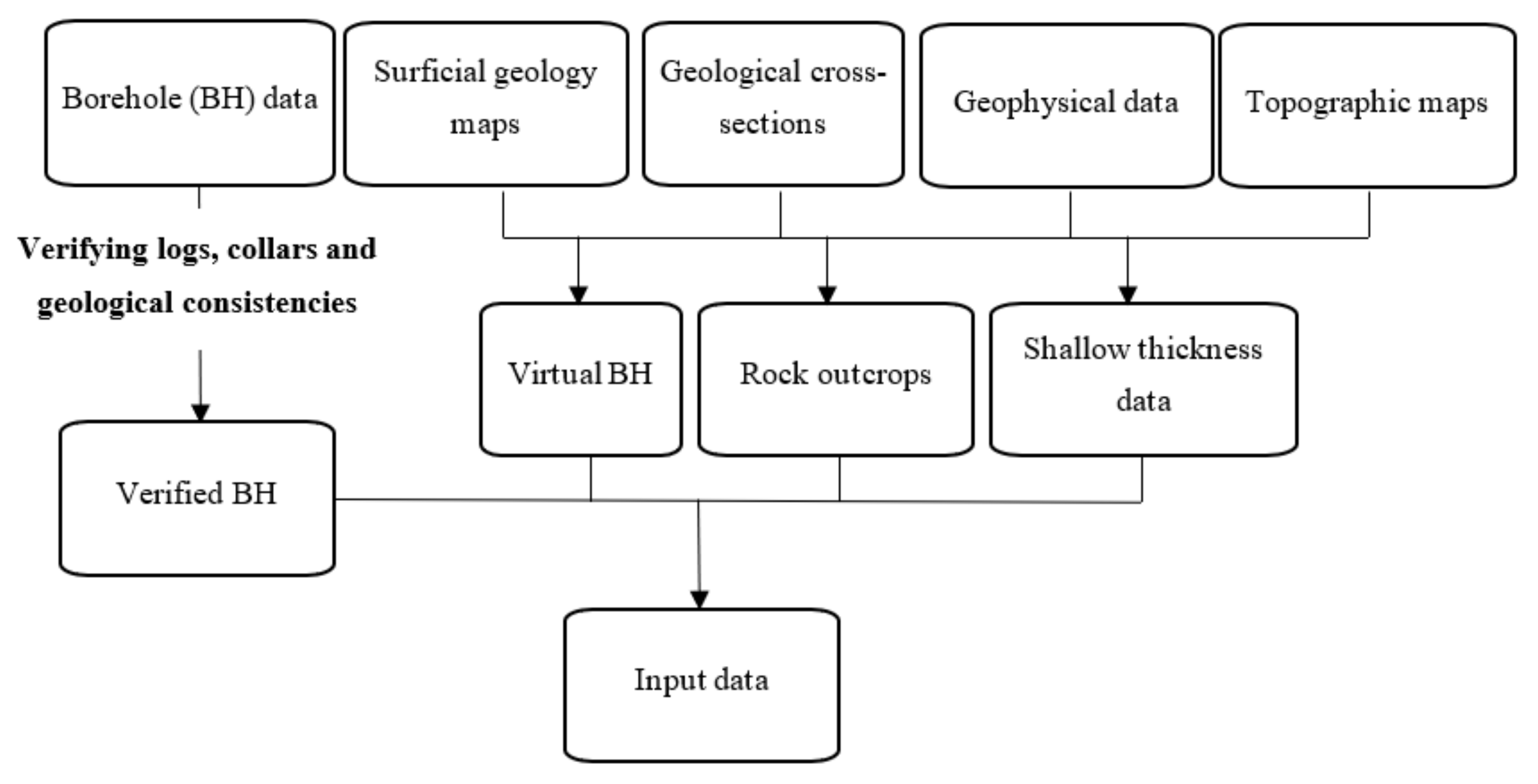
The data preparation step (Figure 2) relies on the acquisition of available data from various sources of information, as discussed below. Following the integration of the available data, the next step in this phase is data verification. It is performed by examining the consistency between borehole logs and geological maps and cross-sections, and between borehole collars and topographic maps. The observation data are then divided into two groups: the soil thickness data represented with points (x, y and thickness) and the soil type data represented with 3D borehole data (x, y, z and soil units).
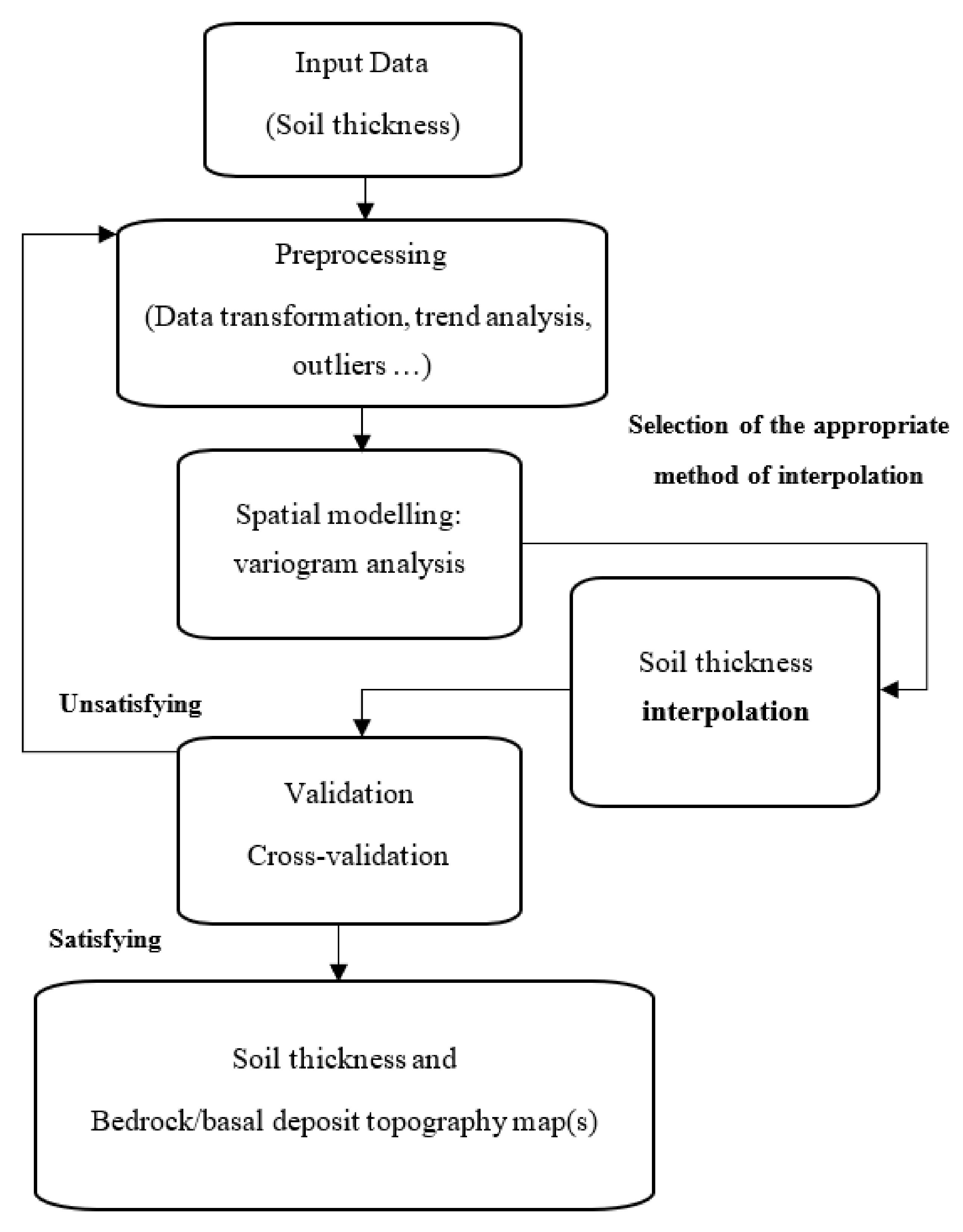
Next, a decision has to be made on the type of predictive model. For a stratigraphic soil unit that extends as a continuous layer, the thicknesses distribution can be modelled using spatial interpolation methods (Figure 3). In the study region described below, the till layer at the base of the Quaternary sequence is in contact with the bedrock and is assumed to be spread all over the territory underneath the recent soil layers. An appropriate spatial interpolation method should be selected in this phase corresponding to the preprocessing results. The trend and parameters, such as skewness or asymmetry of the probability distribution, and high or peak values, affect the stationarity and must be considered in choosing the appropriate geostatistical method (details can be found in Section 3 and Section 4). For a soil layer that is discontinuous laterally but maintains a vertical relationship with other layers, a random function approach using geostatistical simulation is used; this condition is the case for the sand and clay layers in the study region described below.
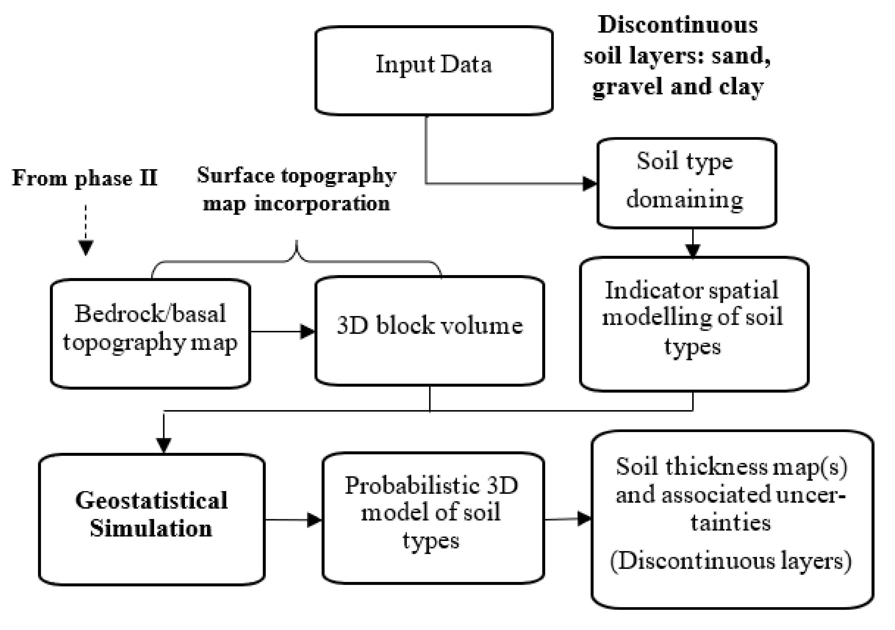
Multiple realisations of discontinuous soil types are generated using geostatistical simulation. These realisations can then provide the occurrence probability of discontinuous soil layers. The resulting probability values are used to create thickness maps of discontinuous soil layers and their associated uncertainties at unsampled locations (Figure 4).
The development of a probabilistic 3D geological model must use a spatial prediction approach that considers the uncertainties in the spatial variation models and in the ensuing stochastic simulation. This interpolation approach uses a geostatistical method that is presented in the following section.

3. Applied Geostatistical Methods

3.1. Spatial Interpolation

Appropriate prediction methods are required for a realistic reconstruction of the soil heterogeneity over a region with a complex 3D soil deposit architecture, relatively sparse field observations and datasets with clustered sampling patterns. The prediction methods for computing spatial data fall into two broad categories: deterministic and stochastic [18]. Deterministic predictions are obtained by using mathematical functions with known sample points. Stochastic methods associate the distribution of unknown values with a similar known distribution and can quantify the uncertainty associated with the interpolated values; this capability makes them superior to the deterministic approaches. Stochastic methods include those based on geostatistics and hybrid methods that consider machine learning [19]. In geostatistical methods, the principal concept of statistical inference is based on stationarity and requires the independency of the univariate and bivariate probability laws from the location; this concept is called second-order stationarity: the mean is constant and the variance only depends on separation h [20,21]. Given the data complexity of a study on a regional scale, the EBK method is selected to overcome the potential of the nonstationarity of data, automate the fitting of variograms and solve the kriging models. The process consists of: (i) estimation of a semivariogram model on the basis of the input data, (ii) simulation of a new set of data from the semivariogram model, (iii) estimation of a new semivariogram model on the basis of the simulated dataset and (iv) calculation of a weight for the new model using Bayes’ rule. The repetition of the process results in a spectrum of semivariograms rather than a single one. Hence, the uncertainty introduced in the variogram arises from using a series of semivariogram models rather than a single one [22]. The automated simulation process facilitates the subsetting of data into large datasets typical for regional studies and helps achieve local stationarity in subareas where the dataset is a mixture distribution of high and low values. The EBK method is particularly efficient for spatial interpolation in large-scale studies and/or datasets with complexities [22,23,24].
In addition to the EBK method, the results are compared with the conventional deterministic interpolation method, triangulated irregular network (TIN). For an area in the same region of Eastern Canada as the present study, Chesnaux et al. [25] concluded that the expected values predicted with the TIN method are more accurate than the ordinary kriging method.

3.2. Spatial Variation

Spatial variation refers to the dissimilarity of the pairs of values of a random variable as a function of their distance [20]. Modelling the spatial variation assists in predicting the soil attributes at unsampled locations. In the present study, the spatial variation is determined for continuous (soil thickness) and categorical (soil units) variables. An experimental variogram, γ ^ h , is used to statistically determine the average dissimilarity between data separated by vector h [26] and is assumed as a measure of spatial variability.
γ ^ h = 1 2   N h α = 1 N h z u α z u α + h 2 ,
where z u α   and   N h are the values of the variable of interest at location uα and the number of data pairs within distance h in the respective direction. In practice, the tolerance for distance h and its direction is specified. The direction of the separation vectors becomes irrelevant when the directional tolerance increases sufficiently. An omnidirectional variogram is a useful starting tool for structural analysis and provides the prerequisite information for calculating the directional variograms, whilst a directional variogram reveals the anisotropy pattern and the direction of the maximum and minimum spatial continuities [20]. Equation (1) is applied for continuous variables, whilst an indicator variogram is calculated for categorical variables by substituting indicator data i u α ; k for K indicators as follows:
γ ^ I h ; k = 1 2   N h α = 1 N h i u α ; k i u α + h ; k 2 ,   k = 1 ,   ,   K .
With the determination of the standard variogram characteristics (i.e., range, sill and nugget effect), a theoretical model that best fits the experimental variogram is selected (e.g., spherical, exponential or Gaussian model).

3.3. Uncertainty of Spatial Interpolation

The usual approach to modelling kriging uncertainty applies the error variance of kriging as follows [20]:
σ ˜ k 2 = C ˜ 00 + i = 1 n j = 1 n w i w j C ˜ i j 2 i = 1 n w i C ˜ i 0 ,
where w i w j represents the kriging weights, C ˜ 00 is the variance of point values, C ˜ i j is the covariance between measured samples and C ˜ i 0 is the covariance between measured and unknown values.

3.4. Stochastic Simulation

The 3D model of categorical variables is constructed by applying deterministic or stochastic approaches. Deterministic modelling is highly dependent on expert judgment and is conducted by delineating the boundaries of geological units and verifying and interpreting the borehole logs in successive cross-sections. In most cases, field observations are insufficient to provide reliable modelling. Thus, stochastic modelling algorithms are applied to construct multiple realisations. For example, SIS is a widely used technique for categorical variable models [27]. A set of alternative high-resolution models of the spatial distribution of the considered random variable is created during this process. Each equally probable realisation reproduces the spatial statistics of the target variable [28]. The method consists of three steps as follows:
(i)
Transformation of soil types to K indicator variables
i u α ; k = 1           i f   c a t e g o r y   k   p r e v a i l s   a t   l o c a t i o n   u   ,   k = 1 , , K . 0                                                                                       o t h e r w i s e
Indicator transformation facilitates classical statistical analyses to infer representative proportions of the indicator variables;
(ii)
Determination of indicator variograms to model the spatial continuity of the indicator soil types;
(iii)
Simulation of the soil types honouring field observation at sampled locations (conditional simulation) in a sequential and reproducible manner.

4. Saguenay City DatPreparation and Analysis

4.1. Geologic Framework of the Study Area

The territory of Saguenay City located in Eastern Canada was selected as the study area due to its relatively high seismic hazard (https://earthquakescanada.nrcan.gc.ca/ (accessed on 29 April 2021)) and the presence of layered soil deposits with complex and variable spatial and vertical distributions. This city is the main municipality within the Saguenay‒Lac-Saint-Jean region, and its territory covers 1136 km2, with a population of 147,100. It has a hilly topography and lies in the southern portion of the E–W-trending Saguenay graben. The regional seismic activity of this region was reassessed following the 1988 M6.0 Saguenay earthquake. The epicentre of this intraplate earthquake with a midcrustal depth of 29 km was 35 km south of the downtown area [29]. The earthquake’s secondary effects included liquefaction, rock falls and landslides observed within a distance of 200 km from the epicentre [30].
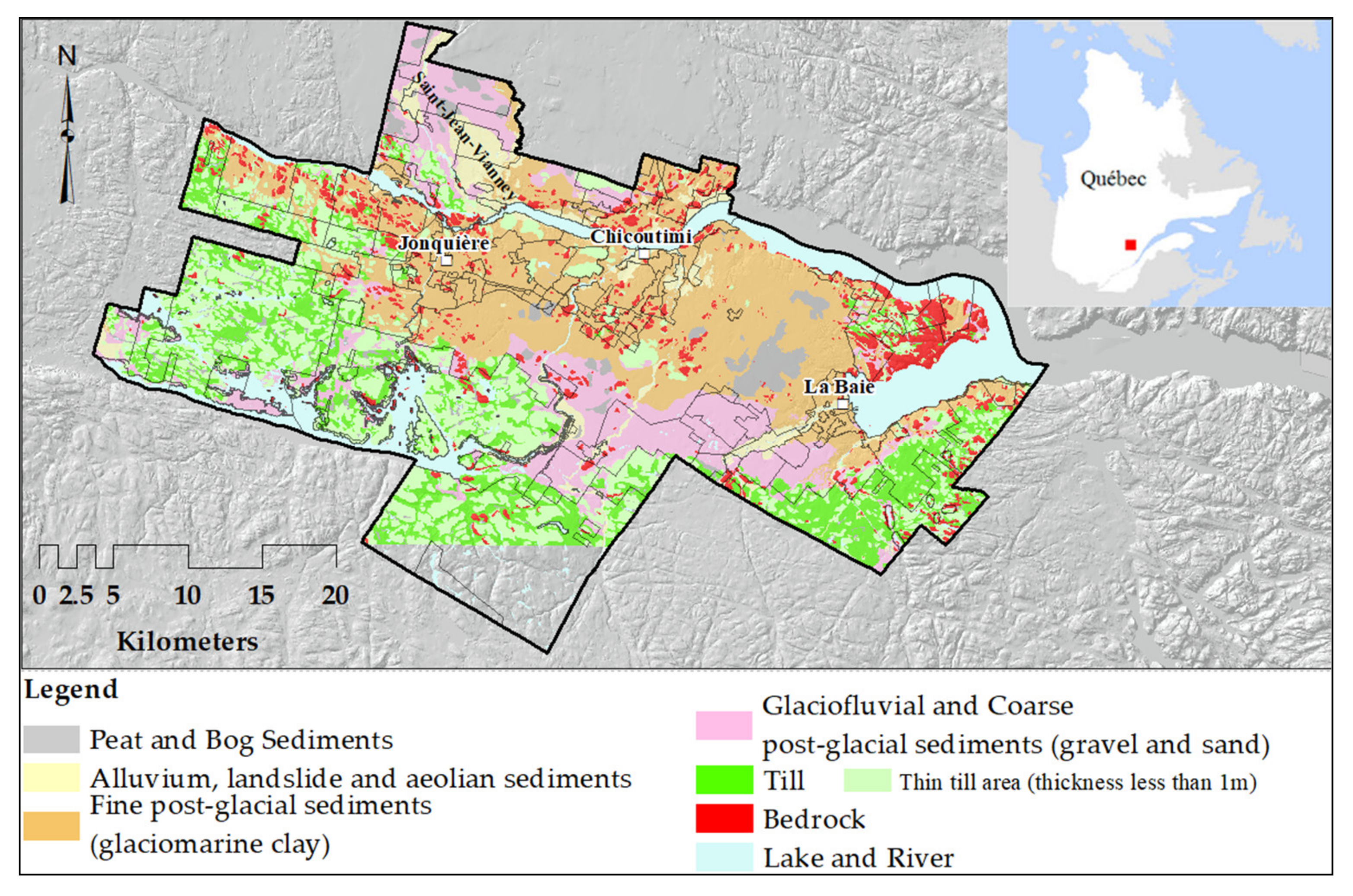
The bedrock of the Saguenay region is part of the Grenville Province of the Canadian Shield and is mainly composed of crystalline Precambrian rocks [31]. On the basis of the geological sections [32,33] and subsurface data [34], the soil deposits are grouped into two major geological classes: glacial and post-glacial sediments [35]. They can be further subdivided into five categories: till, gravel, clay, sand and other recent sediments (Figure 5).
  • Till: This glacial sediment is located at the base of the stratigraphic soil column; it is compact and semiconsolidated. Till is the most widespread soil unit in the study area and ranges in thickness from a few meters to >10 m at certain locations. In the highlands, the till veneer is frequently discontinuous and results in areas of rock outcrops. Most of the till outcrops are assumed to be less than 1 m thick on the geological map [33]. With the exception of rock outcrops, till continuously covers the bedrock elsewhere, representing an important assumption in the 3D modelling approach.
  • Gravel: This coarse sediment is mainly of glaciofluvial and alluvial origin; it consists of gravel, sand and sometimes till. This unit is occasional in the region, often in contact with till or sand units.
  • Clays: These fine post-glacial sediments are the most present soil type by volume in the study area. They are composed mainly of silt, silty clays and clay. They have a thickness of up to 10 m and may attain a maximum thickness of >100 m in the lowlands.
  • Sand: This group consists mainly of coarse glaciomarine deltaic and prodeltaic sediments and alluvial sands composed of sand and gravely sands.
  • Other sediments: This extremely heterogeneous category comprises all the remaining sediments; it mainly includes loose post-glacial sediments consisting of alluvium, floodplain sediments, organic sediments and occasional landslide colluvium that can be classified into sand, clay and gravel on the basis of grain size distribution.
The surficial deposit map in Figure 5 shows that till is the most widespread soil type at the surface, followed by clay and sand sediments.
Figure 5. Saguenay study area: surficial geology map (modified from Daigneault et al. [33]), [34].
Geosciences 11 00204 g005

4.2. Input Data and Analysis

Subsurface and surface data were collected from various sources of information (Figure 6). Borehole logs are the main subsurface data where the soil thickness data and soil types are obtained. The other invaluable sources of data are rock outcrops with zero soil thickness value; the virtual data derived from geological cross-sections and thin till data (thickness ≤ 1 m) interpreted from the surficial geological map. Borehole data were obtained from groundwater wells, exploration boreholes and geotechnical drilling logs. The brief descriptions of the input data stored in the database are as follows:
  • Borehole logs: The database contains 3524 borehole logs distributed over the study area [34]. A total of 2402 boreholes are sufficiently deep to reach the bedrock. The remaining 1122 boreholes that do not reach the bedrock indicate that the bedrock is deeper than the borehole depth, and a groundwater-bearing layer is possibly encountered in the coarse soil deposits.
  • Virtual logs: A total of 26 geological cross-sections distributed over the region were developed on the basis of expert opinion in previous geological studies [34]. These cross-sections include 973 virtual logs distributed in a regular spatial pattern at a distance of ~500 m to improve the data coverage mainly in the lowland areas (Figure 6).
  • Rock outcrops: During the geographic information system processing of the surficial geology map, additional 1033 data points were introduced to indicate rock outcrops. Located within the bedrock polygons, they improve the realistic spatial variability of the sediment thickness.
  • Till veneer: Till sediments cover most of the study area. Till outcropping areas, with a thickness equal to or less than 1.0 m, are located in the highlands and are referred to as a till veneer. In these areas, the till thickness is fixed to 1 m, and the till outcrop polygons are modelled with a mesh of 75 m, generating an additional 42,649 points with a known thickness.
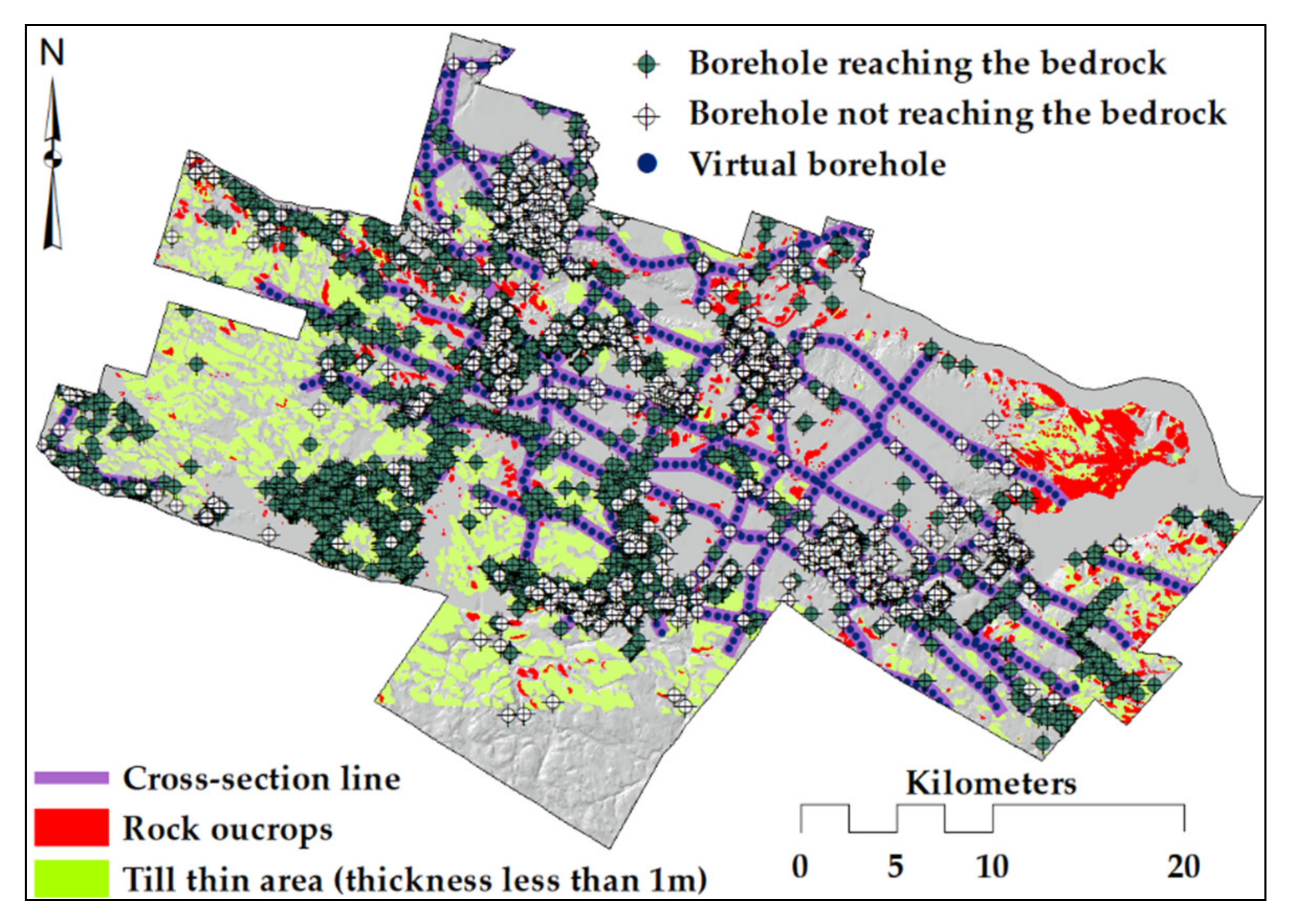
Figure 6. Complete set of the available observation points, including borehole logs, rock outcrops and shallow till data.
Geosciences 11 00204 g006
Rock outcrops (zero soil thickness) and shallow till data (1 m soil thickness) are valuable sources of complementary information, mainly in the highlands where they improve the accuracy of the geological model (Figure 6). However, the rock outcrops and till veneer points are observed over large areas of the region, in comparison with other data, which are limited to the borehole locations [36]. The resulting bias in the simulation of the soil types is avoided by using the rock and till outcrop data only to generate the bedrock and till topography maps and then excluding these later data for the simulation of other soil units. The till veneer data are only applied to create the thickness map of till deposits.
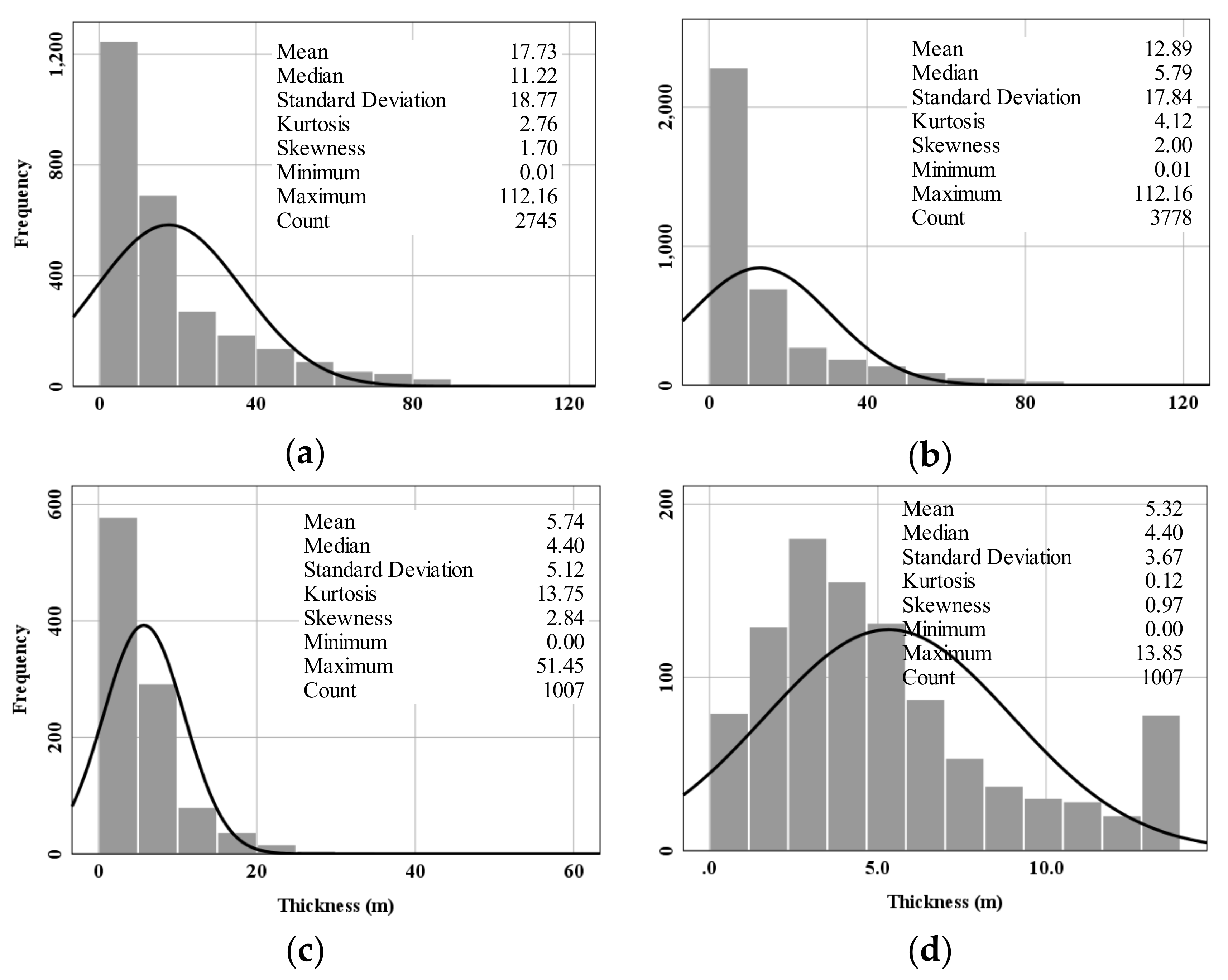
Figure 7 shows the histograms of the total soil thickness and thickness of glacial deposits. A total of 2745 soil thickness values are selected comprising the boreholes that reach the bedrock and virtual logs located in areas with sand, clay or gravel soil units. The average thickness of sediments over these areas is approximately 17 m with a positive skewness and a relatively high standard deviation of 18.7 m, indicating high thickness variability (Figure 7a). Important thicker parts are located in two areas: La Baie and Saint-Jean-Vianney (Figure 5). The incorporation of rock outcrops with zero soil thickness value decreases the average thickness (12.89 m), but the effects on the other parameters are minor (Figure 7b). A total of 1007 data points are selected from the virtual logs and boreholes reaching the bedrock at the location where the till sediments are exposed. Figure 7c illustrates that the average thickness of till is approximately 5 m in the borehole data, whilst the maximum nearly reaches 50 m. Attention must be given to the presence of outliers because they have a major influence on the interpolated surfaces [37]. Given that the expected thickness of till rarely exceeds 20 m, higher thickness values are most probably a consequence of poor logging of other soil units considered as outliers. The exact values of the outliers are determined using a box plot and are cases with values more than 1.5 times the interquartile range. Here, these values are replaced by a maximum of 13.85 m (Figure 7d). Following the replacement of the outliers of till thickness, the 1007 points are merged with till veneer and rock outcrop data in the database.
On the basis of the statistical summary, we can perceive existing high or low values, and the asymmetry of the probability distribution questions the stationarity. The asymmetry is evident in Figure 7 by comparing the observed thickness histograms and theoretical normal distributions of the different soil properties. In this context, traditional kriging methods (e.g., ordinary or transformed Gaussian kriging) do not perform well, whereas the EBK method is particularly helpful to overcome the nonstationarity by defining subsets (subareas) and automated variography analysis.
Table 1 provides the proportions of each soil unit based either on real or on virtual borehole logs. One of the main reasons for the differences in percentages is the clustered drilling pattern of the real boreholes drilled mainly in coarse sandy soils for drinking water supply. Given that virtual boreholes are designed in a systematic pattern, the percentages of virtual data are deemed reliable estimates for the layer thickness. The percentage values indicated in Table 1 denote the marginal probabilities that are applied in the geostatistical simulation using the Stanford Geostatistical Modelling Software [38].

4.3. Modelling Spatial Variation: Variogram Analysis

Two sets of directional variograms (not shown here) are calculated to determine the anisotropy axis and describe the spatial variation of soil types and their thickness. The first set uses a 2D coordinate system for the soil thicknesses, and the second set applies a 3D coordinate system for the soil types. Using the EBK method automates the fitting of variograms by simulating variograms per subset of data and then weighting the models using Bayes’ rule. The subsequent repetition of the process results in a spectrum of semivariograms rather than in a single one [39,40].
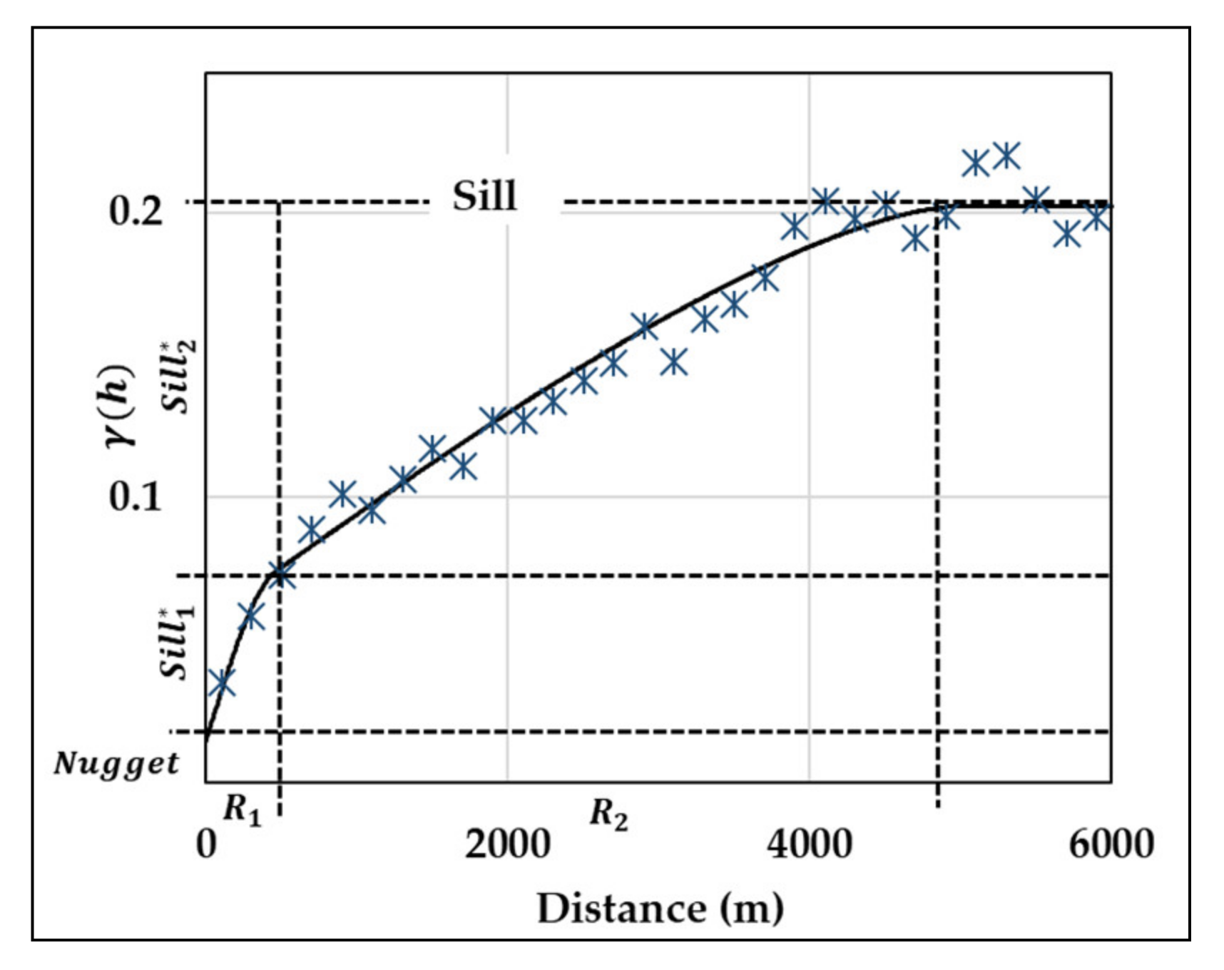
In the case of categorical variables, soil types, an indicator transformation is first performed. Indicator variograms are then computed to describe their spatial variability. The directional experimental variograms are computed using different lag sizes to capture the short- and long-scale variabilities. The experimental variograms show nested structures (e.g., Figure 8) and can be interpreted as a short- and a long-scale variability. The short-scale structure captures the variability over a distance of hundreds of meters and can be referred to as local soil variability. The long-scale structure captures the variability over a distance of thousands of meters and can be referred to as geological (stratigraphic) variability. In all the anisotropic models, the anisotropy is interpreted as geometric in which the range changes with the direction, whereas the sill is constant. Detailed discussion on variogram modelling can be found in [20].
Directional and omnidirectional variograms are analysed using a lag size of 25 m to model the variability at the short scale of all soil units. Lag sizes of 300 and 750 m are adopted to capture the variability at the long scale for gravel, sand and clay layers. The selected bandwidth is three times larger than the lag size to limit eventual deviation around the direction of the azimuth vector. The range of short-scale variability can be measured within hundreds of meters, as indicated in Table 2, whilst that of long-scale variability is within thousands of meters. Significant spatial variances are captured in short-scale variability, and the geometrical anisotropy with an azimuth angle of 135° corresponds to the geological continuity in the study area (Figure 5). As expected, the vertical range in all of the considered models is considerably lower than the horizontal ranges. The anisotropy consequently refers to the high density and the remarkable variation in data in the vertical direction compared with the horizontal.

5. Results

5.1. Construction of the Total Soil Thickness Map (Depth to Bedrock)

5.1.1. Spatial Interpolation

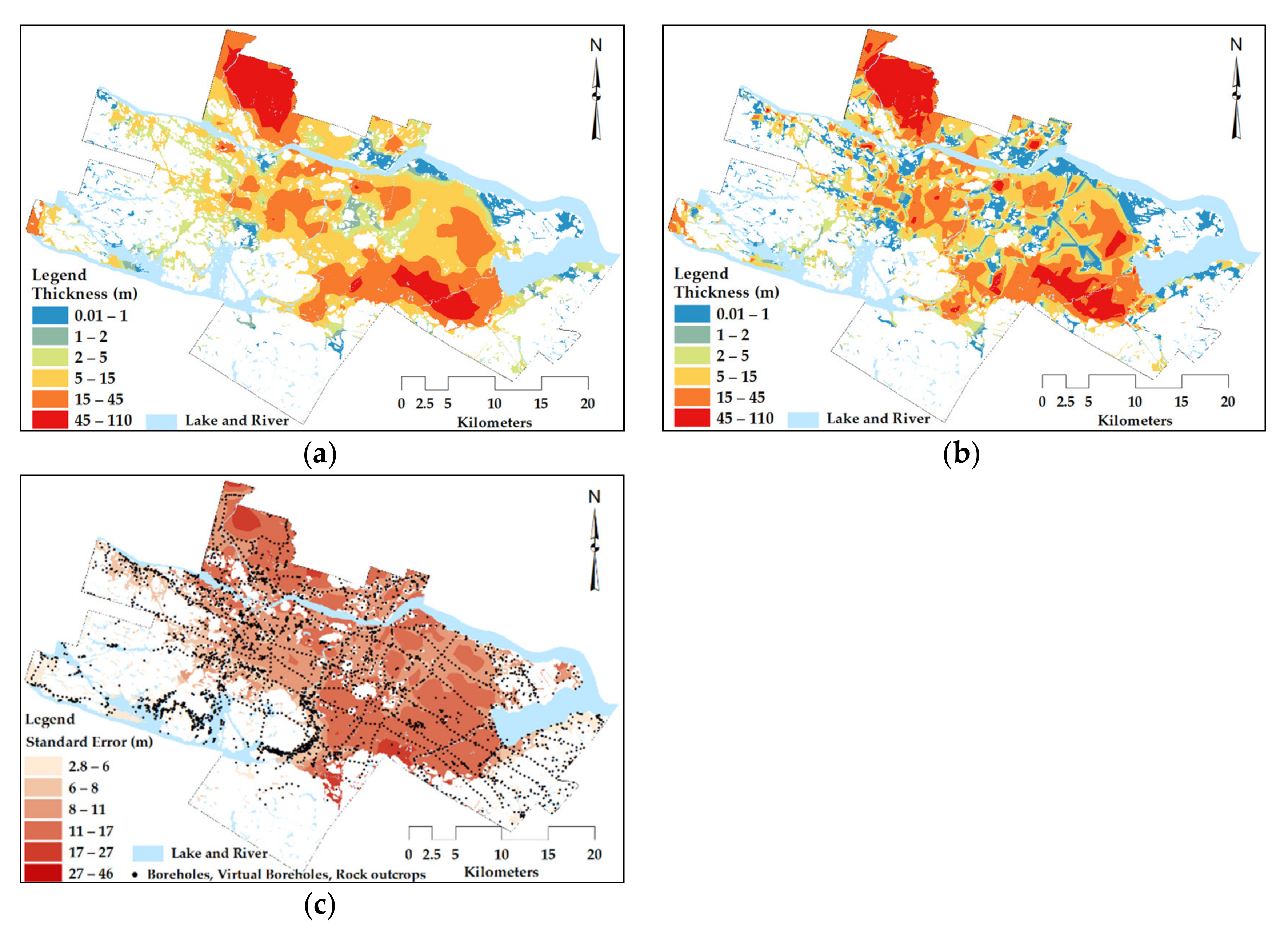
The spatial interpolation of the total soil thickness that represents the depth to bedrock map is performed by using the EBK method in addition to TIN. The study area is discretised into a regular grid of 902 × 637 cells with 75-m spacing. Figure 9a,b illustrate the resulting depth to bedrock maps. The estimated thickness of the deposits varies from zero to approximately 100 m, with similar variability patterns modelled by the two methods. The areas covered by till veneers and rock outcrops are excluded; they are indicated by the white background on the maps.
Figure 9c shows the spatial distribution of the standard deviation of the kriging with EBK ( σ ˜ k   ). As expected, lower uncertainties are associated with locations in the proximity of the existing data. However, relatively higher σ ˜ k   values are also observed, where the depth to rock is the highest. This phenomenon is a consequence of the locally varying mean and variance of the EBK method assumed as reliable results. TIN is a deterministic interpolation method and does not allow for the uncertainty of estimation.

5.1.2. Validation

Two approaches are applied to validate the estimation of soil thickness. The first approach is the routine cross-validation procedure in which the measured data are removed individually and re-estimated from the remaining dataset, referred to as the “leave-one-out method”. The second approach is based on a subset of data that is held back from the estimation process. In this case, the boreholes not reaching the bedrock are used as the validation dataset.
Cross-validation: The cross-validation procedure is used to optimise the estimation parameters. The optimised parameters include the lag size, the minimum and maximum numbers of participant data and the subset size in the EBK method. Four parameters are used to check the performance of the kriging methods: mean error (ME), root mean square error (RMSE), mean standardised error (MSE) and mean square standardised error (MSSE). The standardised values consider the kriging variance and are dimensionless. They provide an accurate comparison in addition to the statistical ME and RMSE values. The MSE values should be close to zero and can be obtained as follows (details can be found in [21]):
M S E = 1 N α = 1 n ( Z * u α Z u α σ ˜ k   u α ,
where N is the number of measured data, and Z * u α and Z u α   are the estimated and measured values of random variable Z at the location of u α , respectively. σ ˜ k   u α and σ ˜ k 2   u α are the kriging standard deviation and variance of the random variable Z, respectively.
The MSSE value should be close to one. For an MSSE greater than one, the variability in the estimated values is underestimated. Otherwise, the variability is overestimated. The parameter can be obtained with the following equation [21].
M S S E = 1 N α = 1 n ( Z * u α Z u α 2 σ ˜ k 2   u α .
Chiles and Delfiner [21] recommended a tolerance of 1 ± 3 2 N for the accepted MSSE. A total of 3778 measurements are used for estimating the total soil thickness in which the accepted tolerance is within the [0.93–1.07] range.
The cross-validation results reveal that (Table 3) the EBK method provides accurate and unbiased estimates with low ME and MSE values close to zero. The EBK method also gives relatively low values of RMSE and MSSE that vary within the acceptable tolerance range.
Validation using a test set: The 1122 boreholes that do not reach the bedrock, shown in Figure 6, were used as a test set for the soil thickness predictions. The depth of the observed point is underestimated when the total soil thickness estimates at these locations are lower than the observed borehole depths. Accordingly, the “thickness error” is considered the difference between the measured and estimated thicknesses, and only the positive errors are considered. Table 4 provides the statistical results of the thickness errors with respect to the different interpolation methods. The EBK method yields a lower number of underestimated soil thickness values at 313 boreholes, suggesting that this method provides better overall spatial predictions. When the mean error values and the sum of the errors are compared, EBK appears to provide slightly better predictions.
Figure 10 represents the distributions of the thickness error estimated by EBK in addition to the TIN methods. The thickness error is less than 10 m in approximately 60% of the underestimated borehole values. Overall, the results of the validation procedures indicate that the EBK method respects the observed values and provides accurate spatial predictions. This method provides a reliable measure of uncertainty at the estimation points.

5.2. Determination of the Till Thickness Map

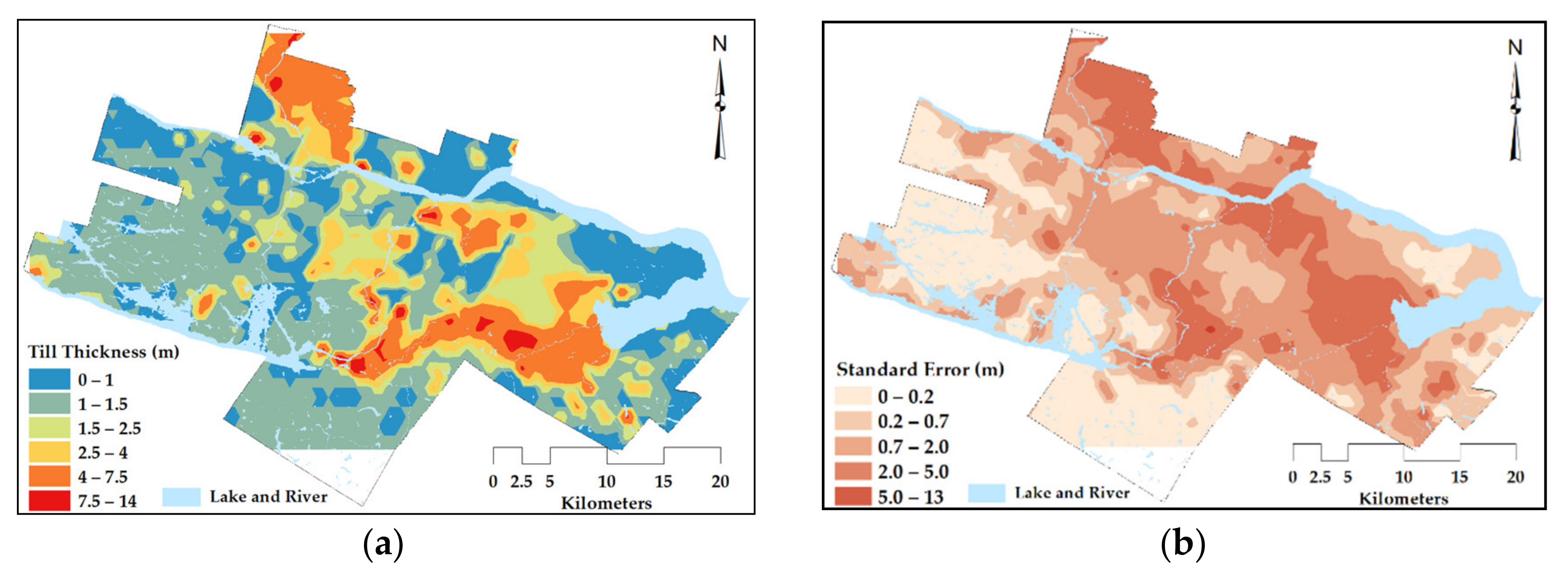
The spatial distribution of the till thickness as a continuous soil layer at the base of the Quaternary sequence is estimated with a similar procedure to the one applied for interpolation of the total soil thickness using the EBK method. The difference is that the outliers are replaced because the till deposits cannot be easily distinguished from the other soil types due to difficulties related to the presence of drilling mud. Thus, replacing the outliers of the till thickness data can be considered a conservative approach to estimate the thickness of other post-glacial deposits. Replacement is also an effective method for stabilising the variance. A complete set of observation points, including 2402 real and 973 virtual boreholes, 1033 rock outcrops and 42,649 points of thin till thickness (1 m), is incorporated to create the till thickness map. The thin thickness data dictate the highly skewed distribution of the 1 m data. Therefore, subsetting the data is a great advantage in using the EBK method. Figure 11 presents the resulting spatial distribution of the till thickness and the associated kriging standard deviation. Replacement of outliers combined with the use of shallow till data prevents potential soil thickness overestimation and generates conservative estimates for the future evaluation of the geotechnical soil parameters.

5.3. 3D Modelling of Discontinuous Soil Layers

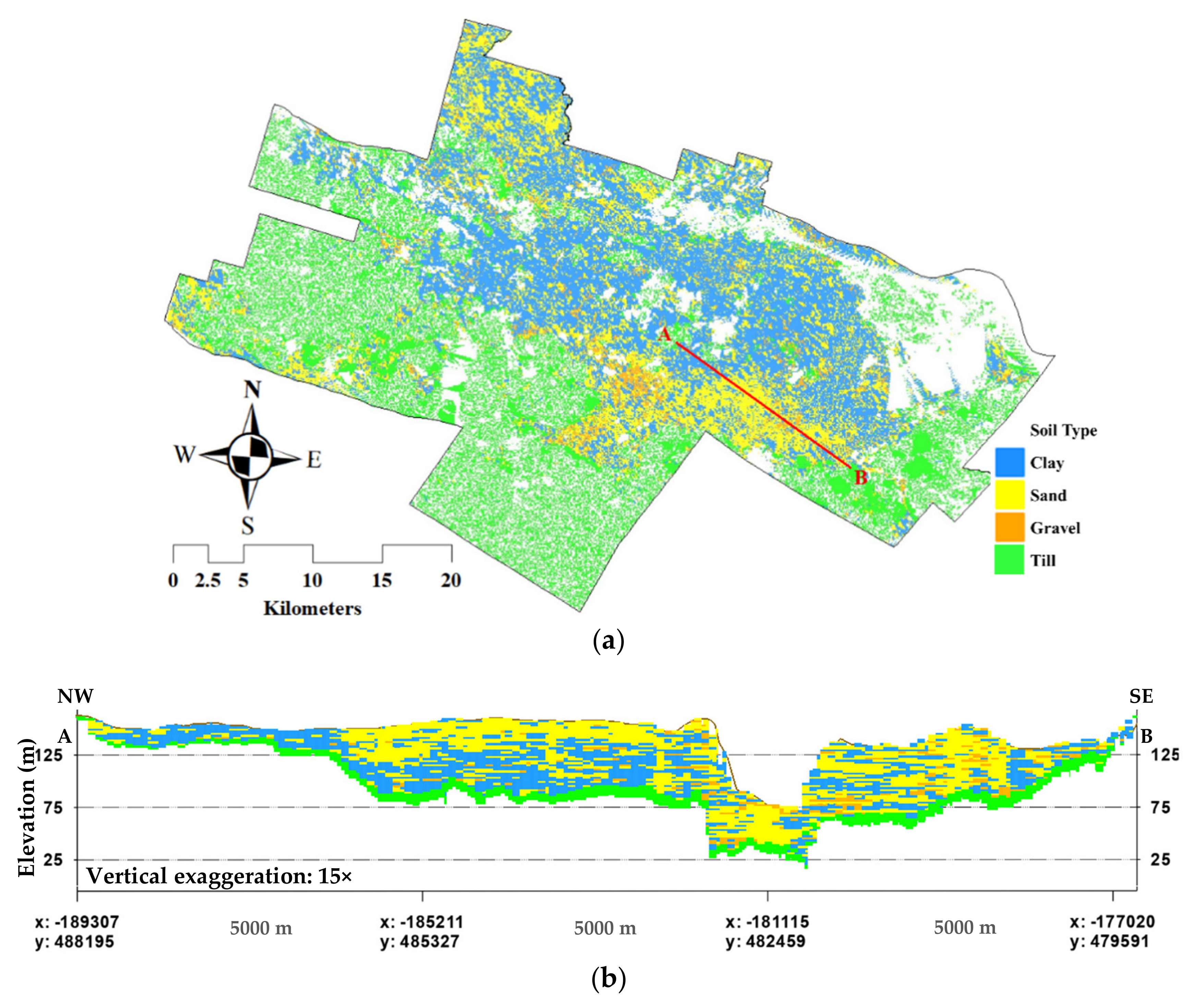
A full 3D volume is required to determine the soil type of discontinuous soil layers. The block model fills this volume, and each block represents the smallest unit of soil type using geostatistical simulation. For this purpose, the maps of bedrock and till topography are created by using digital elevation modelling, and total soil thickness and till thickness maps. When the bedrock and till topography maps are created, the space between the top and bottom of each surface is filled with 75 × 75 × 2 m blocks. Overall, 100 realisations are generated using the conditional SIS method to determine the probability of occurrence for each of the post-glacial deposits: clay, sand and gravel. Figure 12 shows a plan and cross-section through one of the SIS realisations in an area where all four surficial soil units are present.
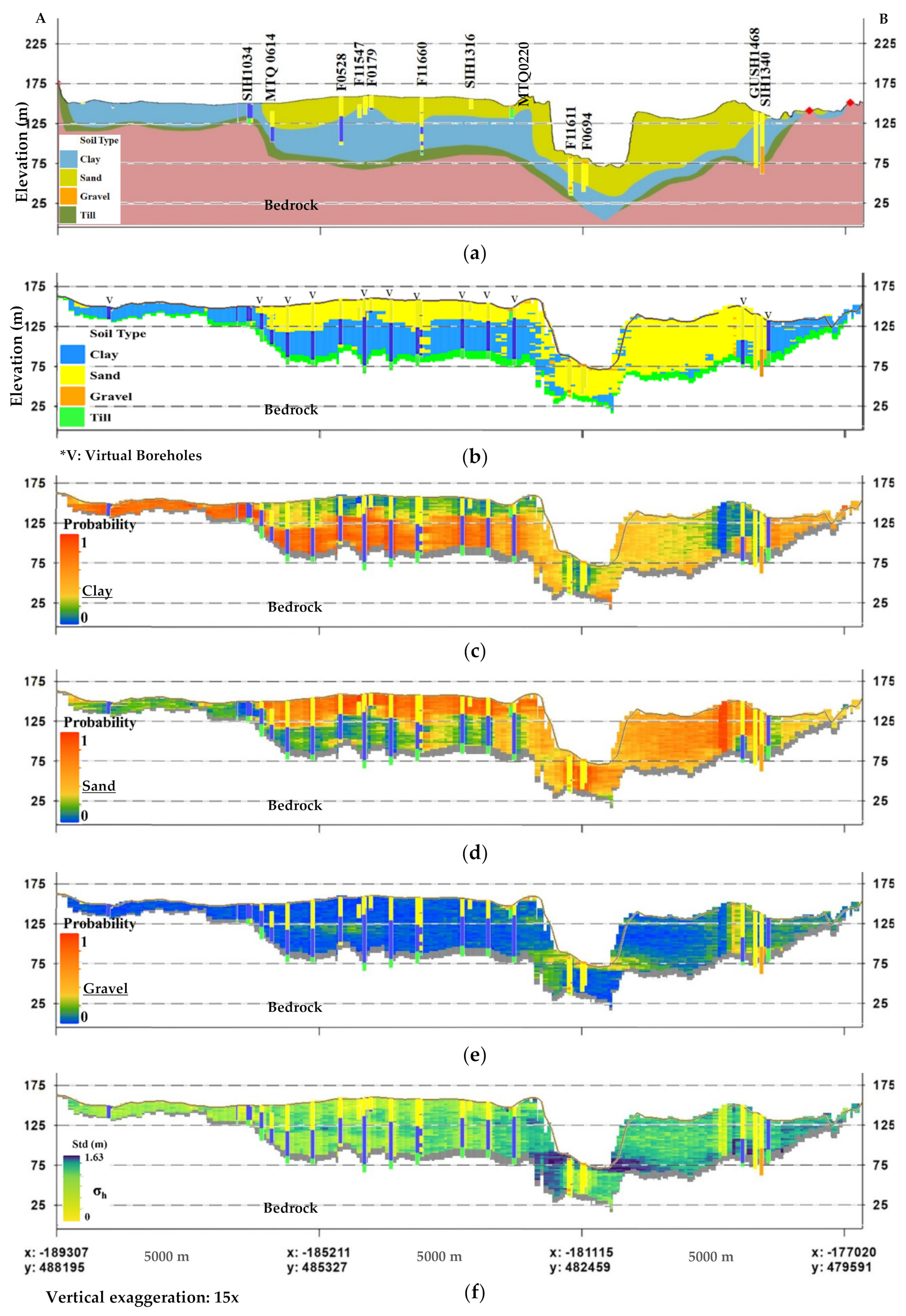
The results of the SIS simulation are visually compared with the deterministic geological cross-section (Figure 13). Figure 13a represents a part of the main cross-section of the study area (Figure 12a). Figure 13b shows the soil units with the highest probability of occurrence resulting from 100 realisations. The comparison of Figure 13a,b shows that the probabilistic model is consistent with the interpretations of expert geologists; however, it yields a realistic soil variability prediction corresponding to the real borehole data. This observation is particularly true when comparing the individual borehole logs or the entire right-hand portion of the cross-section extending from borehole F1161. This condition is mainly due to the nature of the probabilistic estimates that consider the entire set of input data and the extent of the geological units in 3D. Figure 13c–e present the probabilities of occurrence of the individual soil units. The 3D simulation of the discontinuous soil units quantifies the uncertainty of the predictions (Figure 13f) using the total standard deviation of the soil thickness computed from the probability of a categorical distribution for each block. The thickness standard deviation represents the total uncertainty that reaches its maximum in locations where the probabilities tend to be average, such as 0.5. The average probabilities are generated in two types of location: in the areas of contact between sand and clay or gravel and the areas with a high variability of soil types (locations near boreholes F11611 and SIH1340). This variability can be a result of errors in geological logging or from the inherent soil variability. The detailed computations of the thickness maps of post-glacial deposits and the associated uncertainty are discussed next.

5.4. Thickness Maps of Discontinuous Soil Layers

The above 3D probabilistic model provides the spatial distribution of the discontinuous soil units and their probability of occurrence within the regular 75 × 75 × 2 m blocks. In the determination of seismic parameters at a site (e.g., V s , 30 and T0), the geometry (soil thickness) and shear wave velocity ( V s i ) of each soil layer are important variables. Therefore, the 3D model must be transformed into a set of 2D thickness maps to obtain the thickness of the individual discontinuous soil units. Thus, the thickness mean and variance of each block are computed on the basis of the discrete probability distribution of the random categorical variable ( X i ) with an event probability p i as follows:
E X i = p i ,   V a r X i = p i 1 p i ,
where E X i is the mean, V a r X i is the variance and   x i     0 , 1 , i   1 , , k . The thickness mean and the variance are scaled at the 2 m height of the blocks, h, as follows:
E h X = h E X ,
V a r h X = h 2 V a r X .
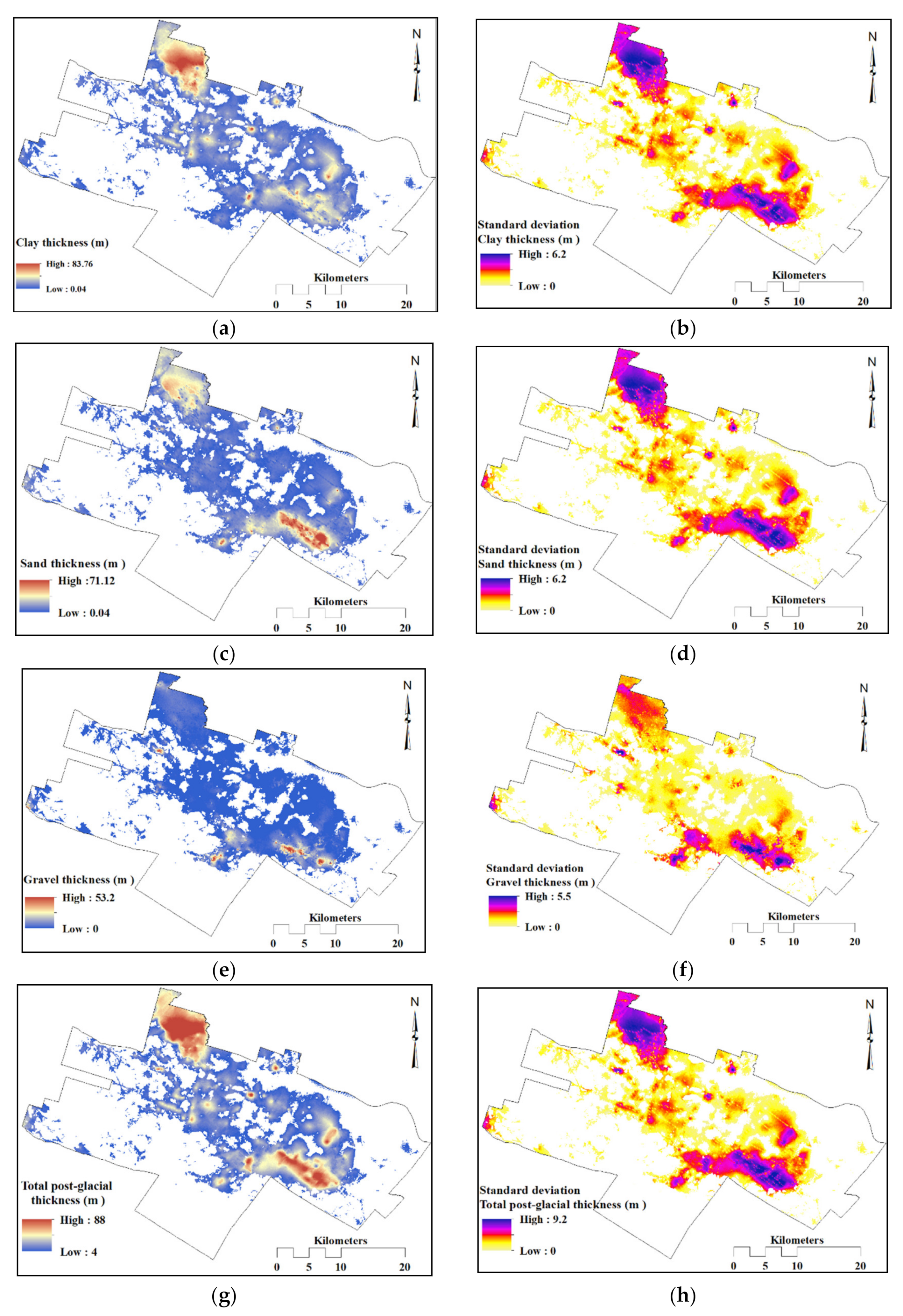
The thickness maps and the associated variances are obtained by computing the sum of the mean thickness and the variance of the blocks in a vertical column. In other words, the probabilities of occurrence are considered the weighting factors (Equation (8)) for the calculation of the soil thickness. In this case, the resulting thickness maps consider all the probabilities of occurrence for each soil type (not only the most probable one). The total variance for an individual soil unit (e.g., clay) is computed by summing up the block variance for each variable (Equation (9)) in a vertical column. The standard deviation is then computed as the square root of the total variance.
Figure 14 represents the weighted thickness maps based on the probability of discontinuous post-glacial deposits (clay, sand and gravel units) and the associated standard deviations of the thickness. A single pixel on these maps represents the weighted sum of the 2-m-high blocks in a vertical column for the same individual soil unit. The comparison of the standard deviation and thickness maps reveals that the local thickness uncertainty depends mainly on the following factors: differences between the presence of the discontinuous soil units in the neighbouring boreholes, the soil thickness values and the distances to the observation points. In other words, the greater the differences in the thickness or the distance, the greater the standard deviation.

6. Conclusions

This study adopted a combined multistep methodology of interpolation and simulation to develop a 3D geological model for geotechnical and seismic hazard evaluation at a regional scale. This approach focuses on considering geologic rules of stratification, reducing the effect of skewness of the observation points, and realistically predicting soil variability.
The interpolation procedure incorporates boreholes logs, in addition to the rock outcrop and shallow till data; these sources of data result in being invaluable in soil thickness mapping. Providing bedrock and till deposit maps allows considering the geologic rule of stratification of the basal till and the exclusion of low and zero thickness data from the simulation process of the discontinuous layers (i.e., clay, sand and gravel). The results of the validation and cross-validation verify that EBK is an appropriate interpolation method, producing an accurate outcome in regional studies involving extensive data with complexity.
SIS predicts the occurrence probability of discontinuous soil layers, as a representation of the soil type variability. The results indicate that the assumption of a continuous stratigraphic layer for the clay and for the sand and gravel units as drawn in the geological sections does not correspond to the real spatial variability of these layers. This observation is supported by the abrupt discontinuity and repetition of the deposits in the 3D model. The simulation of the soil type shows the benefit of considering the spatial soil variability and its associated uncertainty. The advantage is that the areas identified with increased uncertainty are characterised with considerable stratigraphic inconsistency and require further field measurements.
The proposed approach provides the basis for developing a reliable 3D shear wave velocity model including its uncertainties. The 3D geological and velocity models can enhance the mapping of seismic site parameters (e.g., V s , 30 and T0), which are important factors in seismic hazard assessment.

Author Contributions

Funding acquisition, A.S.; Methodology, M.S. and A.S.; Project administration, A.S.; Software, M.S.; Supervision, A.S., A.R. and M.N.; Writing—original draft, M.S.; Review & editing, A.S., A.R. and M.N. All authors have read and agreed to the published version of the manuscript.

Funding

This research was partially funded by the Natural Sciences and Engineering Research Council of Canada (NSERC) and Hydro-Quebec under project funding no. RDCPJ 521771–17.

Acknowledgments

The authors would like to thank the members of the CERM-PACES project for their cooperation and for providing access to the database.

Conflicts of Interest

The authors declare no conflict of interest.

Nomenclature

C ˜ 00  Variance of point values
C ˜ i j  Covariance between measured samples
C ˜ i 0  Covariance between measured and unknown values
EBK Empirical Bayesian Kriging
fo Fundamental site frequency of vibration
i u α ; k  Binary indicator value at location u α   and for category k
ME  Mean error
MSE  Mean standardised error
MSSE  Mean square standardised error
RMSE  Root mean square error
SIS Sequential indicator simulation
TIN Triangulated irregular network
To Fundamental site period of vibration
u Coordinates vector
V s  Shear wave velocity
V s , 30  Average shear wave velocity of the top 30 m
V S ,   a v g  Average shear wave velocity of the entire soil deposit
w i w j  Kriging weights
Z( u α ) Random variable at location u α
γ ^ h  Experimental variogram
γ ^ I h ; k  Indicator variogram for category k
σ ˜ k 2  Error variance of kriging

References

  1. Elkateb, T.; Chalaturnyk, R.; Robertson, P.K. An overview of soil heterogeneity: Quantification and implications on geotechnical field problems. Can. Geotech. J. 2003, 40, 1–15. [Google Scholar] [CrossRef]
  2. Fenton, G.A. Estimation for Stochastic Soil Models. J. Geotech. Geoenviron. Eng. 1999, 125, 470–485. [Google Scholar] [CrossRef]
  3. Phoon, K.-K.; Kulhawy, F.H. Characterization of geotechnical variability. Can. Geotech. J. 1999, 36, 612–624. [Google Scholar] [CrossRef]
  4. Fenton, G.A.; Griffiths, D.V. Bearing-capacity prediction of spatially random c–ϕ soils. Can. Geotech. J. 2003, 40, 54–65. [Google Scholar] [CrossRef]
  5. Uzielli, M.; Vannucchi, G.; Phoon, K.K. Random field characterisation of stress-nomalised cone penetration testing parameters. Géotechnique 2005, 55, 3–20. [Google Scholar] [CrossRef]
  6. Wang, Y.; Zhao, T.; Phoon, K.-K. Direct simulation of random field samples from sparsely measured geotechnical data with consideration of uncertainty in interpretation. Can. Geotech. J. 2018, 55, 862–880. [Google Scholar] [CrossRef]
  7. Zhao, T.; Wang, Y. Non-parametric simulation of non-stationary non-gaussian 3D random field samples directly from sparse measurements using signal decomposition and Markov Chain Monte Carlo (MCMC) simulation. Reliab. Eng. Syst. Saf. 2020, 203, 107087. [Google Scholar] [CrossRef]
  8. Ferrari, F.; Apuani, T.; Giani, G. Rock Mass Rating spatial estimation by geostatistical analysis. Int. J. Rock Mech. Min. Sci. 2014, 70, 162–176. [Google Scholar] [CrossRef] [Green Version]
  9. Pinheiro, M.; Vallejos, J.; Miranda, T.; Emery, X. Geostatistical simulation to map the spatial heterogeneity of geomechanical parameters: A case study with rock mass rating. Eng. Geol. 2016, 205, 93–103. [Google Scholar] [CrossRef]
  10. Kring, K.; Chatterjee, S. Uncertainty quantification of structural and geotechnical parameter by geostatistical simulations applied to a stability analysis case study with limited exploration data. Int. J. Rock Mech. Min. Sci. 2020, 125, 104157. [Google Scholar] [CrossRef]
  11. Vessia, G.; Di Curzio, D.; Castrignanò, A. Modeling 3D soil lithotypes variability through geostatistical data fusion of CPT parameters. Sci. Total. Environ. 2020, 698, 134340. [Google Scholar] [CrossRef]
  12. Lee, R.L.; Bradley, B.A.; Ghisetti, F.C.; Thomson, E.M. Development of a 3D Velocity Model of the Canterbury, New Zealand, Region for Broadband Ground-Motion Simulation. Bull. Seism. Soc. Am. 2017, 107, 2131–2150. [Google Scholar] [CrossRef]
  13. Rohmer, O.; Bertrand, E.; Mercerat, E.; Régnier, J.; Pernoud, M.; Langlaude, P.; Alvarez, M. Combining borehole log-stratigraphies and ambient vibration data to build a 3D Model of the Lower Var Valley, Nice (France). Eng. Geol. 2020, 270, 105588. [Google Scholar] [CrossRef]
  14. Hallal, M.M.; Cox, B.R. An H/V geostatistical approach for building pseudo-3D Vs models to account for spatial variability in ground response analyses Part I: Model development. Earthq. Spectra 2021. [Google Scholar] [CrossRef]
  15. Rosset, P.; Bour-Belvaux, M.; Chouinard, L. Microzonation models for Montreal with respect to VS30. Bull. Earthq. Eng. 2014, 13, 2225–2239. [Google Scholar] [CrossRef]
  16. Nastev, M.; Parent, M.; Ross, M.; Howlett, D.; Benoit, N. Geospatial modelling of shear-wave velocity and fundamental site period of Quaternary marine and glacial sediments in the Ottawa and St. Lawrence Valleys, Canada. Soil Dyn. Earthq. Eng. 2016, 85, 103–116. [Google Scholar] [CrossRef]
  17. Foulon, T.; Saeidi, A.; Chesnaux, R.; Nastev, M.; Rouleau, A. Spatial distribution of soil shear-wave velocity and the fundamental period of vibration—A case study of the Saguenay region, Canada. Georisk Assess. Manag. Risk Eng. Syst. Geohazards 2017, 12, 74–86. [Google Scholar] [CrossRef]
  18. Myers, D.E. Spatial interpolation: An overview. Geoderma 1994, 62, 17–28. [Google Scholar] [CrossRef]
  19. Li, J.; Heap, A.D. Spatial interpolation methods applied in the environmental sciences: A review. Environ. Model. Softw. 2014, 53, 173–189. [Google Scholar] [CrossRef]
  20. Isaaks, E.H.; Srivastava, M.R. Applied Geostatistics; Oxford University Press: New York, NY, USA, 1989. [Google Scholar]
  21. Chiles, J.-P.; Delfiner, P. Geostatistics: Modeling Spatial Uncertainty; John Wiley & Sons: Hoboken, NJ, USA, 2009; Volume 497. [Google Scholar]
  22. Krivoruchko, K.; Gribov, A. Evaluation of empirical Bayesian kriging. Spat. Stat. 2019, 32, 100368. [Google Scholar] [CrossRef]
  23. Mirzaei, R.; Sakizadeh, M. Comparison of interpolation methods for the estimation of groundwater contamination in Andimeshk-Shush Plain, Southwest of Iran. Environ. Sci. Pollut. Res. 2015, 23, 2758–2769. [Google Scholar] [CrossRef]
  24. Giustini, F.; Ciotoli, G.; Rinaldini, A.; Ruggiero, L.; Voltaggio, M. Mapping the geogenic radon potential and radon risk by using Empirical Bayesian Kriging regression: A case study from a volcanic area of central Italy. Sci. Total. Environ. 2019, 661, 449–464. [Google Scholar] [CrossRef]
  25. Chesnaux, R.; Lambert, M.; Walter, J.; Dugrain, V.; Rouleau, A.; Daigneault, R. A simplified geographical information systems (GIS)-based methodology for modeling the topography of bedrock: Illustration using the Canadian Shield. Appl. Geomat. 2017, 9, 61–78. [Google Scholar] [CrossRef]
  26. Goovaerts, P. Geostatistics in soil science: State-of-the-art and perspectives. Geoderma 1999, 89, 1–45. [Google Scholar] [CrossRef]
  27. Deutsch, C.V. A sequential indicator simulation program for categorical variables with point and block data: BlockSIS. Comput. Geosci. 2006, 32, 1669–1681. [Google Scholar] [CrossRef]
  28. Deutsch, C.V.; Journel, A.G. GSLIB Geostatistical Software Library and User’s Guide, 2nd ed.; Oxford University Press: New York, NY, USA, 1997; 369p. [Google Scholar]
  29. Du Berger, R.; Roy, D.W.; Lamontagne, M.; Woussen, G.; North, R.G.; Wetmiller, R.J. The Saguenay (Quebec) earthquake of November 25, 1988: Seismologic data and geologic setting. Tectonophysics 1991, 186, 59–74. [Google Scholar] [CrossRef]
  30. Lamontagne, M. An Overview of Some Significant Eastern Canadian Earthquakes and Their Impacts on the Geological Environment, Buildings and the Public. Nat. Hazards 2002, 26, 55–68. [Google Scholar] [CrossRef]
  31. Davidson, A. Geological Map of the Grenville Province: Canada and Adjacent Parts of the United States of America. Map 1947A; Geological Survey of Canada: Quebec City, QC, Canada, 1998. [Google Scholar]
  32. LaSalle, P.; Tremblay, G. Dépôts Meubles Saguenay Lac Saint-Jean. Rapport 191; Ministère des Richesses naturelles du Québec: Quebec City, QC, USA, 1978; 61p. [Google Scholar]
  33. Daigneault, R.-A.; Cousineau, P.; Leduc, E.; Beaudoin, G.; Millette, S.; Horth, N.; Allard, G. Rapport Final sur les Travaux de Cartographie des Formations Superficielles Réalisés dans le Territoire Municipalisé du Saguenay-Lac-Saint-Jean; Ministère des Ressources naturelles et de la Faune du Québec: Quebec City, QC, Canada, 2011. [Google Scholar]
  34. CERM-PACES. Résultat du Programme d’Acquisition de Connaissances sur les Eaux Souterraines de la Région Saguenay-Lac-Saint-Jean. Chicoutimi: Centre d’Études sur les Ressources Minérales, Université du Québec à Chicoutimi. 2013. Available online: http://paces.uqac.ca/programme.html (accessed on 29 April 2021).
  35. Walter, J.; Rouleau, A.; Chesnaux, R.; Lambert, M.; Daigneault, R. Characterization of general and singular features of major aquifer systems in the Saguenay-Lac-Saint-Jean region. Can. Water Resour. J. 2017, 43, 75–91. [Google Scholar] [CrossRef]
  36. Liang, M.; Marcotte, D.; Benoit, N. A comparison of approaches to include outcrop information in overburden thickness estimation. Stoch. Environ. Res. Risk Assess. 2013, 28, 1733–1741. [Google Scholar] [CrossRef]
  37. Wu, C.; Wu, J.; Luo, Y.; Zhang, H.; Teng, Y.; DeGloria, S.D. Spatial interpolation of severely skewed data with several peak values by the approach integrating kriging and triangular irregular network interpolation. Environ. Earth Sci. 2011, 63, 1093–1103. [Google Scholar] [CrossRef]
  38. Remy, N.; Boucher, A.; Wu, J. Applied Geostatistics with SGeMS: A User’s Guide; Cambridge University Press: Cambridge, UK, 2009. [Google Scholar]
  39. Pilz, J.; Spöck, G. Why do we need and how should we implement Bayesian kriging methods. Stoch. Environ. Res. Risk Assess. 2007, 22, 621–632. [Google Scholar] [CrossRef]
  40. Krivoruchko, K. Empirical Bayesian Kriging; ESRI: Redlands, CA, USA, 2012; Available online: http://www.Esri.Com/News/Arcuser/1012/Empirical-Byesian-Kriging (accessed on 29 April 2021).
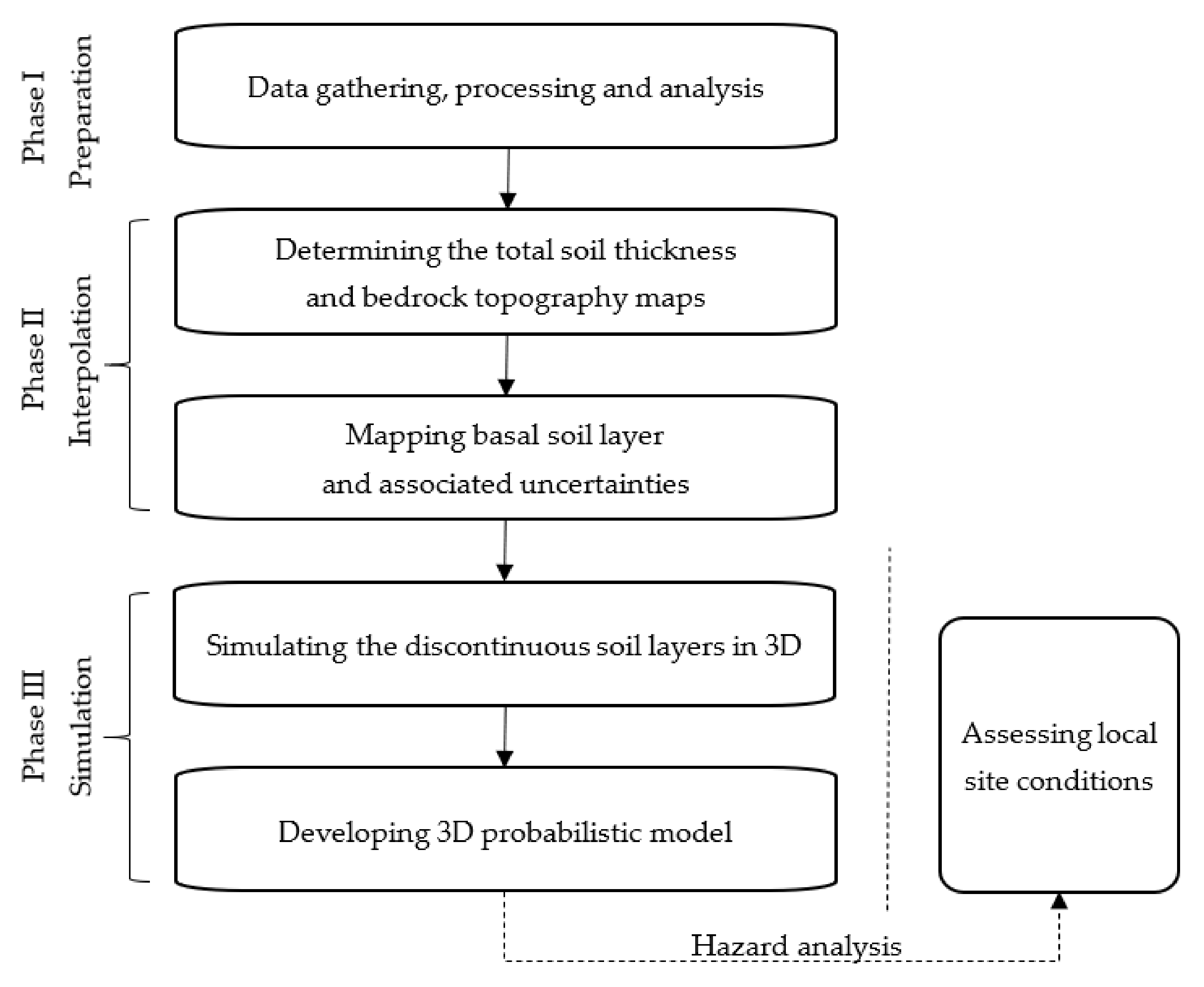
Figure 1. Methodology for developing a regional 3D probabilistic geological model.
Geosciences 11 00204 g001
Figure 2. Phase I: workflow of data preparation.
Geosciences 11 00204 g002
Figure 3. Phase II: workflow of the spatial interpolation of total soil thickness and thickness of the continuous basal layer.
Geosciences 11 00204 g003
Figure 4. Phase III: methodology for determining soil thickness map(s) and associated uncertainties of discontinuous soil layers using geostatistical simulation.
Geosciences 11 00204 g004
Figure 7. Thickness distributions of soil deposits as observed in borehole logs: (a) total soil thickness, depth to rock; (b) total soil thickness, including rock outcrops; (c) till sediments; (d) till sediments following replacement of outliers. The black line represents the normal distribution curve.
Geosciences 11 00204 g007
Figure 8. Example of variogram modelling: a nugget and two spherical nested structures are fitted on an experimental sample variogram. R1 and R2 refer to the ranges of the two nested models.
Geosciences 11 00204 g008
Figure 9. Total soil thickness maps obtained with: (a) EBK, (b) TIN; and (c) the map of the kriging standard deviation ( σ ˜ k   ) EBK. The areas with till or rock outcrops are excluded and indicated with white background.
Geosciences 11 00204 g009
Figure 10. Thickness error distributions for the test set of 1122 boreholes not reaching the bedrock estimated by (a) EBK and (b) TIN.
Geosciences 11 00204 g010
Figure 11. (a) Till thickness map and (b) kriging standard deviation,   σ ˜ k   .
Geosciences 11 00204 g011
Figure 12. (a) Plan and (b) cross-section of one SIS realisation of sand, clay and gravel. The thickness of the till unit shown in the cross-section is determined in Section 5.2.
Geosciences 11 00204 g012
Figure 13. Stratigraphic cross-sections: (a) deterministic based on expert opinion (modified from CERM-PACES [34]); (b) soil units with the highest probability of occurrence based on conditional SIS; individual probabilities of occurrence for (c) clay, (d) sand and (e) gravel obtained from a set of 100 conditional SIS; and (f) total standard deviation (σh) of the thickness computed by using the probability of categorical distribution.
Geosciences 11 00204 g013
Figure 14. Spatial distribution of the weighted thickness and associated spatial standard deviation (σh) for (a,b) clay, (c,d) sand, (e,f) gravel and (g,h) total post-glacial deposits.
Geosciences 11 00204 g014
Table 1. Percentage of each soil type based on real and virtual borehole logs.
Geological UnitReal Borehole Data (%) Virtual Logs (%)
Clay53.60%58.54%
Gravel6.80%2.06%
Sand35.66%18.37%
Till3.94%21.03%
Table 2. Variogram model parameters of the soil type indicators.
VariablesNumber of StructuresModel Properties
Structure 1
Model Properties
Structure 2
Model TypeAnisotropy Axis
(amax, amed, amin)
Model ParametersModel TypeAnisotropy Axis
(amax, amed, amin)
Model Parameters
Clay2Sp.(135°,45°,90°)Nugget: 0.01
R1: (375,212.5,75)
Sill1 *: 0.18
Ex.(135°,45°,90°)R2: (12825,4275,75)
Sill2 *: 0.05
Sand2Sp.(135°,45°,90°)Nugget: 0.02
R1: (412.5187.5,62.5)
Sill1 *: 0.17
Sp.(0°,0°,90°)R2: (12375,12375,62.5)
Sill2 *: 0.03
Gravel2Sp.-Nugget: 0.01
R1: (150,150,150)
Sill1 *: 0.026
Ga.(0°,0°,90°)R2: (4600,4600,150)
Sill2 *: 0.015
* Partial sill, R: range (meter), Sp.: spherical, Ex.: exponential, Ga.: Gaussian. Amax, amed and amin refer to the azimuths of the three principal axes of the anisotropy.
Table 3. Cross-validation results for the total soil thickness estimates using EBK methods.
ME (m)RMSE (m)MSEMSSE
0.058.940.010.94
Table 4. Thickness error results at the locations of 1122 boreholes known not to reach the bedrock.
Thickness ErrorTINEBK
Mean (m)12.211.8
Sum (m)3889.83682.6
Error count (boreholes)318313
Publisher’s Note: MDPI stays neutral with regard to jurisdictional claims in published maps and institutional affiliations.