1. Introduction
Disturbing underground pore pressure by fluid injection or production may induce significant changes in stress and strain fields in a subsurface reservoir, which can then propagate to neighboring layers both down- and upwards and even to ground surface or seabed [
1]. Such a mechanical behavior can be well described by the poro-elasticity theory (e.g., [
2,
3]) and have been used for characterization and monitoring of subsurface geomechanical behavior in many different areas of engineering and geoscience (e.g., [
4,
5,
6]). The same mechanical behavior is relevant for understanding geomechanics related to geological CO
2 storage sites. In particular, the interferometric synthetic aperture radar (InSAR) data acquired at the In Salah CO
2 storage project in Algeria have been successfully applied to understand the pressure front evolution and hydraulic communication network in the subsurface during the whole period (around 7 years) of CO
2 injection (e.g., [
7,
8,
9,
10]). In addition, Hu et al. [
11] showed how the change in temperature and pressure may influence CO storage capacity, which is also one of the main parameters together with the geomechanical integrity in the context of CO
2 storage characterization and monitoring.
When relating surface deformation to the change in pore pressure, stress, and strain in the subsurface, we need a well-developed solution-frame that can calculate the quantitative dependency between the surface deformation and disturbed pore pressure under realistic geological environment e.g., heterogeneous stratigraphy, arbitrarily-distributed pressure anomaly. The Geertsma’s solution [
2] is well known to provide good insights (as a first-order approximation) on how ground deformation behaves, when a fluid is injected into or produced yet only from an isotropic homogeneous subsurface. In addition, the Geertsma’s solution is relevant only for a disk-shaped reservoir with a uniform pressure perturbation. Du and Olson [
12] extended the Geertsma’s solution by numerically integrating the nucleus of poro-elastic strain over a rectangular prism so that the spatial change of pore pressure can be taken into account, followed by superposing results from each rectangular prism. Fokker and Orlic [
13] presented an advanced semi-analytical solution that is based on a boundary element method and can consider a multi-layered visco-elastic subsurface. The semi-analytical solution can be faster than e.g., finite element approach, but is still rather slow compared to the analytical Geertsma’s solution. Tempone et al. [
14] extended the Geertsma’s solution a bit further by adding a rigid layer beneath a compacting reservoir, and also reported a correction to an error found in [
15]. Lately, Mehrabian and Abousleiman [
16] not only provided a good overview of the analytical solutions developed further to address the limitations of the Geertsma’s solution, but also presented a poro-elasticity framework that can simulate an isotropic layered-stratigraphy.
The current study makes further improvements in such a Geertsma type problem by deriving a more-generalized analytical solution that can consider any number of finite-thickness layers, each of which can have not only different but also anisotropic stiffnesses. These novelties are not found in any of the previous studies mentioned above. The analytical solution requires a numerical Hankel transform, whose accuracy and efficiency are also discussed. The accuracy of the analytical solution is validated in comparison with a finite element solution. Then, we discuss the importance of the heterogeneity in the layers through a set of synthetic models. In addition, we discuss the possibility of applying the analytical solution for a spatially-varying pressure anomaly, not only a single cylinder-shaped constant pressure. The approach is based on a linear superposition and should be efficient, since it avoids the numerical integration presented by Du and Olson [
12]. At the end, we apply the analytical solution to analyze a realistic synthetic surface heave data that is made based on the In Salah CO
2 storage site in Algeria.
2. Analytical Solution for Anisotropic Layered Subsurface
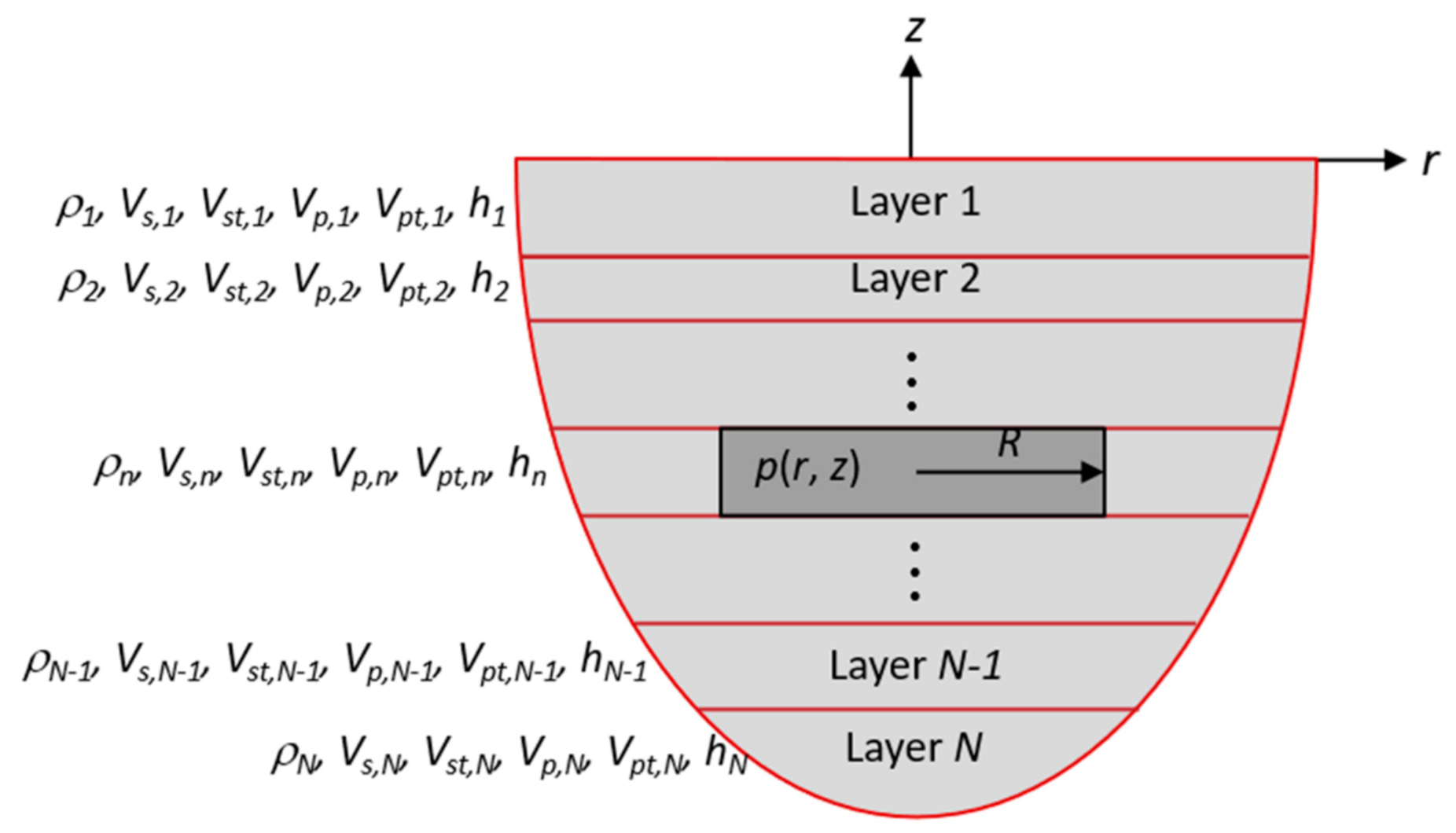
Here, we present an analytical solution for displacement field for an anisotropic layered subsurface subjected to fluid-induced pore pressure disturbance in a reservoir layer. The anisotropy herein refers to a particular case of vertically-transverse isotropic (VTI) stiffness, as shown in
Figure 1. Note that the anisotropy (horizontal-to-vertical velocity ratio) can be applied individually to S- and P-wave velocities and each layer may have different velocity ratios. The analytical solution is derived for a constant pressure change within a reservoir layer, and the pressure change is of cylinder shape i.e., axis-symmetric problem. The reservoir thickness can be any value, not only very small as in [
2]. In addition, any number of VTI or isotropic layers can be taken into account. Therefore, the analytical solution in the present study can be considered as a generalized Geertsma solution (GGS).
To derive the analytical solution for the VTI medium shown in
Figure 1, we apply the following axis-symmetric governing equation in cylindrical coordinate (
r,
z) and Hankel transforms with
k being the transform parameter (or wavenumber).
In the equations above,
ur and
uz are the radial and vertical displacements, respectively;
p is the pressure anomaly of radius
R; ∇ is the gradient operator; (
λ,
G) and (
λt,
Gt) are the two pairs of the
Lamé first parameter and shear modulus for the horizontal (or radial) and vertical directions, respectively;
α is the Biot coefficient. It is also noted that the
Lamé and shear moduli are related to the elastic P- and S-wave velocities as below by Park and Kaynia [
17]:
where
ρ,
Vs,
Vst,
Vp, and
Vpt are, respectively, mass density, radial/horizontal and vertical S-wave velocities, radial/horizontal and vertical P-wave velocities of each layer. Formally applying the Hankel transforms defined above to the governing equation, we obtain the governing equation in the
k-
z domain as below:
The solution to this linear system of ordinary differential equations can be obtained through a standard algebra and the final results are given below:
where:
In addition, there are four unknown coefficients of
A,
B,
C, and
D for each layer, which can be determined by satisfying the interface conditions between adjacent layers (i.e., displacement continuity and traction equilibrium). Furthermore, by imposing the zero-displacement boundary conditions at the bottom of the last finite-thickness layer, we can also simulate the rigid layer beneath a compacting reservoir studied by Tempone et al. [
14]. The related two traction components (
Srz and
Szz) at the layer interfaces can also be written in the
k-z domain as below:
Once we determine the four coefficients of A, B, C, and D for each layer, we can then obtain the final displacement field in the full-space (r, z) domain by performing numerically the Hankel transforms defined above. In theory, the integrations above should be done from 0 to infinite along parameter k. In practice, however, we should define the upper limit of parameter k (denoted as kmax) so that the numerical calculation can be terminated. Throughout an auxiliary numerical experiment, it is found that kmax is inversely proportional to the total thickness of the overburden (denoted as Hob), and the criterion of is suggested.
It is useful to notice that the horizontal S-wave velocity (
Vs) is not showing up in the final expression of the analytical solution. Therefore, if we know the vertical S-wave velocity (
Vst), we need to measure the anisotropic factor only for the P-wave velocity (
Vp,
Vpt). It is also important to remember that the solution derived above is valid only for VTI layers, not for an exact isotropic layer (i.e.,
Vp =
Vpt), because the linear independence among the four unknown coefficients are not valid for the exact isotropic case. For the latter, we need to use the corresponding solution for the isotropic medium, which is presented by Mehrabian and Abousleiman [
16]. Therefore, if both anisotropy and isotropy exist in a subsurface media, the two solutions are used jointly. Alternatively, to simulate an isotropic layer, we may specify the ratio of horizontal-to-vertical velocities as ~1 but not exactly 1.0, e.g., 1.001, which also produces almost the same result as that by the exact isotropic layer solution.
Correction to Mehrabian and Abousleiman
In addition to the analytical solution for the VTI medium derived above, we also write down the solution for the isotropic medium derived by Mehrabian and Abousleiman [
16], for the completeness of the current manuscript. It should also be noted that a few critical typos in Mehrabian and Abousleiman [
16] are found through [
18]. The corrected solutions for
U1,
U3,
Srz, and
Szz for the isotropic layer are given in the following form, using the two same parameters of
a and
cm as in [
16]:
where
,
(P modulus), and
ν is the Poisson’s ratio. Then, following the same Hankel transform procedure, we can calculate the displacement field for an isotropic layered subsurface subjected to the same type of axis-symmetric pore pressure disturbance of finite radius and thickness.
4. Representation of Arbitrarily-Distributed Pressure Anomaly
The analytical solutions presented above provide the surface deformations for a simple case where the pressure anomaly is uniform and cylindrical. However, the pressure in a real reservoir is typically non-uniformly and varies in space (
Figure 3a). In practice, such distribution can be described via a series of square-cuboid grids. Such a grid can be represented approximately by an equivalent cylinder (or drum) whose volume is the same as the square-cuboid grid (See
Figure 3b). Then, we can describe arbitrarily-distributed pressure anomaly of any shape by applying the linear superposition of the contribution from as many square-cuboid grids as needed, for each of which we apply the analytical solution presented in the current study and using the equivalent radius (
Req). The linear superposition can be expressed as below:
where
uz,i is the total vertical displacement at point
i,
gz,ij is a vertical displacement at point
i due to a unit-magnitude pressure anomaly at grid
j (i.e., so-called fundamental or Green’s function), and
pj is the pressure magnitude at grid
j. When we have the displacement at multiple points (
Figure 3a), then we can also write the linear superposition expression in the following matrix form:
with:
Note that the linear superposition expression in matrix form can also be used for an inversion problem where we invert known (or measured) surface displacement (Uz) to estimate pressure anomaly distribution (P). In this case, it is assumed that the subsurface model (layering and stiffness or the Green’s function matrix Gz) is known.
Figure 3.
(a) Schematic description of arbitrarily-distributed pressure anomaly. We assume that the pressure anomaly is discretized into J number of square-cuboid grids, to each of which a value of pressure pj is specified. The vertical displacement at a point (say uz,i) on the surface can be obtained by linearly summing up the contribution from all the pressure grids. (b) Illustration of an equivalent cylinder (radius Req = Lre/√π) to a square-cuboid of length Lre. Note both of the square-cuboid and the equivalent cylinder have the same height of Hre.
Since the equivalent-radius representation is an approximation, we need to know its performance and limitation so that we can decide
Req to be used without introducing any significant error in the calculation. To investigate this issue, we perform a parameter study by using FE simulation (COMSOL Multiphysics™, version 5.3.0.316). Namely, we compare two FE solutions obtained (1) by the exact square-cuboid shape pressure anomaly and (2) by the equivalent-radius cylinder shape pressure anomaly, respectively, with varying the lateral length of reservoir pressure anomaly (length,
Lre). For the simplicity in calculation, we simulate an isotropic homogeneous half-space of 1 GPa shear modulus and 0.25 Poisson’s ratio.
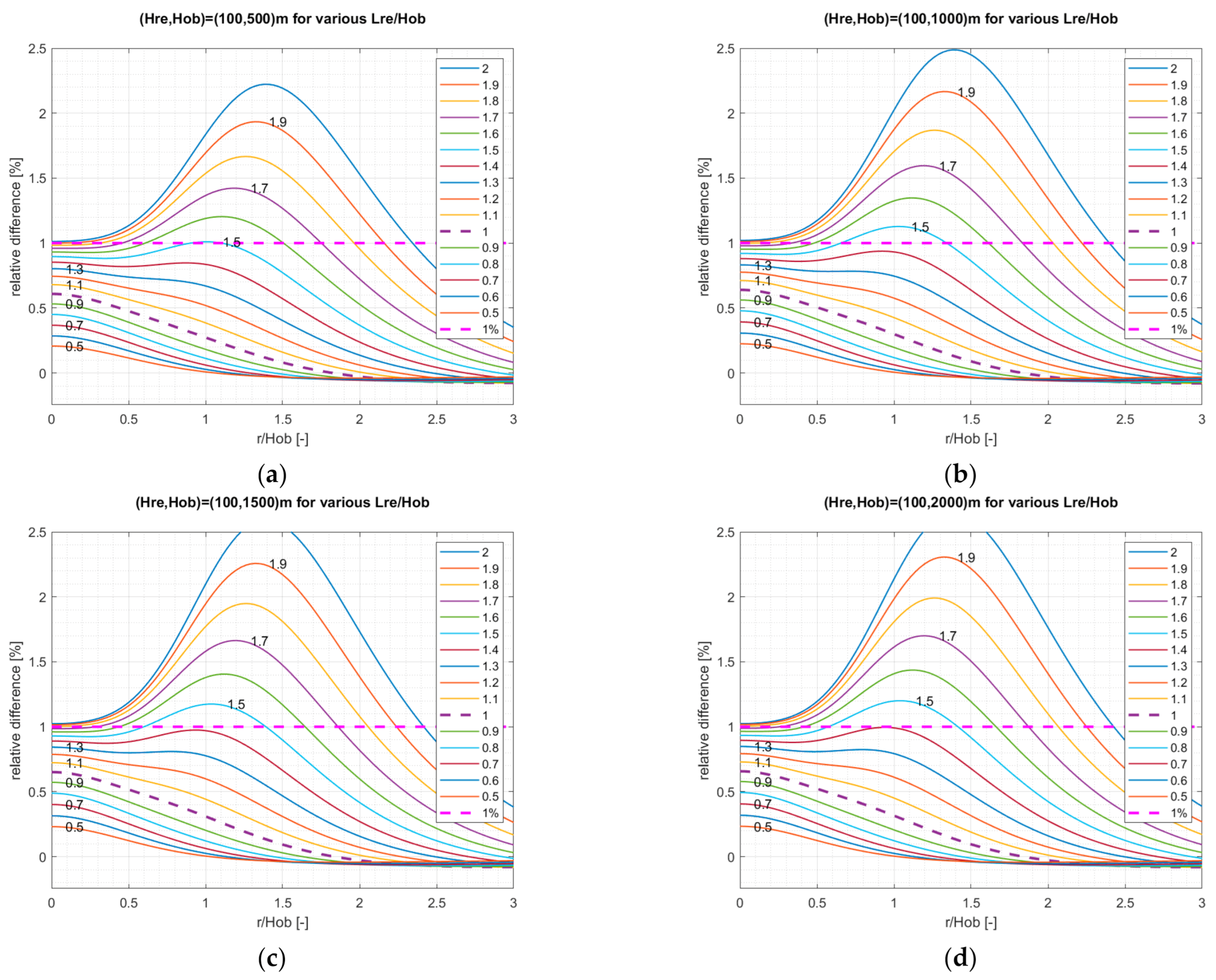
Figure 4 shows the results of the parameter study by plotting the relative difference between the two FE solutions versus the ratio of the radial coordinate to the overburden thickness (
Hob). Note that in the parameter study we fix the pressurized reservoir thickness (
Hre) to be 100 m, while we consider four different overburden thicknesses of 500 m, 1000 m, 1500 m, and 2000 m. In addition, for each overburden thickness, we vary the ratio of
Lre/
Hob from 0.5 to 2. As shown in
Figure 4, the relative difference between the two FE solutions depends on all the parameters used in the current sensitivity. It is also noticed that the dependency is most influenced by the ratio of
Lre/
Hob, and the cylinder-shape approximation for a square-cuboid-shape constant pressure anomaly works very well (<1% relative error) as long as
Lre/
Hob ≤ 1.4–1.5 (depending on reservoir depth). For the practical purpose, we choose the condition of
Lre/
Hob ≤ 1.0 (i.e.,
Req/
Hob ≤ 1/√π) in order to guarantee the accurate displacement calculation at the top surface for a square-cuboid shape pressure via the equivalent cylinder shape pressure. The purple dashed lines in
Figure 4 correspond to the upper limit of the criterion (i.e.,
Lre/
Hob = 1.0). However, note that the real size for
Lre (i.e., size of square-cuboid grids) to be used is also depending on the spatial variation of pore pressure disturbance in the subsurface e.g., sharp variation requiring smaller
Lre.
5. Synthetic Model Study Inspired by in Salah CO2 Storage Dataset
Here, we apply the linear superposition approach presented in the previous section to a realistic synthetic model and evaluate the performance by comparing with a full 3D FE solution. Furthermore, we also utilize the same superposition approach in the context of the simple inversion problem described earlier to explore the influence of the subsurface properties on the inverted pressure. For these purposes, we use an available FE model that was made for the history-matching study of the injection data and surface heave of the In Salah storage site [
3]. To make things simpler, we remove the vertical fault (F12) at Well KB502, and the pressure build-up within the fault from the FE simulation. Namely, we take only the pressure build-up in the reservoir layer of 20 m thickness from the FE simulation results, and produce a synthetic surface deformation data by means of the simplified FE model. Then, using the superposition approach combined with the analytical solution derived in the present study, we invert for the reservoir pressure.
Table 2 shows the layering and material properties for the In Salah model simplified from [
3]. In addition,
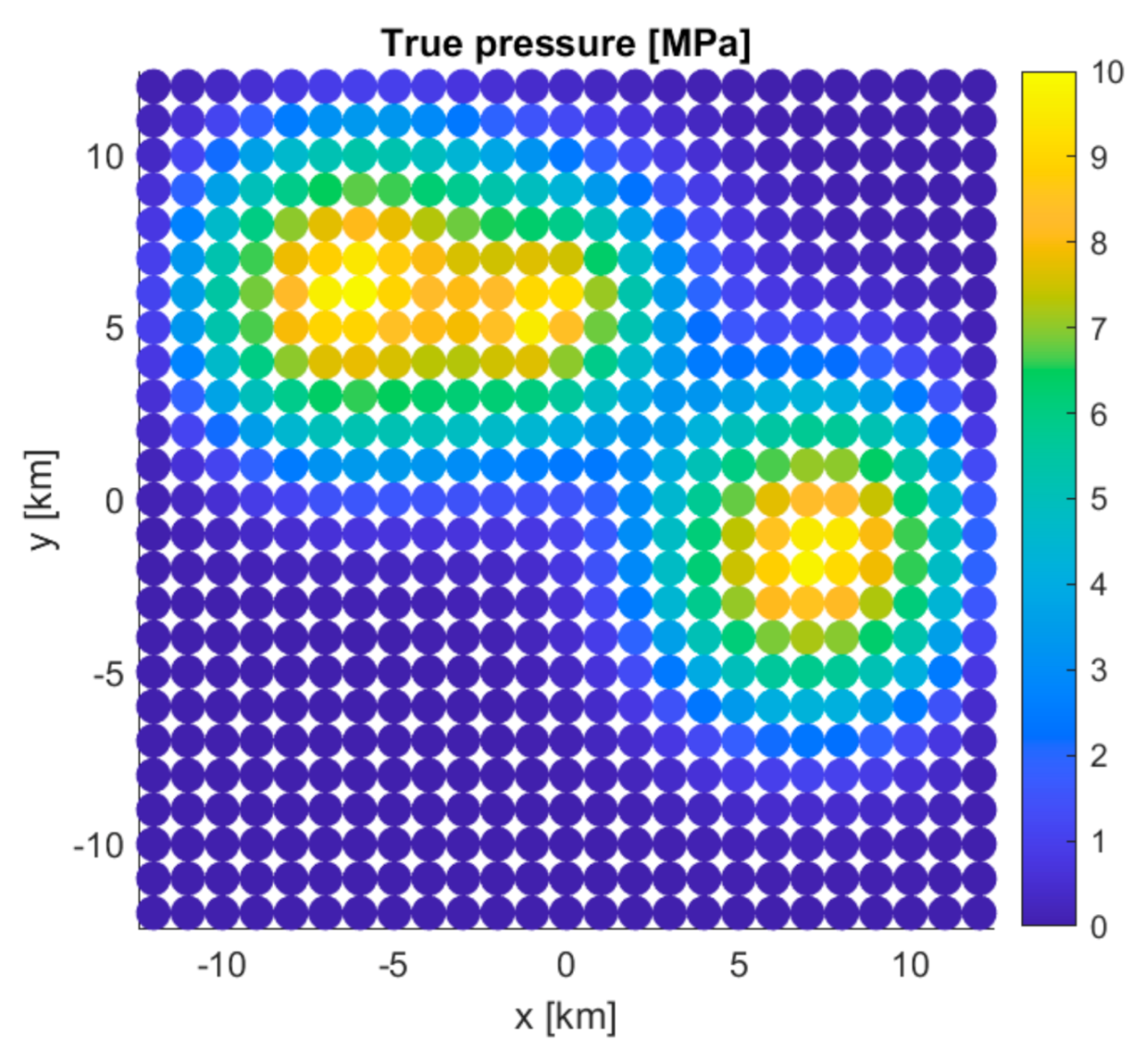
Figure 5 shows the reservoir pressure change calculated by Bjørnarå et al. [
3] in a grid setting of 1000 m × 1000 m × 20 m (i.e.,
Lre = 1 km and
Hre = 20 m for each square-cuboid grid), covering a large area of 25 km × 25 km.
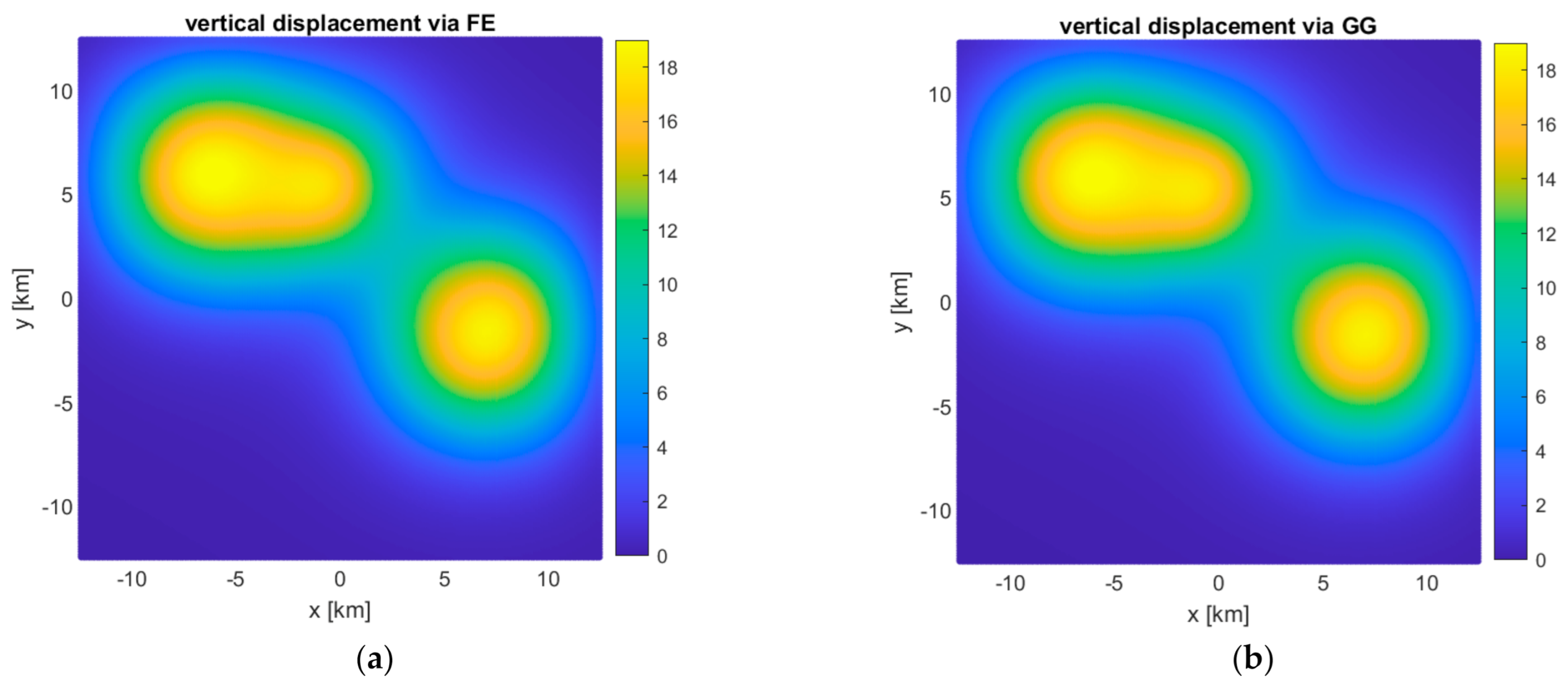
First, we re-calculate the surface deformation resulting from the reservoir pressure build-up shown in
Figure 5 yet now by using the linear superposition approach with the analytical solution derived earlier in order to check if the linear superposition approach produces the same results as the simplified FE model. The comparison of the results is shown in
Figure 6. It is clearly seen that the two results look almost identical to each other. Note that the surface deformation in
Figure 6 is plotted in a grid setting of 125 m × 125 m.
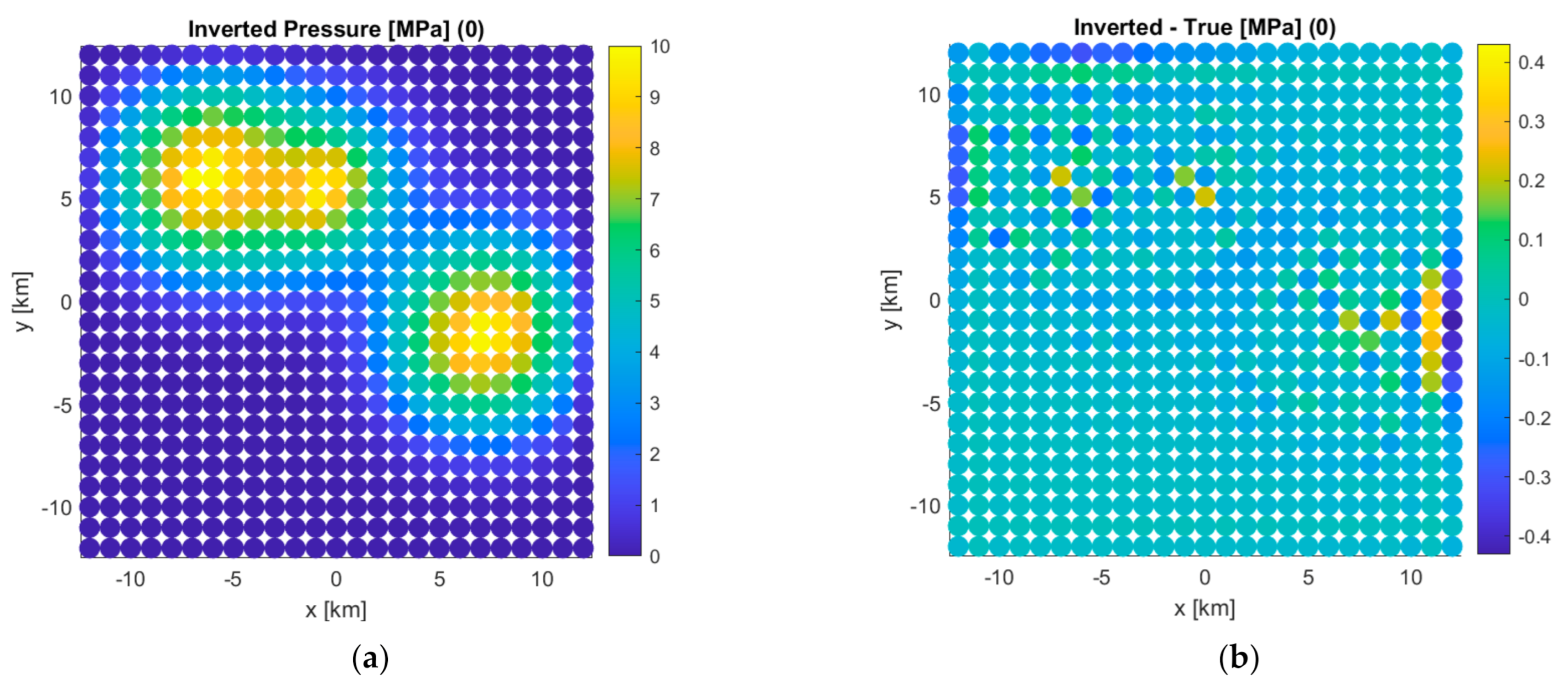
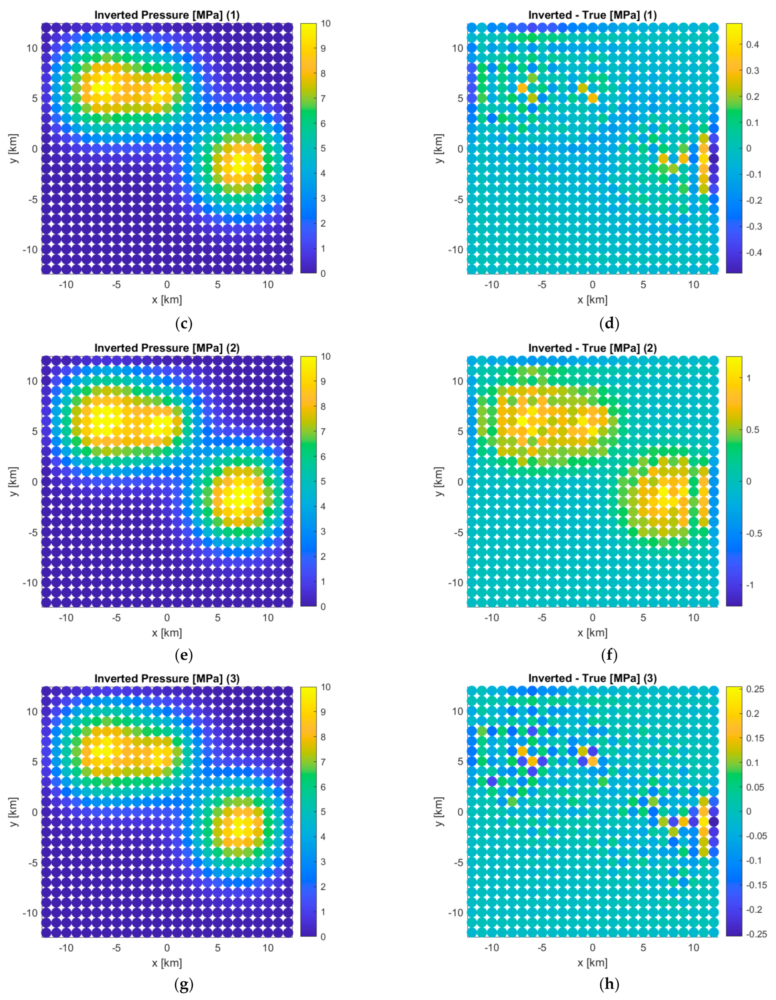
The next task is to invert the surface deformation calculated by the FE model (i.e., shown in
Figure 6a) by means of the inversion idea explained earlier. In our inversion study here, we introduce some changes in the layer stiffness to see the impact of such stiffness change on the inverted reservoir pressure build-up. Namely, we increase the stiffness of each layer by 10% in the three different following scenarios. In Scenario 1, we increase the stiffnesses of Layers 1–3, while keeping the other layers’ stiffnesses unchanged. In Scenario 2, we increase the stiffnesses of only Layers 4 and 5 and in Scenario 3, for Layer 6 only. In addition, we also run the inversion without changing any stiffness as Scenario 0. The inversion results for all the four scenarios are plotted in
Figure 7 in terms of inverted pressure (left panels) and difference between inverted and true (right panels). It is clearly shown that the stiffness change has noticeable impact on the inverted pressure, and the impact is the most significant (more than 1 MPa or 10%) when the stiffnesses of cap rock and reservoir are changed (Scenario 2 and shown in
Figure 7e,f). This observation illustrates that it is very important to estimate the high-confidence stiffnesses of cap rock and reservoir in comparison to the other layers in the subsurface.
6. Conclusions
We have presented a generalized Geertsma solution that can consider any number of layers in the subsurface whose properties and thicknesses can be different from layer to layer. In addition, each layer can be VTI anisotropic, with which more realistic stiffness can be simulated depending on condition of in situ stress or sediment bedding plane. The accuracy of the newly-derived analytical solution is validated with respect to an FE-based reference solution. Furthermore, it is found that the Hankel transform to be numerically performed can be done via a definite integral whose upper limit can be determined optimally as inversely proportional to the overburden thickness (i.e., ). The generalized Geertsma solution is then applied to a linear superposition framework via square-cuboid-shaped grids so that we can calculate arbitrarily-distributed pressure anomaly cases, not only the simple case of a constant pressure anomaly of cylinder shape. Furthermore, we have also defined the condition that the lateral length of a square-cuboid should be shorter than the overburden thickness (i.e., Lre/Hob ≤ 1.0) in order to guarantee the accurate displacement calculation at the top surface for a square-cuboid shape pressure via the equivalent cylinder shape pressure. The performance of this linear superposition approach is tested by solving a realistic synthetic model based on the In Salah CO2 storage site, simplified by removing the vertical fault in Well KB502. Finally, we look at the influence of subsurface stiffness on inverted pressure by means of a simple inversion based on the linear superposition approach. It is learned that the stiffnesses of cap rock and reservoir are the most influencing parameters on the inversion result, suggesting that it is very important to estimate the mechanical properties of cap rock and reservoir with high accuracy (i.e., low uncertainty).
The next step to follow up among many possibilities would be that we apply the solution approach presented in the current study to real data inversion of the In Salah storage with taking into account known fault structure such as F12. For this purpose, we may have to improve a limitation of the current approach that the subsurface should be a horizontally-layered medium and cannot consider any tilted structure (e.g., faults with different properties from layers). Tackling this limitation is our immediate task to pursue. Finally, since the analytical solution approach is fast, its application to machine learning-based inversion is also a desired task to follow up.


