Abstract
Structural geological models are widely used to represent relevant geological interfaces and property distributions in the subsurface. Considering the inherent uncertainty of these models, the non-uniqueness of geophysical inverse problems, and the growing availability of data, there is a need for methods that integrate different types of data consistently and consider the uncertainties quantitatively. Probabilistic inference provides a suitable tool for this purpose. Using a Bayesian framework, geological modeling can be considered as an integral part of the inversion and thereby naturally constrain geophysical inversion procedures. This integration prevents geologically unrealistic results and provides the opportunity to include geological and geophysical information in the inversion. This information can be from different sources and is added to the framework through likelihood functions. We applied this methodology to the structurally complex Kevitsa deposit in Finland. We started with an interpretation-based 3D geological model and defined the uncertainties in our geological model through probability density functions. Airborne magnetic data and geological interpretations of borehole data were used to define geophysical and geological likelihoods, respectively. The geophysical data were linked to the uncertain structural parameters through the rock properties. The result of the inverse problem was an ensemble of realized models. These structural models and their uncertainties are visualized using information entropy, which allows for quantitative analysis. Our results show that with our methodology, we can use well-defined likelihood functions to add meaningful information to our initial model without requiring a computationally-heavy full grid inversion, discrepancies between model and data are spotted more easily, and the complementary strength of different types of data can be integrated into one framework.
1. Introduction
In geophysical applications, inversions are popular tools to find properties within media that we cannot access through direct observations. Often, data-driven approaches are used where the subsurface is divided into grid cells to which petrophysical properties are assigned. Especially in cases where a regular Cartesian grid is used for this discretization step, the cell boundaries are not necessarily conforming to the geological contacts, but rather are artifacts of the grid [1,2,3]. To avoid geologically unrealistic outcomes and to omit the influence of the gridding, geophysical inversion can be naturally constrained by surface-based modeling, where a rock property is assigned to a surface. By considering the structural geological model as part of the inference, rock property and subsurface geometry can be integrated. This integration is essential to understanding mineral systems, where there is a complex interaction of different physical processes. It is known that geological structure plays an important role in this (e.g., [4,5,6]) and ideally geological, geophysical and geochemical data would have to be considered together. Data integration, though not straightforward in its implementation, becomes increasingly relevant as data acquisition is getting cheaper and faster, and often large amounts of different types of data are available. Additionally, despite the abundance of data and advances in increasingly sophisticated geological modeling methods and geophysical inversion practices [7], another limitation of common geoscience analysis remains too: the resulting model is often only one possible representation of reality, and uncertainties are often inadequately handled.
A Bayesian viewpoint provides a way forward to address these issues [8,9]. In this viewpoint, all information is expressed in the form of probabilities, representing a state of information. New information on any type of data can be incorporated into the inversion framework using likelihood functions. Likelihood functions provide a quantification of the likelihood of the model parameters in the light of the observed data. Probabilistic inference is used in different fields to analyze complex systems with incomplete data, and within geosciences particularly gained ground in the field of geophysics since the pioneering works of Tarantola and Valette [10], Mosegaard and Tarantola [11], and Sambridge and Mosegaard [12]. Probabilistic inference in practice often relies on Markov chain Monte Carlo (MCMC) algorithms to approximate the solution numerically [8,9]. In complex problems, this process can become computationally costly. Fortunately, MCMC is used in many different fields and the algorithms are getting increasingly sophisticated. Recent developments of gradient-based algorithms [13] provide solutions for efficient computation of higher dimensional problems.
Probabilistic inference inherently provides an uncertainty quantification as the solution consists of an ensemble of models that all fit the data to a certain degree. This allows us to consider inherent uncertainty in geological models and to use this information to constrain the inverse problem and to address problems of incompleteness and noisiness of geophysical data. The consideration of uncertainties in structural geological models has been getting increasing attention [7,14,15,16,17] and applications to mineral systems have shown relevance in both analysis and visualization [18,19,20]. There are promising results for the integration of additional information to the geological model through the implementation of a Bayesian modeling framework from synthetic studies [17,21], as well as application to a mineral setting [22]. In this paper, we present a similar Bayesian modeling framework for geological modeling, where we combine geophysical and geological data. The novelty of this work is that we consider both the geologic structural model and the rock properties as uncertain, and use an efficient, gradient-based MCMC algorithm for our joint inversion.
First, we cover some basic concepts behind probabilistic inversion and describe how this method is extended to geological use cases. Subsequently, we describe the parameterization and our forward model, explaining both the geological and geophysical forward modeling steps. We then describe the use of a MCMC methods to find the posterior distribution and eventually obtain an ensemble of geological model realizations. Finally, we explain in detail how all of these concepts are applied to a case study of the Kevitsa Ni-Cu-PGE deposit in Finnish Lapland, where we start with an initial 3D structural model based on geological knowledge. We attempt to increase our understanding and to quantify the uncertainties in this structural model through probabilistic inversion using magnetic and additional geological data. The reason for using magnetic measurements is twofold. Firstly, the magnetic method is commonly used in mineral exploration, and testing the validity of the approach can provide relevant insights for practical implementations. Secondly, though useful due to the cost and time efficiency, the magnetic method suffers from non-uniqueness, meaning different sources can produce the same result [23,24]. Hence, results of the magnetic method have inherent ambiguities of interpretation and we show here how these ambiguities can be addressed with the implemented probabilistic viewpoint.
2. Materials and Methods
We present a methodology to reduce the dimensionality of geophysical inversions by introducing prior structural geological modeling as an informative constrain in a Bayesian framework (see Wellmann and Caumon [7] for a recent overview on geological modeling methods). On the basis of these structural models, we then calculate the geophysical forward model and the magnetic response. In the following, we describe briefly the Bayesian scheme as well as the specific implementation of the geological and the geophysical model used throughout the paper.
2.1. Bayesian Framework
In the Bayesian inference framework, for a given a model , we update our prior knowledge represented by the probability of the model parameters by including observed data y. This parameter estimation is formulated by Bayes’ theorem for probability densities as follows:
This expresses how probable our unknown model parameters are, given the observed data y. To quantify this, we weight the prior , which is an initial estimate of the unknown model parameters independent of any observations, with likelihood functions : a function that upon evaluation gives how likely the observations y are. In the denominator is the evidence, which acts as a normalization factor. Virtually all practical problems contain multiple unknown parameters and quickly become higher-dimensional problems [8] in which cases the evaluation of this integral becomes intractable. Approximation techniques like Monte Carlo methods can then be used to estimate the posterior distribution.
The inference procedure typically consists of three main steps [25]:
- 1.
- Parameterization of the system: Developing a set of model parameters that describe the system under study. An ideal parameterization should contain enough complexity to explain the data, without over-fitting.
- 2.
- Forward model: Using mathematical models that, given the model parameters , allow us to simulate the measurements of the observable parameters or data y.
- 3.
- Inference: Using measurements of observable parameters y to find the model parameters that are able to explain this data.
2.2. Parameterization
In geophysical inversions, there are two highly coupled components that we aim to invert: the global geometry of the system and the regional petrophysics for each individual domain. In Bayesian inference, the parameters we want to invert for are the prior parameters . For the specific probabilistic model presented in this paper (Figure 1), we split the prior parameters into two groups. The first group describes the average susceptibility within a lithology or domain. The second group of priors is a set of 3D points that describes the geometry of the volume of interest given an interpolation function, for example orientations, or lithological interfaces of a borehole.
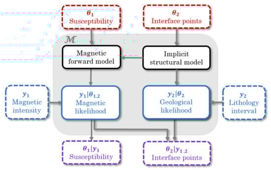
Figure 1.
The Bayesian system for our probabilistic model with prior model parameters (red); governing equations (black) that relate model parameters and observations; likelihood functions (blue); observations (blue), with being observations from magnetic measurements and from core logs; and the posterior model parameters (purple). The governing equations and the likelihood functions together form the mathematical model (grey area). Parameters are stochastic (dashed) or deterministic (solid). The arrows indicate parent-child like hierarchies.
Once the parameters to be inferred have been defined, we must choose which direct observations, y, we are going to use. In this probabilistic model, we use magnetic intensity as measured by a scalar airborne magnetometer, as well as lithology observations from core logs that are not used directly to describe the geometrical domains. These types of observations are important to be included to validate the mathematical model without increasing its complexity and hence risk overfitting.
2.3. Forward Model
The mathematical models relating the magnetic data and the geological observations to the model parameters are the interpolator functions that form the basis of our geological modeling step and the forward magnetic simulator. Essentially, this means that we consider structural geologic modeling as a forward modeling step within the Bayesian inference framework (a deeper explanation of these types of probabilistic models can be found in de la Varga and Wellmann [21] and Wellmann et al. [22]). Such an implementation requires an interpolation method that enables full automation of the geological modeling step so that a model can be updated when relevant input parameters are changed [22]. Implicit geologic modeling methods (e.g., Lajaunie et al. [26]) are well suited to represent complex geological geometries with a reduced number of parameters, and developments in recent years have shown how they can be applied to automatic model reconstruction for the evaluation of error propagation [14,15,16].
2.3.1. Implicit 3D-Modeling
Implicit interpolation has the particularity of interpolating an auxiliary dimensionless scalar field used to reconstruct the 3D spatial geometries in a post-processing step. In the case of structural geology, a helpful analogy is to think of the scalar field as a proportional field to the deposition date of an infinitesimal layer. By knowing the value of the scalar field at the interface of each domain, we can easily evaluate if a given point in space belongs to one specific domain (e.g., specific layer) or other.
The first step of any interpolation is to find a function which, upon evaluation, will yield the value of interest—the dimensionless scalar field in this case. One proven method in structural geology to obtain the interpolation function is based on surface interface points and orientation measurements using universal co-kriging [27]:
where is the gradient covariance-matrix; the covariance-matrix of the differences between each interface point and reference point in each layer; encapsulates the cross-covariance function; and are the drift functions and their gradient, respectively. The remaining terms correspond to the interpolation weights and drift coefficients , and the covariance vector between the data and the point to be interpolated (see de la Varga et al. [28] Chapter 2.1.2. for a further analysis of the system of equations).
Once we have a function capable of evaluating the value of the scalar field—and in turn its lithology and associated petrophysics—the next step is to interrogate the area of interest depending on the specific question we are trying to answer. Naturally, for a first visualization of the structures and general insights, regular grids could provide the simplest alternative to start understanding the geometries. However, it is important not to forget that implicit interpolations are meshless and therefore we can take advantage of this.
Magnetic responses decline following an inverse cube law with distance, making the contribution of zones further apart from the measurement device less and less significant. For this reason, it is more important to capture variations in the subsurface in the areas close to the device rather than further away. Since computing the forward magnetic response is a costly operation that scales super-linearly with the number of used prisms, we can optimize the location of the prisms by exploiting the flexibility that implicit interpolation enables. Instead of evaluating the structural model on a regular grid, we will create semi-spheres around the devices used for the Bayesian interpolation (i.e., the observation locations where we evaluate the likelihood of the observations ). This semi-sphere will be in turn formed by prisms that will be used for the subsequent forward geophysical calculation (Figure 2). Furthermore, the density of the prism will be reduced proportionally to the distance, making the prisms bigger and bigger as they are further away from the source in the interest of keeping the contribution of each individual prism somewhat similar.
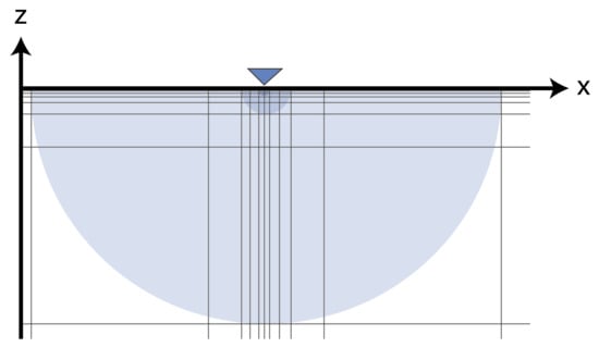
Figure 2.
A 2D representation of the grid where the forward magnetics are built on. The observation point (purple) is at the center of the grid. From here, the grid spacing increases with a distance squared relationship. The magnetic field decreases cubically with distance as shown by the blue hemispheres.
After the 3D space has been discretized and each prism has been assigned a rock unit (i.e., lithology), we can map to each lithology its correspondent petrophysical unit—the magnetic susceptibility for the model here described.
2.3.2. Magnetic Forward Modeling
Additionally, the forward magnetic computation is a required step for a coupled geophysical–geological inversion. By embedding this step into a Bayesian inference, the initial input data for the model will be conditioned to the final magnetic response. Each observation that we add to our model, encapsulated by a likelihood function, will require an additional call to the forward model in each iteration step. This forward computation is a computationally expensive task. Depending on what we want to resolve and the nature of the used data, different forward model(s) will be employed (Figure 1). If we only invert for the petrophysical rock property, we only require magnetic data and the magnetic forward model. In a similar way, we can proceed when only considering parameters of the geological model as uncertain. But if we consider both, the geological input parameters and petrophysical properties as stochastic, we automatically employ both the magnetic and structural forward model since variability in geologic input parameters changes the geological model, which influences the magnetic response of the model.
For the computation of the magnetic forward simulation, we use a voxel-based numerical implementation of the magnetic response as described by Talwani [29], which starts off with the magnetic scalar potential of an element volume :
where is the magnetization in SI units [24], a sum of induction due to an external magnetic field , and remanent magnetization due to the history of the material ; is the displacement vector from the volume to the observation point; and . By considering an infinitesimal volume, , the summation transforms into an integral:
Assuming that currents are absent at the location of observation the magnetic field can be expressed by , and the three orthogonal components of the magnetic field of an anomalous body are [29]:
where variables to represent volume integrals [29]. The solutions of the volume integrals for the case of a prism are given by Plouff [30] (see Güdük [31] Section 4.2.3. for a more detailed documentation on their implementation).
Assumptions in this expression are:
- 1.
- Magnetization is only due to induction, so that and , where is the magnetic induction and k is the magnetic susceptibility.
- 2.
- Susceptibility k of each modeled lithological unit in the geological model is known, and homogeneous and anisotropic throughout the lithological unit.
- 3.
- The anomalous magnetic field due to local subsurface conditions is small compared to the Earth’s natural magnetic field so that the direction of the total field is said to be in the same direction as the geomagnetic field, a general assumption in magnetic prospecting [24].
With this numerical implementation the intensity of the magnetic anomaly, , can be approximated by the sum of the projections of components and along the direction of the Earth’s magnetic field as expressed by the declination D and inclination I [24,29,32]:
2.4. Bayesian Inference
When setting up a Bayesian inference problem with N unknowns, we implicitly create an N-dimensional model space for the prior and posterior distributions to exist in [33]. As mentioned before, with increasing dimensions computing the evidence quickly becomes intractable and Equation (1) needs to be approximated.
2.4.1. Markov Chain Monte Carlo
Monte Carlo methods numerically approximate integrals that are not tractable analytically, but for which evaluation of the function being integrated is tractable [34]. The goal is to reconstruct the posterior (i.e., the target distribution) by going through a large number of samples, without affecting the distribution through the sampling process. To do so, a Markov chain Monte Carlo (MCMC) can be used. A Markov chain describes a sequence of points in the model space while preserving the target distribution [35]. By increasing the complexity of a given model, the number of unknowns in the model grows. The resulting high-dimensional model spaces tend to be mostly empty, and regions with high probability occupy small volumes [36] with a characteristic geometry [37]. Typical MCMC algorithms explore the model space randomly and often require small changes between each sampling step. This becomes highly inefficient in high-dimensional problems.
2.4.2. Gradient-Based MCMC Sampling
Hamiltonian Monte Carlo (HMC) efficiently explores the target distribution, by approximating the integral in the areas of interest rather than throughout the whole model space [35]. HMC is a gradient-based MCMC algorithm that abolishes random walk behavior, reduces sensitivity towards correlated input parameters, and takes advantage of the geometry of the target distribution [37]. HMC takes a series of steps informed by first-order gradient information of the input parameters called Hamiltonian trajectories [38]. These steps are combined with random walks where the next parameter values are selected via multinomial sampling with a bias towards the latter half of the taken steps in the trajectory [35]. Where HMC’s sampling efficiency is highly sensitive to the selected tuning parameters, the novel No-U-Turn Sampler (NUTS) is an extension to HMC that requires no hand-tuning [38]. NUTS is thereby currently the most efficient sampler available (for a precise definition of the NUTS algorithm see Homan and Gelman [38]). In this paper, for the first time in geological inversion, we use NUTS to analyze our coupled model.
2.4.3. Automatic Differentiation
The efficiency of NUTS allows for the use of more complex models compared to other samplers. However, since NUTS uses first-order gradient information to obtain information about the direction of the target distribution, the computation of the first-order derivative of our model is required at each sampling step. For this purpose, we use automatic differentiation (AD). AD allows efficient and accurate evaluation of derivatives of complex numeric functions with a large number of parameters, expressed as computer programs [39]. It decomposes these programs in a sequence of elementary arithmetic operations and uses the chain rule to find the model’s derivative with respect to its initial parameters. Effectively we thus need to compute the derivatives of our model with respect to all its input variables in a single flow. This requires a differentiable, fully-coupled Bayesian network. Typically in structural modeling, transitions between different geological formations—and with that their assigned (petrophysical) properties—are modeled as sharp transitions. To obtain gradient information, however, we require continuous model parameters. Therefore we smooth these transitions slightly to guarantee continuity of the gradient. By providing non-zero gradients, we can integrate the fully-coupled structural geological and geophysical model into a Bayesian inverse framework and we can utilize NUTS to efficiently sample the posterior distribution.
3. Application to the Kevitsa Deposit
We investigate the Kevitsa instrusive complex, a Nickel (Ni), Copper (Cu), and Platinum-group elements (PGE) mineralization-containing deposit located approximately 140 km North of the Arctic circle in Finnish Lapland. The deposit has a large economic significance with a proven 160 million tons of Nickel. This has led to the acquisition of extensive geophysical and geological data sets spanning several decades, yet the geometry of the intrusive body is still not well recovered. This makes it an excellent showcase for our methodology.
3.1. Geological Setting
Since its discovery in 1987 and after a first extensive study [40], numerous studies have focused on different aspects of the deposit, including geochemical modeling [41], seismic interpretation [42], and remanent magnetization assessment [43]. The Kevitsa intrusion is located within the Central Lapland greenstone belt (CLGB), which consists of several volcano-sedimentary stratigraphic groups that have undergone multiple episodes of folding and thrusting and contain ultramafic intrusives [44]. A detailed description of the regional geology is provided by Hölttä et al. [45]. The ore body is hosted in the center of the main ultramafic unit of the Kevitsa layered intrusion, which mainly consists of olivine pyroxenite and its derivatives grouped as ultramafic pyroxenite (UPX). It has an arcuate shape at the surface with a Southwest dip (Figure 3). Analysis of 2D and 3D seismic data [42] as well as borehole data suggest a deeper continuation of the Kevitsa intrusion toward the South–Southwest where it is expected to extend to over 1.5 km in depth. Here gabbroic rocks (IGB) overlay the intrusion. The thickest drill core intersection of the gabbroic rocks gives a thickness of circa 800 m. The grouped IGB unit includes magnetite gabbro, which may contain abundant equant magnetite [40]. A dunite body (UDU) crops out in the central part of the intrusion.
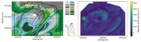
Figure 3.
(Left) Geological surface map of the Kevitsa deposit with the described units (after Fournier [46]), and the location of Kevitsa in Finland and in the Central Lapland greenstone belt (CLGB) (in green). (Right) Original airborne magnetic data with the measured total magnetic intensity.
3.2. Field Data
As geophysical observations, we use airborne magnetic data. This contains fewer effects from temporal variations and near-surface geologic sources than ground magnetics [24]. Since we are interested in recovering the geometry of the intrusion, smaller-scale variations are considered irrelevant. The dataset is acquired with a scalar magnetometer which measures the total magnetic intensity (i.e., the geomagnetic field plus anomalous field). The raw dataset is corrected for the acquisition configuration and diurnal variations and is micro-leveled. The obtained data (Figure 3) show small-scale variations within the intrusion, as well as a strong anomaly at the center of the central dunite (UDU). Core samples from this location indicate strong remanent magnetization with an unknown direction [43]. Since our forward magnetic model calculates the anomalous field (Equation (6)), we need to remove the regional field from the total-field measurements. Different methods exist for this correction [47,48] and in the absence of a general trend within the survey area, we choose to remove a direct current (DC) offset by selecting a zone where the anomalous field is expected to be zero based on geologic knowledge. Lastly, we upward-continued the data 200 m to obtain a smoother field over the intrusive body.
We represent the geology on the intrusion scale by modeling the overburden (OVB), the main intrusive body (UPX), and the host rock. The reason for this simplification is twofold: Firstly, it is uncertain which lithologies would have to be grouped without extensive petrophysical analysis of the units. The petrophysical analysis done by Fournier [46] provides a good guide but does not include all defined geological names. Secondly, we expect that all lithologies but the intrusive have little to no significant magnetic properties, except for the areas showing remanent magnetization. However, since there is no clear consensus about the direction of the remanent magnetization, the remanence cannot be captured by our forward model and the remanent regions will have to be discarded to decrease their influence on the inversion.
To build the 3D geological model, we use information from cross-sections (for the intrusive body) and core logs (for the overburden). Since there are no data regarding orientation measurements available, we are limited to a rough estimate of dips and azimuths from cross-sections. We extend our geological model further than the area of interest to avoid boundary effects in the forward magnetic calculations. We find the study-specific parameters for the geomagnetic field at the time of acquisition to be nT [49] and use these in our forward calculations (Equation (6)). Lastly, we assign a susceptibility to each of modeled lithology to simulate the magnetic response of our geological model. We use downhole susceptibility measurements along 279 boreholes and couple them to the defined lithologies from core logs at the measurement intervals. We recognize that this is error-prone and poses high uncertainties and take this into account in the analysis. We remove outliers and all values smaller than a susceptibility of . The lithologies are then grouped again according to the grouping by Fournier [46] to find representative susceptibilities for the intrusion and the host rock (Figure 4). For the overburden we consider zero susceptibility.
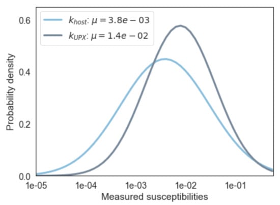
Figure 4.
Probability density function (pdf) of downhole measured susceptibilities representing the modeled lithologies ultramafic pyroxenite (UPX) and host rock. Note the logarithmic x-axis.
3.3. Defining the Probabilistic Model
We start with our initial geological model and include uncertainty in the subsurface structure. Due to the highly structurally deformed geological setting, we expect significant uncertainty in all spatial directions. We define the -coordinates of all interface points for our geological model as stochastic parameters, with normal distributions around the initially modeled contact points. We allow for large standard deviations for the intrusive body, in order to explore a wide variety of structural models. From our prior model (Figure 7a–c), we see a significant discrepancy between the observed magnetic response and the forward modeled response (Figure 7b). To understand this better, we first invert for the susceptibility of the intrusion keeping the structural geometry fixed.
With our surface-based model set-up, we assume that the susceptibility is homogeneous within each modeled lithology. By simplifying the model, we can initially assume a significant correlation among nearby observation points. To maximize the amount of information per observation, we identify points that are less correlated with each other (Figure 5). When selecting observations to recover the susceptibility of the intrusion, we consider that the measurements should represent the susceptibility variety of the intrusion without being significantly influenced by other geological structures (e.g., the central dunite and the surrounding rocks). Nor should the inversion be solely controlled by the high-mineralization zone within the intrusion. For the likelihood functions, we use a normal distribution with the mean at the forward calculated magnetic response of our geological model, which is evaluated against the measured magnetic intensity at the observation point.

Figure 5.
Processed magnetic data showing the anomalous magnetic field intensity, with the cross-section location (line) at which we evaluate our results; the locations where we evaluate the magnetic likelihood functions (filled dots); and the geological likelihood (star). We use the locations with an extra circle to invert for the susceptibility of the intrusion.
Due to the large discrepancy between the observed magnetic response and the initial forward model (Figure 7b), we can state that we have no reasonable initial guess of the susceptibility of the intrusion. Therefore, we assign a uniform distribution to it, indicating that all values within the specified range are equally probable. We can analyze the joint ensemble from all three observations by looking at the prior (and posterior) predictive distributions. These are constructed by passing samples from the joint prior (or posterior) parameter distribution through the forward model and simulating data given those parameters. This allows us to quantify how likely it is that we can simulate the measured data given our prior (or posterior) parameters. We can see from Figure 6 that is recovered well, as its posterior distribution provides forward simulated magnetic responses that match the observed response.
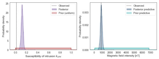
Figure 6.
(Left) Pdf with prior and posterior distribution of , and the mean of the downhole measured susceptibility for (dashed line). (Right) Pdf with prior and posterior predictive distribution as simulated at one of the observation locations, and the measured magnetic intensity at that observation location (dashed line).
With the updated knowledge about the magnetic susceptibility, we assign the obtained posterior distribution of (Figure 6) as the prior distribution for further model analysis. We use the measured values for the host rock () and define , both as constant values. To update our prior model in the light of observed data, well-defined likelihood functions are needed. We initially only use geophysical likelihood functions using the measured (and processed) magnetic data. Since the forward computation is expensive, we limit our inversion to selected uncorrelated observations rather than considering all points on the entire grid. The selection of meaningful measurement points is based on expert knowledge by selecting magnetic measurement locations that will minimize the correlation and maximize the objective of the inversion, i.e., the retrieval of the geometry. Most observations points are therefore chosen around the magnetic anomaly (Figure 5, filled dots).
At greater depths, the magnetic field becomes too weak to provide a meaningful and informative likelihood function. To estimate the geometry at these depths, we can use other constraints that are more informative at greater depths. To illustrate this, we extend our inference framework by adding a geological likelihood based on interpreted core logs at a location where the seismic data analysis expected the bottom of the intrusion to reach approximately 1500 m [42]. The geological likelihood is incorporated to the inference by adding the -coordinates of the borehole where the bottom of the intrusion is logged as the observation. We define the likelihood by using a normal distribution, with the mean value being the forward modeled geological unit at the grid point.
3.4. Analysis of Model Uncertainties
Figure 7 shows the different components of our analyses. The first column corresponds to our initial model. The rows show (from top to bottom) a cross-section; the difference in magnetic response between the magnetic measurements and the forward model; the same cross-section where we visualize the uncertainties in our initial geological using information entropy [19]. The uncertainties in our initial structural model are based on expert knowledge, and within these assigned ranges, different structural models can be realized. We realized 500 different geological models.
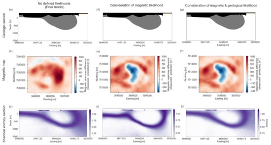
Figure 7.
(a) Cross-section of the initial model; (b) difference map between the forward modeled magnetic response of the initial model and the magnetic measurements; (c) calculated entropy from all realized models based on assigned uncertainty in the initial model, where zero (white) corresponds to locations with no uncertainty (i.e., locations that have the same outcome in all realizations). (d) Cross-section of the Maximum A Posteriori (MAP) geological model based on magnetic constraints; (e) difference between the forward modeled magnetic response of the MAP model and the magnetic measurements; (f) calculated entropy from all realized models in the probabilistic inversion using only magnetic likelihoods. (g) Cross-section of the MAP model based on magnetic and additional geological constraints; (h) difference between the forward modeled magnetic response of the MAP model and the magnetic measurements; (i) calculated entropy from all realized models in the probabilistic inversion using magnetic and geological likelihoods.
By using information entropy we can consider all these realized models and objectively visualize them. We apply this concept by slicing a 2D section from our 3D model and dividing this cross-section into cells. It is important to note here that this cell splitting does not affect the realized geological models or inversion results and only affects the resolution of this figure. We compute the probability of each modeled lithology to occur in a particular cell by combining all 500 models. The obtained scalar value at each cell represents the uncertainty at that point in space. In analogy to entropy in thermodynamics, high entropy indicates high disorder and thus larger uncertainties. Zero entropy implies no uncertainty: in all realized models the same lithology occurred at that point in space. On the other hand, when all modeled lithologies are equally likely to occur at a point, we have maximum entropy , where n is the number of modeled formations.
The second column shows the results of our inversion with magnetic likelihood functions, where we used the obtained posterior susceptibility distribution to update our prior (Figure 6). To show a cross-section and magnetic difference map from a model out of the realized model ensemble, we use the Maximum A Posteriori (MAP) estimation. This provides the model that statistically fits the observed data best. The difference in the structural model is very small (Figure 7d compared to a), but the magnetic difference map is significantly different than our prior model with the measured susceptibility values (Figure 7e compared to b). In our initial difference map we mostly see an effect of the susceptibility, but the better estimate of the susceptibility makes a structural effect visible in the updated difference map. For the computation of the entropy (Figure 7f) we use the similar resolution as before, and again analyze 500 realized geological models. These are constructed using posterior model parameters from samples after (expected) convergence to the target distribution.
From geological knowledge, it is expected that the body extends deeper than it does in our geological model. For this purpose, we included the geological likelihood. The results are shown in the third column. We see that the MAP model does not change the magnetic response noticeably (Figure 7e,h) and the structural MAP model shows no noticeable change (Figure 7d,g compared to a). When we consider the ensemble of all realized models, we do see differences in the structural models ((Figure 7c,f,g). The prior model shows high uncertainty towards the East and regions with increased entropy at larger depth. In Figure 7f, entropy has overall decreased, particularly in the East where magnetic forward predictions show a better fit to the data as well (Figure 7e compared to b). However, the effects of some increased entropy at depth remain. It looks like these regions show individual bulbs, disconnected from the main intrusive body. Based on geologic knowledge, it is not expected that these features are representative of the subsurface structures and that they violate the expected topology in the domain [50]. We therefore interpret these effects as possible artifacts. We see in Figure 7i that adding a geological likelihood poses indeed a better constraint at this depth and removes the artifacts, even though the added borehole data are approximately 700 m South of this section. Overall the uncertainty in the section has increased, due to an increased uncertainty to the East. This is expected to be due to competing prior and likelihood functions (see Discussion).
The high entropy at the interface between intrusion and the overburden in all sections is a result of the small thickness of the overburden in combination with the resolution of the grid on which the entropy is calculated. Since the overburden is so thin (and stochastic), the occurring formation in a cell in these zones interchanges quickly per sample, and hence both the overburden and UPX have a probability to occur in a particular cell and the resulting entropy is high.
3.5. Numerical Implementation
In this study, we used programs written in the high-level programming language Python (3.6). We built the geological model using GemPy [28], a 3D geological modeling tool based on the implicit modeling methodology discussed in Section 2.3.1. We coupled this to our implementation of the magnetic forward modeling step, as described in Section 2.3.2. We computed the gradients of our coupled geological and magnetic forward model via AD from library Theano [51]. For the inference, we used the probabilistic programming framework PyMC3 [52], which contains efficient gradient-based MCMC samplers, including NUTS. PyMC3 also relies on Theano for AD and is therefore compatible with our forward model. For reputability of the entire modeling workflow, we made the entire processing workflow available on GitHub (https://github.com/cgre-aachen-papers/probabilistic-inversion-magnetics-kevitsa/ accessed on 22 January 2021).
4. Discussion
Bayesian inference enables information integration and uncertainty quantification in one framework: a necessity for modeling the subsurface where uncertainties are often significant and data should be considered in context. Considering geological information in combination with geophysical measurements in an inverse framework is not new [14,53,54,55,56,57], nor is the idea of explicitly considering geological models as uncertain [14,15,16,58]. Our method of including geological modeling as part of the Bayesian inference framework [21,22], and implementing geophysical information to the geological model in the form of likelihood functions has also been tested before [22]. The novelty here is that we used the most efficient MCMC sampler (NUTS) currently available by computing the gradient of our coupled geological-geophysical model. This implementation allows increasing the complexity of a model and thereby opens up interesting possibilities. In our application we also, different from previous work, consider both the structural model and the relevant petrophysical rock property as uncertain. We applied this to a case study of the Kevitsa intrusion in Finland. Through the use of our model-based Bayesian inference framework, we found discrepancies in the data that otherwise might have gone unnoticed. Additionally, we show that in contrast to conventional inversions that require a regular grid, our method improves the selection of observation locations—for a given model— because of the constraints set by the prior geometry. It thereby allows us to allocate computational resources effectively.
We would also like to emphasize the difference between the model-based geological and geophysical joint inversion implemented here to other approaches. The conceptual idea behind the use of geological models in geophysical inverse approaches is described in detail in Wellmann and Caumon [7]. In our case, the geological model is a fully integrated part of the Bayesian inference workflow. We can therefore obtain posterior probability distributions for the initial parameters of the geological model, and we can guarantee that all realizations fulfill the initial considerations of the geological interpolation approach. This approach is different from widely used methods where the geological model is an input to the geophysical inversion (e.g., [55,56,59]), or more recent approaches that consider uncertainties in the geological model through a pre-computation of cell-based lithological probabilities [60,61]. Another important difference is in how the different approaches deal with is the natural spatial correlation in geological and geophysical data [21]. Inverting on a regular (dense) grid and considering the rock property in each cell as a separate parameter is a high-dimensional problem with a high correlation between parameters, where each one in itself is relatively uninformative. In such solely data-driven geophysical inversion approaches, it is often necessary to use regularization [46,62,63,64]. In our implementation, regularization is not needed, and with the geological model as the basis of the inversion, we have a relatively low-dimensional model parameterization and, ideally, only a small correlation between parameters. The choice between these more geophysical data-driven approaches compared to the geomodel-based inversions clearly depends on the focus of the study and the available prior information. A more integrated combination of both viewpoints is an interesting aspect for further research.
In our case study, we simplified the geology considerably. In the results, we observed that the geological model was partly too simplified to capture the data complexity. The thick gabbroic layer that overlays the intrusion towards the Southwest has significantly different magnetic properties than the intrusion. To capture the structures there, the gabbroic rock has to be considered too. The complexity in including the gabbro lies in the heterogeneity of the formation. It contains significant amounts of magnetite gabbro with stronger magnetic properties than the rest of the rock. Similarly, the intrusive body itself shows considerable heterogeneity in rock properties. This is also observed from seismic data [42] and is expected to be due to internally differentiated olivine pyroxenite pulses. Since geophysical measurements reflect rock property contrasts, our model could be improved by extending to a heterogeneous inversion. However, this would require an extensive petrophysical study, and even then it would be complicated to capture the individual pulses within the intrusion [42].
We try to take the heterogeneity in susceptibility within the intrusion into account, by considering it as a stochastic parameter. Considering the mismatch in magnetic response between our initial forward simulation and the observed data (Figure 7b), we can conclude that our initial (measured) estimate of the susceptibility of the intrusion could not describe the magnetic measurements. Since our inversion will mainly depend on magnetic likelihoods, we stress the importance of an appropriate initial estimate of the susceptibility to be vital for the success of our inversion. Therefore we inverted for the susceptibility using a completely uninformative prior distribution and very informative likelihoods, rather than directly combining it within a more complex probabilistic model. We verified the obtained mean value () by forward modeling over the intrusion using the commercial software package ModelVision [65] (). The mismatch with the mean borehole measured susceptibility is an order of magnitude (). Although the large dispersion in the susceptibility data (Figure 4) suggests that there is at least some effect of uncertainties due to core logging and upscaling, it is unlikely that alone would cause such a significant difference. A study by Adams and Dentith [66] provides a more likely explanation. The authors compare susceptibility measurements from conventional hand-held susceptibility instruments, like our measurement device, to measurements with a tool that considers natural remanent magnetization and conclude that the exclusive use of these measured susceptibilities for the interpretation of magnetic data is questionable. Their study shows that conventional hand-held devices under-report susceptibility values in remanent rocks with discrepancies up to several orders of magnitude. Other studies with hand-held susceptibility meters show considerable effects due to self-demagnetization [67], thermal conditions [68], and rock heterogeneity [69]. Considering these sensitivities in conventional susceptibility measurements, the complex setting of our case study, and the known occurrence of remanent magnetization, we assume that the susceptibility data were incorrect and consider it justified to continue our analysis with the inverted susceptibility.
We initially also attempted to invert for the susceptibility of the host rock in a similar way. The obtained posterior gave a mean value close to the susceptibility found from measurements ( and respectively); however, inversion statistics indicated that the MCMC algorithm did not converge, which is likely due to the oversimplification in defining the host rock. Due to the poor understanding of the actual distribution, it was decided to not include the susceptibility of the surrounding rock as a stochastic parameter. This is justified by considering (1) the small magnetic effect of the host rock relative to the intrusion due to the two-order-of-magnitude larger , (2) the aim of our case study to focus on the intrusion, and (3) the defined likelihood functions: the selected magnetic observation are all in the vicinity of the intrusion.
An interesting feature from our analysis is that adding more constraints (i.e., likelihood functions), does not necessarily reduce the uncertainty in our model (comparing Figure 7f,i). This result is also observed by Wellmann [22] and is in line with the concept of integrating information through additional information. Additional information can lead to an increase in uncertainty due to a lack of prior knowledge in combination with a poorly-defined likelihood, or due to incompatibility between priors and likelihoods. We expect that our geological likelihood was well defined, but was possibly incompatible with our prior model. It is entirely possible, or in fact expected, that our initial structural model was incorrect at greater depths, and that the magnetic likelihoods could not resolve this aspect. We expect that the incorrect initial model was only adjusted at these depths through the geological likelihood, capturing the uncertainty there. This localized higher uncertainty to the East is also in-line with findings from seismic studies where interpretation becomes more ambiguous towards the East [42]. More informative geological likelihoods could be added in this way. We limited our geological likelihood to one since this was currently the only borehole available that exited the intrusion at greater depths in this area and thus could provide the constraint that our model required.
It is important to note that we aimed to use different data types and combine their respective strengths. The used data should be considered in light of what we want to gain from the inversion. When we are interested in geological structures, potential field data do not provide enough information. The inherent non-uniqueness of potential fields is due to the physical inability to distinguish between different geometries at different depths. More meaningful geophysical constraints could be imposed by using e.g., seismic data. The complexity here is that seismic data are often not well understood in mineral exploration settings. Although seismic data from Kevitsa are available, it suffers from problems commonly seen in these settings: the data are within an extremely high-velocity environment and the velocity is also extremely variable [42]. A better understanding of the data and proper processing is needed before it can be used in our framework. The ambiguity in its interpretation (dips and spatial positions of the interpreted surfaces) due to a lack of suitable velocity model [42] is also why we decided to build our initial geological model on cross-sections rather than the seismic interpretation.
Lastly, we want to state the importance of using a balanced palette of observations in the probabilistic inference, while also balancing geological reality and data fitting in the implementation. This is best illustrated by computing the MAP and obtaining the model that maximizes the joint posterior distribution. Since we mostly used magnetic likelihoods in our application, the susceptibility had a dominant contribution in our model. This was clear from the MAP models (Figure 7f,i), which gave us a geological model that statistically fitted best because effectively, the susceptibility fit was maximized. The MAP, in this case, did not provide any information about the weaker spatial parameters and the structural model remained close to the initial model. It should also be mentioned that in high-dimensional problems the maximized joint posterior distribution is often not where the probabilistic mass is accumulated, and the obtained MAP models are therefore not exclusively representative for the target ensemble of models [35]. We can conclude that: (1) to fully make use of the strengths of different sources we should aim for the use of different likelihoods where no parameter is dominating the inversion; (2) a statistical fit does not necessarily give a result that represents the geology. Following Occam’s razor, we should aim to keep the model as simple as possible while trying to fit the data, rather than adjusting the model to fit the data.
To summarize, we aim to provide a step forward on data integration and quantitative analysis to unravel the subsurface. Both geological modeling and geophysical interpretation are subjective practices influenced by the expert, and the same holds for building a Bayesian model. Yet quantifying uncertainties in input parameters and measurements enables communication and consideration of our subjective choices and the encountered uncertainties, which we can then represent in the final geological model.
Author Contributions
Conceptualization, F.W. and M.d.l.V.; methodology, N.G., F.W., J.K., and M.d.l.V.; software, M.d.l.V. and N.G.; validation, J.K., N.G., and F.W.; investigation, N.G. and J.K.; resources, F.W.; writing—original draft preparation, N.G.; writing—review and editing, N.G., F.W., and M.d.l.V.; visualization, N.G.; supervision, F.W., J.K., and M.d.l.V.; project administration, F.W.; funding acquisition, F.W. and J.K. All authors have read and agreed to the published version of the manuscript.
Funding
This project has received funding from the European Institute of Innovation and Technology—Raw Materials—under grant agreements No. 16258 and No. 19004, and by Boliden Mines.

Institutional Review Board Statement
Not applicable.
Informed Consent Statement
Not applicable.
Data Availability Statement
Not applicable.
Acknowledgments
We are grateful for the support by Boliden Mines in the organization and administrative support of the case study to enable field and data access.
Conflicts of Interest
The authors declare no conflict of interest. The funders had no role in the design of the study; in the collection, analyses, or interpretation of data; in the writing of the manuscript, or in the decision to publish the results.
References
- Lelievre, P.; Carter-McAuslan, A.; Farquharson, C.; Hurich, C. Unified geophysical and geological 3D Earth models. Lead. Edge 2012, 31, 322–328. [Google Scholar] [CrossRef]
- Ellis, R.G.; MacLeod, I.N. Constrained voxel inversion using the Cartesian cut cell method. ASEG Ext. Abstr. 2013, 1, 1–4. [Google Scholar] [CrossRef]
- Özyıldırım, Ö.; Candansayar, M.E.; Demirci, İ.; Tezkan, B. Two-dimensional inversion of magnetotelluric/radiomagnetotelluric data by using unstructured mesh. Geophysics 2017, 82, E197–E210. [Google Scholar] [CrossRef]
- Sheldon, H.; Micklethwaite, S. Damage and permeability around faults: Implications for mineralization. Geology 2007, 35. [Google Scholar] [CrossRef]
- Okamoto, A.; Tsuchiya, N. Velocity of vertical fluid ascent within vein-forming fractures. Geology 2009, 37, 563–566. [Google Scholar] [CrossRef]
- Gallardo, L.; Thébaud, N. New insights into Archean granite-greenstone architecture through joint gravity and magnetic inversion. Geology 2012, 40, 215–218. [Google Scholar] [CrossRef]
- Wellmann, F.; Caumon, G. 3-D Structural geological models: Concepts, methods, and uncertainties. In Advances in Geophysics; Elsevier: Amsterdam, The Netherlands, 2018; Volume 59, pp. 1–121. [Google Scholar]
- Gelman, A.; Carlin, J.B.; Stern, H.S.; Rubin, D.B. Bayesian Data Analysis, 3rd ed.; Chapman and Hall/CRC: London, UK, 2013; p. 675. [Google Scholar]
- MacKay, D.J.C. Information Theory, Inference, and Learning Algorithms; Copyright Cambridge University Press: Cambridge, UK, 2003. [Google Scholar]
- Tarantola, A.; Valette, B. Inverse Problems = Quest for Information. J. Geophys. 1982, 50, 159–170. [Google Scholar]
- Mosegaard, K.; Tarantola, A. Monte Carlo sampling of solutions to inverse problems. J. Geophys. Res. 1995, 1001, 12431–12448. [Google Scholar] [CrossRef]
- Sambridge, M.; Mosegaard, K. Monte Carlo methods in geophysical inverse problems. Rev. Geophys. 2002, 40, 1009. [Google Scholar] [CrossRef]
- Betancourt, M.J.; Byrne, S.; Livingstone, S.; Girolami, M. The Geometric Foundations of Hamiltonian Monte Carlo. arXiv 2014, arXiv:1410.5110. [Google Scholar] [CrossRef]
- Jessell, M.; Ailleres, L.; Dekemp, E. Towards an integrated inversion of geoscientific data: What price of geology? Tectonophysics 2010, 490, 294–306. [Google Scholar] [CrossRef]
- Wellmann, F.; Horowitz, F.; Schill, E.; Regenauer-Lieb, K. Towards incorporating uncertainty of structural data in 3D geological inversion. Tectonophysics 2010, 490. [Google Scholar] [CrossRef]
- Lindsay, M.; Ailleres, L.; Jessell, M.; Dekemp, E.; Betts, P. Locating and quantifying geological uncertainty in three-dimensional models: Analysis of the Gippsland Basin, southeastern Australia. Tectonophysics 2012, 546-547, 10–27. [Google Scholar] [CrossRef]
- De la Varga, M.; Wellmann, F.; Murdie, R. Adding geological knowledge to improve uncertain geological models: A Bayesian perspective. Geotecton. Res. 2015, 97, 18–20. [Google Scholar] [CrossRef]
- Lindsay, M.; Jessell, M.; Ailleres, L.; Perrouty, S.; Dekemp, E.; Betts, P. Geodiversity: Exploration of 3D geological model space. Tectonophysics 2013, 594. [Google Scholar] [CrossRef]
- Wellmann, J.F.; Regenauer-Lieb, K. Uncertainties have a meaning: Information entropy as a quality measure for 3-D geological models. Tectonophysics 2012, 526-529, 207–216. [Google Scholar] [CrossRef]
- Wellmann, F.; Lindsay, M.; Poh, J.; Jessell, M. Validating 3-D Structural Models with Geological Knowledge for Improved Uncertainty Evaluations. Energy Procedia 2014, 59, 374–381. [Google Scholar] [CrossRef]
- De la Varga, M.; Wellmann, J.F. Structural geologic modeling as an inference problem: A Bayesian perspective. Interpretation 2016, 4, SM1–SM16. [Google Scholar] [CrossRef]
- Wellmann, J.F.; de la Varga, M.; Murdie, R.E.; Gessner, K.; Jessell, M. Uncertainty estimation for a geological model of the Sandstone greenstone belt, Western Australia—Insights from integrated geological and geophysical inversion in a Bayesian inference framework. Geol. Soc. Lond. Spec. Publ. 2018, 453, 41–56. [Google Scholar] [CrossRef]
- Telford, W.M.; Telford, W.; Geldart, L.; Sheriff, R.E.; Sheriff, R.E. Applied Geophysics; Cambridge University Press: Cambridge, UK, 1990; Volume 1. [Google Scholar]
- Hinze, W.J.; von Frese, R.R.B.; Saad, A.H. Gravity and Magnetic Exploration: Principles, Practices, and Applications; Cambridge University Press: Cambridge, UK, 2013. [Google Scholar] [CrossRef]
- Tarantola, A. Inverse Problem Theory and Methods for Model Parameter Estimation; Society for Industrial and Applied Mathematics: Philadelphia, PA, USA, 2005. [Google Scholar] [CrossRef]
- Lajaunie, C.; Courrioux, G.; Manuel, L. Foliation fields and 3D cartography in geology: Principles of a method based on potential interpolation. Math. Geol. 1997, 29, 571–584. [Google Scholar] [CrossRef]
- Chiles, J.P.; Delfiner, P. Geostatistics: Modeling Spatial Uncertainty; John Wiley & Sons: Hoboken, NJ, USA, 2009; Volume 497. [Google Scholar]
- De la Varga, M.; Schaaf, A.; Wellmann, F. GemPy 1.0: Open-source stochastic geological modeling and inversion. Geosci. Model Dev. 2019, 12, 1–32. [Google Scholar] [CrossRef]
- Talwani, M. Computation with the help of a digital computer of magnetic anomalies caused by bodies of arbitrary shape. Geophysics 1965, 30, 797–817. [Google Scholar] [CrossRef]
- Plouff, D. Gravity and magnetic fields of polygonal prisms and application to magnetic terrain corrections. Geophysics 1976, 41, 727–741. [Google Scholar] [CrossRef]
- Güdük, N. Model-Based Probabilistic Inversion Using Magnetic Data: A Case Study on the Kevitsa Deposit. Master’s Thesis, IdeaLeague, RWTH Aachen University, Aachen, Germany, 2020. Available online: http://resolver.tudelft.nl/uuid:f809a7ed-89e9-4e6f-abe4-e6683ba0fa78 (accessed on 2 March 2020).
- Blakely, R.J. Potential Theory in Gravity and Magnetic Applications; Cambridge University Press: Cambridge, UK; New York, NY, USA, 1995. [Google Scholar]
- Davidson-Pilon, C. Bayesian Methods for Hackers: Probabilistic Programming and Bayesian Inference, 1st ed.; Addison-Wesley Professional: Boston, MA, USA, 2015. [Google Scholar]
- Metropolis, N.; Ulam, S. The Monte Carlo method. J. Am. Stat. Assoc. 1949, 44, 335. [Google Scholar] [CrossRef]
- Betancourt, M. A Conceptual Introduction to Hamiltonian Monte Carlo. arXiv 2018, arXiv:1701.02434. [Google Scholar]
- Bellman, R. Dynamic Programming, 1st ed.; Princeton University Press: Princeton, NJ, USA, 1957. [Google Scholar]
- Neal, R.M. MCMC using Hamiltonian dynamics. arXiv 2012, arXiv:1206.1901. [Google Scholar]
- Homan, M.D.; Gelman, A. The No-U-Turn Sampler: Adaptively Setting Path Lengths in Hamiltonian Monte Carlo. J. Mach. Learn. Res. 2014, 15, 1593–1623. [Google Scholar]
- Baydin, A.G.; Pearlmutter, B.A.; Radul, A.A.; Siskind, J.M. Automatic differentiation in machine learning: A survey. arXiv 2018, arXiv:1502.05767. [Google Scholar]
- Mutanen, T. Geology and Ore Petrology of the Akanvaara and Koitelainen Mafic Layered Intrusions and the Keivitsa-Satovaara Layered Complex, Northern Finland; Bulletin (Geologian tutkimuskeskus (Finland)); Geological Survey of Finland: Espoo, Finland, 1997. [Google Scholar]
- Le Vaillant, M.; Hill, J.; Barnes, S.J. Simplifying drill-hole domains for 3D geochemical modelling: An example from the Kevitsa Ni-Cu-(PGE) deposit | Elsevier Enhanced Reader. Ore Geol. Rev. 2017, 90, 388–398. [Google Scholar] [CrossRef]
- Koivisto, E.; Malehmir, A.; Hellqvist, N.; Voipio, T.; Wijns, C. Building a 3D model of lithological contacts and near-mine structures in the Kevitsa mining and exploration site, Northern Finland: Constraints from 2D and 3D reflection seismic data: Kevitsa 3D geological model. Geophys. Prospect. 2015, 63, 754–773. [Google Scholar] [CrossRef]
- Montonen, M. Induced and Remanent Magnetization in Two Boreholes of the Kevitsa Intrusion. Master’s Thesis, University of Helsinki, Helsinki, Finland, 2012. [Google Scholar]
- Gregory, J.; Journet, N.; White, G.; Lappalainen, M. Kevitsa Nickel Copper Mine, Lapland, Finland; Technical report; First Quantum Minerals Ltd.: London, UK, 2016. [Google Scholar]
- Hölttä, P.; Väisänen, M.; Väänänen, J.; Manninen, T. Paleoproterozoic metamorphism and deformation in Central Lapland, Finland. Spec. Paper Geol. Surv. Finl. 2007, 44, 7–56. [Google Scholar]
- Fournier, D. Advanced Potential Field Data Inversion with lp-norm Regularization. Ph.D. Thesis, University of British Columbia, Vancouver, BC, Canda, 2019. [CrossRef]
- Hinze, W.J. The Role of Gravity and Magnetic Methods in Engineering and Environmental Studies. In Geotechnical and Environmental Geophysics: Volume I, Review and Tutorial; Society of Exploration Geophysicists: Houston, TX, USA, 2012; pp. 75–126. [Google Scholar] [CrossRef]
- Li, Y.; Oldenburg, D.W. Separation of regional and residual magnetic field data. Geophysics 1998, 63, 431–439. [Google Scholar] [CrossRef]
- National Oceanic and Atmospheric Administration (NOAA). Available online: https://www.ngdc.noaa.gov/geomag/calculators/magcalc.shtml#igrfwmm (accessed on 6 December 2019).
- Thiele, S.T.; Jessell, M.W.; Lindsay, M.; Ogarko, V.; Wellmann, J.F.; Pakyuz-Charrier, E. The topology of geology 1: Topological analysis. J. Struct. Geol. 2016, 91, 27–38. [Google Scholar] [CrossRef]
- Theano Development Team. Theano: A Python framework for fast computation of mathematical expressions. arXiv 2016, arXiv:abs/1605.02688. [Google Scholar]
- Salvatier, J.; Wiecki, T.; Fonnesbeck, C. Probabilistic Programming in Python using PyMC. arXiv 2015, arXiv:1507.08050. [Google Scholar]
- Li, Y.; Oldenburg, D.W. Incorporating geological dip information into geophysical inversions. Geophsysics 2000, 65, 148–157. [Google Scholar] [CrossRef]
- Wood, R.; Curtis, A. Geological prior information and its applications to geoscientific problems. Geol. Soc. Lond. Spec. Publ. 2004, 239. [Google Scholar] [CrossRef]
- Calcagno, P.; Courrioux, G.; Joly, A.; Ledru, P.; Guillen, A. Geological modelling from field data and geological knowledge: Part II. Modelling validation using gravity and magnetic data inversion. Phys. Earth Planet. Inter. Phys. Earth Planet. Inter. 2008, 171, 1–4. [Google Scholar]
- Joly, A.; Martelet, G.; Chen, Y.; Faure, M. A multidisciplinary study of a syntectonic pluton close to a major lithospheric-scale fault: Relationships between the Montmarault granitic massif and the Sillon Houiller Fault in the Variscan French Massif Central. Part II: Gravity, aeromagnetic investigations and 3D geologic modeling. J. Geophys. Res. 2008, 113. [Google Scholar] [CrossRef]
- Lelievre, P.; Oldenburg, D.; Williams, N. Integrating geological and geophysical data through advanced constrained inversions. Explor. Geophys. 2009, 40. [Google Scholar] [CrossRef]
- Jessell, M.; Ailleres, L.; Dekemp, E.; Lindsay, M.; Wellmann, F.; Hillier, M.; Laurent, G.; Carmichael, T.; Martin, R. Next Generation Three-Dimensional Geologic Modeling and Inversion. Soc. Econ. Geol. Spec. Publ. 2014, 18, 261–272. [Google Scholar] [CrossRef]
- Bosch, M.; Guillen, A.; Ledru, P. Lithologic tomography: An application to geophysical data from the Cadomian belt of northern Brittany, France. Tectonophysics 2001, 331, 197–227. [Google Scholar] [CrossRef]
- Giraud, J.; Pakyuz-Charrier, E.; Jessell, M.; Lindsay, M.; Martin, R.; Ogarko, V. Uncertainty reduction through geologically conditioned petrophysical constraints in joint inversionConditioned petrophysical constraints. Geophysics 2017, 82, ID19–ID34. [Google Scholar] [CrossRef]
- Giraud, J.; Lindsay, M.; Ogarko, V.; Jessell, M.; Martin, R.; Pakyuz-Charrier, E. Integration of geoscientific uncertainty into geophysical inversion by means of local gradient regularization. Solid Earth 2019, 10, 193–210. [Google Scholar] [CrossRef]
- Tikhonov, A.; Arsenin, V. Solution of Ill-Posed Problem; Society for Industrial and Applied Mathematics: Philadelphia, PA, USA, 1977; p. 258. [Google Scholar]
- Zhdanov, M. Geophysical Inverse Theory and Regularization Problem; Elsevier: Amsterdam, The Netherlands, 2002; Volume 36. [Google Scholar]
- Sun, J.; Li, Y. Adaptive Lp inversion for simultaneous recovery of both blocky and smooth features in a geophysical model. Geophys. J. Int. 2014, 197. [Google Scholar] [CrossRef]
- Tensor Research. ModelVision Magnetic & Gravity Interpretation System, 17 ed. 1993. Available online: http://www.tensor-research.com.au/Geophysical-Products/ModelVision (accessed on 6 December 2019).
- Adams, C.; Dentith, M. Magnetic measurements on diamond drill core: Are we really measuring magnetic susceptibility? In Proceedings of the Exploration ’17 Sixth Decennial International Conference on Mineral Exploration, Toronto, ON, Canada, 22–25 October 2017; Volume 52, pp. 725–728. [Google Scholar]
- Clark, D. Methods for determining remanent and total magnetisations of magnetic sources—A review. Explor. Geophys. 2014, 45, 271. [Google Scholar] [CrossRef]
- Schmidt, P.; Lackie, M. Practical considerations: Making measurements of susceptibility, remanence and Q in the field. Explor. Geophys. 2014, 45, 305. [Google Scholar] [CrossRef]
- Lee, M.D.; Morris, W.A. Comparison of Magnetic-Susceptibility Meters Using Rock Samples from the Wopmay Orogen, Northwest Territories; Technical Note 5; Geological Survey of Canada: Vancouver, BC, Canada, 2013. [Google Scholar] [CrossRef]


Publisher’s Note: MDPI stays neutral with regard to jurisdictional claims in published maps and institutional affiliations. |
© 2021 by the authors. Licensee MDPI, Basel, Switzerland. This article is an open access article distributed under the terms and conditions of the Creative Commons Attribution (CC BY) license (http://creativecommons.org/licenses/by/4.0/).