
Field Observations of a Multilevel Beach Cusp System and Their Swash Zone Dynamics


Abstract
1. Introduction
2. Beach Cusp Evolution
2.1. Beach Cusp Predictions
2.2. Multilevel Beach Cusp System
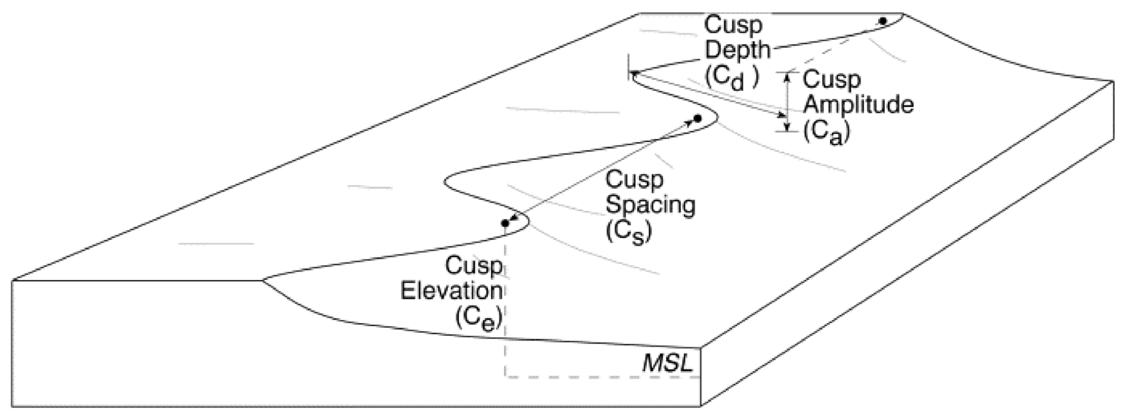
- To quantify four different cusp parameters (i.e., Cusp Spacing, Cusp Elevation, Cusp Amplitude, and Cusp Depth) of a three-tiered cusp system during a six-month period;
- To link their change over time with the hydrodynamics occurring in the study area;
- To provide insightful information regarding the current predictive formulations for cusp spacing;
- To formulate new predictive theories for the other cusp parameters (i.e., Cusp Elevation, Cusp Amplitude, and Cusp Depth).
3. Methodology
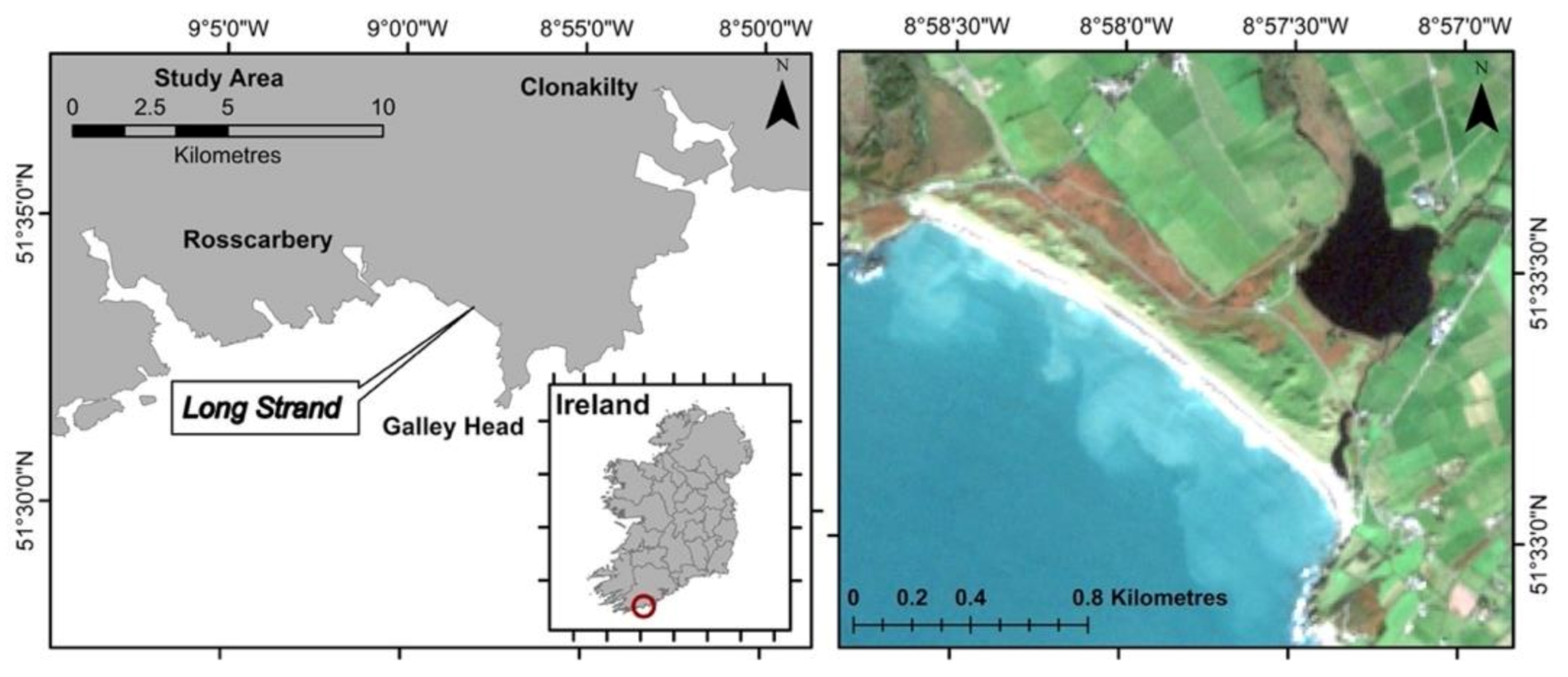
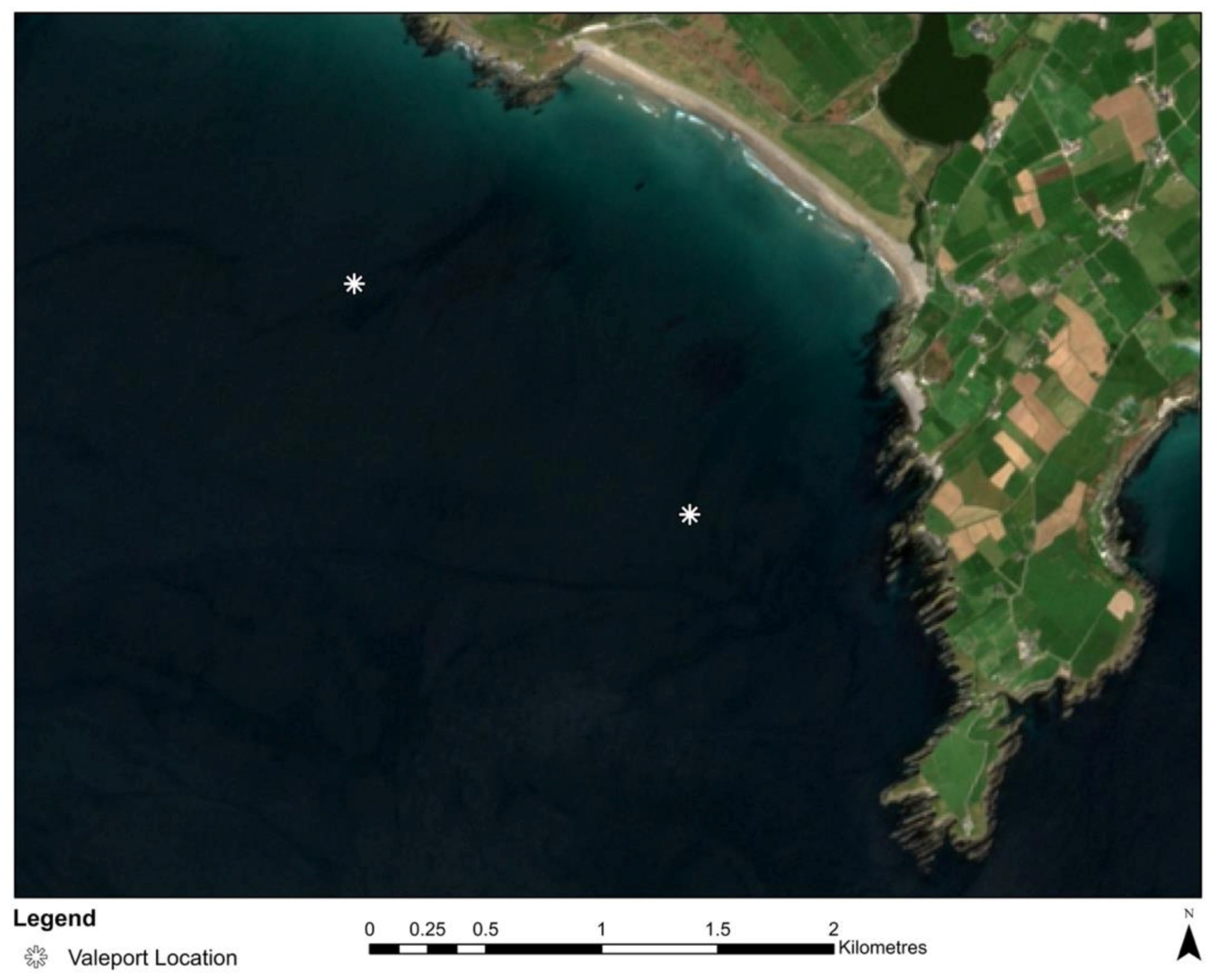
3.1. Study Area
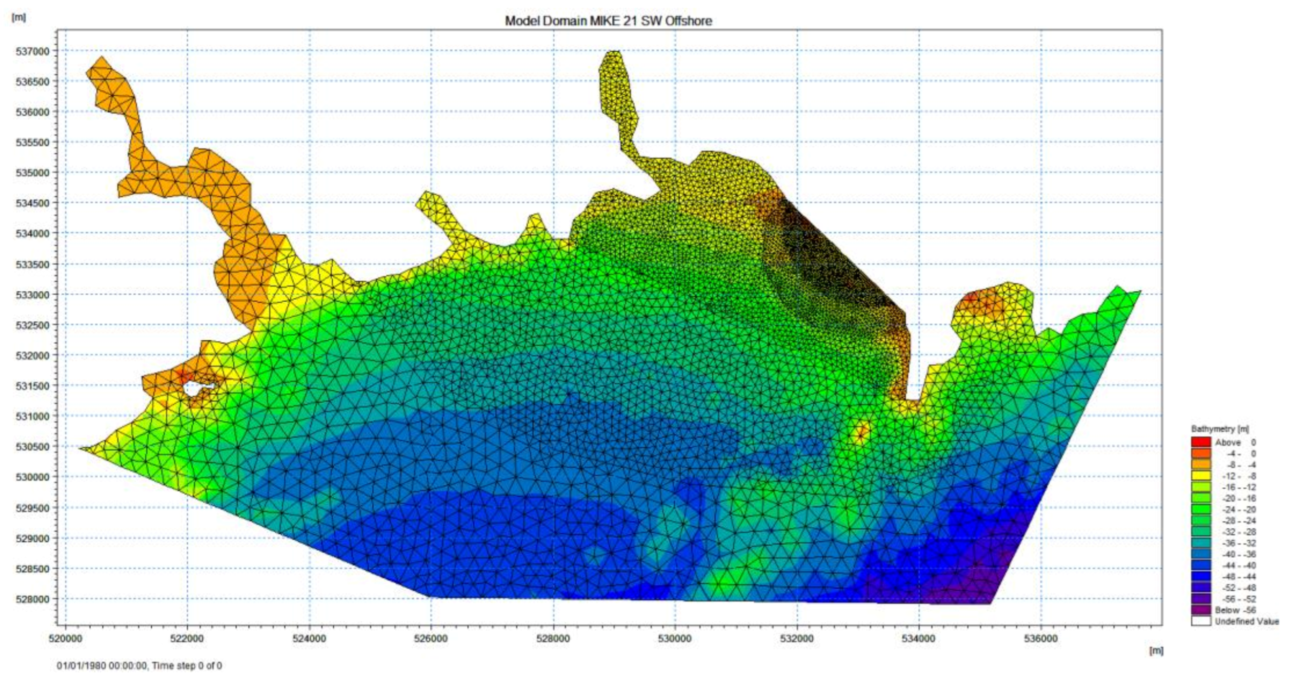
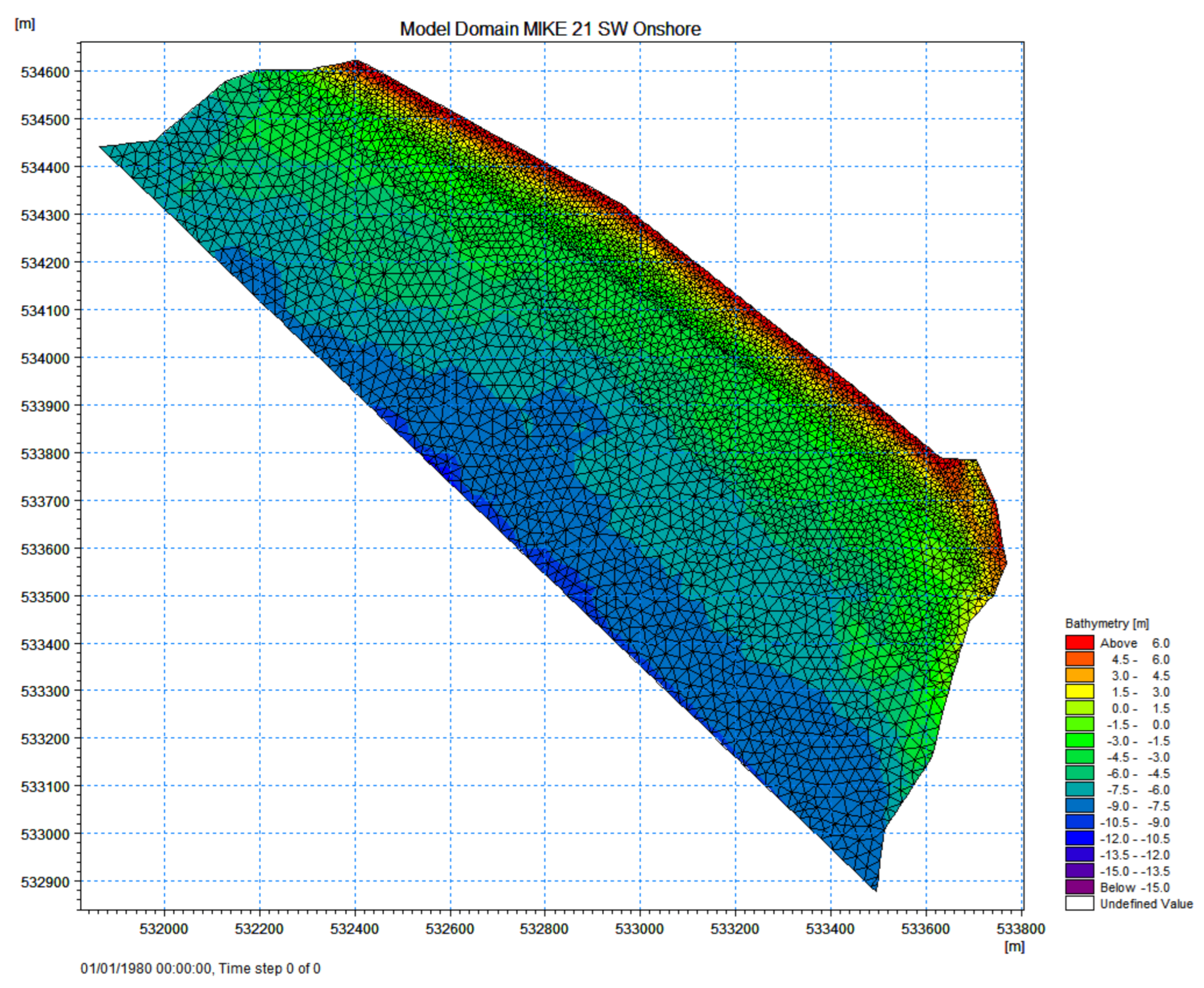
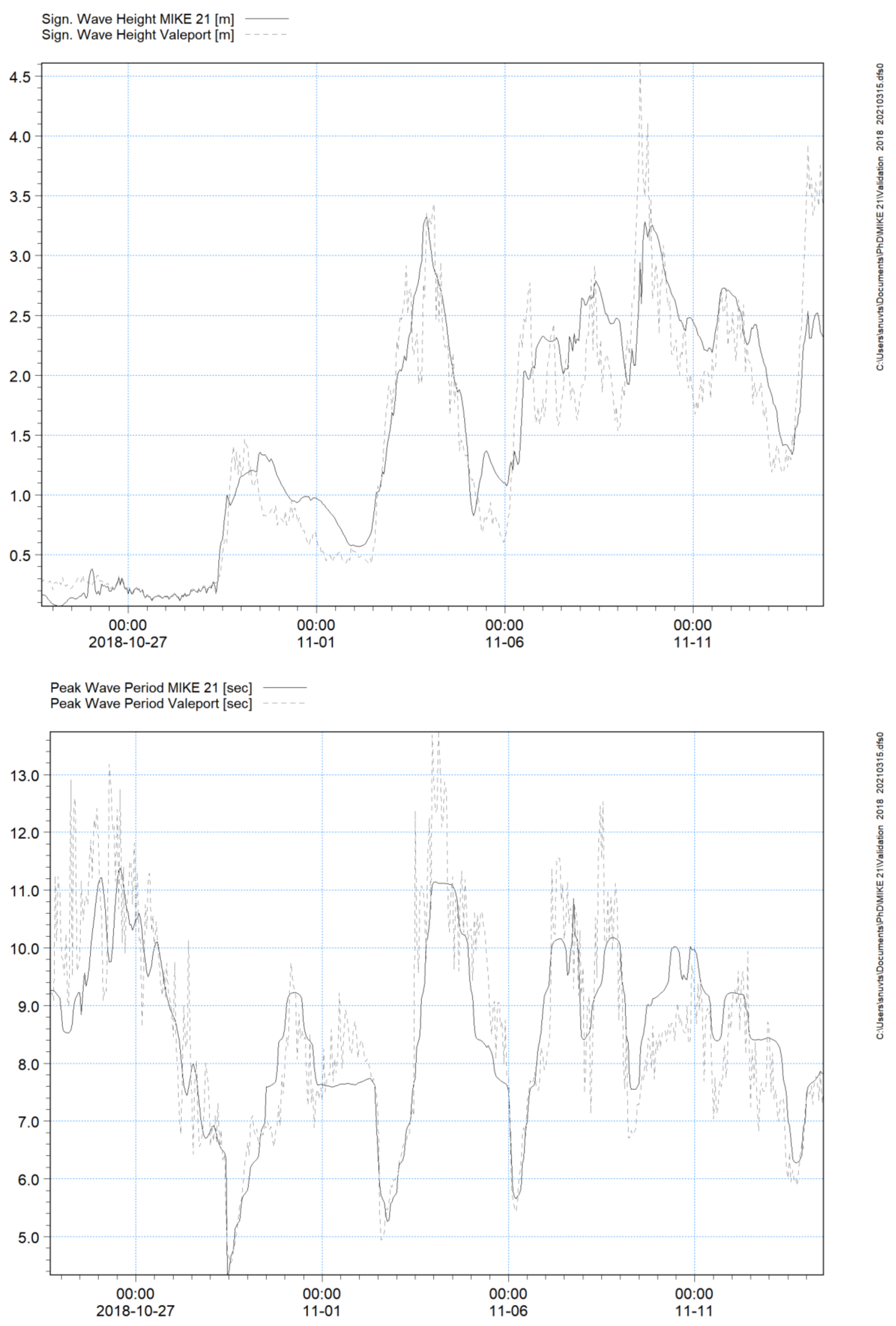
3.2. Hydrodynamics
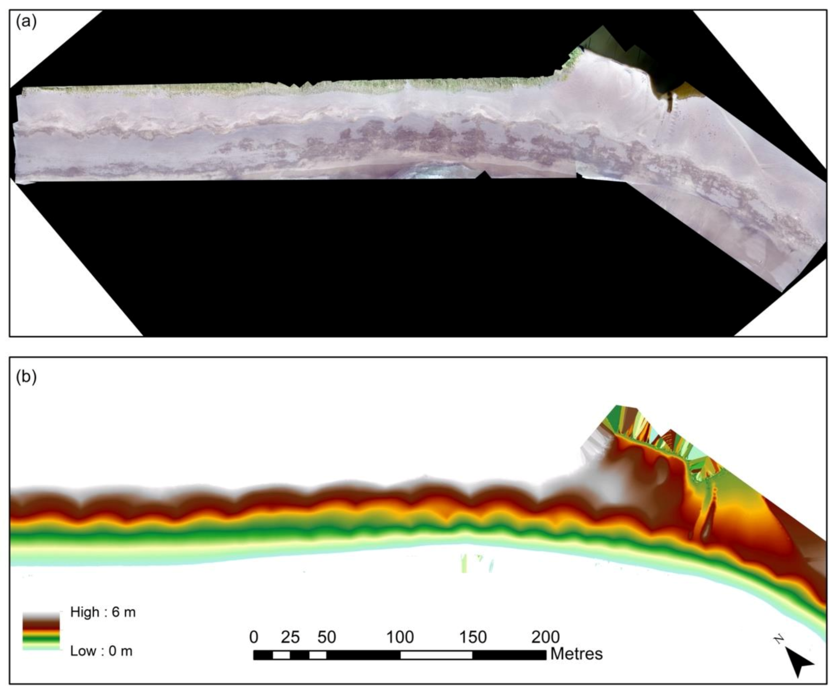
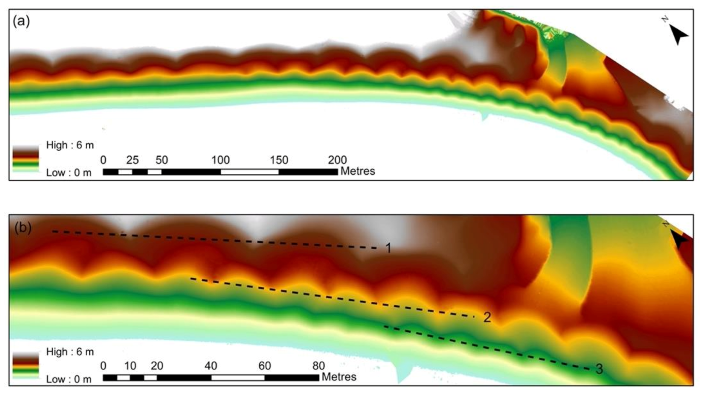
3.3. UAV Survey Method
4. Results
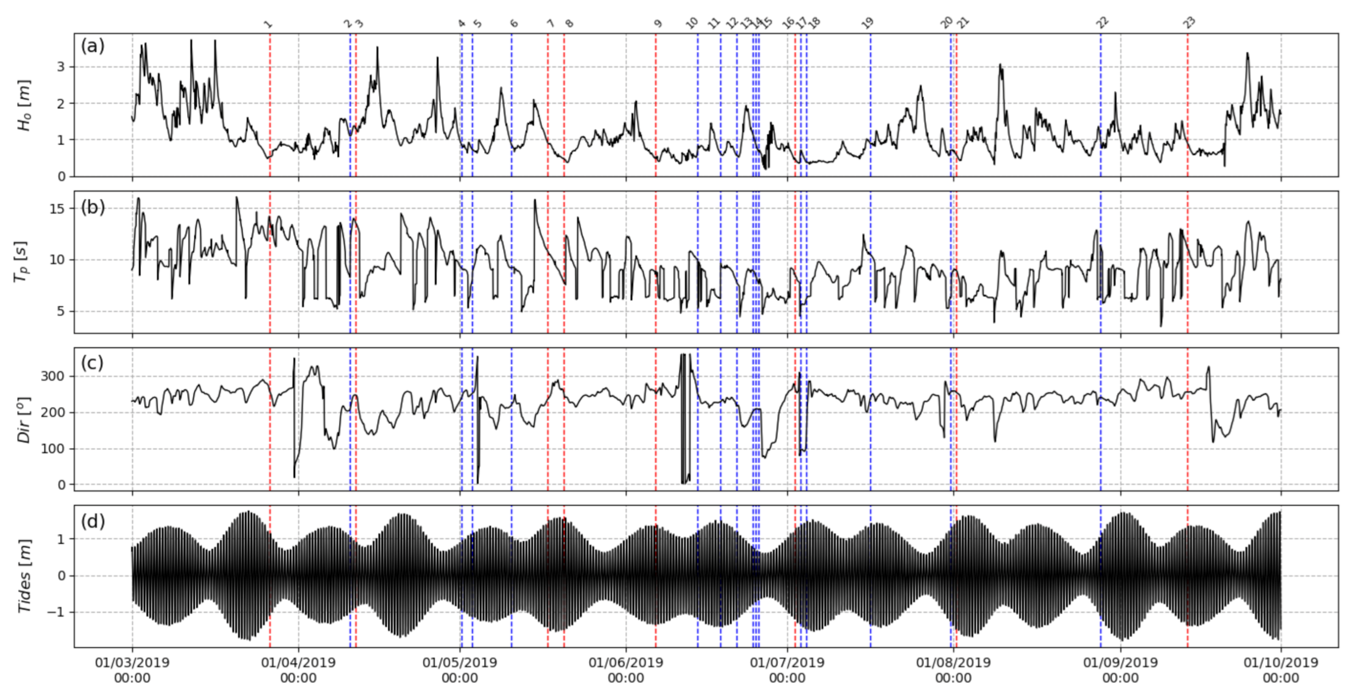
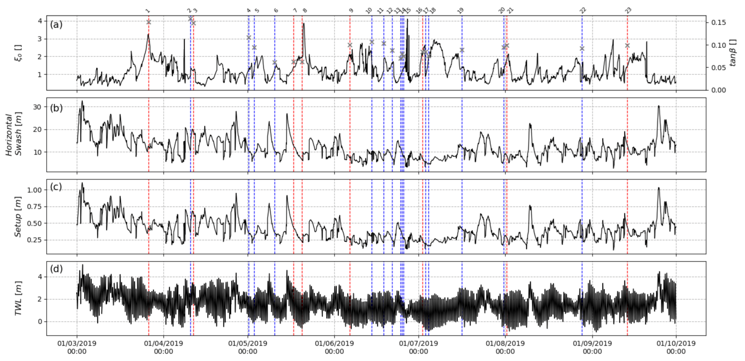
4.1. Hydrodynamics
4.2. Cusp Parameters
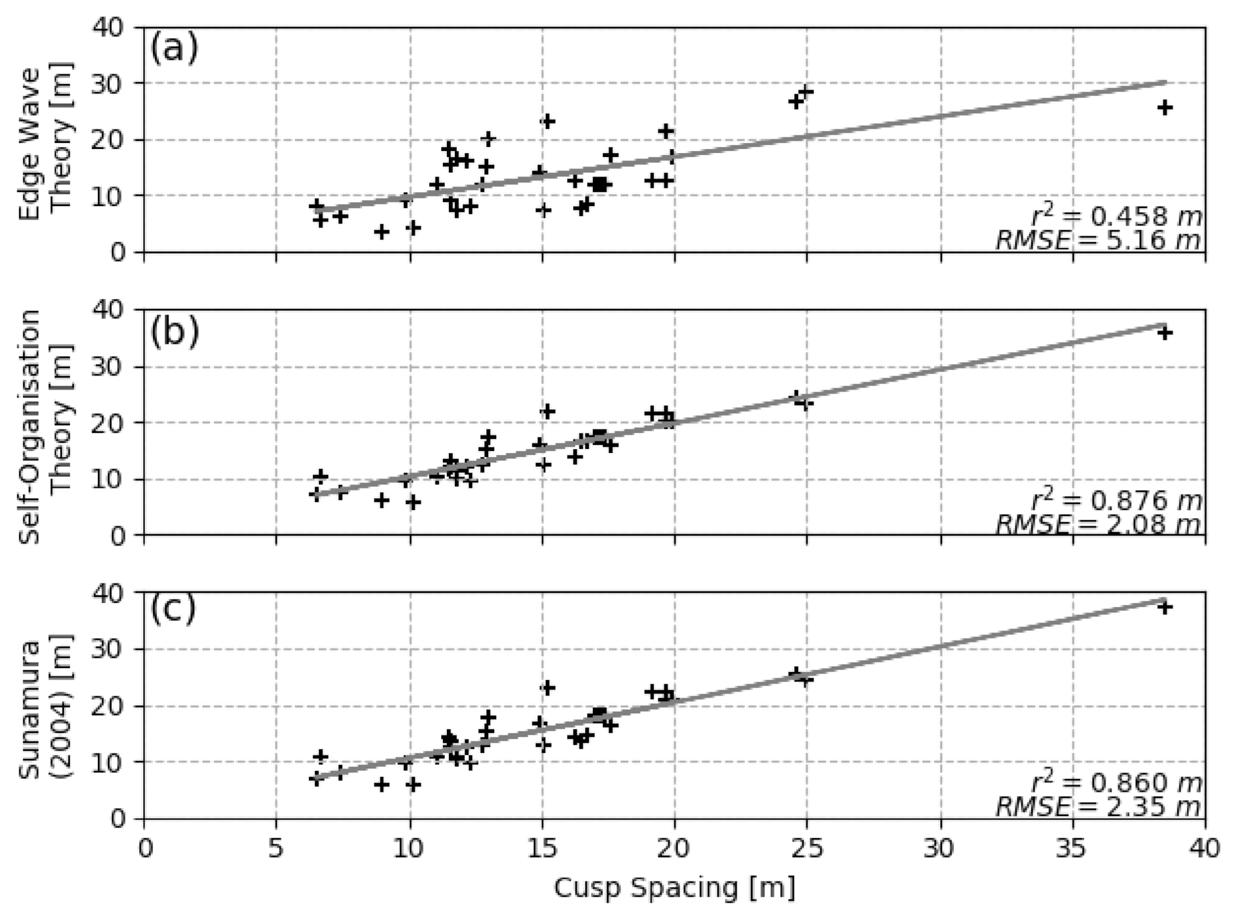
4.3. Beach Cusp Predictions
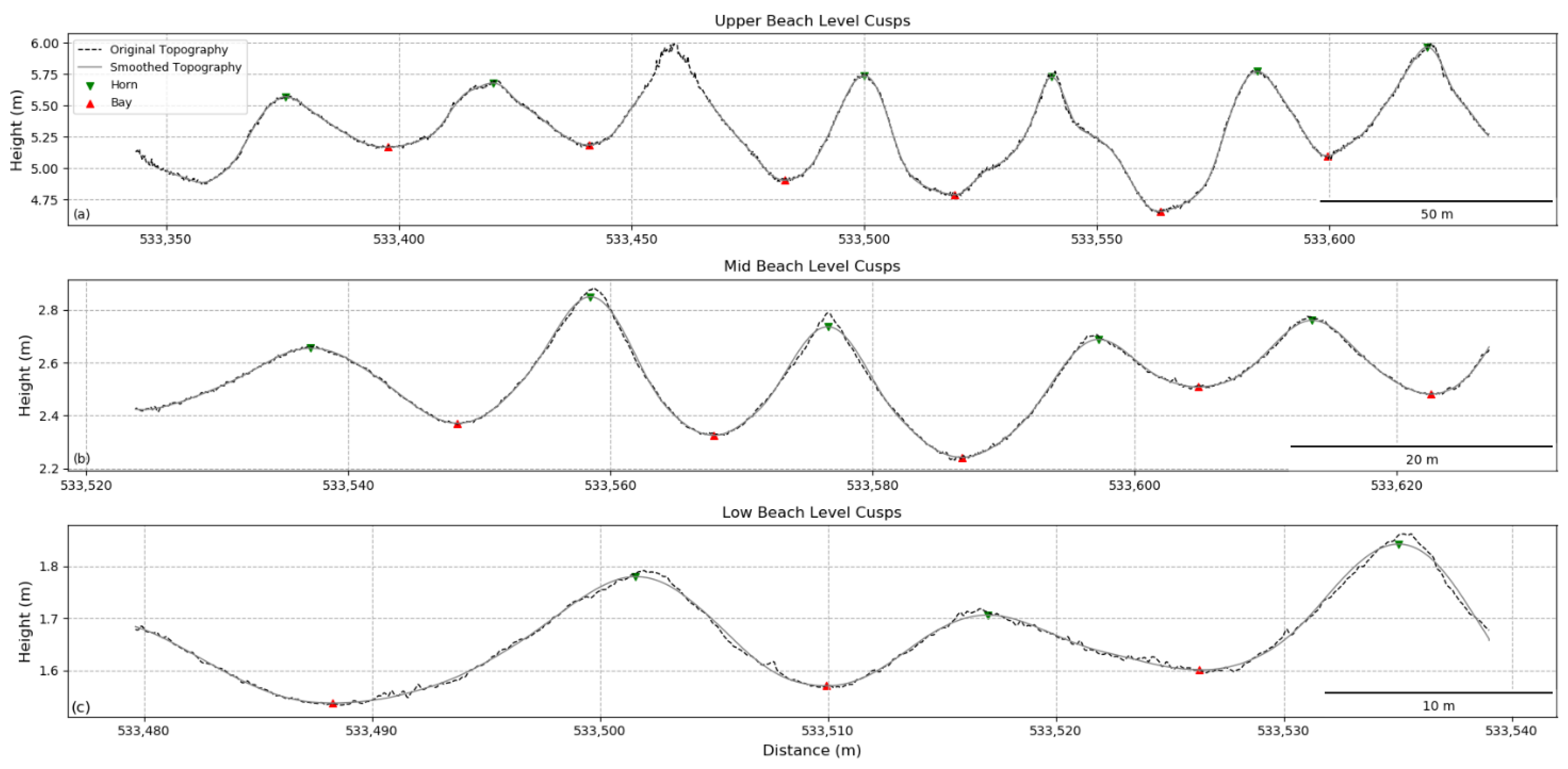
4.3.1. Lower Beach Level Cusps
4.3.2. Mid Beach Level Cusps
4.3.3. Upper Beach Level Cusps
4.4. Prediction Theory Cusp Parameters
5. Discussion
5.1. Cusp Parameters
5.2. Beach Cusp Predictions
5.3. Multilevel Beach Cusp System
6. Conclusions
Author Contributions
Funding
Institutional Review Board Statement
Informed Consent Statement
Data Availability Statement
Acknowledgments
Conflicts of Interest
References
- Elfrink, B.; Baldock, T. Hydrodynamics and sediment transport in the swash zone: A review and perspectives. Coast. Eng. 2002, 45, 149–167. [Google Scholar] [CrossRef]
- Masselink, G.; Russell, P. Field measurements of flow velocities on a dissipative and reflective beach? Implications for swash sediment transport. Coast. Dyn. 2006, 1–13. [Google Scholar] [CrossRef]
- Aagaard, T.; Hughes, M.G. Sediment suspension and turbulence in the swash zone of dissipative beaches. Mar. Geol. 2006, 228, 117–135. [Google Scholar] [CrossRef]
- Coco, G.; Murray, A.B. Patterns in the sand: From forcing templates to self-organization. Geomorphology 2007, 91, 271–290. [Google Scholar] [CrossRef]
- Dean, R.G.; Maurmeyer, E.M. Beach cusps at point reyes and drakes bay beaches, California. In Proceedings of the Coastal Engineering 1980, Sydney, Australia, 23–28 March 1980; pp. 863–884. [Google Scholar] [CrossRef]
- Masselink, G.; Hegge, B.J.; Pattiaratchi, C.B. Beach cusp morphodynamics. Earth Surf. Process. Landf. 1997, 22, 1139–1155. [Google Scholar] [CrossRef]
- Masselink, G.; Pattiaratchi, C.B. Morphological evolution of beach cusps and associated swash circulation patterns. Mar. Geol. 1998, 146, 93–113. [Google Scholar] [CrossRef]
- Dodd, N.; Stoker, A.M.; Calvete, D.; Sriariyawat, A. On beach cusp formation. J. Fluid Mech. 2008, 597, 145–169. [Google Scholar] [CrossRef]
- Sallenger, J.A.H. Inverse grading and hydraulic equivalence in grain-flow deposits. J. Sediment. Res. 1979, 49, 553–562. [Google Scholar] [CrossRef]
- Holland, K.; Holman, R. Field observations of beach cusps and swash motions. Mar. Geol. 1996, 134, 77–93. [Google Scholar] [CrossRef]
- Holland, K.T. Beach cusp formation and spacings at Duck, USA. Cont. Shelf Res. 1998, 18, 1081–1098. [Google Scholar] [CrossRef]
- Coco, G.; Huntley, D.A.; O’Hare, T.J. Investigation of a self-organization model for beach cusp formation and development. J. Geophys. Res. Ocean. 2000, 105, 21991–22002. [Google Scholar] [CrossRef]
- Masselink, G. Alongshore variation in beach cusp morphology in a coastal embayment. Earth Surf. Process. Landf. 1999, 24, 335–347. [Google Scholar] [CrossRef]
- Aoki, H.; Sunamura, T. A laboratory experiment on the formation and morphology of beach cusps. Chikei 2000, 21, 291–306. [Google Scholar]
- Pais-Barbosa, J.; Veloso-Gomes, F.; Taveira-Pinto, F. Coastal features in the energetic and mesotidal West Coast of Portugal. J. Coast. Res. 2007, 50, 459–463. [Google Scholar]
- Bowen, A.J.; Bowen, A. Edge Waves and the littoral environment. In Proceedings of the 13th International Conference on Coastal Engineering, Vancouver, BC, Canada, 10–14 July 1972. [Google Scholar] [CrossRef]
- Guza, R.T.; Inman, D.L. Edge waves and beach cusps. J. Geophys. Res. Atmos. 1975, 80, 2997–3012. [Google Scholar] [CrossRef]
- Kaneko, A. Formation of beach cusps in a wave tank. Coast. Eng. 1985, 9, 81–98. [Google Scholar] [CrossRef]
- Seymour, R.J.; Aubrey, D.G. Rhythmic beach cusp formation: A conceptual synthesis. Mar. Geol. 1985, 65, 289–304. [Google Scholar] [CrossRef]
- Sherman, D.J.; Orford, J.D.; Carter, R.W.G. Development of cusp-related, gravel size and shape facies at Malin Head, Ireland. Sedimentology 1993, 40, 1139–1152. [Google Scholar] [CrossRef]
- Ciriano, Y.; Coco, G.; Bryan, K.R.; Elgar, S. Field observations of swash zone infragravity motions and beach cusp evolution. J. Geophys. Res. Ocean. 2005, 110. [Google Scholar] [CrossRef]
- Werner, B.T.; Fink, T.M. Beach cusps as self-organized patterns. Science 1993, 260, 968–971. [Google Scholar] [CrossRef]
- Coco, G.; O’Hare, T.J.; Huntley, D.A. Beach cusps: A comparison of data and theories for their formation. J. Coast. Res. 1999, 15, 741–749. [Google Scholar]
- Sunamura, T. A predictive relationship for the spacing of beach cusps in nature. Coast. Eng. 2004, 51, 697–711. [Google Scholar] [CrossRef]
- Antia, E. Preliminary field observations on beach cusp formation and characteristics on tidally and morphodynamically distinct beaches on the Nigerian coast. Mar. Geol. 1987, 78, 23–33. [Google Scholar] [CrossRef]
- Carter, R.W.G.; Orford, J.D. The morphodynamics of coarse clastic beaches and barriers: A short- and long-term perspective. J. Coast. Res. 1993, 15, 158–179. [Google Scholar]
- Vousdoukas, M. Erosion/accretion patterns and multiple beach cusp systems on a meso-tidal, steeply-sloping beach. Geomorphology 2012, 141–142, 34–46. [Google Scholar] [CrossRef]
- Almar, R.; Coco, G.; Bryan, K.R.; Huntley, D.; Short, A.; Senechal, N. Video observations of beach cusp morphodynamics. Mar. Geol. 2008, 254, 216–223. [Google Scholar] [CrossRef]
- Almar, R.; Hounkonnou, N.; Anthony, E.J.; Castelle, B.; Senechal, N.; Laibi, R.; Mensah-Senoo, T.; Degbe, G.; Quenum, M.; Dorel, M.; et al. The Grand Popo beach 2013 experiment, Benin, West Africa: From short timescale processes to their integrated impact over long-term coastal evolution. J. Coast. Res. 2014, 70, 651–656. [Google Scholar] [CrossRef]
- Sénéchal, N.; Laibi, R.; Almar, R.; Castelle, B.; Biausque, M.; Lefebvre, J.-P.; Anthony, E.J.; Dorel, M.; Chuchla, R.; Hounkonnou, M.; et al. Observed destruction of a beach cusp system in presence of a double-coupled cusp system: The example of Grand Popo, Benin. J. Coast. Res. 2014, 70, 669–674. [Google Scholar] [CrossRef]
- Angnuureng, D.B.; Bonou, F.; Sohou, Z.; Almar, R.; Alory, G.; Du Penhoat, Y. Shoreline and beach cusps dynamics at the low tide terraced grand Popo Beach, Bénin (West Africa): A statistical approach. J. Coast. Res. 2018, 81, 138–144. [Google Scholar] [CrossRef]
- Nolan, T.; Kirk, R.; Shulmeister, J. Beach cusp morphology on sand and mixed sand and gravel beaches, South Island, New Zealand. Mar. Geol. 1999, 157, 185–198. [Google Scholar] [CrossRef]
- Van Gaalen, J.F.; Kruse, S.E.; Coco, G.; Collins, L.; Doering, T. Observations of beach cusp evolution at Melbourne Beach, Florida, USA. Geomorphology 2011, 129, 131–140. [Google Scholar] [CrossRef]
- Blott, S.J.; Pye, K. Particle shape: A review and new methods of characterization and classification. Sedimentology 2008, 55, 31–63. [Google Scholar] [CrossRef]
- Bosom, E.; Jiménez, J.A. Probabilistic coastal vulnerability assessment to storms at regional scale—Application to Catalan beaches (NW Mediterranean). Nat. Hazards Earth Syst. Sci. 2011, 11, 475–484. [Google Scholar] [CrossRef]
- Stockdon, H.F.; Sallenger, A.H.; Holman, R.A.; Howd, P.A. A simple model for the spatially-variable coastal response to hurricanes. Mar. Geol. 2007, 238, 1–20. [Google Scholar] [CrossRef]
- Serafin, K.A.; Ruggiero, P.; Stockdon, H.F. The relative contribution of waves, tides, and non-tidal residuals to extreme total water levels on US West Coast sandy beaches. Geophys. Res. Lett. 2017, 44, 1839–1847. [Google Scholar] [CrossRef]
- Guza, R.T.; Thornton, E.B. Swash oscillations on a natural beach. J. Geophys. Res. Ocean. 1982, 87, 483–491. [Google Scholar] [CrossRef]
- Holman, R.A.; Sallenger, A.H. Setup and swash on a natural beach. J. Geophys. Res. Space Phys. 1985, 90, 945. [Google Scholar] [CrossRef]
- Holman, R. Extreme value statistics for wave run-up on a natural beach. Coast. Eng. 1986, 9, 527–544. [Google Scholar] [CrossRef]
- Ruessink, B.G.; Kleinhans, M.G.; van de Beukel, P.G.L. Observations of swash under highly dissipative conditions. J. Geophys. Res. Ocean. 1998, 103, 3111–3118. [Google Scholar] [CrossRef]
- Passarella, M.; De Muro, S.; Ruju, A.; Coco, G. An assessment of swash excursion predictors using field observations. J. Coast. Res. 2018, 85, 1036–1040. [Google Scholar] [CrossRef]
- Vousdoukas, M.; Velegrakis, A.; Dimou, K.; Zervakis, V.; Conley, D. Wave run-up observations in microtidal, sediment-starved pocket beaches of the Eastern Mediterranean. J. Mar. Syst. 2009, 78, S37–S47. [Google Scholar] [CrossRef]
- Ferguson, R.; Church, M. A simple universal equation for grain settling velocity. J. Sediment. Res. 2004, 74, 933–937. [Google Scholar] [CrossRef]
- Wright, L.; Short, A. Morphodynamic variability of surf zones and beaches: A synthesis. Mar. Geol. 1984, 56, 93–118. [Google Scholar] [CrossRef]
- Nuyts, S.; Murphy, J.; Li, Z.; Hickey, K. A methodology to assess the morphological change of a multilevel beach cusp system and their hydrodynamics: Case study of Long Strand, Ireland. J. Coast. Res. 2020, 95, 593–598. [Google Scholar] [CrossRef]
- Garnier, R.; Sánchez, M.O.; Losada, M.Á.; Falqués, A.; Dodd, N. Beach cusps and inner surf zone processes: Growth or destruction? A case study of Trafalgar Beach (Cádiz, Spain). Sci. Mar. 2010, 74, 539–553. [Google Scholar] [CrossRef]
- Takeda, I.; Sunamura, T. Formation and Spacing of Beach Cusps. Coast. Eng. Jpn. 1983, 26, 121–135. [Google Scholar] [CrossRef]
- O’Dea, A.; Brodie, K.L. Spectral analysis of beach cusp evolution using 3D lidar scans. Coast. Sediments 2019, 657–673. [Google Scholar] [CrossRef]
- Qi, H.; Cai, F.; Lei, G.; Cao, H.; Shi, F. The response of three main beach types to tropical storms in South China. Mar. Geol. 2010, 275, 244–254. [Google Scholar] [CrossRef]
- Van Enckevort, I.M.J.; Turner, I.L.; Plant, N.; Holman, R.A.; Ruessink, B.G.; Coco, G.; Suzuki, K. Observations of nearshore crescentic sandbars. J. Geophys. Res. Ocean. 2004, 109. [Google Scholar] [CrossRef]
- Coco, G.; Burnet, T.K.; Werner, B.T.; Elgar, S. Test of self-organization in beach cusp formation. J. Geophys. Res. Atmos. 2003, 108. [Google Scholar] [CrossRef]
- Castelle, B.; Ruessink, B.G.; Bonneton, P.; Marieu, V.; Bruneau, N.; Price, T.D. Coupling mechanisms in double sandbar systems. Part 1: Patterns and physical explanation. Earth Surf. Process. Landf. 2010, 35, 476–486. [Google Scholar] [CrossRef]


| Sampling Setup 730D Valeport | ||
|---|---|---|
| Parameter | Value | Unit |
| Rate | 1 | Hz |
| Tide Burst Duration | 20 | Seconds |
| Tide Burst Interval | 60 | Minutes |
| Wave Burst Duration | 1024 | Samples |
| Wave Burst Interval | 60 | Minutes |
| Statistical Parameters Model Validation | |||
|---|---|---|---|
| Wave Parameter | R | RMSE | Bias |
| Hs | 0.919 | 0.401 | 0.081 |
| Tp | 0.840 | 1.005 | 0.129 |
| Overview Cusp Parameters | ||||||
|---|---|---|---|---|---|---|
| Date | Level | Cusp Spacing (m) | Cusp Amplitude (m) | Cusp Elevation (m) | Cusp Depth (m) | |
| 1 | 26 March | Upper Beach | 39.9 | 0.86 | 5.41 | 16.91 |
| Mid Beach | 38.5 | 0.58 | 3.14 | 16.57 | ||
| Low Beach | - | |||||
| 2 | 10 April | Upper Beach | 40.3 | 0.83 | 5.46 | 15.01 |
| Mid Beach | 24.6 | 0.34 | 2.81 | 12.31 | ||
| Low Beach | 11.5 | 0.25 | 1.91 | 9.87 | ||
| 3 | 11 April | Upper Beach | 39.2 | 0.87 | 5.62 | 14.98 |
| Mid Beach | 25.0 | 0.43 | 2.76 | 12.69 | ||
| Low Beach | - | |||||
| 4 | 01 May | Upper Beach | 38.9 | 1.05 | 4.87 | 15.67 |
| Mid Beach | 14.9 | 0.21 | 2.33 | 9.06 | ||
| Low Beach | 11.6 | 0.32 | 2.08 | 6.01 | ||
| 5 | 03 May | Upper Beach | 37.7 | 0.81 | 5.69 | 13.24 |
| Mid Beach | 12.8 | 0.23 | 2.42 | 8.81 | ||
| Low Beach | 12.3 | 0.04 | 1.03 | 2.73 | ||
| 6 | 10 May | Upper Beach | 37.9 | 0.79 | 5.68 | 12.32 |
| Mid Beach | 19.9 | 0.29 | 2.96 | 8.55 | ||
| Low Beach | 16.5 | 0.18 | 1.82 | 8.97 | ||
| 7 | 17 May | Upper Beach | 40.9 | 0.86 | 5.71 | 15.94 |
| Mid Beach | 19.7 | 0.36 | 3.01 | 8.48 | ||
| Low Beach | - | |||||
| 8 | 20 May | Upper Beach | 40.9 | 0.86 | 5.72 | 15.40 |
| Mid Beach | 19.7 | 0.42 | 2.99 | 8.62 | ||
| Low Beach | - | |||||
| 9 | 06 June | Upper Beach | 40.8 | 0.86 | 5.73 | 15.39 |
| Mid Beach | 11.1 | 0.22 | 2.68 | 15.14 | ||
| Low Beach | - | |||||
| 10 | 14 June | Upper Beach | 40.9 | 0.84 | 5.72 | 15.02 |
| Mid Beach | 12.2 | 0.71 | 3.47 | 15.42 | ||
| Low Beach | 11.8 | 0.13 | 1.15 | 5.39 | ||
| 11 | 18 June | Upper Beach | 40.2 | 0.84 | 5.81 | 15.47 |
| Mid Beach | 15.1 | 0.31 | 3.04 | 8.06 | ||
| Low Beach | 7.4 | 0.15 | 2.14 | 7.54 | ||
| 12 | 21 June | Upper Beach | 40.9 | 0.85 | 5.74 | 15.53 |
| Mid Beach | 16.3 | 0.39 | 2.64 | 8.35 | ||
| Low Beach | 9.9 | 0.09 | 1.41 | 11.61 | ||
| 13 | 24 June | Upper Beach | 40.9 | 0.84 | 5.68 | 15.35 |
| Mid Beach | 17.0 | 0.40 | 2.51 | 11.43 | ||
| Low Beach | 16.7 | 0.22 | 1.71 | 7.39 | ||
| 14 | 25 June | Upper Beach | 40.8 | 0.83 | 5.74 | 17.21 |
| Mid Beach | 17.1 | 0.42 | 2.73 | 11.36 | ||
| Low Beach | 11.6 | 0.14 | 1.62 | 4.75 | ||
| 15 | 25 June | Upper Beach | 40.8 | 0.83 | 5.67 | 17.25 |
| Mid Beach | 17.2 | 0.44 | 2.57 | 11.49 | ||
| Low Beach | 11.8 | 0.16 | 1.73 | 4.50 | ||
| 16 | 02 July | Upper Beach | 40.8 | 0.84 | 5.71 | 14.93 |
| Mid Beach | 17.4 | 0.47 | 2.68 | 10.60 | ||
| Low Beach | - | |||||
| 17 | 03 July | Upper Beach | 40.8 | 0.85 | 5.69 | 15.35 |
| Mid Beach | 17.3 | 0.48 | 2.68 | 10.85 | ||
| Low Beach | 6.5 | 0.18 | 1.84 | 6.96 | ||
| 18 | 04 July | Upper Beach | 40.9 | 0.83 | 5.69 | 15.06 |
| Mid Beach | 17.4 | 0.47 | 2.64 | 10.71 | ||
| Low Beach | 9.0 | 0.30 | 1.86 | 5.01 | ||
| 19 | 16 July | Upper Beach | 40.8 | 0.85 | 5.71 | 15.21 |
| Mid Beach | 17.6 | 0.42 | 2.74 | 10.73 | ||
| Low Beach | 12.9 | 0.15 | 1.92 | 7.48 | ||
| 20 | 31 July | Upper Beach | 40.7 | 0.85 | 5.80 | 15.36 |
| Mid Beach | 19.2 | 0.32 | 2.6 | 11.04 | ||
| Low Beach | 10.2 | 0.07 | 1.11 | 2.0 | ||
| 21 | 01 Aug | Upper Beach | 40.8 | 0.85 | 5.79 | 15.41 |
| Mid Beach | 19.7 | 0.30 | 2.57 | 10.22 | ||
| Low Beach | - | |||||
| 22 | 28 Aug | Upper Beach | 39.4 | 0.78 | 5.61 | 16.39 |
| Mid Beach | 15.2 | 0.55 | 3.06 | 7.68 | ||
| Low Beach | 6.7 | 0.18 | 1.21 | 7.66 | ||
| 23 | 13 Sept | Upper Beach | 40.8 | 0.85 | 5.73 | 15.37 |
| Mid Beach | 13.0 | 0.33 | 3.03 | 8.50 | ||
| Low Beach | - | |||||
| Statistical Analysis Cusp Spacing | |||
|---|---|---|---|
| Mean (m) | Standard Deviation (m) | Coefficient of Variation | |
| Upper beach level | 40.26 | 0.95 | 0.02 |
| Mid beach level | 18.17 | 5.48 | 0.30 |
| Low beach level | 11.09 | 2.91 | 0.26 |
| Performance Cusp Spacing Predictions | ||||
|---|---|---|---|---|
| Theory | RMSE (m) | r2 | Equation | Fitting Coefficient |
| Edge-Wave Theory | 4.78 | 0.087 | m = 0.4845 | |
| Self-Organisation Theory | 2.03 | 0.642 | f = 1.1628 | |
| Sunamura (2004) | 2.37 | 0.473 | A = 0.7032 | |
| Resulting Hydrodynamics for Mid Beach Level Cusps | ||||
|---|---|---|---|---|
| Survey | Date | Observed Cusp Spacing (m) | Predicted Self Organisation (m) | Occurrence |
| 1 | 26 March | 38.48 | 37.81 | 03/03/2019T00:00 |
| 2 | 10 April | 24.64 | 22.90 | 09/04/2019T04:00 |
| 3 | 11 April | 25.05 | 23.22 | 11/04/2019T08:00 |
| 4 | 01 May | 14.97 | 14.97 | 30/04/2019T18:00 |
| 5 | 03 May | 12.84 | 12.27 | 01/05/2019T08:00 |
| 6 | 10 May | 19.90 | 20.04 | 09/05/2019T10:00 |
| 7 | 17 May | 19.71 | 19.63 | 16/05/2019T10:00 |
| 8 | 20 May | 19.68 | 19.63 | 16/05/2019T10:00 |
| 9 | 06 June | 11.15 | 11.89 | 04/06/2019T06:00 |
| 10 | 14 June | 11.19 | 11.24 | 13/06/2019T14:00 |
| 11 | 18 June | 15.07 | 12.03 | 16/06/2019T22:00 |
| 12 | 21 June | 16.31 | 12.85 | 19/06/2019T22:00 |
| 13 | 24 June | 17.05 | 17.45 | 23/06/2019T18:00 |
| 14 | 25 June | 17.12 | 17.45 | 23/06/2019T18:00 |
| 15 | 25 June | 17.15 | 17.45 | 23/06/2019T18:00 |
| 16 | 02 July | 17.37 | 17.45 | 23/06/2019T18:00 |
| 17 | 03 July | 17.31 | 17.45 | 23/06/2019T18:00 |
| 18 | 04 July | 17.39 | 17.45 | 23/06/2019T18:00 |
| 19 | 16 July | 17.55 | 15.63 | 15/07/2019T20:00 |
| 20 | 31 July | 19.23 | 20.74 | 25/07/2019T22:00 |
| 21 | 01 Aug | 19.65 | 20.74 | 25/07/2019T22:00 |
| 22 | 28 Aug | 15.19 | 18.91 | 27/08/2019T19:00 |
| 23 | 13 Sept | 13.01 | 16.79 | 13/09/2019T05:00 |
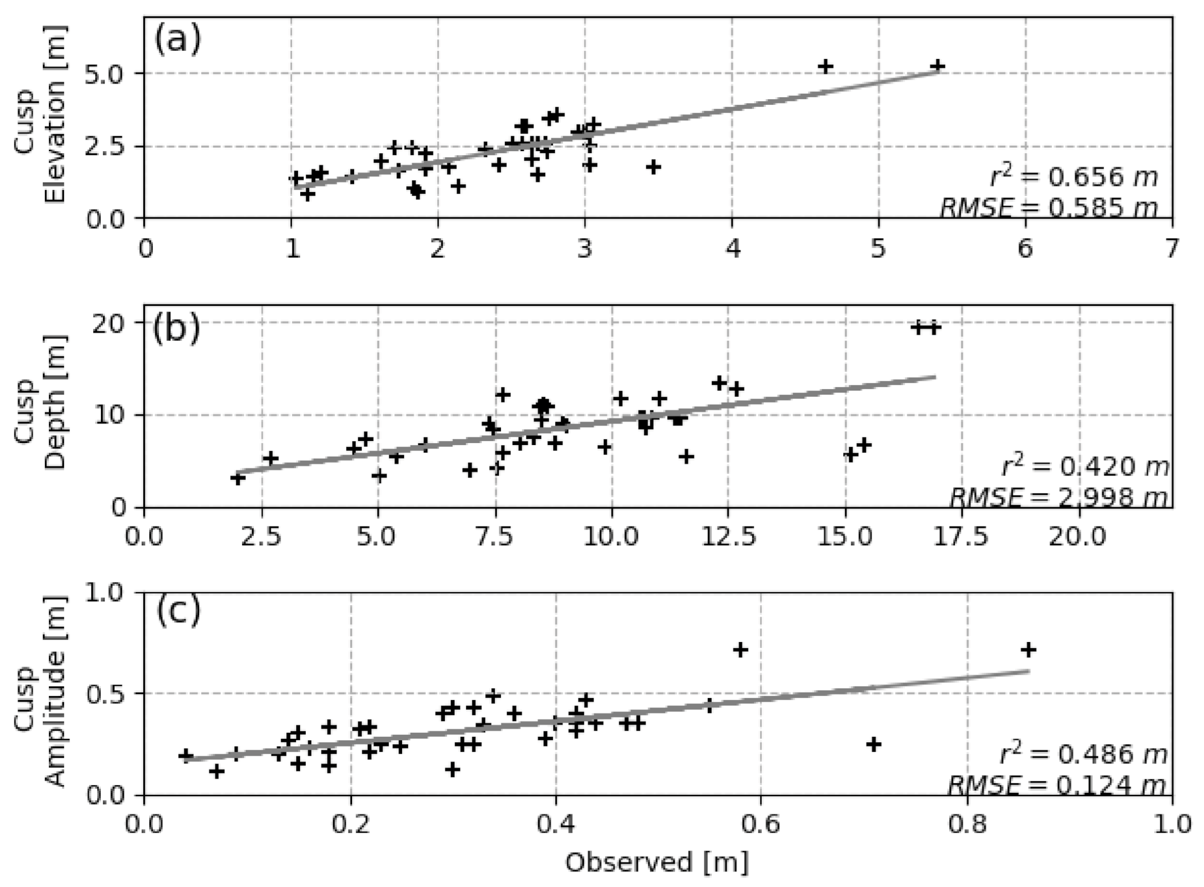
| Prediction Cusp Parameters | ||||
|---|---|---|---|---|
| Parameter | Equation | Fitting Coefficient | RMSE (m) | R |
| Cusp Elevation | ne = 0.171 | 0.585 | 0.810 | |
| Cusp Depth | nd = 0.636 | 2.998 | 0.648 | |
| Cusp Amplitude | na = 0.023 | 0.124 | 0.697 | |
Publisher’s Note: MDPI stays neutral with regard to jurisdictional claims in published maps and institutional affiliations. |
© 2021 by the authors. Licensee MDPI, Basel, Switzerland. This article is an open access article distributed under the terms and conditions of the Creative Commons Attribution (CC BY) license (http://creativecommons.org/licenses/by/4.0/).
Share and Cite
Nuyts, S.; Li, Z.; Hickey, K.; Murphy, J. Field Observations of a Multilevel Beach Cusp System and Their Swash Zone Dynamics. Geosciences 2021, 11, 148. https://doi.org/10.3390/geosciences11040148
Nuyts S, Li Z, Hickey K, Murphy J. Field Observations of a Multilevel Beach Cusp System and Their Swash Zone Dynamics. Geosciences. 2021; 11(4):148. https://doi.org/10.3390/geosciences11040148
Chicago/Turabian StyleNuyts, Siegmund, Zili Li, Kieran Hickey, and Jimmy Murphy. 2021. "Field Observations of a Multilevel Beach Cusp System and Their Swash Zone Dynamics" Geosciences 11, no. 4: 148. https://doi.org/10.3390/geosciences11040148
APA StyleNuyts, S., Li, Z., Hickey, K., & Murphy, J. (2021). Field Observations of a Multilevel Beach Cusp System and Their Swash Zone Dynamics. Geosciences, 11(4), 148. https://doi.org/10.3390/geosciences11040148