Mass Balance of Austre Grønfjordbreen, Svalbard, 2006–2020, Estimated by Glaciological, Geodetic and Modeling Aproaches

Abstract

Glacier mass balance measurements, reconstructions and modeling are the precondition for assessing glacier sensitivity to regional climatic fluctuations. This paper presents new glaciological and geodetic mass balance data of Austre Grønfjordbreen located in the western part of Nordenskiöld Land in Central Spitsbergen. The average annual mass balance from 2014 to 2019 was −1.59 m w.e. The geodetic mass balance from 2008 to 2017 was −1.34 m w.e. The mass balance was also reconstructed by the temperature-index model from 2006 to 2020 and by spatially-distributed energy-balance models for 2011–2015 and 2019. We found a cumulative mass balance of −21.62 m w.e. over 2006–2020. The calculated mass-balance sensitivity to temperature was −1.04 m w.e. °C⁻¹, which corresponds to the highest glacier mass balance sensitivity among Svalbard glaciers. Sensitivity to precipitation change was 0.10 m w.e. for a 10% increase in precipitation throughout the balance year. Comparing the results of the current study with other glacier mass balance assessments in Svalbard, we found that Austre Grønfjordbreen loses mass most rapidly due to its location, which is mostly influenced by the warm West Spitsbergen Current, small area and low elevation range.

1. Introduction

Glaciers are widely acknowledged as indicators of climate change and are currently among the major contributors to sea level rise [1]. Winter precipitation and summer temperatures both have an influence on the amount of snow accumulated and the amount of snow and ice lost by melting; thus changes in glacier mass are linked to changes in climate [2,3]. According to recent projections, global mass loss of all glaciers outside the Antarctic and Greenland ice sheets by 2100 relative to 2015 averaged over 25 General Circulation Models (GCMs) runs varies from 18 ± 7% (RCP2.6) to 36 ± 11% (RCP8.5) corresponding to 94 ± 25 and 200 ± 44 mm sea-level equivalent (SLE), respectively [4].

The Svalbard archipelago is located in one of the most rapidly warming regions on Earth and undergoes an increase in average summer temperature and duration of melt period along with the impacts of early summer and late autumn rainfalls. For the moderate emission scenario RCP4.5, a warming of 5–8 °C and a precipitation increase of 20–40% is predicted for Svalbard by 2100, relative to the period of 1986–2005. Svalbard glaciers are expected to lose ~50% of their mass by 2100 [5]. Glaciers cover ~57% of the land area of Svalbard [6] and, if melted, could potentially contribute 17 ± 2 mm to global sea-level rise [7].

The direct mass balance measurements of Svalbard glaciers began in 1950 (Finsterwalderbreen) by the Norwegian Polar Institute. In 1966, investigations were started in the Kongsfjord area on Austre Brøggerbreen and, a year later, on Midtre Lovénbreen. Polish researchers have studied the mass balance on Hansbreen in Hornsund (southern Spitsbergen) since 1989. In 1987, mass balance investigations were started on Kongsvegen [8,9]. The longest record of field mass balance measurements in Svalbard exists for two small glaciers, Austre Brøggerbreen and Midtre Lovénbreen, where the measurements began in the mid-1960s [10]. At present, there are 13 glaciers with continuous annual mass balance records longer than 5 years, mostly located along the western coast in the Kongsfjord area [10,11]. A number of regional glacier change and mass balance modeling studies show high spatial variability of glacier mass changes within the archipelago with the highest rates of mass losses in the southern parts [10], and specifically in Nordenskiöld Land [12].

In this study, we focuses on Austre Grønfjordbreen located in Nordenskiöld Land. The in situ measurements in Nordenskiöld Land are scarce and not well represented in the regional analysis, which can lead to some underestimation of mass loss in regional mass balance assessments. The Grønfjordbreen system mass balance monitoring (assuming that Austre Grønfjordbreen and Vestre Grønfjordbreen form its entire area) started in 1966. The first published balance data for Vestre Grønfjordbreen go back to 1965/66 and 1966/67. Later, in 1985/86 and 1986/87, mass balance was measured on both Austre and Vestre Grønfjordbreen [13]. Mass balance measurements on Austre Grønfjordbreen were started in 2004 [14,15]. However, observations included a limited number of ablation stakes, and until 2013, the mass balance data were inconsistent and randomly reported. Since 2013, the observations were re-established on Austre Grønfjordbreen and included a new ablation stakes network and high resolution GPR surveys of snow thickness together with traditional snow surveys [16,17].

The main purpose of this study is to present the new data of surface mass balance of Austre Grønfjordbreen and to update previous mass balance assessments [14,15] by the traditional glaciological approach and geodetic method as well as to reconstruct the time series of annual mass balance by two methods. Based on mass-balance measurements and meteorological data, a temperature-index model, together with the accumulation model, was applied to reconstruct the annual mass balance of Austre Grønfjordbreen from 2006 to 2020. The model was also used to assess the mass balance sensitivity to a regional climate fluctuation. The second method is based on more complicated energy-balance modeling that results in mass distributed mass balance. In this study we applied the A-Melt model for several separate years (2011–2015; 2019). The A-Melt model was originally developed by E. Rets for the North Caucasus glaciers [18,19] and successfully adopted for the Ak-Shyirak massif in the Central Tien-Shan as well [20,21].

Recognizing the scarcity of reported mass-balance data on Nordenskiöld Land, this study supplies new mass-balance information, aiming to provide a basis for further monitoring and application of extended mass-balance models.

2. Data and Methods

2.1. Field Measurements and Data

Austre Grønfjordbreen (77°55’ N, 14°20’ E) is located in the western part of Nordenskiold Land in Central Spitsbergen. The glacier extends from 70 to 550 m a.s.l. and in 2017 covered an area of 6.15 km². The glacier is formed by two tributaries merging in the middle part at the level of 300–360 m a.s.l. Chernov et al. [22] reported that from 1936 to 2017, the glacier lost 44% of its area, from 2003 to 2017 it lost 23%, and 27% was lost from 1990 to 2017. The glacier retreated by 3 km from 1936 to 2017 (Figure 1). Since 2003, the terminus retreat averaged 50 m/year. From 2014 to 2017, the glacier retreated by 450 m, and in 2017 a significant part of the terminus was separated from the glacier. Thus, in one year the length of the glacier decreased by 330 m [15].

The mass-balance monitoring program was re-established in 2013 and included an observation network of 6 stakes measured in late summer-early autumn. Observation periods vary considerably from year to year and could not be tied to the end of the hydrological year (end of September). The monitoring network has been improved annually to increase the representativeness of ablation and accumulation measurements (

Table 1. Number of measurement sites and dates of field surveys.

Balance Year	Number of Stake Measurements	Beginning of Survey Period (dd.mm.yyyy)	End of Winter Season (dd.mm.yyyy)	End of Survey Period (dd.mm.yyyy)	Method of Winter Measurements	Number of Snow Pits	Number of Manual Snow Probings
2019	12	24.08.2018	08.04.2019	11.09.2019	Snow pits; manual snow probings; GPR	6	58
2018	11	10.09.2017		24.08.2018
2017	11	06.09.2016		10.09.2017
2016	10	06.08.2015		06.09.2016
2015			12.04.2015		Snow pits; GPR	12
2014	6	22.08.2013	17.04.2014	02.08.2014	Snow pits; manual snow probings; GPR	13	77
2013			21.04.2013		Snow pits; manual snow probings	10	44

).

Net ablation is measured using wooden stakes, drilled into the ice. Point ablation measurements at the stake locations are converted to water equivalent by using an ice density of 900 kg m⁻³. For winter accumulation, we used the data obtained from snow pits measurements in spring 2013–2015 and 2019. Snow probings are taken following the path of observers along the various snow pits with a distance between the measurement points of about 300 m.

Snow accumulation distribution was also estimated by ground-penetrating radar (GPR) surveys using PulseEKKO PRO radar with 500 MHz shielded antennae. The system was deployed on the glacier surface using a snowmobile. The results of GPR and standard manual snow accumulation surveys along with the comparison of the methods are presented in Lavrentiev et al. [17].

The main meteorological parameters (temperature, wind speed, relative humidity, wind direction, gust speed and pressure) were measured at the automatic weather station (AWS) with 1-hour time steps. The AWS installed in 2014 is situated on the frontal moraine close to the glacier at an elevation of 70 m a.s.l. According to the records, the warmest month is July with an average air temperature of 6.5 °C (2014–2018), and the lowest temperatures were detected from February to April with a mean value of −8.9 °C (2014–2018). One additional AWS was installed in the upper zone of the glacier at 450 m a.s.l. and worked from 2014 to 2015. The temperature lapse rate was calculated using AWS data and data from the temperature sensors that are established every year on three elevation levels during summer field surveys.

There are 3-hour temperature and precipitation data available from Barentsburg AWS, located 15 km to the north from Austre Grønfjordbreen. The mean sum of annual precipitation is 765 mm (2005–2019) with the maximum precipitation occurring in September–March with an average of 108 mm (Figure 2).

2.2. Glaciological Method

Net, summer and winter glaciological mass balance was calculated using stakes observations and snow measurements.

The mass balance of the entire glacier is estimated as a sum of weighted mean mass balance values of separate elevation bands. We set the interval of 50 m elevation difference and then calculated a mean mass balance (b_j) for each individual zone using Topo To Raster interpolation in ArcGIS software (Esri, Redlands, CA, USA) (© ESRI). The interpolation then was checked to avoid artefacts caused by the interpolation method. The mass balance value (b_j) is multiplied by the area (A_j) of each zone, summed and then divided by the total glacier area (A_glacier) to obtain the glacier mass balance (B):

$$B={\displaystyle \sum }_{i=1}^n\left(b_j\times A_j\right)/A_{glacier}$$

(1)

The total glacier area (A_glacier) is estimated for each year by available satellite images.

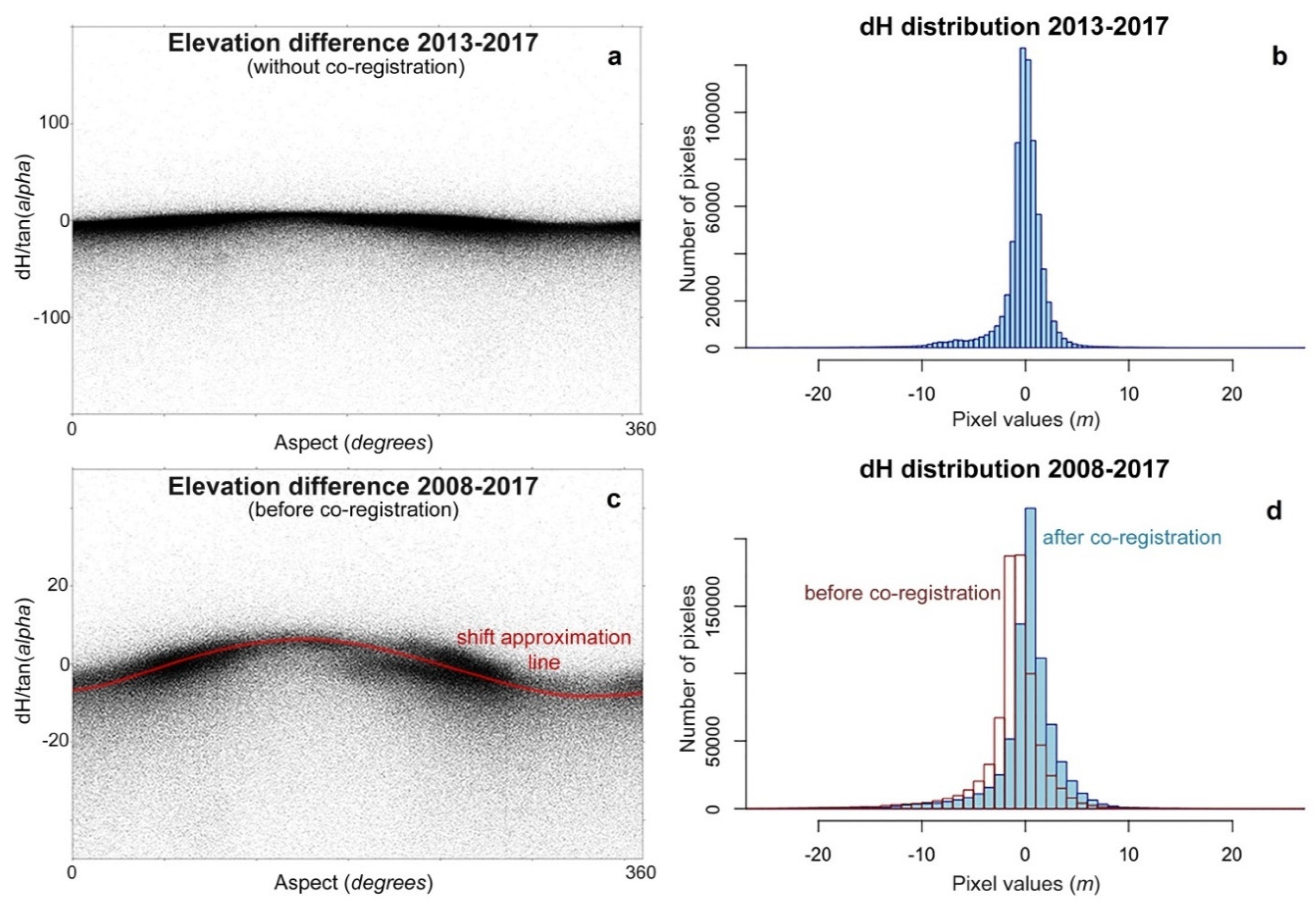
2.3. Geodetic Mass Balance

The geodetic mass balance of Austre Grønfjordbreen was calculated for two periods: 2008–2017 and 2013–2017. The digital elevation models (DEMs) 2008–2017 were co-registered using a procedure suggested by Nuth and Kääb [25], and then DEMS of 2008, 2013 and 2017 were subtracted by pairs (2008–2017 and 2013–2017) to derive the difference in surface elevation for these two periods. The geodetic mass balance for 2008–2013 was calculated after deriving the values for 2013–2017 and 2008–2017.

In this study we used DEMs for three years:

• ArcticDEM v3.0 (©Polar Geospatial Center, University of Minnesota: Minneapolis, MN, USA [26]) of 2 m resolution and dated by 30 June 2017 and 2 August 2017
• ArcticDEM v3.0 of 2 m resolution and dated by 17 August 2013
• DEM 2008 provided by © Norwegian Polar Institute (npolar.no) [27] of 5 m resolution

Elevation change values were obtained for the 2013–2017 and 2008–2017 periods. The geodetic mass balance for 2008–2013 was calculated as a difference between these two values.

The latest ArcticDEM of 2 August 2017 mainly extends to the glacial part of the scene and weakly covers stable topography areas, which are necessary for DEM co-registration. ArcticDEM on 30 June 2017 has more complete coverage of stable relief. The data for 2 August 2017 model cover almost the entire surface within the glacier boundaries of 2013, with insignificant (~50 m) data gaps along the glacier edge. We built a raster mosaic from these layers to get more complete coverage of the glacier surface and stable relief.

To calculate the geodetic mass balance for 2013–2017, both rasters were subtracted (Figure 3a). According to the elevation differences (dH) distribution histogram of 2017 and 2013 DEMs, 97% of the pixels are within ±10 m deviation range (Figure 3b). Larger differences (3% of pixels) are due to rough DEM errors caused by cloudiness and survey errors on steep slopes. The standard deviation (σ) for a stable relief is ±2 m (sample variance is 4.1 m, which is σ squared); 91% of pixels are in the 2σ interval, 80% are in the 1σ interval. For calculation of average values by elevation zones and over the flat surface where a normal distribution of deviations is minimized, the error in the elevation difference can be considered as negligible.

To calculate the geodetic mass balance for 2008–2017, both rasters first were resampled to 10 m resolution, aligned and subtracted (Figure 3c); 96% of dH pixels are in the range of ±10 m, which is caused by rough DEM errors (Figure 3d). After co-registration, σ for a stable relief with the slope >20° is ± 2.5 m. For the stable relief where the slope <20°, which is close to glacier steepness, σ decreases to ±1.9 m; 90% of pixels are in 2σ interval and 74% are in 1σ interval. As in the previous case, the error of the elevation difference of average values by elevation zones on the flat glacial surface is considered as negligible.

2.4. Temperature-Index Modeling

Temperature was found to be one of the main drivers of ice/snow ablation. A simple degree-day model is widely used to determine ablation sensitivity to climate parameters [28,29]. It is assumed that the relationship between melt and temperature is linear for every elevation band. This approach simulates snow and ice surface melt from the sum of positive degree-days (PDD is the sum of daily mean temperatures above the melting point over a given period of time) and melt coefficients for ice and snow (DDF_i and DDF_s, respectively, in mm °C^–1 d^–1).

Here we applied a degree-day model together with an accumulation model to calculate mass balance. Ablation is related to the positive degree-day sum and accumulation is estimated from the sum of solid precipitation. Snow accumulation at any particular altitude is estimated by assuming that precipitation is split between rain and snow near the threshold temperature (1 °C). Rain and meltwater are assumed to run off the glacier and not to contribute to the mass balance. Accumulation is the most inaccurate value due to the fact that distribution of snow on the glacier can be complex and not directly dependent on the amount of precipitation. Therefore, the coefficient C_prec was adopted until the difference between winter precipitation sum winter mass balance was minimized. C_prec was set as 0.95.

Ablation A and accumulation C in this model are calculated by:

$$A=\{\begin{array}{cc}DD{F}_{ice/snow} T\hfill & : T>0 °C\\ 0\hfill & : T\le 0 °C\end{array}$$

(2)

$$C=\{\begin{array}{cc}{C}_{prec} P\hfill & :T\le 1 °C\\ 0\hfill & : T>1 °C\end{array}$$

(3)

The determination of air temperature lapse rate is crucial for analysis related to degree-day factors. The fixed temperature lapse rate of 0.6 °C/100 m was estimated from available AWS data and temperature sensor data. The lapse rate was applied to temperature data from Barentsburg AWS for the calculation of sums of positive temperatures on every elevation band of the glacier. It should be noted that the air temperature lapse rate can change with the season and within the study area.

Degree-day factors range was estimated during field measurements (Figure 4). DDFs for ice and snow were calculated separately as a relationship of measured ablation to the sum of positive temperatures during the corresponding time interval. Values were derived from different integration periods ranging from a few days up to one month. The DDFs were treated as tuning variables within the measured range.

During the calibration procedure, tuning parameters are varied simultaneously until the root mean square error (RMSE) between modeled mass balance and glaciological mass balance is minimized. The mass balance reconstruction was obtained for the period 2006–2020 based on the calibration with DDFs = 6.0 and 2.0 mm °C⁻¹ d⁻¹ for ice and snow, correspondingly. Then an additional reconstruction was done for the period 2006–2013 with a small change in the DDF for ice (5.0 mm °C⁻¹ d⁻¹), which allowed for a better agreement with the geodetic mass balance that is treated as independent. DDF for snow was kept unchanged (2.0 mm °C^–1 d^–1). The parameters used in the model are listed in

Table 2. Model parameters used for mass-balance modeling.

Parameter	Value	Unit
DDF ice	6.0; 5.0	mm °C−1 d−1
DDF snow	2.0	mm °C−1 d−1
Threshold temperature for snow/rain	1	°C
Threshold temperature for melting	0	°C
Temperature lapse rate	0.6	°C /100 m
Precipitation coefficient	0.95	-

. Using modeled point mass balance at the stakes location, we calculated mass balance of the entire glacier as sum of weighted mean value of separate elevation bands. We set the interval of 50 m elevation difference and then calculated a mean mass balance for each individual zone by linear interpolation.

2.5. Energy-Malance Model A-Melt

A distributed energy-balance model (A-Melt) [18,19,21] was used to estimate mass balance component dynamics and their spatial distribution. The heat balance of the surface of snow or ice or debris was defined at every time step in every grid cell (100 m) in the study area as

$$w=S_{down}\left(1-A\right)+E_{lrd}-E_{lru}\pm LE\pm H\pm Q_m\pm Q_{snp}\pm Q_{act}$$

(4)

where w is the net energy flux on the surface, W m^–2; S_down is the downward shortwave radiation flux, W m^–2; A is surface albedo; E_lru is outgoing long-wave radiation, W m^–2; E_lrd is the counter radiation of the atmosphere, W m^–2; LE is the turbulent latent heat flux density, W m^–2; H is the turbulent sensible heat flux density, W m^–2; Q_m is the molecular thermal conductivity through the debris cover, W m^–2; Q_snp is energy change due to snowpack processes and processes on the snow–ice boundary; and Q_act is molecular thermal conductivity in the active layer. A grid with 100 m cells was built using ArcGIS software. The spatially distributed input and output data were bound to the grid cells.

To distribute downward beam shortwave radiation flux across the area, the model calculates shading and the sun angle between at every time step in every grid cell based on an input DEM and solar ephemeris. The downward diffuse shortwave radiation is distributed according to sky view in every grid cell based on the DEM and albedo of the surrounding area. The counter radiation of the atmosphere E_lrd was assumed to be constant across the study area. The outgoing long-wave radiation E_lru--- was calculated for every grid cell according to its surface temperature at the time step using Stefan-Boltzmann equation [21]. We used the nearest available data on solar radiation measurements from Adventdalen weather station located in Longyearbyen.

The turbulent latent and sensible heat flux density is calculated by the A-Melt model using Kuzmin’s formula [30], which is a variant of a bulk aerodynamic but with constant coefficients determined by P. Kuzmin [30] on the basis of 357 series of observation of 2–24 hours in different climatic zones of the USSR and 115 hourly observations by Kohler [30].

The air temperature is distributed according to the lapse rate profile obtained from observations or a constant altitudinal temperature gradient [21]. In this study, after calibration of the modeled point mass balance by the stakes measurements, we used a derived lapse-rate of 0.8 °C/100 m, which is higher than the measured 0.6 °C/100 m. The temperature shift for the transition from non-glacial to glacial surface was set as 0 °C. We also used the precipitation gradient as a calibration parameter. It was estimated from the field snow measurements and set to be 28%/100 m. The snow cover thickness rises with altitude.

The heat transfer from debris block was deactivated as there is no significant debris cover on Austre Grønfjordbreen surface.

The snowpack in the model is divided into layers. The snow layer depth was set as 150 mm in this study. Snowpack processes considered in the model included molecular heat flux through the snow; water movement through the snow; reduce of gravitational water content in a snow layer due to irreducible water content; regelation of water in a snow layer with subsequent increase in snow density and change in snow layer temperature; and refreezing of water on the snow-ice boundary [21].

The main input data are listed in

Table 3. The input data used for mass-balance modeling.

Input Data	Data Source
Glacier area	Landsat imagery
Glacier topography	ArcticDEM (Release 7)
The type of surface (ice/firn/snow/debris)	Landsat imagery
Snow thickness/snowline dynamics	Field snow measurements/Landsat imagery
Meteorological parameters (temperature/wind speed/relative humidity/precipitation)	Barentsburg weather station
Longwave and shortwave radiation (downwards)	Adventdalen weather station (© The University Centre in Svalbard) [31]
Albedo (ice/firn/snow)	The pyranometric data provided by Arctic and Antarctic Research Institute (Russian Scientific Arctic Expedition on the Spitsbergen Archipelago)
Solar ephemeris	© Institute of Applied Astronomy of the Russian Academy of Sciences [32]

.

3. Results

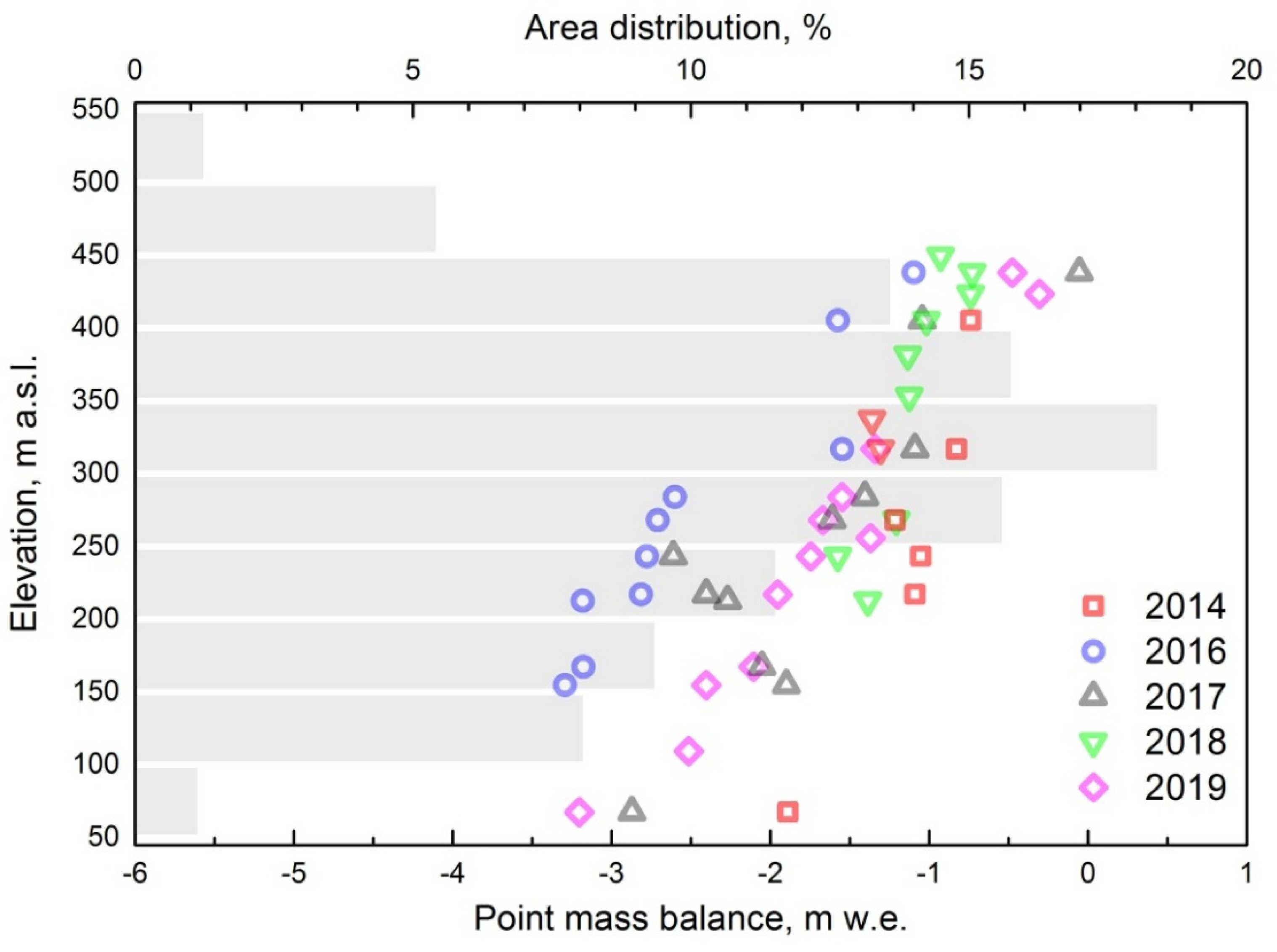
3.1. Surface Mass Balance Estimated by the Glaciological Method

Figure 5 shows the distribution of measured annual specific mass balance with altitude on Austre Grønfjordbreen in 2014, 2016–2019 years. The mass loss depended on elevation almost linearly and decreased with the altitude. The minimum and maximum point mass balances were −3.29 and −0.54 m w.e. in 2016 and 2017, respectively, with a mean value of −1.59 m w.e. The mean vertical gradient of annual mass balance varied from −0.8 m w.e. 100 m⁻¹ in 2016 to −0.4 m w.e. 100 m⁻¹ in 2014.

Measured values of mass balance are shown in

Table 4. Surface mass balance of Austre Grønfjordbreen.

Surface Mass Balance, m w.e.
Year	Net	Summer	Winter
2019	−1.51	−2.04	0.53
2018	−1.41
2017	−1.51
2016	−2.40
2015			0.77
2014	−1.10	−1.65	0.54
2013			0.62

. The annual mass balance was negative between 2014 and 2019, while the strongest loss was observed in 2016, caused by extremely high ablation due to high temperatures that stayed positive from May to November. The average summer temperature (Jun, July, August) in 2016 registered on Austre Grønfjordbreen was 5.9 °C, which is higher by 1 °C compared with the average summer temperatures from 2013 to 2019. The mass balance values including point measurements can be found in [11].

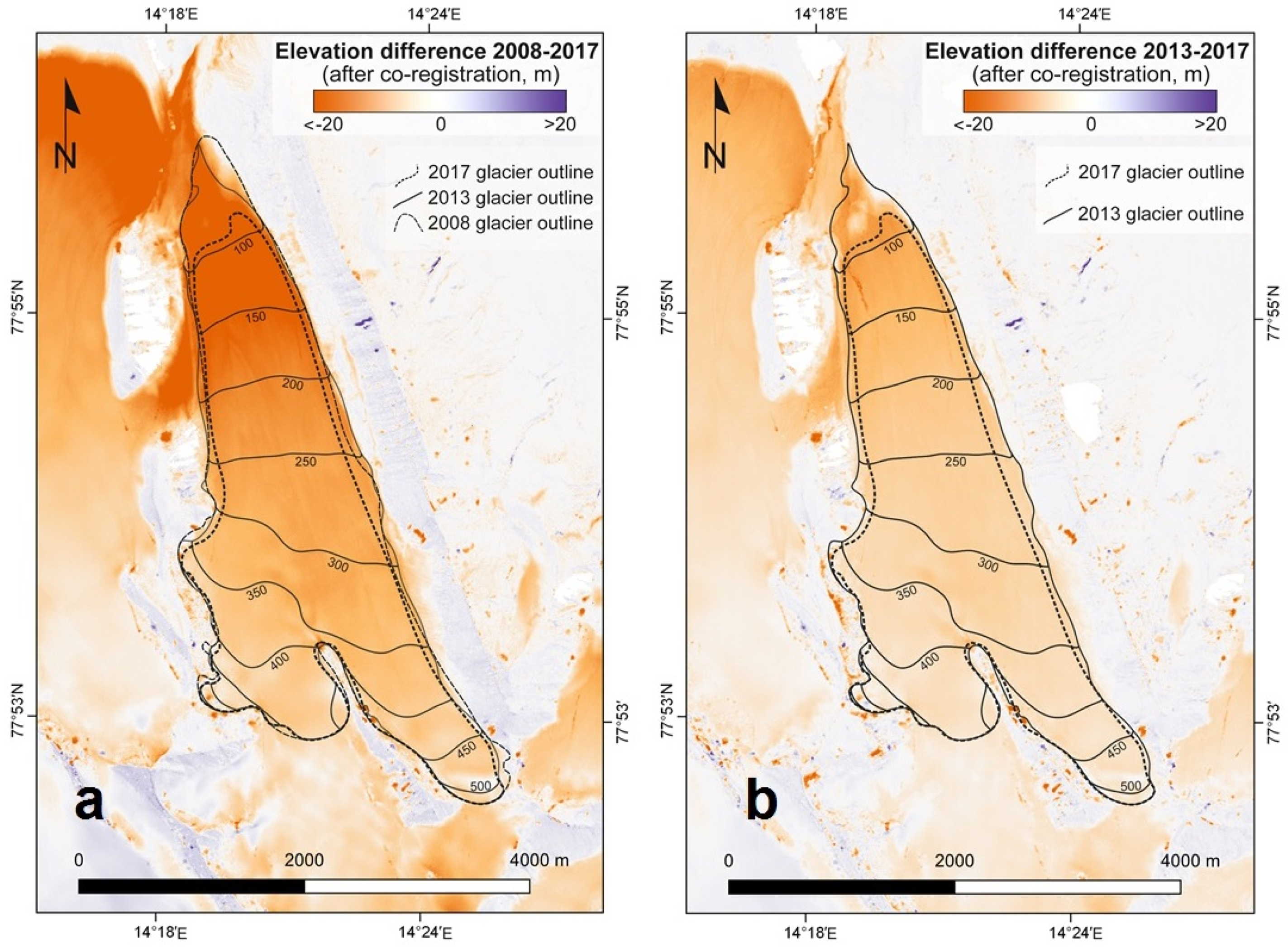
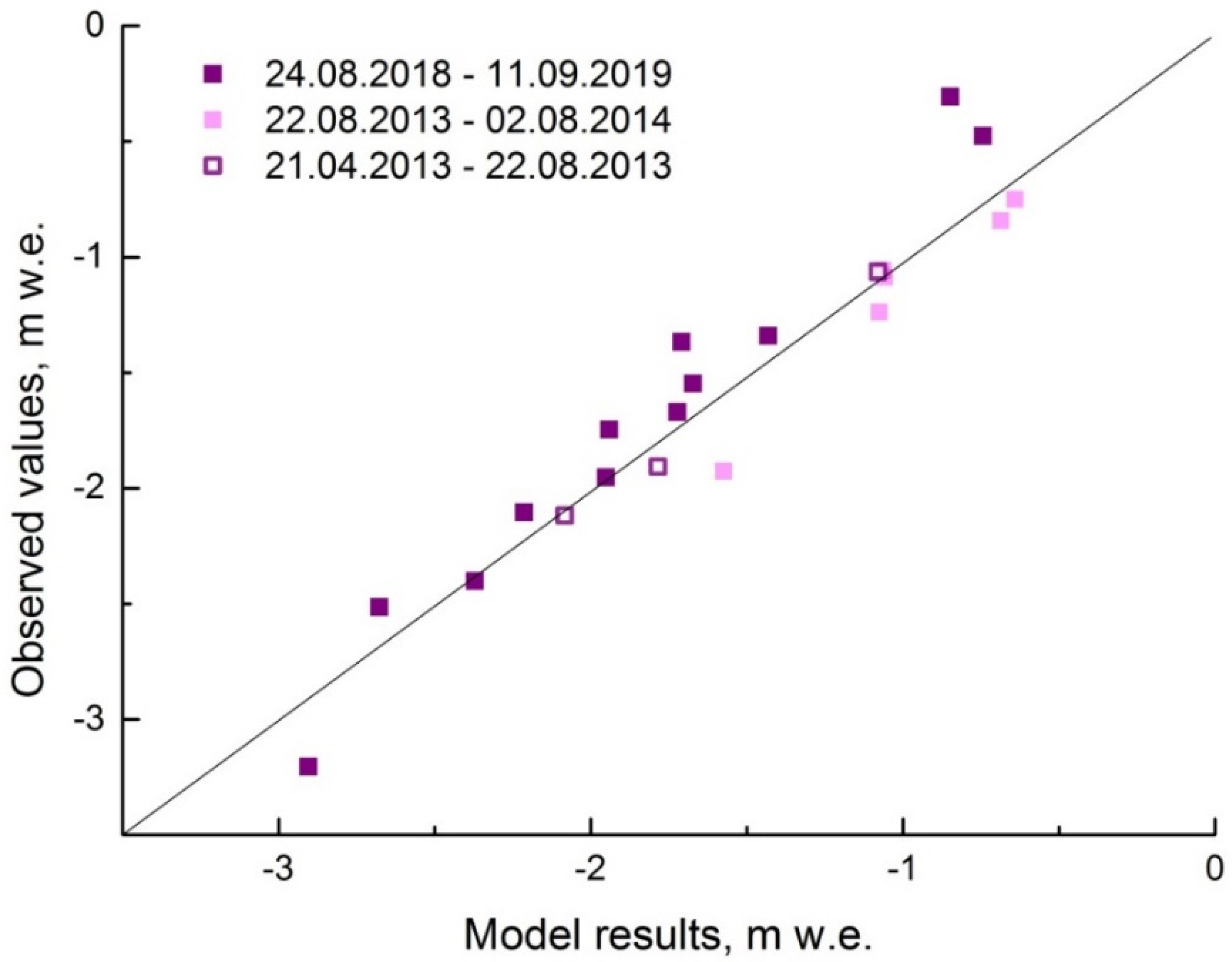
3.2. Geodetic Mass Balance

The geodetic mass balances of Austre Grønfjordbreen after DEM subtraction for 2013–2017 and 2008–2013 are as follows: 1) −1.45 m w.e.a^–1; and 2) −0.97 m w.e. a^–1. From 2008 to 2 August 2017, surface elevation decreased by −1.18 m w.e. a^–1. The distribution of the surface elevation differences for 2013–2017 and 2008–2017 is shown on Figure 6.

To make glaciological, geodetic and modelled mass balance comparable, we re-calculated the actual geodetic mass balance by adding the melting through the ending intervals of 2013 and 2017 ablation periods. These intervals are (1) from August 2, 2017 to 15 September 2017; and (2) from 17 August 2013 to 15 September 2013. The total melt in these two periods was estimated by the combination of stake observation data and DDF-approach. Thus, re-calculated geodetic mass balances for 2013–2017 and 2008–2013 were −1.54 m w.e. a^–1 and −1.15 m w.e. a^–1, correspondingly, which gives −1.34 m w.e. a^–1 for the entire period. Our results are comparable with the results of Aldegondabreen and Vøringbreen geodetic mass balances. Aldegondabreen (~ 6 km²; 100–450 m a.sl.) is located 9 km northwest of Austre Grønfjordbreen. The mass balance from 2015 to 2018 was −1.76 m w.e. a^–1 [33]. Vøringbreen (~0.75 km²; 180–400 m a.s.l.) is located 17 km northwest of Austre Grønfjordbreen, and its geodetic mass balance in 2013–2019 was −1.30 m w.e. a^–1 [34].

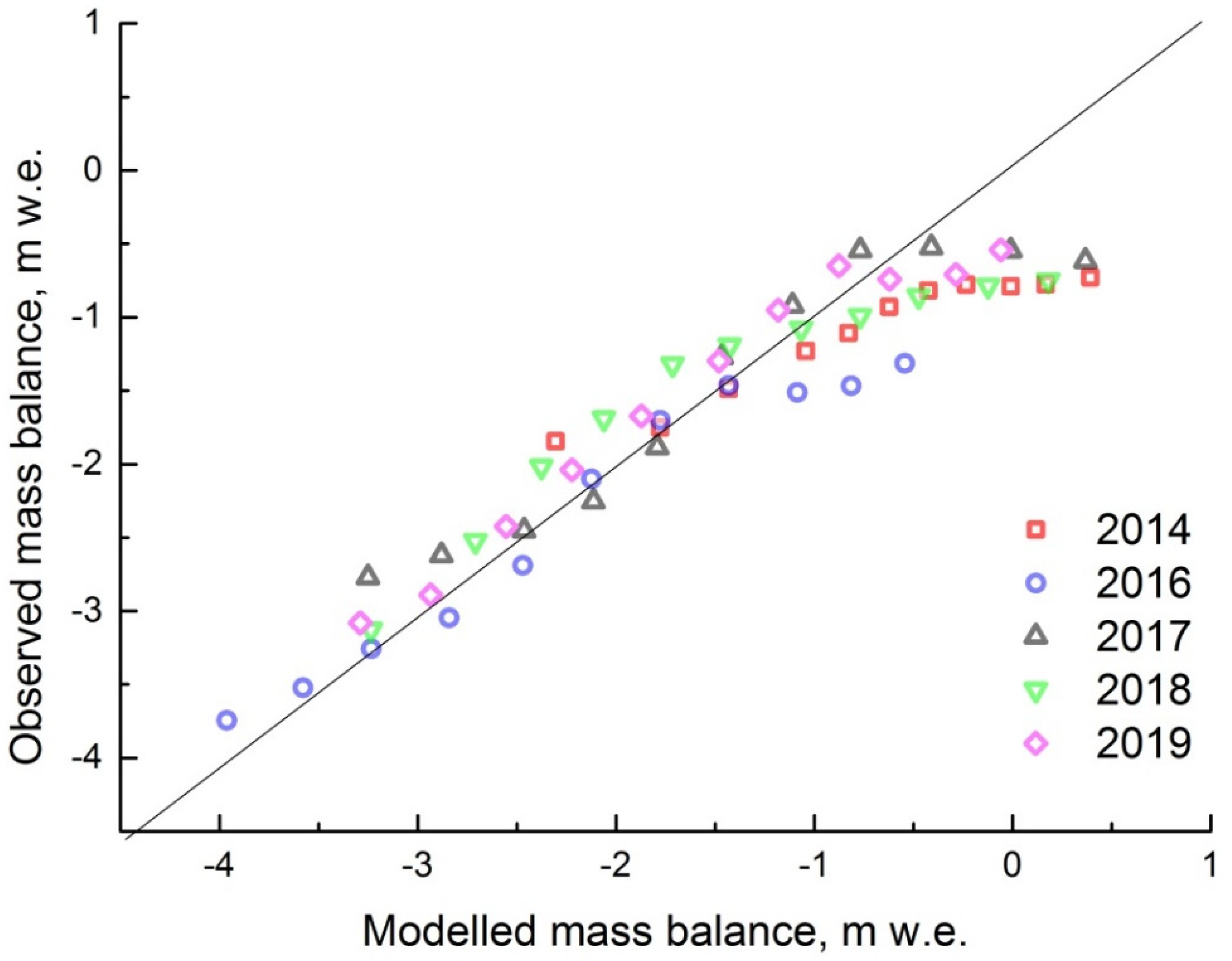
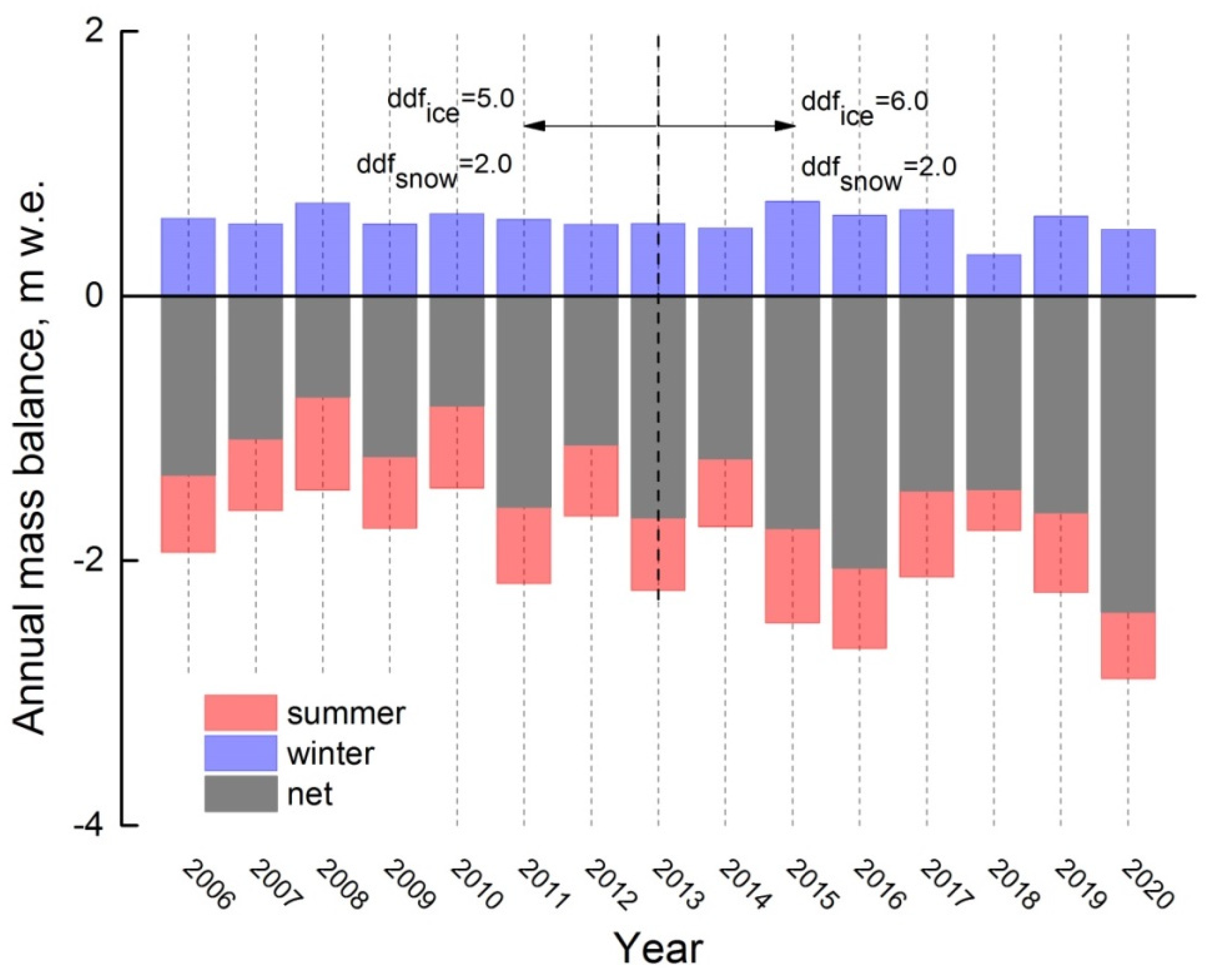
3.3. Mass-Balance Reconstruction by DDF Model

Modeled and measured annual mass balances for 5 years are compared in Figure 7. The temperature index modelling for 5 years was performed to match the exact dates of the field surveys (Table 1). The differences became larger as a function of elevation. Our results indicate that modeled and measured mass balances were in good agreement, with a correlation coefficient of R = 0.96 (p < 0.001) and root mean square error (RMSE) of 0.22 m w.e.

We also reconstructed the annual mass balance of Austre Grønfjordbreen for a longer period, namely from 2006 to 2020 (Figure 8). The model started on 16 September and ended on 15 April yearly from 2005 to 2019 for winter balance. Summer mass balance was simulated for the 16 April to 15 September period from 2006 to 2020. The reconstruction was done using unchanged DDFs and then separately for two periods, 2006–2013 and 2013–2020, with slightly different DDFs for ice.

Annual mass balances of Austre Grønfjordbreen were negative during the whole period and were the most negative in 2016 (−2.05 m w.e.) and 2020 (−2.39 m w.e.). It is worth noting that the highest temperature (21 °C) throughout the time series was recorded in July 2020. The least negative mass balance was found for 2008 (−0.76 m w.e) and 2010 (−0.83 m w.e.). The winter mass balance stayed within the interval from 0.36 to 0.71 m w.e.

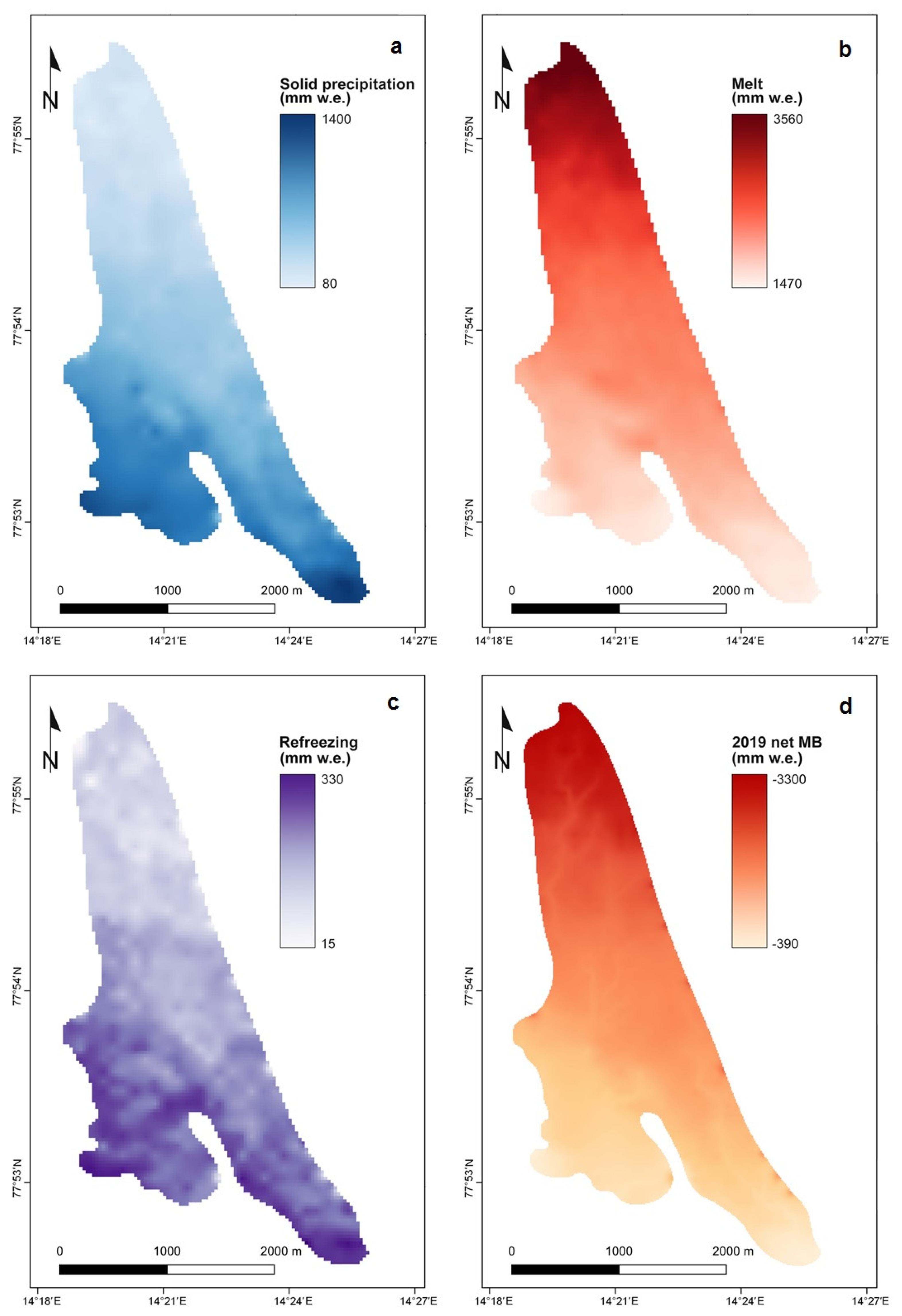
3.4. Spatially Distributed Mass Balance and its Components

The net mass balance and its components were modelled for 6 balance years using the A-Melt model. Model calibration was run over the observation period at spatial grid points where observational data existed (Figure 9). The modeled and measured mass balances were in the good agreement, with a correlation coefficient of R = 0.96 (p < 0.001) and RMSE = 0.13 mm w.e. The mass balance, solid precipitation, amount, melt and refreezing of Austre Grønfjordbreen are presented in

Table 5. The mass balance, solid precipitation amount, melt and refreezing of Austre Grønfjordbreen modelled for 4 balance years.

Balance Year	Net Mass Balance, m w.e.	Solid Precipitation, m w.e.	Melt, m w.e.	Refreezing, m w.e.
2019	−1.73	0.66	2.38	0.18
2015	−1.53	0.86	1.87	0.25
2014	−0.93	0.64	1.65	0.12
2013	−1.52	0.81	2.37	0.21
2012	−1.19	0.81	1.59	0.18
2011	−1.56	0.73	1.91	0.31

. Figure 10 shows spatial distributions of precipitation, melt, refreezing and climatic mass balance for one of the modelled balance years (2019). Austre Grønfjordbreen was shown to have less snow accumulation on the north side compared with its southern and south-western part of higher elevations, while overall melt rates were lowest in the south. The modelled mean net mass balance was negative (−1.41 m w.e) for 6 years, and there was no zone with positive values.

Averaged refreezing comprised 28% of the total accumulation from precipitation and amounted to 0.21 m w.e. a⁻¹. For comparison, a mean value for total refreezing of 0.30 m w.e. a⁻¹ was found on Holtedahlfonna and Kongsvegen by Van Pelt [35], and 0.24 m w.e. a^–1 for Kongsfjord basin was found in [36]. Refreezing varied spatially, with lower values in the north (0.15 m w. e. a⁻¹) than the south and south-west part (0.25 m w.e. a⁻¹). The firn layer was not considered because at the present state of the glacier, the firn thickness was negligibly thin.

4. Discussion

4.1. Differences in Mass Balance Assessment Approaches

The latest published work on Austre Grønfjordbreen mass balance [15] provides data measured by the glaciological method since 2004 and modeled using the empirical temperature approach. The latest published work on Austre Grønfjordbreen mass balance [15] provides data since 2004 as measured by the glaciological method and by modeling using the empirical temperature approach originally suggested by Krenke and Khodakov [37], in which the argument is the average summer air temperature with the parabolic dependence of the exponent of 3.25. (Figure 11).

Regarding the mass balance values obtained by the glaciological method in different studies, the discrepancy may be caused by several factors: the approach used to interpolate mass balance over the entire glacier area, the values of ice and snow density that is used for calculating accumulation and ablation into a water equivalent and averaging the winter mass balance value over several years, accounting for glacier area change. In [15], calculation of mass balance was carried out for four altitude zones. Surface ablation values were averaged in each altitude zone based on the stakes data. The density of ice was taken to be equal to 0.88 kg m⁻³. The snow accumulation was also averaged for each altitude zone, and four values were used for the entire period of mass balance record. All the values of net mass balance were calculated assuming that the balance year ends on 15 August. In this study we accounted for the glacier area decrease in each altitude zone, while in [15], it was considered constant. The glacier area recession was 15% in 2014–2020, and when such a change is not taken into account, a difference in mass balance calculation of 0.55 m w.e. a^–1 is obtained.

The model and reconstruction results were calibrated according to the stake measurements. Thus, the glaciological and modeled mass balances are in agreement for the calibration period. The reconstructed values of annual mass balance from 2014 to 2019 by day-degree method are 0.02 m w.e. a^–1 more negative than what was estimated using the glaciological methods. If using the DDFs = 6.0 and 2.0 mm °C⁻¹ d⁻¹ for ice and snow, correspondingly, the geodetic balance is less negative than reconstructed by the DDF model. The mean difference is 0.33 and 0.10 m w.e. a^–1 for 2008–2013 and 2013–2017, respectively. Therefore to make a better fit with geodetic results for 2008–2013, we calibrated DDFs again and used DDF_ice = 5.0 mm °C⁻¹ d⁻¹ and DDF_snow = 2.0 mm °C⁻¹ d⁻¹ (the mean difference is 0.01 m w.e. a^–1).

The mean mass balance differences between the geodetic and energy-balance approaches for the periods 2013–2017 and 2008–2013 are 0.22 m w.e. a^–1 and 0.16 m w.e. a^–1, respectively. We assume that a more accurate result can be reached using a more complex energy-balance model, compared to a DDF-approach using one set of parameters for the entire period of reconstruction. The DDF-approach requires the regular calibration of parameters and comparison with other methods, but it is useful as an approximation, and such meteorological parameters as temperature and precipitation are still more accessible for calculation.

4.2. Comparison with the Other Olaciers of the Archipelago

According to various authors cited in the IPCC report from 2006 to 2015, annual loss of Svalbard glaciers ranges from −250 ± 160 to −400 ± 230 kg m^–2 y^–1 [5]. The latest relevant review of the mass balance of Svalbard glaciers was carried out by Schuler et al. [10,38]. In particular, in this paper the comparison of several Svalbard-wide estimates of annual glacier mass balance using different methods is given. Summarizing the available data on the mass balance of Svalbard, authors in [10] estimated that Svalbard loses annually −7 ± 4 Gt (2000–2019) (the climatic mass balance) and −8 ± 6 Gt as the total mass balance.

Here we present the results of mass balance reconstruction of Austre Grønfjordbreen in comparison with 11 other glaciers of the archipelago. The most continuous mass balance series longer than 20 years exist for Austre Brøggerbreen, Midtre Lovénbreen, Kongsvegen Hansbreen and Waldemarbreen (

Table 6. The list of Svalbard glaciers with glaciological mass balance measurements considered in this study.

	Abbreviation	Elevation Range, m a.s.l.	Area, km2	Investigation Period	Mass Balance Data Reference
Austre Brøggerbreen	AB	50–600	6.1	1967–2018	[39]
Austre Grønfjordbreen	AG	70–550	6.2	2013–2019	this study
Austre Lovénbreen	AL	100–550	4.5	2008–2018	[11]
Etonbreen (Austfonna)	E	0–800	880.0	2004–2018	[39]
Hansbreen	H	0–510	56.7	1989–2018	[11]
Irenebreen	I	125–650	4.0	2002–2017	[11]
Kongsvegen	K	0–1050	101.9	1987–2018	[39]
Kronebreen/Holtedalsfonna	Kr	0–1361	370	2003–2018	[39]
Midtre Lovénbreen	ML	50–600	5.4	1968–2018	[39]
Nordenskiöldbreen 2	N	0–1200	206	2006–2018	[11]
Svenbreen	S	155–757	4.5	2010–2018	[40]
Waldemarbreen	W	100–570	2.4	1995–2017	[11]

).

The observed and reconstructed annual mass balance of Austre Grønfjordbreen from 2006 to 2020 is shown in Figure 12a, together with measured annual mass balances for 11 Svalbard glaciers for the same period. The cumulative curves for the entire monitoring period of all these glaciers are shown in Figure 12b.

The mass balance of all these glaciers was negative or close to zero for 2006–2018. In general, Austre Grønfjordbreen mass balance repeats the mass balance of other glaciers but is the most negative one with the mean value of reconstructed annual mass balance of −1.44 m w.e. a^–1. The western part of the archipelago is mostly influenced by the warm West Spitsbergen Current. The temperature depends on winter time sea ice; the southwest of Svalbard generally remains ice-free due to poleward heat transport through the current [41,42]. The series of mass balance observations of two glaciers (Irenebreen and Waldemarbreen) are the most negative besides for Austre Grønfjordbreen (–0.99 and −1.16 m w.e.a^–1, respectively). These glaciers are also situated on the west coast with a relatively small area. The glaciers of the same size class that are located slightly to the North (Austre Brøggerbreen, Austre Lovénbreen, Midtre Lovénbreen) have less negative mass balance (−0.60, −0.51 and −0.48 m w.e. a^–1, respectively). Less negative mass balances are found for larger glaciers, such as Kongsvegen, Etonbreen, Nordenskiöldbreen and Hansbreen (−0.09, −0.05, −0.07 and −0.31 m w.e. a^–1, respectively). Etonbreen is an outlet from the Austfonna ice cap, and its mass balance is close to zero. Schuler et al. [10] conclude that small glaciers experience more negative surface mass balances because they lose mass faster than large glaciers due to their hypsometric distributions of area with elevation.

All cumulative curves show the steady negative trend over the past 16 years. Over the period from 2006 to 2020, the cumulative mass balance of Austre Grønfjordbreen according to our modelling results was −21.62 m w.e. This is in agreement with the cumulative mass balances of glaciers in southern and central Spitsbergen rather than glaciers in the northwest of Svalbard concerning both small and large sized glaciers [10].

According to multi-temporal digital inventory of Svalbard glaciers by Nuth [6] and the original glacier inventory of Svalbard by Hagen [43], which followed the identification and parameter definitions outlined in the World Glacier Inventory [44], the largest relative area changes between the periods of these two inventories occurred in Nordenskiöld Land area. The results from [22] showed that the reduction of valley glaciers of Nordenskiöld Land is inversely proportional to their size. The elevation range is an important factor since it is directly related to the ablation. At higher altitudes, an increase of solid precipitation amount is usually observed if not taking into account orographic factors and precipitation distribution that can be complex. This increase can somewhat compensate the summer melting. However, the equilibrium line altitude (ELA) on Austre Grønfjordbreen is above the highest point of the glacier now.

The process of mass balance evolution varies in terms of the climatic regime and local meteorological conditions. The simulations made by Van Pelt et al. [42] for 2012–2016 include a long-term mean distribution of air temperature on Svalbard. The area nearby Austre Grønfjordbreen experienced relatively high temperature rates during the simulation period. At the given simulation based on the reanalysis the precipitation rate was minimal, and at the same time snow onset started relatively late and the disappearance was relatively early. The snow depth was minimal, but the rate of rainfall was relatively high [42], and these factors negatively affected glacier mass.

Available long-term mass balance observations on Svalbard show the impact of regional climatic aspects as well as the hypsometric differences. Austre Grønfjordbreen mass balance is the lowest among other observed glaciers due to a combination of factors: low elevation range, location on the western part of Central Spitsbergen and a small area with the absence of an accumulation zone.

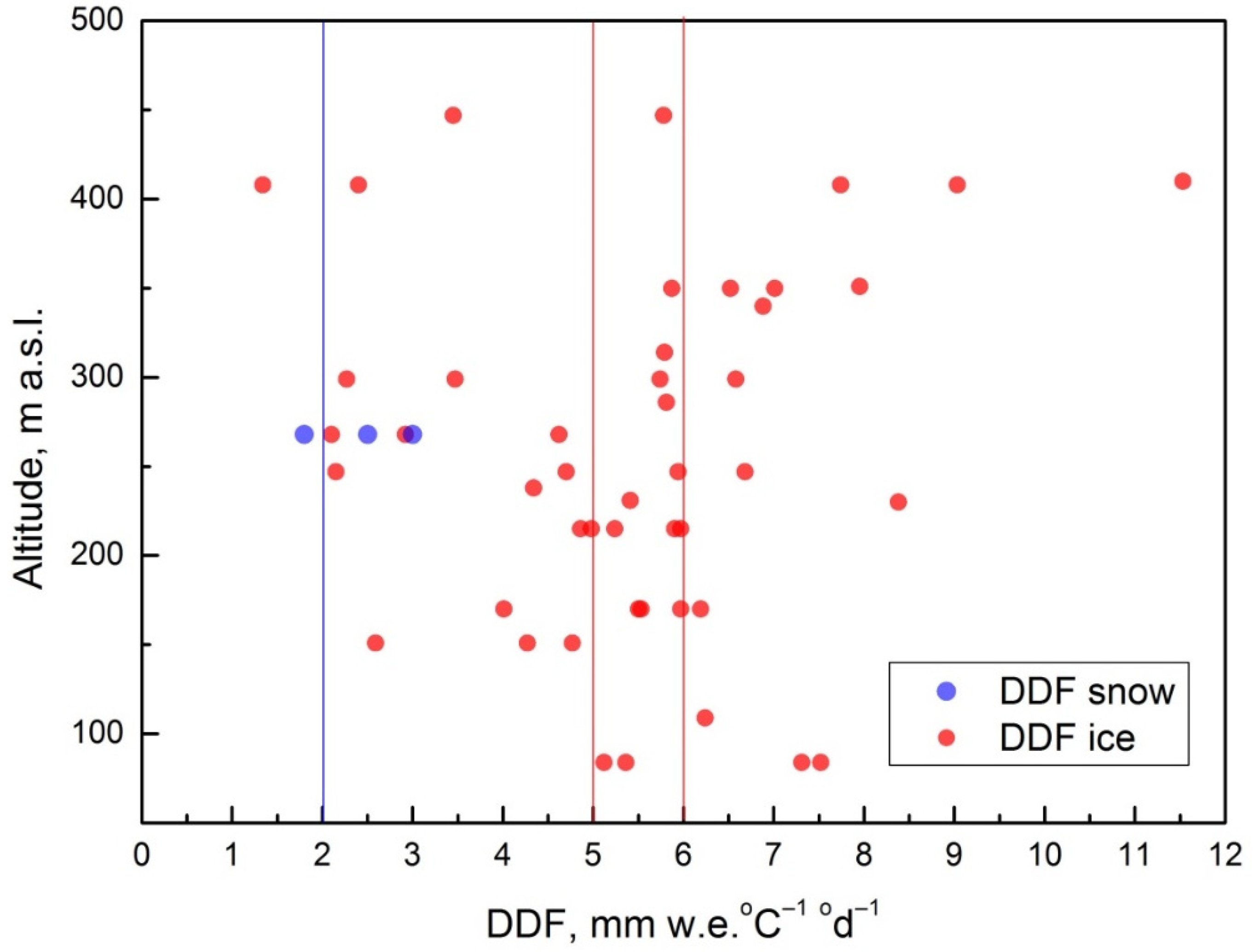
4.3. Degree-Day Factors Variations

Temperature and precipitation are not the only factors affecting the glacier mass balance, though the role of air temperature is explained by the fact that it is a universal characteristic of almost all components of the heat balance [37]. In fact, the overall mass change is determined mainly by the energy balance at the glacier surface. Thus, as a simplification, DDFs physically parameterize energy balance components that have an influence on melting. Individual energy components that provide energy for melting vary in space and time, and thus DDF meanings are different for individual glaciers [29], and therefore the degree-day approach does not accurately represent the spatial variability of melt over the entire glacier surface. Reported values of degree-day factors of glaciers and snow-covered basins can be found in [28,29]. At the same time, the DDFs used at a century timescale and that remained stable until the mid of 1970s have decreased by 7% per decade [45]; therefore, DDFs must be used with caution and only for reconstructing changes over short periods of time.

For Svalbard, a variability of degree-day factors for snow and ice has been overviewed by Möller and Kohler [12]. The degree-day factors for snow are in the range of 3 −24 mm C^–1 d^–1, and 9–13.8 mm C^–1 d^–1 for ice [12]. On Kongsvegen, the 21 year stake record results in a DDF of 3.0 mm C⁻¹ d⁻¹ for snow and 3.5 mm C⁻¹ d⁻¹ for ice [46]. On Kronebreen, the DDF for snow is 3.1 mm C⁻¹ d⁻¹ and 4.7 mm C⁻¹ a⁻¹ for ice [46]. Hence, our calibration results of 5.0 and 6.0 mm C⁻¹ d⁻¹ for ice and 2.0 mm C^–1 d^–1 for snow surfaces are reasonable and are in good accordance with the previously reported DDFs for Svalbard.

4.4. Sensitivity Tests

Assessment of glacier mass-balance sensitivity to climate change enables interpretation of the glacier–climate interaction. Surface mass balance sensitivity to air temperature, solar radiation, precipitation and topographical variables is necessary to calibrate/validate the numerical models used to simulate the evolution of glaciers [47].

The mass-balance sensitivity of Austre Grønfjordbreen to climatic fluctuation was assessed over the period 2014–2019. The average annual mass balance was recalculated by re-running the degree-day model with the same parameters, but assuming a 1 °C increase in temperature or a 10% change in precipitation throughout the balance year. Mass-balance sensitivity to air temperature (dMB/dT) and precipitation (dMB/dP) was calculated as the difference between the modelled values.

The calculated mass-balance sensitivity to air temperature is −1.04 m w.e °C ⁻¹, which corresponds to the highest sensitivity on Svalbard among the assessed by temperature-index model.

Sensitivity values of net mass balance to temperature change (1 °C increase) assessed by the degree-day approach for Austre Brøggerbreen, Midtre Lovénbreen, Kongsvegen and Hansbreen are −0.49, −0.48, −0.69 and −0.49 (m w.e. a^–1), respectively [48].

The same sensitivity test was also conducted for precipitation. Calculated mass balance sensitivity to precipitation for Austre Grønfjordbreen is 0.10 m w.e. for a 10% change. For both Midtre Lovénbreen and Kongsvegen, the sensitivity for 10% change in precipitation is 0.05 (m w.e. a^–1), and a 31% increase of snow precipitation is needed to compensate for the net mass loss induced by an air temperature increase of +1°C [48].

In a number of papers on Svalbard glaciers, the mass balance sensitivity to changes in air temperature and the amount of precipitation is estimated using energy balance models [35,36,49,50]. For example Van Pelt et al. [49] assessed the sensitivity for Nordenskiöldbreen as 0.10 m w.e. for a 10% change in precipitation and −0.36 m w.e for a 1 °C increase in temperature. A 1 °C temperature change can be offset by a 32% change in precipitation of a similar sign in cases of seasonally uniform perturbations [49]. For Midtre Lovénbreen, Kongsvegen and Holtedahfonna, the mass balance will change by 0.13; 0.12; 0.13 (m w.e. a^–1), respectively, in case of 10% precipitation change and the rise of 1 °C will lead to mass balance decrease of −0.83, −0.69 and −0.55 (m w.e. a^–1), respectively [36].

In order to assess the precipitation amount that is needed to offset the mass loss due to a 1 °C rise, we adjusted the model several times until the increased melting could be covered by the adjusted precipitation, while the other model parameters were kept unchanged. The result showed that a two-fold increase in precipitation could compensate the increased mass loss due to air temperature rise.

5. Conclusions

We estimated the surface mass balance of Austre Grønfjordbreen using the glaciological method for 5 years during the period 2014–2020. The average annual value for this period is −1.59 m w.e. After a negative 2016 balance year (−2.40 m w.e.), the accumulation area of the glacier disappeared completely.

The geodetic mass balance from 2008 to 2017 is also negative but is within less negative intervals than observed and modeled by two methods. For the period of 2013–2017, the geodetic mass balance is −1.54 m w.e. a^–1, including the melting that occurred during the period of the end of the balance year. For 2008–2013 the mass balance is −1.15 m w.e. a^–1.

For the period 2006–2020, the annual, summer and winter mass balances were reconstructed by the temperature-index model and simple accumulation model. We found that Austre Grønfjordbreen lost −21.62 m w.e. over the period of 15 balance years.

The calculated mass-balance sensitivity to air temperature is −1.04 m w.e. °C⁻¹ and to precipitation is 0.10 m w.e. for a 10% increase. The sensitivity to temperature change is the highest among the reported for Svalbard. A two-fold increase in precipitation could offset the increased mass loss due to a 1 °C air temperature rise. The summer air temperature was found to be a stronger driver of mass balance than the winter precipitation.

We used a surface energy-balance model, A-Melt, to simulate the spatial distribution of mass balance and its components. The model is forced with meteorological data from AWS Barentsburg, Adventdalen radiation data and available field snow measurements on a 100 m × 100 m grid. Calibration is performed by adjusting the temperature lapse rate and precipitation gradient to match the measured mass balance data. The net mass balance is estimated to an average of −1.43 m w.e. a⁻¹ over the simulation period.

Comparing the mass balance of Austre Grønfjordbreen with the mass balance of other glaciers that are monitored on Svalbard, the glacier experiences the highest rate of mass loss. Among the reasons for this difference is the location in the part of the archipelago that supposedly has one of the highest rates of the mass loss, its low altitude interval, relatively small area, as well as the total absence of an accumulation area.

This study provides the information for mass balance estimations in the western part of Nordenskiöld Land and is a basis for projecting future glacier evolution in this area.

References

1. Zemp, M.; Huss, M.; Thibert, E.; Eckert, N.; McNabb, R.; Huber, J.; Barandun, M.; Machguth, H.; Nussbaumer, S.U.; Gärtner-Roer, I. Global glacier mass changes and their contributions to sea-level rise from 1961 to 2016. Nature 2019, 568, 382–386. [Google Scholar] [CrossRef]
2. Dyurgerov, M.B.; Meier, M.F. Twentieth century climate change: Evidence from small glaciers. Proc. Natl. Acad. Sci. USA 2000, 97, 1406–1411. [Google Scholar] [CrossRef] [Green Version]
3. Kaser, G.; Cogley, J.G.; Dyurgerov, M.B.; Meier, M.F.; Ohmura, A. Mass balance of glaciers and ice caps: Consensus estimates for 1961–2004. Geophys. Res. Lett. 2006, 33, L19501. [Google Scholar] [CrossRef] [Green Version]
4. Hock, R.; Bliss, A.; Marzeion, B.; Giesen, R.H.; Hirabayashi, Y.; HUSS, M.; Radic, V.; Slangen, A.B.A. GlacierMIP–A model intercomparison of global-scale glacier mass-balance models and projections. J. Glaciol. 2019, 65, 453–467. [Google Scholar] [CrossRef] [Green Version]
5. IPCC Special Report: The Ocean and Cryosphere in a Changing Climate (final draft). IPCC Summ. Policymalers 2019. Available online: https://www.ipcc.ch/report/srocc/ (accessed on 12 December 2019).
6. Nuth, C.; Kohler, J.; König, M.; von Deschwanden, A.; Hagen, J.O.; Kääb, A.; Moholdt, G.; Pettersson, R. Decadal changes from a multi-temporal glacier inventory of Svalbard. Cryosphere 2013, 7, 1603–1621. [Google Scholar] [CrossRef] [Green Version]
7. Martín-Español, A.; Navarro, F.J.; Otero, J.; Lapazaran, J.J.; Błaszczyk, M. Estimate of the total volume of Svalbard glaciers, and their potential contribution to sea-level rise, using new regionally based scaling relationships. J. Glaciol. 2015, 61, 29–41. [Google Scholar] [CrossRef] [Green Version]
8. Jania, J.; Hagen, J.O. Mass Balance of Arctic Glaciers; International Arctic Science Committee: Katowice, Poland, 1996; ISBN 8390564343. [Google Scholar]
9. Hagen, J.O.; Melvold, K.; Pinglot, F.; Dowdeswell, J.A. On the net mass balance of the glaciers and ice caps in Svalbard, Norwegian Arctic. Arct. Antarct. Alp. Res. 2003, 35, 264–270. [Google Scholar] [CrossRef] [Green Version]
10. Schuler, T.V.; Kohler, J.; Elagina, N.; Hagen, J.O.M.; Hodson, A.J.; Jania, J.A.; Kääb, A.M.; Luks, B.; Małecki, J.; Moholdt, G. Reconciling Svalbard Glacier Mass Balance. Front. Earth Sci. 2020, 8, 1–31. [Google Scholar] [CrossRef]
11. WGMS (World Glacier Monitoring Service) Fluctuations of Glaciers Database. Available online: http://dx.doi.org/10.5904/wgms-fog-2020-08 (accessed on 1 March 2020).
12. Möller, M.; Kohler, J. Differing Climatic Mass Balance Evolution Across Svalbard Glacier Regions Over 1900–2010. Front. Earth Sci. 2018, 6, 1–20. [Google Scholar] [CrossRef] [Green Version]
13. Troitsky, L.S. On the mass balance of different types of glaciers in Spitsbergen. Mater. Glyatsiologicheskikh Issled. Data Glaciol. Stud. 1988, 1, 117–121. [Google Scholar]
14. Mavlyudov, B.; Savatyugin, L.; Solovyanova, I. The reaction of the glaciers of the Nordenskiold Land (Spitsbergen) to climate change. Probl. Arct. Antarct. 2012, 1, 67–77. [Google Scholar]
15. Chernov, R.A.; Kudikov, A.V.; Vshivtseva, T.V.; Osokin, N.I. Estimation of the surface ablation and mass balance of Austre Grønfjordbreen (Spitsbergen). Ice Snow 2019, 59, 59–66. [Google Scholar] [CrossRef]
16. Sosnovsky, A.V.; Macheret, Y.Y.; Glazovsky, A.F.; Lavrentiev, I.I. Influence of snow cover on the thermal regime of a polythermal glacier in Western Spitsbergen. Ice Snow 2015, 131, 27. [Google Scholar] [CrossRef] [Green Version]
17. Lavrentiev, I.I.; Kutuzov, S.S.; Glazovsky, A.F.; Macheret, Y.Y.; Osokin, N.I.; Sosnovsky, A.V.; Chernov, R.A.; Cherniakov, G.A. Snow thickness on Austre Grønfjordbreen, Svalbard, from radar measurements and standard snow surveys. Ice Snow 2018, 58, 5–20. [Google Scholar] [CrossRef]
18. Rets, E.; Kireeva, M. Hazardous hydrological processes in mountainous areas under the impact of recent climate change: Case study of Terek River basin. IAHS-AISH Publ. 2010, 340, 126–134. [Google Scholar]
19. Belozerov, E.; Rets, E.; Petrakov, D.; Popovnin, V. Modelling glaciers’ melting in Central Caucasus (the Djankuat and Bashkara Glacier case study). E3S Web Conf. 2020, 163, 01002. [Google Scholar] [CrossRef]
20. Rets, E.; Barandun, M.; Belozerov, E.; Petrakov, D.; Shpuntova, A. Mass-balance modelling of Ak-Shyirak massif Glaciers, Inner Tian Shan.; EGU General Assembly: Vienna, Austria, 2017; p. 10327. [Google Scholar]
21. Rets, E.P.; Petrakov, D.A.; Belozerov, E.V.; Shpuntova, A.M. Sary-Tor glaier mass balance modelling (the Ak-Shiyrak massif, inner Tien Shan). Earth’s Cryoshpere 2021, in press. [Google Scholar]
22. Chernov, R.A.; Muraviev, A.Y. Contemporary changes in the area of glaciers in the western part of the Nordenskjold Land (Svalbard). Led i Sneg 2018, 462–472. [Google Scholar] [CrossRef]
23. Norwegian Polar Institute (npolar.no) TopoSvalbard Map Service. Available online: https://toposvalbard.npolar.no/ (accessed on 18 November 2020).
24. König, M.; Kohler, J.; Nuth, C. Glacier Area Outlines - Svalbard [Data set]. Norwegian Polar Institute. Available online: https://data.npolar.no/dataset/89f430f8-862f-11e2-8036-005056ad0004 (accessed on 25 January 2020).
25. Nuth, C.; Kääb, A. Co-registration and bias corrections of satellite elevation data sets for quantifying glacier thickness change. Cryosphere 2011, 5, 271–290. [Google Scholar] [CrossRef] [Green Version]
26. ArcticDEM. Available online: https://www.pgc.umn.edu/data/arcticdem (accessed on 17 October 2020).
27. Norwegian Polar Institute. Terrengmodell Svalbard (S0 Terrengmodell) [Data Set]. Available online: https://doi.org/10.21334/npolar.2014.dce53a47 (accessed on 17 October 2020).
28. Braithwaite, R.J.; Zhang, Y. Sensitivity of mass balance of five Swiss glaciers to temperature changes assessed by tuning a degree-day model. J. Glaciol. 2000, 46, 7–14. [Google Scholar] [CrossRef] [Green Version]
29. Hock, R. Temperature index melt modelling in mountain areas. J. Hydrol. 2003, 282, 104–115. [Google Scholar] [CrossRef]
30. Kuzmin, P.P. The Process of Snow Melting; Gidrometizdat: Leningrad, Russia, 1961. [Google Scholar]
31. The University Centre in Svalbard UNIS Weather stations and CTD stations. Available online: https://www.unis.no/resources/weather-stations/ (accessed on 3 March 2020).
32. Institute of Applied Astronomy of the Russian Academy of Sciences Online Ephemeris Service. Available online: http://iaaras.ru/dept/ephemeris/online/ (accessed on 4 March 2020).
33. Terekhov, A.V.; Tarasov, G.V.; Sidorova, O.R.; Demidov, V.E.; Anisimov, M.A.; Verkulich, S.R. Estimation of mass balance of Aldegondabreen (Spitsbergen) in 2015–2018 based on ArcticDEM, geodetic and glaciological measurements. Ice Snow 2020, 192–200. [Google Scholar] [CrossRef]
34. Terekhov, A.V.; Demidov, V.E.; Kazakov, E.E.; Anisimov, M.A.; Verkulich, S.R. Geodetic mass balance of Vöring Glacier, Western Spitsbergen, in 2013–2019. Kriosf. Zemli 2020, 14, 55–63. [Google Scholar] [CrossRef]
35. Van Pelt, W.; Kohler, J. Modelling the long-term mass balance and firn evolution of glaciers around Kongsfjorden, Svalbard. J. Glaciol. 2015, 61, 731–744. [Google Scholar] [CrossRef] [Green Version]
36. Pramanik, A.; Van Pelt, W.; Kohler, J.; Schuler, T.V. Simulating climatic mass balance, seasonal snow development and associated freshwater runoff in the Kongsfjord basin, Svalbard (1980–2016). J. Glaciol. 2018, 64, 943–956. [Google Scholar] [CrossRef] [Green Version]
37. Krenke, A.M.; Khodakov, V.G. Connection of the surface melting glaciers and air temperature. Mater. Glyatsiologicheskikh Issled. Data Glaciol. Stud. 1966, 1, 153–164. [Google Scholar]
38. Schuler, T.V.; Glazovsky, A.; Hagen, J.O.; Hodson, A.; Jania, J.; Kohler, J.; Malecki, J.; Moholdt, G.; Pohjola, V.; Van Pelt, W.; et al. New data, new techniques and new challenges for updating the state of Svalbard glaciers (SvalGlac). 2019, 4, 1–22. [Google Scholar]
39. Kohler, J. Mass balance for glaciers near Ny-Ålesund [Data set]. Norwegian Polar Institute. Available online: https://doi.org/10.21334/npolar.2013.ad6c4c5a (accessed on 1 March 2020).
40. Malecki, J. Annual mass balance of Svenbreen, Central Spitsbergen, Svalbard [Data set]. Adam Mickiewicz University. Available online: https://doi.org/10.21334/npolar.2020.b3bb4ee2 (accessed on 1 March 2020).
41. Walczowski, W.; Piechura, J. Influence of the West Spitsbergen Current on the local climate. Int. J. Climatol. 2011, 31, 1088–1093. [Google Scholar] [CrossRef]
42. Van Pelt, W.J.J.; Kohler, J.; Liston, G.E.; Hagen, J.O.; Luks, B.; Reijmer, C.H.; Pohjola, V.A. Multidecadal climate and seasonal snow conditions in Svalbard. J. Geophys. Res. Earth Surf. 2016, 121, 2100–2117. [Google Scholar] [CrossRef]
43. Hagen, J.O.; Liestøl, O.; Roland, E.; Jørgensen, T. Glacier atlas of Svalbard and Jan Mayen. Norwegian Polar Institue: Oslo, Norway, 1993; ISBN 8276660665. [Google Scholar]
44. Haeberli, W.; Bösch, H.; Scherler, K.; Østrem, G.; Wallén, C.C. WGMS (1989): World glacier inventory – Status 1988; World Glacier Monitoring Service: Zurich, Switzerland, 1989. [Google Scholar]
45. Huss, M.; Bauder, A.; Funk, M. Homogenization of long-term mass-balance time series. Ann. Glaciol. 2009, 50, 198–206. [Google Scholar] [CrossRef] [Green Version]
46. Nuth, C.; Schuler, T.V.; Kohler, J.; Altena, B.; Hagen, J.O. Estimating the long-term calving flux of Kronebreen, Svalbard, from geodetic elevation changes and mass-balance modeling. J. Glaciol. 2012, 58, 119–133. [Google Scholar] [CrossRef] [Green Version]
47. Reveillet, M.; Vincent, C.; Six, D.; Rabatel, A. Which empirical model is best suited to simulate glacier mass balances? J. Glaciol. 2017, 63, 39–54. [Google Scholar] [CrossRef] [Green Version]
48. Xu, M.; Yan, M.; Kang, J.; Ren, J. Comparative studies of glacier mass balance and their climatic implications in Svalbard, Northern Scandinavia, and Southern Norway. Environ. Earth Sci. 2012, 67, 1407–1414. [Google Scholar] [CrossRef]
49. Van Pelt, W.J.J.; Oerlemans, J.; Reijmer, C.H.; Pohjola, V.A.; Pettersson, R.; van Angelen, J.H. Simulating melt, runoff and refreezing on Nordenskiöldbreen, Svalbard, using a coupled snow and energy balance model. Cryosphere 2012, 6, 641–659. [Google Scholar] [CrossRef] [Green Version]
50. Østby, T.I.; Schuler, T.V.; Hagen, J.O.; Hock, R.; Kohler, J.; Reijmer, C.H. Diagnosing the decline in climatic mass balance of glaciers in Svalbard over 1957–2014. Cryosphere 2017, 11, 191–215. [Google Scholar] [CrossRef] [Green Version]
Figure 1. (a) Glaciers with ongoing mass balance measurements on Svalbard (Table 6). The map is provided by © Norwegian Polar Institute (npolar.no) [23]; (b) observation network on Austre Grønfjordbreen. The background is a Landsat image (14 September 2017). The glacier outline of 1936 is delivered by the CryoClim service with the © Norwegian Polar Institute (npolar.no) [24].
Geosciences 11 00078 g001
Figure 2. (a) Mean monthly temperature and precipitation values from 2005 to 2019 recorded on AWS Barentsburg; (b) Mean temperature values of the warmest months from 2005 to 2019.
Geosciences 11 00078 g002
Figure 3. Elevation difference distribution before and after co-registration. (a) Elevation difference 2013–2017. The shift between two DEMs was considered as negligible. Then co-registration procedure was not applied; (b) dH distribution 2013–2017; (c) elevation difference 2008–2017. Sinusoidal shift approximation line shows the necessity of co-registration application; (d) dH distribution 2008–2017.
Geosciences 11 00078 g003
Figure 4. The variety of observed DDFs for snow and ice measured from the stakes. Blue and red lines show the DDFs for snow and ice that were used after the model was calibrated.
Geosciences 11 00078 g004
Figure 5. Single point mass balance values at the stakes location for 5 years and area distribution of Austre Grønfjordbreen in 2019.
Geosciences 11 00078 g005
Figure 6. The map of the dH distribution of Austre Grønfjordbreen for: (a) 2008–2017; (b) 2013–2017.
Geosciences 11 00078 g006
Figure 7. Comparison of modeled and observed annual mass balance for 5 years.
Geosciences 11 00078 g007
Figure 8. Reconstructed summer, winter balance and net balance of Austre Grønfjordbreen from 2006 to 2020.
Geosciences 11 00078 g008
Figure 9. Relation between observed stake measurements and modelled melt after the calibration of A-Melt model.
Geosciences 11 00078 g009
Figure 10. Spatially distributed mass balance components: (a) solid precipitation; (b) melt; (c) refreezing and (d) net mass balance averaged for 2019 balance year.
Geosciences 11 00078 g010
Figure 11. Mass balance estimates by different methods from this study and Chernov et al. [15].
Geosciences 11 00078 g011
Figure 12. (a) The net balance throughout the monitoring periods for 12 glaciers including modelled annual mass balance of Austre Grønfjordbreen; (b) the cumulative mass balance throughout the monitoring periods for 12 glaciers modified from Schuler et al. [10,38].
Geosciences 11 00078 g012